Abstract

In this presentation, we review the general features of integrand-reduction techniques, with a particular focus on their generalization beyond one loop. We start with a brief discussion of the one-loop scenario, a case in which integrand-reduction algorithms are well established and played over the past decade an important role in the development of automated tools for the theoretical evaluation of physical observables. The generalization of integrand-reduction techniques to all loops has been the subject of several efforts in the recent past, thus providing a better understanding of the universal properties of scattering amplitudes. The ultimate goal of these studies is the development of efficient alternative computational techniques for the evaluation of Feynman integrals beyond one loop.

1 Introduction

Integrand-reduction techniques evolved enormously over the past decade. Since the one-loop 4-dimensional integrand reduction, also known as OPP method, introduced a new way of approaching the problem of the reduction of one-loop Feynman integrals [1], integrand reduction grew into a more general and variegated framework. Such advancements are due to several different authors and groups. A number of excellent review papers have been written on the subject and we refer the interested reader to them for more details and a more inclusive picture of the field [2].

In this talk, I will review some of the important steps along this evolution process, trying to underline the features that render integrand reduction a promising approach to study multi-loop scattering amplitudes. Most examples are taken from collaborative work in which I have been directly involved. They represent only a small part of the rich literature on the subject .

The presentation is organized as follows. I will start by defining the integrand-level approach to the reduction of scattering amplitudes, as compared with their integral-level description; I will then describe of the generalization of the integrand-level approach to higher loops, which was conveniently described using the language of multivariate polynomial division in algebraic geometry, and allowed to prove to a powerful theorem that shows the feasibility of such construction; After a brief excursus about the evolution of the numerical algorithms for one-loop calculations based on integrand reduction, I will give a short description of the GoSam framework and comment on the ongoing efforts towards its application beyond one loop.

2 Integrand level vs Integral level

In order to introduce the notation and better define what we call the integrand-level reduction, let’s consider a two-loop Feynman integral with n denominators:

$${\cal I}=\int dq\int dk\ {\cal A}({q,k})=\int dq\int dk\ {{\cal N}({q,k})\over D_{1}D_{2}\ldots D_{n}}\,,$$ (1)

where $q$ and $k$ are the integration momenta. For the sake of this discussion, we don’t need to specify at this stage whether such momenta are purely four-dimensional or regularized in $d=4-2\epsilon$ dimensions. The choice will become relevant later on when we will describe specific reduction algorithms.

The integral-level approach leads to a description of ${\cal I}$ in terms of Master Integrals ${\cal I}_{i}$. The integral in Eq. (1), can be rewritten as

$${\cal I}=\int dq\int dk\ {{\cal N}({q,k})\over D_{1}D_{2}\ldots D_{n}}=c_{0}\ {{\cal I}_{0}}+c_{1}\ {{\cal I}_{1}}+\ldots+C_{k}\ {{\cal I}_{k}}$$ (2)

for example by using tensorial reduction, exploring physical properties such as Lorentz invariance, or projecting the numerator to define convenient form factors. The initial integral is rewritten as a linear combination of Master Integrals (MI) which are in principle general and easier to compute than the original integral at hands. If we are able to compute all MIs, the knowledge of the sets of coefficients which are in front of them is sufficient to solve the problem.

As an alternative path, we can manipulate the integrand ${\cal A}({q,k})$ of Eq. (1) and cast it to a more convenient form before tackling the integration. Such approach leads to the integrand-level reduction. The advantage of this approach is that integrands are much simpler to handle than integrals, since they are all rational functions, namely ratios of polynomials written in terms of integration variables and physical momenta and masses of the various particles involved in the scattering process. Moreover, the structure of the poles of ${\cal A}({q,k})$, which play such an important role in field theory, is explicit in the integrand, as the set of zeros of the denominators. The question is how to use this knowledge to manipulate ${\cal N}(q,k)$, and therefore ${\cal A}(q,k)$, to obtain a simpler decomposition after we put it back under the integral sign.

Of course the two approaches are deeply interconnected. Taking a look at the one-loop scenario provides insights on their relation. In fact, at one loop, a general integral-level decomposition is well-known [4]:

$$\int dq\,\frac{{\mathcal{N}(q)}}{D_{1}D_{2}\ldots D_{n}} = \sum_{\{i\}}{d_{i}}\int\frac{dq}{D_{i_{1}}D_{i_{2}}D_{i_{3}}D_{i_{4}}}+\sum_{\{i\}}{c_{i}}\int\frac{dq}{D_{i_{1}}D_{i_{2}}D_{i_{3}}}$$ (3)

$$+ \sum_{\{i\}}{b_{i}}\int\frac{dq}{D_{i_{1}}D_{i_{2}}}+\sum_{i}{a_{i}}\int\frac{dq}{D_{i}}+{{\rm R}}\,.$$

According to the decomposition in Eq. (3), any $n$-point Feynman integral, independently from the number of legs, can be written as a linear combination of 4-point, 3-point, 2-point, and 1-point scalar integrals, which therefore represent a complete set of MI at one loop, plus an additional “constant” term ${{\rm R}}$ know as the rational part. Since all scalar integrals are known and available in public codes [5], the main problem in the evaluation of Feynman integrals lies in the evaluation of all the coefficients which multiply each MI.

Eq. (3) can be used as a map to find the corresponding integrand-level counterpart. If, for simplicity of notation, we consider purely four-dimensional integration momenta, where the rational part is absent, the integrand-level decomposition will have the form [1]

$${\mathcal{N}(q)} = \sum_{\{i\}}\Big{[}{d_{i}}+{\tilde{d_{i}}(q)}\Big{]}\prod_{j\notin{\{i\}}}D_{j}+\sum_{\{i\}}\Big{[}{c_{i}}+{\tilde{c_{i}}(q)}\Big{]}\prod_{j\notin{\{i\}}}D_{j}$$ (4)

$$+ \sum_{\{i\}}\left[{b_{i}}+{\tilde{b_{i}}(q)}\right]\prod_{j\notin{\{i\}}}D_{j}+\sum_{i}\Big{[}{a_{i}}+{\tilde{a_{i}}(q)}\Big{]}\prod_{j\neq i}D_{j}\,,$$

where all coefficients $d_{i}$, $c_{i}$, $b_{i}$, and $a_{i}$ are the same as in Eq. (3). In order for the integrand decomposition of Eq. (4) to lead to the same result as the integral formula of Eq. (3), the additional functions $\tilde{d}(q)$, $\tilde{c}(q)$, $\tilde{b}(q)$, $\tilde{a}(q)$ should vanish upon integration: in the language of integrand reduction they are called spurious terms. The general decomposition of Eq. (4) can be obtained algebraically by direct construction [6, 1]. All we need to do is rewriting $q$ in ${\mathcal{N}(q)}$ in terms of reconstructed denominators. The residual $q$ dependence, namely the terms that are not proportional to (products of) denominators, should vanish upon integration.

After the identity of Eq. (4) is established, and the exact form of all spurious term has been determined, no further algebraic manipulation is needed. The functional dependence on the integration momentum is universal and process-independent, the only work required in order to compute the scattering amplitude is the extraction of all the coefficients. In the original integrand-level approach, the coefficients in front of the one-loop MIs are determined by solving a system of algebraic equations that are obtained by the numerical evaluation of the unintegrated numerator functions at explicit values of the loop-variable. Such systems of equations become particularly simple when all expressions are evaluated at the complex values of the integration momentum for which a given set of inverse propagators vanish, that define the so-called quadruple, triple, double, and single cuts. This provides a strong connection between the OPP method and in general the integrand reduction techniques and generalized unitarity methods, where the on-shell conditions are imposed at the integral level. More details about algorithms for the implementation of integrand reduction will be provided in Section 3.

The idea of applying the integrand reduction to Feynman integrals beyond one-loop, pioneered in [7, 8], has been the target of several studies in the past five years, thus providing a new promising direction in the study of multi-loop amplitudes [9, 10, 11, 12, 13, 14]. By generalizing the language of Eq. (4), the numerator function in Eq. (1) can be rewritten as [7]:

$${\cal N}({q,k})=\sum_{i_{1}<\!<i_{8}}^{n}\Delta_{i_{1},\ldots,i_{8}}({q,k})\prod_{h\neq i_{1},\ldots,i_{8}}^{n}D_{h}+\ldots+\sum_{i_{1}<\!<i_{2}}^{n}\Delta_{i_{1},i_{2}}({q,k})\prod_{h\neq i_{1},i_{2}}^{n}D_{h}\,,$$

and thus accordingly

$${\cal A}(q,k)=\sum_{i_{1}<\!<i_{8}}^{n}{\Delta_{i_{1},\dots,i_{8}}({q,k})\over D_{i_{1}}D_{i_{2}}\ldots D_{i_{8}}}+\sum_{i_{1}<\!<i_{7}}^{n}{\Delta_{i_{1},\dots,i_{7}}({q,k})\over D_{i_{1}}D_{i_{2}}\ldots D_{i_{7}}}+\ldots+\sum_{i_{1}<\!<i_{2}}^{n}{\Delta_{i_{1},i_{2}}({q,k})\over D_{i_{1}}D_{i_{2}}}\,.$$ (5)

Unfortunately, beyond one loop, we cannot rely on the guidance of universal integral-level formulae in order to construct the integrand-level identity. Nevertheless the first question that should be answered is the form of the polynomial residues $\Delta_{i_{1},\ldots,i_{m}}$ appearing in the multipole expansion of Eq. (5). Like the one-loop case, their parametric form should be process-independent and determined once for all from the corresponding multiple cut. Unlike the one-loop case however, the basis of master integrals beyond one loop is not straightforward. Moreover, the splitting between “spurious” and “physical” terms in the residues is more tricky due to the presence irreducible scalar products (ISP), namely scalar products involving integration momenta that cannot be reconstructed in terms of denominators [7].

As major milestone in this process, the determination of the residues at the multiple cuts has been systematized as a problem of multivariate polynomial division in algebraic geometry [9, 10], which turned out to be a very natural language to describe the integrand-level decomposition. The use of these techniques allowed to apply the integrand decomposition not only at one loop, as originally formulated, but at any order in perturbation theory. Moreover, this approach confirms that the shape of the residues is uniquely determined by the on-shell conditions, without any additional constraint. In [9], Yang Zhang presented an algorithm for the integrand-level reduction of multi-loop amplitudes of renormalizable field theories, based on computational algebraic geometry, and provided a Mathematica package, called BasisDet, which allows for the determination of the various residues in the multi-pole decomposition of Eq. (5).

In [10], we proposed a general algorithm that allows to decompose any multi-loop integrand by means of a powerful recurrence relation. In general, if the on-shell conditions have no solutions, the integrand is reducible, namely it can be written in terms of lower point functions. One example of this class of integrands are the six-point functions at one loop, which are fully reducible to lower point functions, as well known for a long time [15]. When the on-shell conditions admit solutions, the corresponding residue is obtained dividing the numerator function modulo the Gröbner basis of the corresponding cut. The remainder of the division provides the residue, while the quotients generate integrands with less denominators. As a first application, we successfully reproduced in a straightforward manner all the residues which appear in the one-loop case.

The feasibility of the integrand reduction approach beyond one loop is guaranteed by the Maximum Cut Theorem [10]. After labeling as Maximum-cuts the largest sets of denominators which can be simultaneously set to zero for a given number of loop momenta, the Maximum Cut Theorem ensures that the corresponding residues can always be reconstructed by evaluating the numerator at the solutions of the cut, since they are parametrized by exactly $n_{s}$ coefficients, where $n_{s}$ is the number of solutions of the multiple cut-conditions. This theorem extends to all orders the features of the one-loop quadruple-cut in dimension four [16, 1], in which the two coefficients needed to parametrize the residue can be extracted by means of the two complex solutions of the quadruple cut.

The recurrence algorithm can be applied both numerically and analytically [12]. In the fit-on-the-cuts approach, the coefficients which appear in the residues can be determined by evaluating the numerator at the solutions of the multiple cuts, as many times as the number of the unknown coefficients. This approach has been employed at one loop in the original integrand reduction [1], and has been generalized to all loops using the language of multivariate polynomial division. In the divide-and-conquer approach [12], the decomposition can be obtained analytically by means of polynomial divisions without requiring prior knowledge of the form of the residues or the solutions of the multiple cuts, and the reduction algorithm is applied directly to the expressions of the numerator functions.

Very recently, a new simplified variant of the integrand reduction algorithm for multi-loop scattering amplitudes have been presented [14] by Mastrolia, Peraro, and Primo. The new algorithm exploits the decomposition of the integration momenta, defined in $d$-dimensions, in parallel and orthogonal subspaces with respect to the space spanned by the physical external momenta appearing in the diagrams. Non-physical degrees of freedom are integrated out by means of orthogonality relations for Gegenbauer polynomials, thus eliminating spurious integrals and leading to much simpler expressions for the integrand-decomposition formulae. This new fascinating approach has been presented at this conference by Pierpaolo Mastrolia, we refer the interested reader to his talk for further details.

3 Integrand-reduction algorithms for one-loop amplitudes

Integrand-level Reduction in Four Dimensions

The integrand-reduction algorithm was originally developed in four dimensions [1, 17], and implemented in the the code CutTools [18]. The appearance of divergences in the evaluation of Feynman integrals requires the use of a regularization technique: in dimensional regularization the integration momentum is upgraded to dimension $d=4-2\epsilon$. Such procedure is responsible for the appearance of the rational part. Following the OPP approach, there are two contributions to the rational term, which have different origins: the first contribution, called ${\cal R}_{1}$, appears from the mismatch between the $d$-dimensional denominators of the scalar integrals and the $4$-dimensional denominators and can be automatically computed by means of a fictitious shift in the value of the masses [1, 18]. A second piece, called ${\cal R}_{2}$, comes directly from the $d$-dimensionality of the numerator function, and can be recovered as tree-level calculations by means of ad hoc model-dependent Feynman rules [19].

$D$-dimensional Integrand Reduction

Since the rational term cannot be computed by operating in four dimensions, a very significant improvement have been achieved by performing the integrand decomposition directly in dimension $d=4-2\epsilon$ rather than four [20, 21], which indeed allows for the combined determination of all contributions at once. This approach requires to update of the polynomial structures in the residues to include a dependence on the extra-dimensional parameter $\mu$. These ideas, together the parametrization of the residue of the quintuple-cut in terms of the extra-dimensional scale [22] and the sampling of the multiple-cut solutions via Discrete Fourier Transform [23], were the basis to the development of a new algorithm, called samurai [21].

Integrand Reduction via Laurent Expansion

If the polynomial dependence of the numerator functions on the loop momentum is known, all coefficients in the integrand decomposition can be extracted by performing a Laurent expansion with respect to one of the free parameters in the solutions of the various cuts implemented via polynomial division [24]. This idea has been implemented in the c++ library Ninja [25]. Its use within the GoSam framework provided a significant improvement in the computational performance [26], both in terms of speed and precision, with respect to the previous algorithms, and has been employed in several challenging NLO calculation, i.e. the evaluation of QCD corrections to $pp\to t{\bar{t}}Hj$ [27] or to the associated production of a Higgs boson and three jets at the LHC in gluon fusion in the large top-mass limit [28]. Thanks to recent work by Hirschi and Peraro, it is now possible to interface Ninja to any one-loop matrix element generator that can provide the components of loop numerator tensor [29]. This allowed, as a first example, to interface the Ninja library to MadLoop [30], within MadGraph5_aMC@NLO [31]. A very detailed numerical analysis showed that Ninja  performs better that other reduction algorithms both in speed and numerical stability [29].

4 GoSam 2.0 for one-loop calculations and beyond

The GoSam framework [32] combines automated Feynman diagram generation and algebraic manipulation [33], with tensorial decomposition and integrand reduction, to allow for the automated numerical evaluation of virtual one-loop contribution to any given process. After the generation of all Feynman integrals contributing to the selected process, the virtual corrections can be evaluated using the integrand reduction via Laurent expansion [24] provided by Ninja, which is the default choice, or the $d$-dimensional integrand-level reduction method, as implemented in samurai [21], or alternatively the tensorial decomposition provided by Golem95C [34]. The only task required from the user is the preparation of an input file for the generation of the code and the selection of the various options, without having to worry about the internal details.

The computation of physical observables at NLO accuracy, such as cross sections and differential distributions, requires to interface GoSam with other tools that can take care of the computation of the real emission contributions and of the subtraction terms, needed to control the cancellation of IR singularities, as well as the integration over phase space.

As an example of application, a new interface that was recently developed between the multipurpose Monte Carlo tool MadGraph5_aMC@NLO and GoSam [35]. In order to validate the interface several cross checks were performed. The loop amplitudes of GoSam and MadLoop were compared for single phase space points and also at the level of the total cross section for a number of different processes, as presented in a dedicated table in [36]. Furthermore, for $pp\rightarrow t\bar{t}\gamma\gamma$, a fully independent check was also performed by computing the same distributions using GoSam interfaced to Sherpa (see Figure 1).

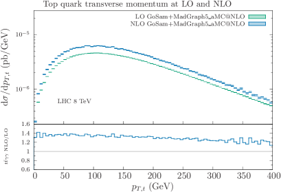
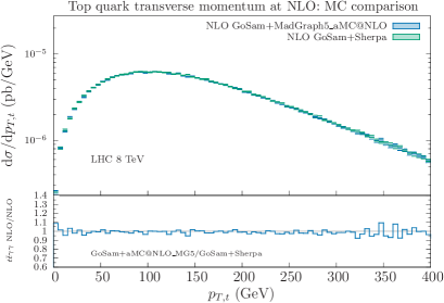
Figure 1: Transverse momentum of the top quark in $pp\to t\bar{t}\gamma\gamma$ for the LHC at 8 TeV: LO and NLO distributions for the transverse momentum of the top quark (left) and NLO comparison between GoSam+MG5_aMC and GoSam+Sherpa (right).

As an application of this novel framework, we computed the NLO QCD corrections to $pp\to$ $t\bar{t}H$ and $pp\to$ $t\bar{t}\gamma\gamma$ matched to a parton shower [35]. The study is performed using NLO predictions for $t\bar{t}H$ and continuum $t\bar{t}\gamma\gamma$ production. The top and anti-top quarks are subsequently decayed semi-leptonically with MadSpin [37], taking into account spin correlation effects, and then showered and hadronised by means of Pythia 8.2 [38]. We compared several distributions to disentangle the two processes and focused in particular on observables designed to study spin correlation effects. While NLO corrections are sizable and provide a clear reduction of theoretical uncertainties, they only mildly distort the shape of the various distributions.

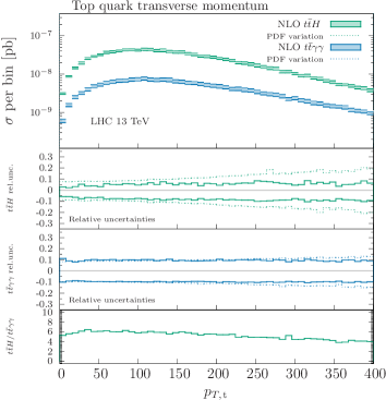
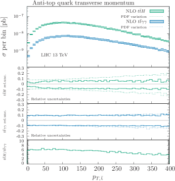
Figure 2: Transverse momentum of the top and anti-top quark in $pp\to t\bar{t}\gamma\gamma$ for the LHC at 13 TeV.

While GoSam was initially designed and developed to compute one-loop virtual contributions needed by NLO predictions, several of it features can be adapted and extended to address specific tasks needed by higher order calculations. Concerning the generation virtual two-loop matrix elements, the routines in GoSam  have been extended [39] to produce the full list and expressions for all two-loop Feynman diagrams contributing to any process: as for the one-loop case, the code depicts all contributing diagrams as output on file, takes care of the algebra by means of form, and projects the expressions over the appropriate tensor structures, to extract the form factors. Interfaces to codes for the reduction to master integrals are also available. The code had been successfully employed for the evaluation of the two-loop virtual amplitudes needed by the evaluation of Higgs boson pair production in gluon fusion at NLO, where relevant master integrals have been computed numerically by means of SecDec-3.0 [40]. More details about this important result have been presented at this conference by Stephen Jones and Matthias Kerner.

As a last application beyond NLO, GoSam has been used for the evaluation of $pp\ \to t\bar{t}H$ and $pp\ \to t\bar{t}W$ at approximate NNLO in QCD [41]. In these papers, approximate formulas were obtained by studying soft-gluon corrections in the limit where the invariant mass of the final state approaches the partonic center-of-mass energy. No assumptions are made about the invariant mass of the final state. The approximate NNLO corrections are extracted from the perturbative information contained in a soft-gluon resummation formula valid to NNLL accuracy, whose derivation is based on SCET (for a recent review, see [42]).

The soft-gluon resummation formula for this process contains three essential ingredients, all of which are matrices in the color space needed to describe four-parton scattering: a hard function, related to virtual corrections; a soft function, related to real emission corrections in the soft limit; and a soft anomalous dimension, which governs the structure of the all-order soft-gluon corrections through the renormalization group (RG). Of these three ingredients, both the NLO soft function [43] and NNLO soft anomalous dimension [44] needed for NNLL resummation in processes involving two massless and two massive partons can be adapted directly to $t\bar{t}H$ and $t\bar{t}W$ production. The NLO hard function is instead process dependent and it was evaluated by using a modified version of the one-loop providers GoSam, MadLoop, and OpenLoops [45].

5 Conclusions

Integrand-reduction techniques played an important role in the automation of NLO calculations. Algorithms such as the four-dimensional integrand-level OPP reduction, $D$-dimensional integrand reduction, integrand reduction via Laurent expansion, embedded in multi-purpose codes interfaced within Monte Carlo tools, allowed to compute cross sections and distributions for a wide variety of processes at NLO accuracy, as needed by the LHC experimental collaborations.

However, integrand reduction did not merely provide a set of numerical and computational algorithms to extract coefficients, but a different approach to scattering amplitudes, based on the study of the general structure of the integrand of Feynman integrals. The advances during past decade also showed that a better understanding of the mathematical properties of scattering amplitudes goes together with the ability of developing efficient algorithms for their evaluation. Moreover, there is still room for improvement, even at NLO.

Will integrand reduction be competitive at NNLO? The challenges and additional complexity presented by NNLO calculations required an extension of integrand reduction techniques to go beyond the current understanding. The language of algebraic geometry provided an ideal framework to determine the functional form of all residues, and attempts of optimizing and reducing the number of terms generated by the integrand decomposition have been presented and will be soon implemented in computational codes. More work is still needed, but integrand reduction might provide an alternative path for NNLO processes with more than two particles in the final state.

Acknowledgments

The results presented in this paper are the outcome of the team work with several talented and motivated collaborators. I would like to thank the present and former members of the GoSam Collaboration for their many contributions. I am particularly indebted with Pierpaolo Mastrolia, Gionata Luisoni, and Tiziano Peraro, for everything I learned from our discussions and common projects. I would also like to thank Alessandro Broggio, William Bobadilla, Andrea Ferroglia, Valentin Hirschi, Amedeo Primo, and Ray Sameshima for stimulating discussions on a wide variety of topics over the past year. Work supported in part by the National Science Foundation under Grants PHY-1068550 and PHY-1417354 and by the PSC-CUNY Awards No. 67536-00 45 and No. 68687-00 46.

References

- [1] Ossola G, Papadopoulos C G and Pittau R 2007 Nucl.Phys. B763 147–169 (Preprint hep-ph/0609007)
- [2] Bern Z, Dixon L J and Kosower D A 2007 Annals Phys. 322 1587–1634 (Preprint 0704.2798); Ellis R K, Kunszt Z, Melnikov K and Zanderighi G 2012 Phys.Rept. 518 141–250 (Preprint 1105.4319); Ossola G 2014 J.Phys.Conf.Ser. 523 012040 (Preprint 1310.3214); Mastrolia P 2015 (Preprint 1507.03226)
- [3] Badger S, Mogull G and Peraro T 2016 (Preprint 1607.00311); Ita H 2016 (Preprint 1607.00705); Febres Cordero F and Ita H 2016 (Preprint 1607.00395); Larsen K J and Zhang Y 2016 (Preprint 1606.09447); Mastrolia P, Peraro T, Primo A and Torres Bobadilla W J 2016 (Preprint 1607.05156); Worek M 2016 (Preprint 1607.01532)
- [4] Passarino G and Veltman M J G 1979 Nucl. Phys. B160 151; ’t Hooft G and Veltman M 1979 Nucl.Phys. B153 365–401
- [5] van Oldenborgh G 1991 Comput.Phys.Commun. 66 1–15; Hahn T and Perez-Victoria M 1999 Comput.Phys.Commun. 118 153–165 (Preprint hep-ph/9807565); Ellis R K and Zanderighi G 2008 JHEP 02 002 (Preprint 0712.1851); van Hameren A 2011 Comput.Phys.Commun. 182 2427–2438 (Preprint 1007.4716); Cullen G, Guillet J, Heinrich G, Kleinschmidt T, Pilon E et al. 2011 Comput.Phys.Commun. 182 2276–2284 (Preprint 1101.5595)
- [6] del Aguila F and Pittau R 2004 JHEP 0407 017 (Preprint hep-ph/0404120)
- [7] Mastrolia P and Ossola G 2011 JHEP 1111 014 (Preprint 1107.6041)
- [8] Badger S, Frellesvig H and Zhang Y 2012 JHEP 1204 055 (Preprint 1202.2019)
- [9] Zhang Y 2012 JHEP 1209 042 (Preprint 1205.5707)
- [10] Mastrolia P, Mirabella E, Ossola G and Peraro T 2012 Phys.Lett. B718 173–177 (Preprint 1205.7087)
- [11] Badger S, Frellesvig H and Zhang Y 2012 JHEP 1208 065 (Preprint 1207.2976)
- [12] Mastrolia P, Mirabella E, Ossola G and Peraro T 2013 Phys.Lett. B727 532–535 (Preprint 1307.5832)
- [13] Kleiss R H, Malamos I, Papadopoulos C G and Verheyen R 2012 JHEP 1212 038 (Preprint 1206.4180); Feng B and Huang R 2013 JHEP 1302 117 (Preprint 1209.3747); Mastrolia P, Mirabella E, Ossola G and Peraro T 2013 Phys.Rev. D87 085026 (Preprint 1209.4319); Søgaard M and Zhang Y 2013 JHEP 12 008 (Preprint 1310.6006); Søgaard M and Zhang Y 2015 Phys. Rev. D91 081701 (Preprint 1412.5577); Søgaard M and Zhang Y 2014 JHEP 12 006 (Preprint 1406.5044); Søgaard M and Zhang Y 2014 JHEP 07 112 (Preprint 1403.2463); Feng B, Zhen J, Huang R and Zhou K 2014 JHEP 06 166 (Preprint 1401.6766); Ita H 2015 (Preprint 1510.05626); Badger S, Mogull G, Ochirov A and O’Connell D 2015 JHEP 10 064 (Preprint 1507.08797); Larsen K J and Zhang Y 2016 Phys. Rev. D93 041701 (Preprint 1511.01071); Badger S, Mogull G and Peraro T 2016 (Preprint 1606.02244)
- [14] Mastrolia P, Peraro T and Primo A 2016 (Preprint 1605.03157)
- [15] Kallen G and Toll J 1965 J. Math. Phys. 6 299–303; Melrose D B 1965 Nuovo Cim. 40 181–213
- [16] Britto R, Cachazo F and Feng B 2005 Nucl. Phys. B725 275–305 (Preprint hep-th/0412103)
- [17] Ossola G, Papadopoulos C G and Pittau R 2007 JHEP 0707 085 (Preprint 0704.1271); Ossola G, Papadopoulos C G and Pittau R 2008 JHEP 0805 004 (Preprint 0802.1876)
- [18] Ossola G, Papadopoulos C G and Pittau R 2008 JHEP 03 042 (Preprint 0711.3596)
- [19] Draggiotis P, Garzelli M, Papadopoulos C and Pittau R 2009 JHEP 0904 072 (Preprint 0903.0356); Garzelli M, Malamos I and Pittau R 2011 JHEP 1101 029 (Preprint 1009.4302); Garzelli M and Malamos I 2011 Eur.Phys.J. C71 1605 (Preprint 1010.1248); Page B and Pittau R 2013 JHEP 1309 078 (Preprint 1307.6142)
- [20] Ellis R K, Giele W T and Kunszt Z 2008 JHEP 03 003 (Preprint 0708.2398); Giele W T, Kunszt Z and Melnikov K 2008 JHEP 0804 049 (Preprint 0801.2237); Ellis R, Giele W T, Kunszt Z and Melnikov K 2009 Nucl.Phys. B822 270–282 (Preprint 0806.3467)
- [21] Mastrolia P, Ossola G, Reiter T and Tramontano F 2010 JHEP 1008 080 (Preprint 1006.0710)
- [22] Melnikov K and Schulze M 2010 Nucl.Phys. B840 129–159 (Preprint 1004.3284)
- [23] Mastrolia P, Ossola G, Papadopoulos C and Pittau R 2008 JHEP 0806 030 (Preprint 0803.3964)
- [24] Mastrolia P, Mirabella E and Peraro T 2012 JHEP 1206 095 (Preprint 1203.0291)
- [25] Peraro T 2014 Comput.Phys.Commun. 185 2771–2797 (Preprint 1403.1229)
- [26] van Deurzen H, Luisoni G, Mastrolia P, Mirabella E, Ossola G et al. 2014 JHEP 1403 115 (Preprint 1312.6678)
- [27] van Deurzen H, Luisoni G, Mastrolia P, Mirabella E, Ossola G et al. 2013 Phys.Rev.Lett. 111 171801 (Preprint 1307.8437)
- [28] Cullen G, van Deurzen H, Greiner N, Luisoni G, Mastrolia P et al. 2013 Phys.Rev.Lett. 111 131801 (Preprint 1307.4737); Greiner N, Höche S, Luisoni G, Schönherr M, Winter J C and Yundin V 2016 JHEP 01 169 (Preprint 1506.01016)
- [29] Hirschi V and Peraro T 2016 JHEP 06 060 (Preprint 1604.01363)
- [30] Hirschi V, Frederix R, Frixione S, Garzelli M V, Maltoni F et al. 2011 JHEP 1105 044 (Preprint 1103.0621)
- [31] Alwall J, Frederix R, Frixione S, Hirschi V, Maltoni F et al. 2014 JHEP 1407 079 (Preprint 1405.0301)
- [32] Cullen G, Greiner N, Heinrich G, Luisoni G, Mastrolia P et al. 2012 Eur.Phys.J. C72 1889 (Preprint 1111.2034); Cullen G, van Deurzen H, Greiner N, Heinrich G, Luisoni G et al. 2014 Eur.Phys.J. C74 3001 (Preprint 1404.7096)
- [33] Nogueira P 1993 J.Comput.Phys. 105 279–289; Vermaseren J A M 2000 (Preprint math-ph/0010025); Reiter T 2010 Comput.Phys.Commun. 181 1301–1331 (Preprint 0907.3714); Cullen G, Koch-Janusz M and Reiter T 2011 Comput.Phys.Commun. 182 2368–2387 (Preprint 1008.0803); Kuipers J, Ueda T, Vermaseren J and Vollinga J 2013 Comput.Phys.Commun. 184 1453–1467 (Preprint 1203.6543)
- [34] Binoth T, Guillet J P, Heinrich G, Pilon E and Reiter T 2009 Comput.Phys.Commun. 180 2317–2330 (Preprint 0810.0992); Heinrich G, Ossola G, Reiter T and Tramontano F 2010 JHEP 1010 105 (Preprint 1008.2441); Guillet J P, Heinrich G and von Soden-Fraunhofen J F 2014 Comput. Phys. Commun. 185 1828–1834 (Preprint 1312.3887)
- [35] van Deurzen H, Frederix R, Hirschi V, Luisoni G, Mastrolia P and Ossola G 2015 (Preprint 1509.02077)
- [36] van Deurzen H 2015 Ph.D. Thesis (Preprint https://mediatum.ub.tum.de/?id=1252703)
- [37] Frixione S, Laenen E, Motylinski P and Webber B R 2007 JHEP 04 081 (Preprint hep-ph/0702198); Artoisenet P, Frederix R, Mattelaer O and Rietkerk R 2013 JHEP 1303 015 (Preprint 1212.3460)
- [38] Sjöstrand T, Ask S, Christiansen J R, Corke R, Desai N, Ilten P, Mrenna S, Prestel S, Rasmussen C O and Skands P Z 2015 Comput. Phys. Commun. 191 159–177 (Preprint 1410.3012)
- [39] Borowka S, Heinrich G, Jahn S, Jones S P, Kerner M, Schlenk J and Zirke T 2016 (Preprint 1604.00267); Borowka S, Greiner N, Heinrich G, Jones S, Kerner M, Schlenk J, Schubert U and Zirke T 2016 Phys. Rev. Lett. 117 012001 (Preprint 1604.06447)
- [40] Borowka S, Heinrich G, Jones S P, Kerner M, Schlenk J and Zirke T 2015 Comput. Phys. Commun. 196 470–491 (Preprint 1502.06595)
- [41] Broggio A, Ferroglia A, Pecjak B D, Signer A and Yang L L 2016 JHEP 03 124 (Preprint 1510.01914); Broggio A, Ferroglia A, Ossola G and Pecjak B D 2016 (Preprint 1607.05303)
- [42] Becher T, Broggio A and Ferroglia A 2014 (Preprint 1410.1892)
- [43] Ahrens V, Ferroglia A, Neubert M, Pecjak B D and Yang L L 2010 JHEP 09 097 (Preprint 1003.5827); Li H T, Li C S and Li S A 2014 Phys. Rev. D90 094009 (Preprint 1409.1460)
- [44] Ferroglia A, Neubert M, Pecjak B D and Yang L L 2009 Phys. Rev. Lett. 103 201601 (Preprint 0907.4791); Ferroglia A, Neubert M, Pecjak B D and Yang L L 2009 JHEP 11 062 (Preprint 0908.3676)
- [45] Cascioli F, Maierhofer P and Pozzorini S 2012 Phys.Rev.Lett. 108 111601 (Preprint 1111.5206)