Exploring the “Middle Earth” of Network Spectra via a Gaussian Matrix Function

Abstract

We study a Gaussian matrix function of the adjacency matrix of artificial and real-world networks. In particular, we study the Gaussian Estrada index—an index characterizing the importance of eigenvalues close to zero. This index accounts for the information contained in the eigenvalues close to zero in the spectra of networks. Here we obtain bounds for this index in simple graphs, proving that it reaches its maximum for star graphs followed by complete bipartite graphs. We also obtain formulas for the Estrada Gaussian index of Erdős-Rï¿œnyi random graphs as well as for the Barabï¿œsi-Albert graphs. We also show that in real-world networks this index is related to the existence of important structural patterns, such as complete bipartite subgraphs (bicliques). Such bicliques appear naturally in many real-world networks as a consequence of the evolutionary processes giving rise to them. In general, the Gaussian matrix function of the adjacency matrix of networks characterizes important structural information not described in previously used matrix functions of graphs.

The spectrum of a network—the set of its eigenvalues—provides important information about the structural and dynamical properties of the corresponding system. Most of the functions used to study network spectra give more weight to the largest modular eigenvalues. Then, the information contained in the eigenvalues close to the centre of the spectra, i.e, those close to zero, has remained totally unexplored in the study of graph spectra. Here we study a Gaussian matrix function that gives more weights to the eigenvalues closest to the centre of the spectrum of a network. Using this function we extract important structural information hidden in the spectra of networks, such as emergence of complete bipartite subgraphs (bicliques) which appear naturally in many real-world networks as a consequence of the evolutionary processes giving rise to them. These bicliques are also ubiquitous in random networks generated by preferential attachment mechanisms, such as the Barabï¿œsi-Albert model. In this work we provide a series of analytical results that pave the way for further analysis and uses of this Gaussian matrix function to understand network structure and dynamics.

I Introduction

Matrix functions Function of matrices have emerged as an important mathematical tool for studying networks Estrada Higham . The concepts of communicability Communicability , subgraph centrality Protein folding ; Subgraph Centrality (see also Estrada Hatano Benzi for a review) and Katz index Katz centrality are derived from matrix functions $f\left(A\right)$ of the adjacency matrix and allow the characterization of local structural properties of networks. The trace of $f\left(A\right)$, which is known as the Estrada index of the graph Estrada index ; Estrada index 1 ; Estrada index 2 , is a useful characterization of the global structure of a graph and it has found applications as an index of natural connectivity for studying robustness of networks Natural connectivity 1 ; Natural connectivity 2 . These initial studies have motivated more recent developments in the theory of graph-theoretic matrix function studies Benzi 1 ; Benzi 2 ; Benzi 3 . All these indices have found multiple applications for studying real-world social, ecological, biological, infrastructural, and technological systems represented by networks Michaelbook ; EstradaBook ; LucianoReview . Here we will use interchangeably the terms networks and graphs and will follow standard notation as in EstradaBook . The greatest appeal of the use of functions of the adjacency matrix for studying graphs is that when representing them in terms of a Taylor function expansion: $f\left(A\right)=\sum_{k=0}^{\infty}c_{k}A^{k}$, the entries of the $k$th power of the adjacency matrix provides information about the number of walks of length $k$ between the corresponding pair of (not necessarily different) nodes (see next section for formal definitions). Then, the important ingredient of the definition of $f\left(A\right)$ lies in the use of the coefficients $c_{k}$. The use of $c_{k}=k!^{-1}$ gives rise to the exponential function of the adjacency matrix, which is the basis of the communicability/subgraph centrality. On the other hand, selecting $c_{k}=\alpha^{-k}$ gives rise to the resolvent of the adjacency matrix, which is the basis of the Katz centrality index Katz centrality . Either of these two coefficients is selected arbitrarily among all the existing possibilities. However, they have proved to be very useful in practice and not very much improvement is obtained by changing the coefficients to account for bigger or smaller penalization of the walks according to their length Zooming in and out .

Here we propose to investigate the information contained in the mid part of the spectrum of the adjacency matrix of graphs and networks using a new adjacency matrix function. The adjacency matrix of a simple graph always contains positive and negative eigenvalues. Then, we will refer here to the region close to the zero eigenvalue as the middle part of the spectrum. This is only truly the middle part in bipartite networks where the spectrum is symmetric, but we will use the term without loss of generality for any graph. This region of the spectrum is totally unexplored for complex networks. However, there are areas in which the zero eigenvalue plays a fundamental role. For instance, when the adjacency matrix represents the tight-binding Hamiltonian in the Hï¿œckel molecular orbital (HMO) method (see HMO_1 ; HMO_2 for recent reviews), the zero eigenvalue and its multiplicity (graph nullity) represent important parameters related to the molecular stability and molecular magnetic properties (see Graph nullity review for a review). In these cases the highest occupied (HOMO) and lowest unoccupied molecular orbitals (LUMO), which correspond to the smallest positive and the smallest negative eigenvalue of $A$, respectively, play the most fundamental role in the chemical reactivity. It can be said that everything interesting in Chemistry takes place with the involvement of the eigenvalues closest to zero. For instance, many chemical reactions and electron transfer complexes involve electron transfers between the HOMO of one molecule and the LUMO of another Fukui ; Fukui_2 ; Frontiers orbitals .

Matrix functions of the type of $f\left(A\right)=\sum_{k=0}^{\infty}c_{k}A^{k}$ are characterized by the fact that they give the highest weight to the largest eigenvalue of the adjacency matrix. For a simple example let us consider the trace of $f\left(A\right)=\exp\left(A\right)$ of a simple, connected network, which can be written as $tr\exp\left(A\right)=\sum_{j=1}^{n}\exp\left(\lambda_{j}\right)$, where $n$ is the order of the graph and $\lambda_{1}>\lambda_{2}\geq\cdots\geq\lambda_{n}$ are the eigenvalues of $A$. It is clear that if the spectral gap of the adjacency matrix, $\lambda_{1}-\lambda_{2}$, is very large, $tr\exp\left(A\right)$ depends only of the largest eigenvalue $\lambda_{1}$. This is not a strange situation in real-world networks, where it is typical to find very large spectral gaps for their adjacency matrix. In these cases the use of functions of the type $f\left(A\right)$ makes that the structural information contained in the smaller eigenvalues and eigenvectors of the adjacency matrix is not captured by the index. A similar situation happens if we consider $f\left(-A\right)$ Negative temperature . In this case we give more weight to the smallest eigenvalue/eigenvector of the adjacency matrix and the information contained in the largest ones is again lost.

In this work we study a Gaussian adjacency matrix function $f\left(-A^{2}\right)$ as a way to characterize the structural information of graphs giving more importance to the eigenvalues/eigenvectors in the middle part of the graph spectrum. Similar Gaussian operators may arise in quantum mechanics of many body systems Gaussian operator 1 ; Gaussian operator 2 as well as as the electronic partition function in renormalized tight binding Hamiltonians renormalized ; Estrada Benzi Gaussian . We start by proving some elementary results for some of the indices derived from $f\left(-A^{2}\right)$ for general graphs. In particular we study here properties of $H=trf\left(-A^{2}\right)$. We show that although the graph nullity—the multiplicity of the zero eigenvalue of the adjacency matrix of the graph—plays an important role in the values of this index, the $H$ index contains more structural information than the graph nullity even for small simple graphs. We then prove that among the graphs with $n$ nodes, the maximum of the $H$ index is always obtained for the star graph followed by other complete bipartite graphs. Then, we obtain analytic expressions for this index in random graphs with Poisson and power-law degree distribution, showing that the last ones always display larger values of the $H$ index than the first ones. Finally, we study more than 60 real-world networks representing a large variety of complex systems. In this case we study the $H$ index normalized by the network size, $\hat{H}$. We found that the networks with the largest $\hat{H}$ index correspond to those having relatively large bicliques—complete bipartite subgraphs, which can be created by different evolutionary mechanisms depending on the kind of complex system considered. Although there are important network characteristics influencing the $\hat{H}$ index, such as degree distribution and the degree assortativity, we show here that they are not unique in determining the high values of this index observed for certain networks. This new matrix function for graphs and networks may represent an important addition to the characterization of important properties of these systems which have remained unexplored due to the lack of characterizations of the ’middle region’ of graph spectra.

II Preliminaries

Let us introduce some definitions, notations, and properties associated with networks to make this work self-contained. We will use interchangeably the terms graphs and networks in this work. A graph $\Gamma=(V,E)$ is defined by a set of $n$ nodes (vertices) $V$ and a set of $m$ edges $E=\{(u,v)|u,v\in V\}$ between the nodes. Here we will consider simple graphs without multiple edges, self-loops and direction of the edges. A walk of length $k$ in $G$ is a set of nodes $i_{1},i_{2},\ldots,i_{k},i_{k+1}$ such that for all $1\leq l\leq k$, $(i_{l},i_{l+1})\in E$. A closed walk is a walk for which $i_{1}=i_{k+1}$. A path is a walk with no repeated nodes.

Let $A$ be the adjacency operator on $\ell_{2}(V)$, namely $(Af)(p)=\sum_{q:{\rm dist}(p,q)=1}f(q)$ . For simple finite graphs $A$ is the symmetric adjacency matrix of the graph, which has entries

$$a_{uv}=\left\{\begin{array}[]{ll}1&\mbox{if }(u,v)\in E\\ 0&\mbox{otherwise}\end{array}\right.\qquad\forall u,v\in V.$$

The degree $k_{i}$ of the node $i$ is the number of edges incident to it, equivalently $k_{i}=\sum_{j}a_{ij}$. In the particular case of an undirected network as the ones studied here, the associated adjacency matrix is symmetric, and thus its eigenvalues are real. We label the eigenvalues of $A$ in non-increasing order: $\lambda_{1}>\lambda_{2}\geq\ldots\geq\lambda_{n}$. Since $A$ is a real-valued, symmetric matrix, we can decompose $A$ into $A=U\Lambda U^{T}$ where $\Lambda$ is a diagonal matrix containing the eigenvalues of $A$ and $U=[\mathbf{\overrightarrow{\psi}}_{1},\ldots,\mathbf{\overrightarrow{\psi}}_{n}]$ is orthogonal, where $\mathbf{\overrightarrow{\psi}}_{i}$ is an eigenvector associated with $\lambda_{i}$. Because the graphs considered here are connected, $A$ is irreducible and from the Perron-Frobenius theorem we can deduce that $\lambda_{1}>\lambda_{2}$ and that the leading eigenvector $\mathbf{q}_{1}$, which will be sometimes referred to as the Perron vector, can be chosen such that its components $\mathbf{\mathbf{\overrightarrow{\psi}}}_{1}(u)$ are positive for all $u\in V$.

Hereafter we will refer to the following function as the communicability function of the graph Communicability ; Estrada Higham ; Estrada Hatano Benzi . Let $u$ and $v$ be two nodes of $\Gamma$. The communicability function between these two nodes is defined as

$$G_{uv}=\sum_{k=0}^{\infty}\frac{\left(A^{k}\right)_{uv}}{k!}=\left(\exp\left(A\right)\right)_{uv}=\sum_{k=1}^{n}e^{\lambda_{k}}\mathbf{\mathbf{\overrightarrow{\psi}}}_{k}(u)\mathbf{\overrightarrow{\psi}}_{k}(v),$$

which is an important quantity for studying communication processes in networks. It counts the total number of walks starting at node $u$ and ending at node $v$, weighted in decreasing order of their length by a factor $\frac{1}{k!}$; therefore it is considering shorter walks more influential than longer ones. The $G_{uu}$ terms of the communicability function characterize the degree of participation of a node in all subgraphs of the network, giving more weight to the smaller ones. Thus, it is known as the subgraph centrality of the corresponding node Subgraph Centrality . The following quantity is known in the algebraic graph theory literature as the Estrada index of the graph:

$$EE\left(G\right)=\sum_{u=1}^{n}G_{uu}=tr\left(\exp\left(A\right)\right)=\sum_{k=1}^{n}e^{\lambda_{k}},$$

which is a characterization of the global properties of a network. In its generalized form $EE\left(G,\beta\right)=tr\left(\exp\left(\beta A\right)\right)=\sum_{k=1}^{n}e^{\beta\lambda_{k}},$ it represents the statistical-mechanics partition function of the graph where $\beta$ represents the inverse temperature.

In some parts of this work we will consider the following integral

$$I_{\gamma}(x)=\frac{1}{\pi}\stackrel{{\scriptstyle[}}{{0}}]{\pi}{\int}\cos(\gamma\theta)\exp(x\cos\theta)d\theta-\frac{\sin(\gamma\pi)}{\pi}\stackrel{{\scriptstyle[}}{{0}}]{\infty}{\int}\exp(-x\cosh t-\gamma t)dt,$$ (1)

which corresponds to the modified Bessel function of the first kind.

III Gaussian Adjacency Matrix Function of Networks

With the goal of accounting for the influence of the eigenvalues close to middle of the spectrum of the adjacency matrix of a graph, i.e., those close to zero, we start here by introducing the following matrix function

$$\tilde{G}=\sum_{k=0}^{\infty}\dfrac{\left(-A^{2}\right)^{k}}{k!}=\exp(-A^{2}).$$ (2)

By obvious reasons we will call it the Gaussian matrix function of $A$. Let $\tilde{G}_{pq}$ be the Gaussian communicability function between the nodes $p$ and $q$ based on $-A^{2}$. That is,

$$\tilde{G}_{pq}=(\exp(-A^{2}))_{pq}$$ (3)

Correspondingly, $\tilde{G}_{pp}$ is the Gaussian subgraph centrality based on the same matrix function. The trace of $\exp(-A^{2})$ will be designated by

$$H=tr(\exp(-A^{2})),$$ (4)

which corresponds to the Gaussian Estrada index of the graph. It is very important to mention that for calculating the index $H$ we do not need to obtain explicitly the exponential matrix of $-A^{2}$. We are not interested here in the development of such kind of techniques but the reader is directed to the excellent work of Benzi and Boito Benzi_Boito for a discussion of efficientￜ techniques for estimating the trace of an exponential matrix that do not require computing every entry of the matrix exponential.ￜ

Obviously, using the spectral decomposition of the adjacency matrix we can express both indices as

$$\tilde{G}_{pq}=\sum_{j=1}^{n}\psi_{j,p}\psi_{j,q}\exp\left(-\lambda_{j}^{2}\right),$$ (5)

$$H=\sum_{j=1}^{n}\exp\left(-\lambda_{j}^{2}\right).$$ (6)

Let $\eta\left(A\right)$ be the nullity of the adjacency matrix $A$, i.e., the dimension of the null space of $A$. In spectral graph theory $\eta=\eta\left(A\right)$ is known as the graph nullity. Then, it is obvious that the $H$ index is related to $\eta$ as follows:

$$H\geq\eta,$$ (7)

with both indices identical if and only if $\lambda_{j}=0$, for all $j$, which is attained only for the trivial graph, i.e., the graph with $n$ nodes and no edges. Indeed,

$$H=\eta+\sum_{\lambda_{j}\neq 0}\exp\left(-\lambda_{j}^{2}\right).$$ (8)

Then, it is interesting at least empirically, to explore the relation between $H$ and $\eta$ for simple graphs. We investigate all the connected graphs with $n\leq 8$ for which we obtain both $H$ and $\eta$. The correlation between both indices for the 11,117 connected graphs with 8 nodes is illustrated in Figure (1). Although the correlation is statistically significant—the Pearson correlation coefficient is 0.74—it hides the important differences between the two indices. For instance, there are 5,724 graphs with zero nullity among all the connected graphs with 8 nodes. For these graphs $1.484\leq H\leq 3.629$, which represents a wide range of values taking into account that the minimum and maximum values of $H$ for all connected graphs with 8 nodes are 1.484 and 6, respectively. It is also easy to see that there are graphs having nullity zero which have larger $H$ indices than some graphs having nullity one, two or three. The results are very similar for $n<8$ and they are not shown here. In the Figure (1) we show the graphs with the largest $H$ indices among all connected graphs with 8 nodes and nullity zero or one. These graphs show a common pattern containing several complete bipartite subgraphs. For instance, every yellow node in the Figure (1) is connected to every red ones, every red is connected to every blue and every blue is connected to the green one, while there is no yellow-yellow, red-red or blue-blue connections. This pattern will be revealed when we study the mathematical properties of this index and its importance will be analyzed for real-world networks.

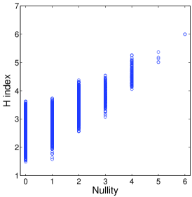
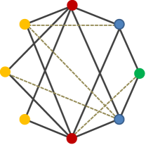
(a) (b) (c)

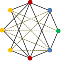
Figure 1: (a) Plot of graph nullity versus $H$ index for all connected graphs with 8 nodes. (b) Graph with the largest $H$ index among all the connected graphs with 8 nodes and nullity zero. (c) The same as in (b) for all connected graphs with nullity one. Notice in (b) and (c) the connectivity pattern of the graphs in which every yellow node is connected to every red ones, every red is connected to every blue and every blue is connected to the green one. Also, there is no yellow-yellow, red-red or blue-blue connections.

III.1 General Quadrature Rule-Based Bounds

In this section we will use the Gaussian quadrature rule to obtain an upper bound of $H$. We will mainly follow here the works quadrature rule 1 ; quadrature rule 2 ; quadrature rule 3 to which the reader is directed for more. We start by recalling that for a symmetric matrix $A$ and a smooth function $f$ defined on an interval containing the eigenvalues of $A,\left[a,b\right]$ we have:

$$I\left[f\right]=u^{T}f(A)v=\stackrel{{\scriptstyle[}}{{b}}]{a}{\int}f(\lambda)d\mu(\lambda)\textnormal{ where }\mu(\lambda)=\begin{cases}0,&\lambda\lneq a=\lambda_{1}\\ \stackrel{{\scriptstyle[}}{{j}}=1]{i}{\sum}p_{j}q_{j,}&\lambda_{i}\leq\lambda\lneq\lambda_{i+1}\\ \stackrel{{\scriptstyle[}}{{j}}=1]{N}{\sum}p_{j}q_{j,}&b=\lambda_{n}\leq\lambda.\end{cases}$$ (9)

Our motivation for using this definition is the fact that $\left[f(A)\right]_{ij}=e_{i}^{T}f(A)e_{j}$, where $e_{i}$ is the $i$th column of the identity matrix. Moreover, $u^{T}f(A)v=\stackrel{{\scriptstyle[}}{{b}}]{a}{\int}f(\lambda)d\mu(\lambda)=\stackrel{{\scriptstyle[}}{{j}}=1]{n}{\sum}w_{j}f(t_{j})+\stackrel{{\scriptstyle[}}{{k}}=1]{M}{\sum}v_{k}f(z_{k})+R\left[f\right]$ which is the general Gauss-type quadrature rule where the nodes $\left\{t_{j}\right\}_{j=1}^{n}$ and wights $\left\{w_{j}\right\}_{j=1}^{n}$ are unknowns, whereas the nodes $\left\{z_{k}\right\}_{k=1}^{M}$ are prescribed . We have:

• $M=0$ for the Gauss rule,

• $M=1$, $z_{1}=a$ or $z_{1}=b$ for the Gauss-Radau rule,

• $M=2$, $z_{1}=a$ and $z_{2}=b$ for the Gauss-Lobatto rule, which we will focus on.

Let $J_{n}$ be a tridiagonal matrix defined as

$$J_{n}=\left[\begin{array}[]{ccccc}\omega_{1}&\gamma_{1}\\ \gamma_{1}&\omega_{2}&\gamma_{2}\\ &\ddots&\ddots&\ddots\\ &&\gamma_{n-2}&\omega_{n-1}&\gamma_{n-1}\\ &&&\gamma_{n-1}&\omega_{n}\end{array}\right],$$

whose eigenvalues are the Gauss nodes, whereas the Gauss wights are given by the square of the first entries of the normalized eigenvectors of $J_{n}$, then,

$$\stackrel{{\scriptstyle[}}{{l}}=1]{N}{\sum}w_{l}f(t_{l})=e_{1}^{T}f(J_{n})e_{1}.$$ (10)

The entries of $J_{n}$ are computed using the symmetric Lanczos algorithm. Now, if $f$ is a strictly completely monotonic function on an interval $I=[a,b]$ containing the eigenvalues of the matrix $A$, i.e $f^{(2j)}(x)>0$ and $f^{(2j+1)}(x)<0$ on $I$ for all $j\geq 0$ where $f^{(k)}$ denotes the $k$th derivative of $f$ and $f^{(0)}\equiv f$, the symmetric Lanczos process can be used to compute bounds for the diagonal entries $(f(A))_{ii}$. Let $J_{2}=\left[\begin{array}[]{cc}\omega_{1}&\gamma_{1}\\ \gamma_{1}&\omega_{2}\end{array}\right]$ be the Jacobian matrix obtained by taking a single Lanczos step, then we only need to compute the $(1,1)$ entry of $f(J_{2})$. Now, if $\varphi(x,y)=\frac{\omega_{1}\left(f(x)-f(y)\right)+xf(y)-yf(x)}{x-y}$, then the Gauss-Lobatto rule gives the bound

$$(f(A))_{ii}\leq\varphi(a,b).$$

See quadrature rule 1 for more details.

The main result of this section is the following.

Theorem 1.

Let $G$ be a graph with $n$ nodes and $m$ edges and let $H=tr\exp\left(-A^{2}\right)$. Then,

$$H\left(G\right)\leq\stackrel{{\scriptstyle[}}{{i}}=1]{n}{\sum}\left[\frac{d_{i}(e^{-b}-1)}{b}+1\right]=2m\frac{(e^{-b}-1)}{b}+n.$$ (11)

Proof.

In the case of $J_{2}$ we have:

$$J_{2}=\left[\begin{array}[]{cc}\omega_{1}&\gamma_{1}\\ \gamma_{1}&\omega_{2}\end{array}\right],\omega_{1}=a_{ii},\gamma_{1}^{2}=\underset{i\neq j}{\sum}a_{ij}^{2},\omega_{2}=\frac{1}{\gamma_{1}^{2}}\underset{k\neq i}{\sum}\underset{l\neq i}{\sum}a_{ki}a_{kl}a_{li}$$

Now, if $B=A^{2}$, where $A$ is the adjacency matrix of a graph $G$ and $f(x)=e^{-x}$ we have

$$J_{2}=\left[\begin{array}[]{cc}d_{i}&\sqrt{\underset{i\neq j}{\sum}b_{ij}^{2}}\\ \sqrt{\underset{i\neq j}{\sum}b_{ij}^{2}}&\frac{1}{\sqrt{\underset{i\neq j}{\sum}b_{ij}^{2}}}\underset{k\neq i}{\sum}\underset{l\neq i}{\sum}b_{ki}b_{kl}b_{li}\end{array}\right]$$

where $d_{i}$ is the degree of the node $i$ and $b_{ij}$ is the $(i,j)$th entry of $A^{2}$. Notice that $b_{ij}=\stackrel{{\scriptstyle[}}{{k}}=1]{n}{\sum}a_{ik}a_{kj}$ and $\left[a,b\right]=\left[0,b\right]$ since $A^{2}$ has nonnegative eigenvalues.

Hence, we have for the Gauss-Lobatto rule

$$(e^{-A^{2}})_{ii}\leq\frac{d_{i}(1-e^{-b})-b}{-b}=\frac{d_{i}(e^{-b}-1)}{b}+1,$$

To find the bound of the trace of $e^{-A^{2}}$ we take the summation from $1$ to $n$ on the previous inequality, which by the Handshaking Lemma gives the final result. ∎

IV H Index of Graphs

IV.1 Elementary properties

In the following we show some results about $\tilde{G}_{pq}$ of some elementary graphs which will help us to interpret this measure when applied to more complex structures. In particular, we study the $n$-nodes path $P_{n}$, the $n$-nodes cycle $C_{n}$, the star graph $K_{1,n-1}$, the complete graph $K_{n}$ of $n$ nodes and the complete bipartite graph $K_{n_{1},n_{2}}$ of $n_{1}+n_{2}$ nodes. $P_{n}$ is a connected graph in which $n-2$ nodes are connected to other two nodes and two nodes are connected to only one node; $C_{n}$ is the connected graph of $n$ nodes in which every node is connected to two others; $K_{1,n-1}$is the connected graph in which there is one node connected to $n-1$ nodes, here labeled as $1$ and named the central node, and $n-1$ nodes are connected to the central one only; $K_{n}$ is the graph in which every pair of nodes is connected by an edge; and $K_{n_{1},n_{2}}$ is the connected graph which is formed by two sets $V_{1}$ and $V_{2}$ of nodes of cardinalities $n_{1}$ and $n_{2}$, respectively, such that every node in $V_{1}$ is connected to every node in $V_{2}$. Here we give expressions for the $H\left(G\right)$ index of the before mentioned graphs in the form of Lemmas.

Lemma 1.

Let $K_{n}$ be the complete graph of $n$ nodes. Then

$$H\left(K_{n}\right)=e^{-(n-1)^{2}}+\frac{n-1}{e}.$$ (12)

Proof.

The spectrum of $K_{n}$ is $\sigma(K_{n})=\left\{\left[n-1\right]^{1},\left[-1\right]^{n-1}\right\}$ with the eigenvector $\varphi_{1}=\frac{1}{\sqrt{n}}(1,1,\ldots,1)$ so we have

$$\tilde{G}_{pq}\left(K_{n}\right)=\varphi_{1}(p)\varphi_{1}(q)e^{-(n-1)^{2}}+\stackrel{{\scriptstyle[}}{{j}}=2]{n}{\sum}\varphi_{j}(p)\varphi_{j}(q)e^{-1}$$ (13)

And since the eigenvector matrix has orthonormal rows and columns we have $\stackrel{{\scriptstyle[}}{{j}}=2]{n}{\sum}\varphi_{j}(p)\varphi_{j}(q)=-\frac{1}{n}$ if $p\neq q$ and $\frac{n-1}{n}$ if $p=q$.

$$\tilde{G}_{pq}\left(K_{n}\right)=\frac{e^{-(n-1)^{2}}}{n}-\frac{1}{ne}$$ (14)

Now, if $p=q$ then $\tilde{G}_{pp}\left(K_{n}\right)=\varphi_{1}^{2}(p)e^{-(n-1)^{2}}+\stackrel{{\scriptstyle[}}{{j}}=2]{n}{\sum}\varphi_{j}^{2}(p)e^{-1}=\frac{e^{-(n-1)^{2}}}{n}+\frac{n-1}{ne}$.

Then, it is straightforward to realize that

$$H \left(K_{n}\right)= \stackrel{{\scriptstyle[}}{{j}}=1]{n}{\sum}(\frac{e^{-(n-1)^{2}}}{n}+\frac{n-1}{ne})$$ (15)

$$= e^{-(n-1)^{2}}+\frac{n-1}{e}$$ (16)

∎

Lemma 2.

Let $P_{n}$ be a path having $n$ nodes. Then, asymptotically as $n\rightarrow\infty$

$$H\left(P_{n}\right)=\frac{I_{0}(2)}{e^{2}}(n+1)-e^{-4}.$$ (17)

Proof.

By substituting the eigenvalues and eigenvectors of the path graph into the expression for $\tilde{G}_{pp}\left(P_{n}\right)$ we obtain

$$\tilde{G}_{pp}\left(P_{n}\right) = \frac{2}{n+1}\stackrel{{\scriptstyle[}}{{j}}=1]{n}{\sum}\sin^{2}\left(\frac{j\pi p}{n+1}\right)\exp\left(-4\cos^{2}\left(\frac{j\pi}{n+1}\right)\right)$$ (18)

$$= \frac{e^{-2}}{n+1}\stackrel{{\scriptstyle[}}{{j}}=1]{n}{\sum}\left[1-\cos\left(\frac{2j\pi p}{n+1}\right)\right]\exp\left(-2\cos\left(\frac{2j\pi}{n+1}\right)\right).$$ (19)

Now, when $n\rightarrow\infty$ the summation in 19 can be approached by the following integral

$$\tilde{G}_{pp}\left(P_{n}\right)=\frac{e^{-2}}{\pi}\int_{0}^{\pi}\exp(-2\cos\theta)d\theta-\frac{e^{-2}}{\pi}\int_{0}^{\pi}\cos\left(p\theta\right)\exp(-2\cos\theta)d\theta,$$ (20)

where $\theta=\frac{2j\pi}{n+1}$. Thus, when $n\rightarrow\infty$ we have

$$\tilde{G}_{pp}\left(P_{n}\right)=e^{-2}\left(I_{0}(-2)-I_{p}(-2)\right)$$ (21)

which by using $I_{\gamma}(-x)=(-1)^{\gamma}I_{\gamma}(x)$ gives

$$\tilde{G}_{pp} \left(P_{n}\right)= e^{-2}\left(I_{0}(2)-(-1)^{p}I_{p}(2)\right).$$

Let $n$ be even. Then due to the symmetry of the path we have

$$H\left(P_{n}\right) = 2\stackrel{{\scriptstyle[}}{{p}}=1]{n/2}{\sum}\tilde{G}_{pp}\left(P_{n}\right)=2\stackrel{{\scriptstyle[}}{{p}}=1]{n/2}{\sum}e^{-2}\left[I_{0}(2)-(-1)^{p}I_{p}(2)\right]$$ (22)

$$= \frac{nI_{0}(2)}{e^{2}}-\frac{2}{e^{2}}\stackrel{{\scriptstyle[}}{{p}}=1]{n/2}{\sum}(-1)^{p}I_{p}(2).$$ (23)

For $n\rightarrow\infty$ we have

$$\stackrel{{\scriptstyle[}}{{\gamma}}=1]{\infty}{\sum}(-1)^{\gamma}I_{\gamma}(x)=\frac{1}{2}\left(e^{-x}-I_{0}(x)\right).$$ (24)

Then, we can write for $n\rightarrow\infty$

$$H\left(P_{n}\right) = \frac{nI_{0}(2)}{e^{2}}-\frac{1}{e^{2}}\left(e^{-2}-I_{0}(2)\right)$$ (25)

$$= \frac{I_{0}(2)}{e^{2}}(n+1)-e^{-4}.$$ (26)

Now, when $n$ is odd we can split the path into two paths of lengths $\frac{n+1}{2}$ and $\frac{n-1}{2}$, respectively. Then, we write

$$H\left(P_{n}\right) = \stackrel{{\scriptstyle[}}{{p}}=1]{\frac{n+1}{2}}{\sum}\tilde{G}_{pp}\left(P_{n}\right)+\stackrel{{\scriptstyle[}}{{p}}=\frac{n-1}{2}]{n}{\sum}\tilde{G}_{pp}\left(P_{n}\right)$$ (27)

$$= \frac{(n+1)I_{0}(2)}{2e^{2}}-\frac{1}{e^{2}}\stackrel{{\scriptstyle[}}{{p}}=1]{\frac{n+1}{2}}{\sum}(-1)^{p}I_{p}(2)+\frac{(n-1)I_{0}(2)}{2e^{2}}-\frac{1}{e^{2}}\stackrel{{\scriptstyle[}}{{p}}=\frac{n-1}{2}]{n}{\sum}(-1)^{p}I_{p}(2).$$ (28)

When $n\rightarrow\infty$ we can consider that the summation in the second and fourth terms of 28 are both equal to $\left(e^{-2}-I_{0}(2)\right)/2$, which then gives the final result. ∎

Lemma 3.

Let $C_{n}$ be a cycle having $n$ nodes. Then, asymptotically as $n\rightarrow\infty$

$$H(C_{n})=\frac{nI_{0}(-2)}{e^{2}}.$$ (29)

Proof.

(Lemma 3): Notice that the adjacency matrix of a cycle is a circulant matrix and consequently any function of it and that gives

$$H(C_{n}) = \stackrel{{\scriptstyle[}}{{j}}=1]{n}{\sum}\tilde{G}_{pp},\,for\,any\,node\,p$$ (30)

$$= n\left(\frac{tr(e^{-A^{2}})}{n}\right)$$ (31)

$$= n\left(\frac{1}{n}\stackrel{{\scriptstyle[}}{{j}}=1]{n}{\sum}e^{-4\cos^{2}(\frac{2\pi j}{n})}\right)$$ (32)

$$= ne^{-2}\left(\stackrel{{\scriptstyle[}}{{j}}=1]{n}{\sum}\frac{1}{n}e^{-2\cos\frac{4\pi j}{n}}\right)$$ (33)

Now, when $n\rightarrow\infty$ the summation in 33 can be approached by the following integral

$$H(C_{n})=ne^{-2}\frac{1}{\pi}\int_{0}^{\pi}e^{-2cos\theta}d\theta$$ (34)

where $\theta=\frac{2j\pi}{n}$. Thus, when $n\rightarrow\infty$ we have

$$H(C_{n})=ne^{-2}I_{0}(-2).$$ (35)

∎

Lemma 4.

Let $K_{n_{1},n_{2}}$ be the complete bipartite graph of $n_{1}+n_{2}$ nodes. Then

$$H\left(K_{n_{1},n_{2}}\right)=2e^{-n_{1}n_{2}}+n_{1}+n_{2}-2.$$ (36)

The following corollary will be of importance in the following section of this work.

Proof.

(Lemma 4): From the orthonormality of the eigenvectors of the adjacency matrix we have:

$$\stackrel{{\scriptstyle[}}{{j}}=2]{n_{1}+n_{2}-1}{\sum}\left[\varphi_{j}\left(p\right)\right]^{2}=1-\frac{1}{n_{1}},\,p\in V_{1}$$ (37)

$$\stackrel{{\scriptstyle[}}{{j}}=2]{n_{1}+n_{2}-1}{\sum}\left[\varphi_{j}\left(p\right)\right]^{2}=1-\frac{1}{n_{2}},\,p\in V_{2}$$ (38)

Hence, if $p\in V_{1}$

$$\tilde{G}_{pp}\left(K_{n_{1},n_{2}}\right) = \stackrel{{\scriptstyle[}}{{j}}=1]{n_{1}+n_{2}}{\sum}\left[\varphi_{j}\left(p\right)\right]^{2}\exp(-\lambda_{j}^{2})$$ (39)

$$= e^{-n_{1}n_{2}}(\frac{n_{1}n_{2}}{2n_{1}n_{2}^{2}}+\frac{n_{1}n_{2}}{2n_{2}n_{1}^{2}})+\stackrel{{\scriptstyle[}}{{j}}=2]{n_{1}+n_{2}-1}{\sum}\left[\varphi_{j}\left(p\right)\right]^{2}$$ (40)

$$= e^{-n_{1}n_{2}}(\frac{1}{n_{1}})+1-\frac{1}{n_{1}}=\frac{1}{n_{1}}(e^{-n_{1}n_{2}}-1)+1,$$ (41)

and similarly we have $\tilde{G}_{pp}\left(K_{n_{1},n_{2}}\right)=\frac{1}{n_{2}}(e^{-n_{1}n_{2}}-1)+1$ when $p\in V_{2}$. Then

$$H \left(K_{n_{1},n_{2}}\right)= \stackrel{{\scriptstyle[}}{{j}}=1]{n_{1}+n_{2}}{\sum}\tilde{G}_{pp}$$ (42)

$$= \stackrel{{\scriptstyle[}}{{j}}=1]{n_{1}}{\sum}\tilde{G}_{pp}+\stackrel{{\scriptstyle[}}{{j}}=m+1]{n_{1}+n_{2}}{\sum}\tilde{G}_{pp}$$ (43)

$$= n_{1}(\frac{1}{n_{1}}(e^{-n_{1}n_{2}}-1)+1)+n_{2}(\frac{1}{n_{2}}(e^{-n_{1}n_{2}}-1)+1)$$ (44)

$$= 2e^{-n_{1}n_{2}}+n_{1}+n_{2}-2.$$ (45)

∎

Corollary 1.

Let $K_{1,n-1}$ be the star graph of $n$ nodes. Then

$$H\left(K_{1,n-1}\right)=2e^{1-n}+n-2.$$ (46)

IV.2 Graphs with maximum H index

Here we are mainly interested in understanding why certain networks display large values of the $H$ index. Then, we prove that among the graphs with $n$ nodes, the maximum value of the $H$ index is always obtained for the star graph $K_{1,n-1}$. We start this section by proving a general results for trees, which is needed to prove the upper bound.

Lemma 5.

Let $T_{n}$ be a tree of $n$ nodes, then

$$H(T_{n})\leq H(K_{1,n-1})$$ (47)

Proof.

We have the following upper bound

$$H(G)\leq 2m\frac{(e^{-b}-1)}{b}+n$$ (48)

where $m$ is the number of edges and $[0,b]$ is the interval that contains all the eigenvalues of $A^{2}$. Since $A$ is irreducible then it has a nonnegative real eigenvalue (name it $\lambda_{1}$) which has maximum absolute value among all eigenvalues (Perron-Frobenius).

Now, Let $T_{n}$ be a tree with $n\geq 2$, then Collatz and Sinogowitz Collatz and Sinogowitz have proved that

$$\lambda_{1}(T_{n})\leq\lambda_{1}(K_{1,n-1})=\sqrt{n-1},$$ (49)

where the equality holds if $T_{n}$ is the star graph. Thus, the interval $[0,n-1]$ contains all the eigenvalues of any tree $T_{n}$. Now, substituting in (48)

$$H(T_{n})\leq 2(n-1)\frac{(e^{1-n}-1)}{n-1}+n=n-2+2e^{1-n}.$$ (50)

Thus, for any tree of $n$ nodes $H(T_{n})\leq H(K_{1,n-1})$ . ∎

Now we prove an important result for general graphs, which also allow us to understand the nature of the index $H$ when studying real-world networks.

Theorem 2.

Let G be connected graph of n nodes, then

$$H(G)\leq H(K_{1,n-1}).$$ (51)

Proof.

The largest eigenvalue of any graph $G$ is less than or equal the maximum degree. Thus the interval $[0,(n-1)^{2}]$ contains all the eigenvalues of $A^{2}$ and we get from the quadrature-rule bound

$$H(G)\leq n-2m\frac{(1-e^{-(n-1)^{2}})}{(n-1)^{2}}.$$ (52)

Now, $H(G)$ is maximum when $m$ is the lowest possible for a connected graph. That is,

$$H(G)\leq n-2\frac{(1-e^{-(n-1)^{2}})}{n-1}.$$ (53)

A connected graph with $n-1$ edges is a tree. Then, because of Lemma (5) we have that

$$H(G)\leq H(K_{1,n-1}).$$ (54)

∎

Obviously, when $n\rightarrow\infty$, $H\left(K_{1,n-1}\right)\rightarrow n-2.$ In a similar way, when $n\rightarrow\infty$

$$H\left(K_{n_{1},n_{2}}\right)\rightarrow n_{1}+n_{2}-2=n-2.$$ (55)

Thus last expression indicates that the complete bipartite graphs also display the largest value of the $H$ index asymptotically as $n\rightarrow\infty$. Indeed, we have studied all connected graphs with 5, 6, 7, and 8 nodes and observed the following. Among the graphs with $n$ nodes, as proved here, the maximum value is always reached for the star graph $K_{1,n-1}$. It is then followed by the complete bipartite graph $K_{2,n-2}$, then $K_{3,n-3}$, and so forth. For instance, in the case $n=8$ we have $H\left(K_{1,7}\right)\approx 6.001824$; $H\left(K_{2,6}\right)\approx 6.000012$; $H\left(K_{3,5}\right)\approx 6.000001$; $H\left(K_{4,4}\right)\approx 6.000000$. This observation will play a fundamental role in the analysis of random graphs and real-world networks in the next sections of this work.

IV.3 Graphs with minimum H index

As we have seen before (see Eq. (8)) the largest contribution to the $H$ index is made by the graph nullity $\eta$ and by the eigenvalues which are relatively close to zero. Let $x>0$ be a real number such that $\exp\left(-x^{2}\right)\sim 0$ . Then,

$$H\approx\sum_{\lambda_{j}\geq-x}^{\lambda_{j}\leq x}\exp\left(-\lambda_{j}^{2}\right).$$ (56)

Consequently, the graphs with minimum $H$ index are those having very small density of eigenvalues in the interval $\left(-x,x\right)$. For instance, the graph having the smallest $H$ index among all connected graphs with 8 nodes has eigenvalues: -2.0000, -1.7321, -1.0000, -1.0000, -0.8136, 1.4707, 1.7321, 3.3429, which produces $H\approx 1.4845$, which is well approximated if we consider only the eigenvalues in the interval $\left(-1.5,1.5\right)$. The graphs with minimum $H$ index among all connected graphs with $n=4,5,6,7,8$ are illustrated in the Figure 2. A complete structural characterization of these graphs is out of the scope of this work, but it calls the attention the existence of bow-tie subgraphs in most of these graphs.

Figure 2: Illustration of the graphs having minimum $H$ index among all connected graphs with $n=4,5,6,7,8$.

IV.4 H Index of Random Networks

In this section we study two different models of random graphs. They are very ubiquitous as null models for studying real-world networks. The first model is the Erdős-Rï¿œnyi $G\left(n,p\right)$ ER model also known as the Gilbert model Gilbert , in which a graph with $n$ nodes is constructed by connecting nodes randomly in such a way that each edge is included in $G\left(n,p\right)$ with probability $p$ independent from every other edge. The second model was introduced by Barabï¿œsi and Albert BA model on the basis of a preferential attachment process. In this model the graph is constructed from an initial seed of $m_{0}$ vertices connected randomly like in an Erdős-Rï¿œnyi $G\left(n,p\right)$. Then, new nodes are added to the network in such a way that each new node is connected to the existing ones with a probability that is proportional to the degree of these existing nodes. While the Erdős-Rï¿œnyi $G\left(n,p\right)$ random graphs have a Poisson degree distribution (when $n\rightarrow\infty$), the Barabï¿œsi-Albert ones show power-law degree distribution of the form: $p\left(k\right)\sim k^{-3},$where $p\left(k\right)$ is the probability of finding a node with degree $k$. In term of their spectra the main difference is that ER graphs display the Wigner semi-circle distribution Wigner of eigenvalues when $n\rightarrow\infty$ of the form

$$\mathrm{\rho(\lambda)=\begin{cases}\frac{2\sqrt{r^{2}-\lambda^{2}}}{\pi r^{2}}&,-r\leq\lambda\leq r\\ 0,&otherwise,\end{cases}}$$ (57)

where $r=2\sqrt{np(1-p)}$ . However, the BA networks have a triangular distribution EstradaBook of eigenvalues of the form

$$\rho(\lambda)=\begin{cases}\frac{\lambda+r}{r^{2}},&-r\leq\lambda<0\\ \frac{r-\lambda}{r^{2}},&0<\lambda\leq r\\ 0,&otherwise.\end{cases}$$ (58)

Using these distributions we obtain the following results.

Theorem 3.

For an Erdős-Rï¿œnyi random graph $G(n,p)$ with $\frac{\ln n}{n}\ll p$ we have

$$H\left(ER\right)=ne^{\frac{-r^{2}}{2}}(I_{0}(\frac{r^{2}}{2})+I_{1}(\frac{r^{2}}{2}))$$ (59)

almost surely, as $n\rightarrow\infty$, where $r=2\sqrt{np(1-p)}$ and $I_{n}$ is the modified Bessel function of the first kind.

Proof.

We know that the spectral density of $G(n,p)$ converges to the semicircular distribution (57) as $n\rightarrow\infty$. Also, Krivelevich and Sudakov Krivelevich and Sudakov showed that the largest eigenvalue $\lambda_{1}$ of $G(n,p)$ is almost surely $(1+o(1))np$ provided that $np\gg\ln n$. Then,

$$H\left(ER\right) = \exp(-\lambda_{1}^{2})+\stackrel{{\scriptstyle[}}{{i}}=2]{n}{\sum}\exp(-\lambda_{i}^{2})$$ (60)

$$= e^{-\lambda_{1}^{2}}+n\left(\frac{1}{n}\stackrel{{\scriptstyle[}}{{i}}=2]{n}{\sum}e^{-\lambda_{i}^{2}}\rho(\lambda)\right)$$ (61)

When $n\rightarrow\infty$ we have

$$H\left(ER\right) = n\int_{-r}^{r}\rho(\lambda)e^{-\lambda^{2}}d\lambda$$ (62)

$$= \frac{4n}{\pi r^{2}}\int_{0}^{r}\sqrt{r^{2}-\lambda^{2}}e^{-\lambda^{2}}d\lambda$$ (63)

$$= \frac{4n}{\pi r^{2}}\int_{0}^{\frac{\pi}{2}}r^{2}\cos^{2}\theta e^{-r^{2}\sin^{2}\theta}d\theta$$ (64)

$$= \frac{4n}{\pi}\int_{0}^{\frac{\pi}{2}}\frac{1}{2}(1+\cos 2\theta)e^{\frac{-r^{2}}{2}(1-\cos 2\theta)}d\theta$$ (65)

$$= 2ne^{\frac{-r^{2}}{2}}(\frac{1}{\pi}\int_{0}^{\frac{\pi}{2}}e^{\frac{r^{2}}{2}\cos 2\theta}d\theta+\frac{1}{\pi}\int_{0}^{\frac{\pi}{2}}\cos 2\theta e^{\frac{r^{2}}{2}\cos 2\theta}d\theta)$$ (66)

$$= ne^{\frac{-r^{2}}{2}}(\frac{1}{\pi}\int_{0}^{\pi}e^{\frac{r^{2}}{2}\cos u}du+\frac{1}{\pi}\int_{0}^{\pi}\cos ue^{\frac{r^{2}}{2}\cos u}du)$$ (67)

$$= ne^{\frac{-r^{2}}{2}}(I_{0}(\frac{r^{2}}{2})+I_{1}(\frac{r^{2}}{2}))$$ (68)

∎

We now consider the case of the Barabï¿œsi-Albert (BA) model as a representative of random graphs with power-law degree distribution. We then prove the following result.

Theorem 4.

Let $G$ be a $BA$ random network. Then, when $n\rightarrow\infty$, the $H$ index of a BA network is bounded as

$$H\left(BA\right)=\dfrac{n}{r^{2}}\left(\sqrt{\pi}r\textnormal{erf}\left(r\right)+e^{-r^{2}}-1\right).$$ (69)

where $r=2\sqrt{np(1-p)}$ and $\textnormal{erf}\left(\right)$is the error function.

Proof.

We know that the density of $BA$ graphs follows a triangular distribution (58). Thus

$$H \left(BA\right)= \stackrel{{\scriptstyle[}}{{j}}=1]{n}{\sum}\rho(\lambda_{j})e^{-\lambda_{j}^{2}}$$ (70)

$$= n\left(\frac{1}{n}\stackrel{{\scriptstyle[}}{{j}}=1]{n}{\sum}\rho(\lambda_{j})e^{-\lambda_{j}^{2}}\right)$$ (71)

$$= n\left(\stackrel{{\scriptstyle[}}{{-}}r]{r}{\int}\rho(\lambda)e^{-\lambda^{2}}d\lambda,\,\,as\,n\rightarrow\infty\right)$$ (72)

$$= n\left(\stackrel{{\scriptstyle[}}{{-}}r]{0}{\int}\frac{\lambda+r}{r^{2}}e^{-\lambda^{2}}d\lambda+\stackrel{{\scriptstyle[}}{{0}}]{r}{\int}\frac{r-\lambda}{r^{2}}e^{-\lambda^{2}}d\lambda\right)$$ (73)

₌ $$\dfrac{n}{r^{2}}\left(\sqrt{\pi}r\textnormal{erf}\left(r\right)+e^{-r^{2}}-1\right).$$ (74)

∎

In Figure (3(a)) we illustrate the results obtained for the $H$ index of ER random graphs $G_{ER}\left(1000,p\right)$ in which $p$ is systematically changed from 0.008 to 0.04. The results are shown for both, the formula (59) and the calculation using the function ’expm’ implemented in Matlab®. As can be seen for ER networks, as soon as the probability increases, such that $np\gg\ln n$, the two results quickly converge to a common value, i.e., the error decay quickly with the increase of $p$. In Figure (3(b)) we also plot similar results for the BA model using $G_{BA}\left(1000,m_{0}\right)$ in which $m_{0}$ is systematically varied from 4 to 20. In this case the behavior is more complex as there is a crossing point between the two curves. This difference between the behavior of the theoretical function (69) for low and large densities of the graphs may be due to the fact that the eigenvalue distribution of the BA networks is different at these two density regimes. According to our computational experiments, it is only true that the BA networks display triangular eigenvalue distributions for relatively small edge densities and deformations of it occurs for larger densities, which may produce the observed deviations from the theoretical and computational results. More theoretical work is needed to understand completely the eigenvalue distribution of these networks at different density regimes. Such studies are clearly out of the scope of the current work.

(a)
(b)

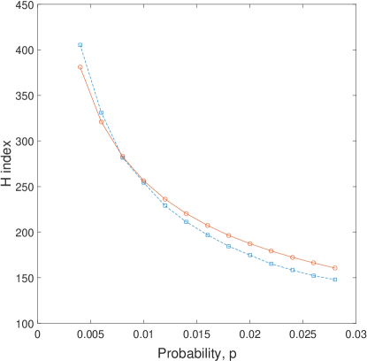
Figure 3: (a) Change of the $H$ index with the increase of the probability $p$ in ER random graphs $G_{ER}\left(1000,p\right)$ obtained using the formula (59) (empty circles and solid line) and using the function ’expm’ in Matlab (squares and broken line). (b) Change of the $H$ index with the increase of $m_{0}$ in BA random graphs $G_{BA}\left(1000,m_{0}\right)$ obtained using the formula (69) (empty circles and solid line) and using the function ’expm’ in Matlab (squares and broken line). All the calculations are the average of 100 random realizations.

It is easy to show that for a given value of $r$, $H\left(BA\right)>H\left(ER\right).$ That is, for the same network density the network having power-law degree distribution has larger value of the $H$ index than the analogous one with Poisson degree distribution. This result is somehow expected from the qualitative analysis of the eigenvalues distributions of these two classes of random networks. While the ER networks display a semicircle distribution of eigenvalues, the BA networks for small values of $r$ displays a triangular distribution peaked at $\lambda_{j}=0$. In other words, the nullity of the BA graphs is larger than that of the ER ones, and the concentration of eigenvalues close to zero is also larger for the BA networks than for the ER. Both characteristics give rise to larger values of the $H$ index in the BA networks. The question that arises here is what this difference implies from the structural point of view. We will analyze this question in the remaining part of this section.

We have already seen that the largest values of the $H$ index occurs in graphs having complete bipartite structures. Then, in order to understand the main structural differences giving rise to the larger $H$ index in BA networks than in ER ones we consider the existence of such subgraphs in both networks. In particular, we will consider the existence of complete bipartite subgraphs, known as bicliques, in both kind of networks. In the current work we will give only a qualitative explanation of this difference which will point to the direction of a further quantitative analysis. Let us start by the analysis of the BA networks. These networks are created from an initial seed of $n_{0}$ nodes connected randomly and independently according to the ER model. Then, at each stage of the evolution of the network, a new node is connected preferentially to $m_{0}\leq n_{0}$ nodes. The connection probability is proportional to the degree of the existing nodes. Because an ER network is uncorrelated the probability that the highest degree nodes are connected to each other is relatively low. Then, when a new node is added and connected to $m_{0}$ of the highest degree existing nodes there is a high probability that a biclique is formed. Such a process is continued as more nodes are added to the graph, resulting a large bicliques with high probability (see Figure 4). The creation of an ER network follows a completely different process in which pairs of nodes are connected randomly and independently, which does not generates any preferred subgraphs, thus not producing a large number of bicliques. This qualitative analysis explaining structurally the existence of networks with high values of the $H$ index will be very useful in the next section of this work where we will analyze real-world networks.

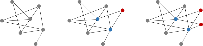
Figure 4: Illustration of the evolution of a graph under the BA model to sketch how bicliques are formed in such kind of networks. (a) Seed of $n_{0}=7$ nodes created with a Poissonian degree distribution to start the BA evolution process. (b) Given $m_{0}=2$ the new node (red one) is preferentially attached to those with the highest degree among the existing $n_{0}$ ones (marked in blue). (c) Second iteration of the process, which creates a biclique $K_{2,2}$ (red and blue nodes joined by dotted lines).

V Studies of real-world networks

V.1 Datasets

In this section we study a group of real-world networks representing a variety of social, environmental, technological, infrastructural and biological complex systems. A description of the networks and their main characteristics are given below.

Brain networks

• Neurons: Neuronal synaptic network of the nematode C. elegans. Included all data except muscle cells and using all synaptic connections Milo datasets ; Cat and macaque visual cortices: the brain networks of macaque visual cortex and cat cortex, after the modifications introduced by Sporn and Kï¿œtter Brain networks datasets .

Ecological networks

• Benguela: Marine ecosystem of Benguela off the southwest coast of South Africa Benguela ; Bridge Brook: Pelagic species from the largest of a set of 50 New York Adirondack lake food webs Bridge Brooks ; Canton Creek: Primarily invertebrates and algae in a tributary, surrounded by pasture, of the Taieri River in the South Island of New Zealand Canton ; Chesapeake Bay: The pelagic portion of an eastern U.S. estuary, with an emphasis on larger fishes Chesapeake ; Coachella: Wide range of highly aggregated taxa from the Coachella Valley desert in southern California Coachella ; El Verde: Insects, spiders, birds, reptiles and amphibians in a rainforest in Puerto Rico ElVerde ; Grassland: all vascular plants and all insects and trophic interactions found inside stems of plants collected from 24 sites distributed within England and Wales Grassland ; Little Rock: Pelagic and benthic species, particularly fishes, zooplankton, macroinvertebrates, and algae of the Little Rock Lake, Wisconsin, U.S. LittleRock ; Reef Small: Caribbean coral reef ecosystem from the Puerto Rico-Virgin Island shelf complex Reef Small ; Scotch Broom: Trophic interactions between the herbivores, parasitoids, predators and pathogens associated with broom, Cytisus scoparius, collected in Silwood Park, Berkshire, England, UK Scotch Broom ; Shelf: Marine ecosystem on the northeast US shelf Shelf ; Skipwith: Invertebrates in an English pond Skipwith ; St. Marks: Mostly macroinvertebrates, fishes, and birds associated with an estuarine seagrass community, Halodule wrightii, at St. Marks Refuge in Florida StMarks ; St. Martin: Birds and predators and arthropod prey of Anolis lizards on the island of St. Martin, which is located in the northern Lesser Antilles StMartin ; Stony Stream: Primarily invertebrates and algae in a tributary, surrounded by pasture, of the Taieri River in the South Island of New Zealand in native tussock habitat Stony ; Ythan_1: Mostly birds, fishes, invertebrates, and metazoan parasites in a Scottish Estuary Ythan1 ;Ythan_2: Reduced version of Ythan1 with no parasites Ythan2 .

• Termite: The networks of three-dimensional galleries in termite nests Termite Moulds ; Ant: The network of galleries created by ants Ants ; Dolphins: social network of frequent association between 62 bottlenose dolphins living in the waters off New Zealand Dolphins ;

Informational networks

• Centrality: Citation network of papers published in the field of Network Centrality centrality ; deNooy ; GD: Citation network of papers published in the Proceedings of Graph Drawing during the period 1994-2000 GD ; ODLIS: Vocabulary network of words related by their definitions in the Online Dictionary of Library and Information Science. Two words are connected if one is used in the definition of the other ODLIS ; Roget: Vocabulary network of words related by their definitions in Roget’s Thesaurus of English. Two words are connected if one is used in the definition of the other Roget ; Small World: Citation network of papers that cite S. Milgram’s 1967 Psychology Today paper or use Small World in title Batagelj Mrvar .

Biological networks

• Protein-protein interaction networks in: Kaposi sarcoma herpes virus (KSHV) KSHV ; P. falciparum (malaria parasite) malaria ; S. cerevisiae (yeast) PIN_yeast_1 ; PIN_yeast_2 ; A. fulgidus PIN_Afulgidus ; H. pylori PIN_Hpylori ; E. coli PIN_Ecoli and B. subtilis PIN_Bsubtilis .

• Trans_E.coli: Direct transcriptional regulation between operons in Escherichia coli MiloDatasets2 ; MiloDatasets3 ; Trans_sea_urchin: Developmental transcription network for sea urchin endomesoderm development. MiloDatasets2 ; Trans_yeast: Direct transcriptional regulation between genes in Saccaromyces cerevisae. Milo datasets ; MiloDatasets2 .

Social and economic networks

• Corporate: American corporate elite formed by the directors of the 625 largest corporations that reported the compositions of their boards selected from the Fortune 1000 in 1999 Corporate ; Geom: Collaboration network of scientists in the field of Computational Geometry Batagelj Mrvar ; Prison: Social network of inmates in prison who chose “What fellows on the tier are you closest friends with?” Prison ; Drugs: Social network of injecting drug users (IDUs) that have shared a needle in the last six months Moody ; Zachary: Social network of friendship between members of the Zachary karate club Zachary ; College: Social network among college students in a course about leadership. The students choose which three members they wanted to have in a committee College ; ColoSpring: The risk network of persons with HIV infection during its early epidemic phase in Colorado Spring, USA, using analysis of community wide HIV/AIDS contact tracing records (sexual and injecting drugs partners) from 1985-1999 ColoSpg ; Galesburg: Friendship ties among 31 physicians deNooy ; High_Tech: Friendship ties among the employees in a small high-tech computer firm which sells, installs, and maintain computer systems HighTech ; deNooy ; Saw Mills: Social communication network within a sawmill, where employees were asked to indicate the frequency with which they discussed work matters with each of their colleagues SawMill ; deNooy ;

Technological and infrastructural networks

• Electronic: Three electronic sequential logic circuits parsed from the ISCAS89 benchmark set, where nodes represent logic gates and flip-flop Milo datasets ; USAir97: Airport transportation network between airports in US in 1997 Batagelj Mrvar ; Internet: The internet at the Autonomous System (AS) level as of September 1997 and of April 1998 Internet ; Power Grid: The power grid network of the Western USA WattsStrogatz .

Software networks

• Collaboration networks associated with six different open-source software systems, which include collaboration graphs for three Object Oriented systems written in C++, and call graphs for three procedural systems written in C. The class collaboration graphs are from version 4.0 of the VTK visualization library; the CVS snapshot dated 4/3/2002 of Digital Material (DM), a library for atomistic simulation of materials; and version 1.0.2 of the AbiWord word processing program. The call graphs are from version 3.23.32 of the MySQL relational database system, and version 1.2.7 of the XMMS multimedia system. Details of the construction and/or origin of these networks are provided in Myers Myers Software .

V.2 Analysis of real-world networks

The sizes of the networks studied here range from 29 to 4,941 nodes. Then, in order to avoid any size influence, we normalize the $H$ index by dividing it by the number of nodes of the network. We will call $\hat{H}$ to the normalized index. The normalized index $\hat{H}$ ranges from about 0.14 to about 0.75 for the studied networks, indicating that real-world networks cover most of the values that this index can take (see 1). The scatterplot of the normalized nullity versus the normalized $H$ index for the 61 real-world networks studied here (plot not shown) reveals that although both indices follow the same trend, there are important differences among them. In particular, we can observe that there are 9 networks with zero nullity which display values of $\hat{H}$ ranging from about 0.14 (the lowest $\hat{H}$ index) to about 0.36 (ranked 25th in increasing order of $\hat{H}$ index).

Name	$n$	$H$	$EE$	$\eta$	$r$
Ants	74	30.998	2.64E+02	14	-0.102
Benguela	29	9.573	4.11E+06	0	0.021
BridgeBrook	75	56.018	9.20E+08	48	-0.668
Canton	108	40.333	3.12E+08	24	-0.226
CatCortex	52	12.636	8.95E+09	0	-0.044
Centrality_literature	118	42.976	2.44E+08	9	-0.202
Chesapeake	33	13.240	4.71E+02	3	-0.196
Coachella	30	10.984	7.61E+07	0	0.035
ColoSpg	324	182.077	1.15E+03	142	-0.295
CorporatePeople	1586	228.395	1.27E+10	0	0.268
Dolphins	62	20.845	2.06E+03	2	-0.044
Drugs	616	279.467	6.91E+07	131	-0.117
Electronic1	122	37.694	4.84E+02	0	-0.002
Electronic2	252	77.982	1.04E+03	8	-0.006
Electronic3	512	158.658	2.17E+03	24	-0.030
ElVerde	156	51.696	4.76E+13	5	-0.174
Galesburg	31	9.519	4.36E+02	1	-0.135
GD	249	90.440	1.60E+04	15	0.098
Geom	3621	1462.396	4.04E+12	537	0.168
Hi_tech	33	10.975	2.95E+03	1	-0.087
Internet1997	3015	2148.635	6.17E+13	1883	-0.229
Internet1998	3522	2473.122	1.42E+15	2158	-0.210
LittleRockA	181	117.772	5.32E+17	93	-0.234
MacaqueVisualCortex	32	9.665	1.26E+06	1	0.008
Neurons	280	69.083	1.31E+10	3	-0.069
ODLIS	2898	1131.046	1.54E+19	270	-0.173
PIN_Afulgidus	32	16.366	9.91E+01	12	-0.472
PIN_Bsubtilis	84	53.144	3.52E+02	46	-0.486
PIN_Ecoli	230	102.189	8.30E+06	57	-0.015
PIN_Hpyroli	710	397.649	4.60E+04	316	-0.243
PIN_KSHV	50	18.119	1.82E+03	2	-0.058
PIN_Malaria	229	83.377	2.25E+04	13	-0.083
PIN_Yeast	2224	1135.731	1.94E+08	754	-0.105
Power_grid	4941	1907.307	2.13E+04	593	0.003
PRISON	67	20.325	7.08E+02	0	0.103
ReefSmall	50	12.888	2.07E+10	0	-0.193
Roget	994	264.570	2.38E+05	2	0.174
Sawmill	36	12.307	2.57E+02	2	-0.071
ScotchBroom	154	103.975	2.46E+06	90	-0.311
Shelf	81	20.724	1.60E+18	2	-0.094
Skipwith	35	15.023	3.87E+09	7	-0.319
SmallWorld	233	115.730	1.27E+09	70	-0.303
College	32	8.049	5.36E+02	0	-0.119
Software_Abi	1035	575.133	1.65E+05	418	-0.086
Software_Digital	150	82.277	1.31E+03	63	-0.228
Software_Mysql	1480	648.971	2.70E+09	282	-0.083
Software_VTK	771	440.251	1.11E+05	324	-0.195
Software_XMMS	971	478.168	4.64E+04	294	-0.114
StMarks	48	13.607	1.43E+05	0	0.111
StMartin	44	14.438	2.78E+05	2	-0.153
Stony	112	41.359	7.23E+09	30	-0.222
Termite_1	507	206.581	1.92E+03	75	-0.046
Termite_2	260	116.912	7.32E+02	58	-0.150
Termite_3	268	100.975	1.89E+03	23	0.045
Trans_Ecoli	328	214.517	1.06E+04	184	-0.265
Trans_urchin	45	22.218	9.12E+02	13	-0.207
Transc_yeast	662	478.315	3.59E+04	440	-0.410
USAir97	332	142.765	8.08E+17	58	-0.208
Ythan1	134	58.374	1.86E+07	23	-0.263
Ythan2	92	41.326	7.07E+06	22	-0.322
Zackar	34	15.994	1.04E+03	10	-0.476

Table 1. Dataset of real-world networks studied in this paper, their size $n$, Gaussian Estrada index $H$, exponential Estrada index $EE,$ graph nullity $\eta$, and degree assortativity $r$.

The largest value of $\hat{H}$ corresponds to the food web of Bridge Brooks, which displays the second highest normalized nullity. It is followed by the transcription network of yeast (displaying the highest value of the normalized nullity) and the versions of Internet at Autonomous System (AS) of 1997 and 1998. The three networks display triangular eigenvalue distributions peaked at the zero eigenvalue which explains their large values of the $\hat{H}$ index. However, while the yeast transcription network and the Internet at AS have fat-tailed degree distributions, the Bridge Brooks food web displays a uniform one. Thus, the existence of large values of the $\hat{H}$ index is not tied up to the existence of fat-tailed degree distributions. Most of the networks (75.4%) have values of the $\hat{H}$ index below 0.5. That is, only 15 networks out of 61 have $\hat{H}\geq 0.5$. Among these 15 networks there are 4 of the 7 protein-protein interaction networks (PINs) studied and two of the three transcription networks studied. Thus, almost half of the networks with $\hat{H}\geq 0.5$ represent biological systems containing proteomic or transcriptomic information. The other transcription network studied has $\hat{H}\approx 0.494$ and the other 3 PINs have values of $\hat{H}$ ranging between 0.36 and 0.44. It is interesting to explore the main structural causes for these high values of the $\hat{H}$ index. In previous sections we have found that the main structural characteristic determining the high values of this index is the presence of bicliques, e.g. the highest value of $\hat{H}$ is obtained for complete bipartite graphs, also the BA networks display larger $\hat{H}$ index that the ER ones due to the presence of complete bipartite subgraphs created during the evolution of the preferential attachment mechanism. Consequently, we should expect that such kind of subgraphs appear in those real-world networks having the largest $\hat{H}$ index. In the case of the food web of Bridge Brook we have found a biclique consisting of two sets of nodes $V_{1}$ and $V_{2}$with cardinalities of 6 and 35 nodes, respectively. This subgraph represents a biclique $K_{6,35}$ which contains 55% of the total number of nodes in the network. There are also other smaller bicliques in this network, which together with the $K_{6,35}$ contribute to the large $\hat{H}$ value observed. In the cases of the yeast transcription network and the Internet at AS, the networks are characterized by having a few hubs connected to many nodes of degree one, then producing bicliques of the type $K_{1,n_{2}}.$ In general these findings can be understood on the basis of different mechanisms which give rise to the existence of bicliques in real-world networks. For instance, in some food webs there are top predators which compete for a group of preys. If for this group of species there are no prey-prey nor predator-predator trophic interactions, the corresponding subgraph is a biclique as the one observed for the Bridge Brook network previously considered. In the cases of transcription and PINs the bicliques can be formed as a consequence of lock-and-key kind of interaction. That is, a group of proteins (genes) can act as locks (activators) that physically interact with other proteins (activate other genes) acting as keys. Such kind of interactions is prone to produce relatively large bicliques in the structure of the networks resulting from them.

On the other hand, among the networks with $\hat{H}\leq 0.3$ we find the network of corporate directors, the three neuronal networks studied, i.e., macaque and cat visual cortex and the neuronal network of C. elegans, as well as some social networks and food webs. Also, the three electronic circuits studied here also display values of $\hat{H}$ index around 0.3. These networks are characterized by the lack of complete bipartite subgraphs and they may represent a variety of topologies difficult to be reproduced by a single mechanism.

Finally we would like to remark a few important characteristics of the Gaussian matrix function of a network that point out to the necessity of further studies of it for real-world networks and simple graphs in general. The first, is our observation that although networks with fat-tailed degree distribution may give rise to high values of the $\hat{H}$ index, it is not a necessary condition for a network to display such a characteristic. We have seen that networks with exponential and even uniform degree distributions display large values of the $\hat{H}$ index. Another structural parameter that could be related to the $\hat{H}$ index is the degree assortativity, i.e., the Pearson correlation coefficient of the degree-degree distribution of a network. We have explored such relation between the $\hat{H}$ index and the assortativity for the 61 networks studied here. We have found that the two parameters are negatively correlated. That is, high values of the $\hat{H}$ index in general implies that the networks are disassortative, i.e., there is a trend of high degree nodes to be connected to low degree ones. This is understandable on the basis of our findings that bicliques of the type $K_{1,n_{2}}$ plays a fundamental role in the value of the $\hat{H}$ index. However, the correlation is very weak and displays a Pearson correlation coefficient of -0.68. Thus, further explorations—both theoretical and computational—of the relation of the $\hat{H}$ index and other network parameters are necessary for a complete understanding of this index and its application in network theory.

VI Summary

Most of the works using matrix functions for studying graphs are concentrated on the use of the exponential and the resolvent of the adjacency matrix of the graph. Other functions such as the hyperbolic sine and cosine, and $\psi$-matrix functions have also been reported. All these matrix functions give more weight to the largest eigenvalue and the corresponding eigenvector of the adjacency matrix than to the rest of eigenvalues/eigenvectors. In many real-world networks, where the spectral gap is relatively large, this situation gives rise to discarding important structural information contained in the eigenvalues close to zero in the graph spectra. Here, we have studied a Gaussian matrix function which accounts for the information contained in the eigenvalues/eigenvectors close to zero in the graph spectra. We have shown that such information is related to the existence of important structural patterns in graphs which have remained unexplored when studying the structure of complex networks, such as the existence of relatively large complete bipartite subgraphs (bicliques). Such bicliques appear naturally in many real-world networks as well as in the Barabï¿œsi-Albert graphs and other networks with fat-tailed degree distributions. In this work we have concentrated in the theoretical characterization of the networks displaying the largest Gaussian Estrada index—an index characterizing the importance of eigenvalues close to zero. Other extensions to give more weight to other specific eigenvalues/eigenvectors of the adjacency matrix are under development. We hope this work will open new research interest in the study of matrix functions for the structural characterization of graphs.

References

- (1) N. J. Higham, Functions of Matrices: Theory and Computation. (Society for Industrial and Applied Mathematics, Philadelphia, PA, 2008).
- (2) E. Estrada, and D. J. Higham, “Network properties revealed through matrix functions,” SIAM Rev. 52, 696–714 (2010).
- (3) E. Estrada, and N. Hatano, “Communicability in complex networks,” Phys. Rev. E 77, 036111 (2008).
- (4) E. Estrada, “Characterization of the folding degree of proteins,” Bioinformatics 18, 697–704 (2002).
- (5) E. Estrada, and J.A. Rodrï¿œguez-Velï¿œzquez, “Subgraph centrality in complex networks,” Phys. Rev. E, 71, 056103 (2005).
- (6) E. Estrada, N. Hatano, and M. Benzi, “The physics of communicability in complex networks,” Phys. Rep. 514, 89–119 (2012).
- (7) L. Katz, “A new index derived from sociometric data analysis,” Psychometrika 18, 39–43 (1953).
- (8) J.A. de la Peï¿œa, I. Gutman, and J. Rada, “Estimating the Estrada index,” Lin. Algebra Appl. 427, 70–76 (2007).
- (9) H. Deng, S. Radenković, and I. Gutman, “The Estrada index,” in Applications of Graph Spectra, edited by D. Cvetković, I. Gutman, (Math. Inst, Belgrade, 2009), pp. 123–140.
- (10) I. Gutman, H. Deng, and S. Radenković, “The Estrada index: an updated survey,” in Selected Topics on Applications of Graph Spectra, edited by D. Cvetković, I. Gutman, (Math. Inst, Belgrade, 2011), pp. 155–174.
- (11) J. Wu, M. Barahona, Y-J. Tan, and H-Z. Deng. “Robustness of regular ring lattices based on natural connectivity,” Int. J. Syst. Sci. 42, 1085-1092, 2011.
- (12) J. Wu, H.-Z. Deng, Y.-J. Tan, and D.-Z. Zhu, “Vulnerability of complex networks under intentional attack with incomplete information,” J. Phys. A: Math. Theor. 40, 2665 (2007).
- (13) M. Benzi, E. Estrada, and C. Klymko, “Ranking hubs and authorities using matrix functions,” Lin. Algebra Appl., 438, 2447-2474(2013).
- (14) M. Benzi, and C. Klymko, “On the limiting behavior of parameter-dependent network centrality measures,” SIAM J. Matrix Anal. Appl. 36, 686-706 (2015).
- (15) F. Arrigo, and M. Benzi, “Updating and downdating techniques for optimizing network communicability,” SIAM J. Sci. Comp. 38, B25-B49 (2016).
- (16) E. Estrada, “Graphs and Networks,” in Mathematical Tools for Physicists, edited by M. Grinfeld, (John Wiley & Sons, 2014), pp. 111–157
- (17) E. Estrada, The Structure of Complex Networks. Theory and Applications. (Oxford University Press, 2011).
- (18) L. F. Costa, O. N. Oliveira Jr, and G. Travieso, et al. “Analyzing and modeling real-world phenomena with complex networks: a survey of applications,” Adv. Phys. 60, 329–412 (2011).
- (19) E. Estrada, “Generalized walks-based centrality measures for complex biological networks,” J. Theor. Biol. 263,556–565 ( 2010).
- (20) W. Kutzelnigg, “What I like about Hï¿œckel theory,” J. Comput. Chem. 28, 25–34 (2007).
- (21) K. Yates, Hï¿œckel molecular orbital theory. (Elsevier, 2012).
- (22) B. Borovićanin, and I. Gutman, “Graph nullity,” in Selected Topics on Applications of Graph Spectra, edited by D. Cvetković, I. Gutman, (Math. Inst, Belgrade, 2011), pp. 155–174.
- (23) K. Fukui, T. Yonezawa, H. Shingu, “A Molecular Orbital Theory of Reactivity in Aromatic Hydrocarbons,” J. Chem. Phys. 20, 722–725 (1952).
- (24) K. Fukui, “The role of frontier orbitals in chemical reactions (Nobel Lecture),” Angewandte Chemie Int. Ed. Engl. 21, 801-809 (1982).
- (25) I. Fleming, Frontier Orbitals and Organic Chemical Reactions. (London: Wiley, 1978), pp.ï¿œ29–109.
- (26) E. Estrada, D. J. Higham, and N. Hatano, “Communicability betweenness in complex networks,” Physica A 388, 764–774 (2009)
- (27) J. E. Hirsch, and J. R. Schrieffer, “Dynamic correlation functions in quantum systems: A Monte Carlo algorithm,” Phys. Rev. B 28, 5353–5356 (1983).
- (28) E. R. Gagliano and C. A. Balseiro, “Dynamic correlation functions in quantum many-body systems at zero temperature,” Phys. Rev. B 38, 11766–11773 (1988).
- (29) J. E. Barrios-Vargas and G. G. Naumis, “Doped graphene: the interplay between localization and frustration due to the underlying triangular symmetry,” J. Phys.: Condens. Matter 23, 375501 (2011).
- (30) E. Estrada, and M. Benzi, “Atomic displacements due to spin-spin repulsion in conjugated alternant hydrocarbons,” Chem. Phys. Lett. 568-569, 184–189 (2013).
- (31) M. Benzi, P. Boito, “Quadrature rule-based bounds for functions of adjacency matrices,” Lin. Algebra Appl. 433, 637–652 (2010).
- (32) M. Benzi, and G. H. Golub, “Bounds for the entries of matrix functions with application to preconditioning,” BIT 39, 417–438 (1999).
- (33) M. Benzi, and P. Boito, “Quadrature rule-based bounds for functions of adjacency matrices,” Lin. Algebra Appl. 433, 637–652 (2010).
- (34) G. H. Golub, and G. Meurant, Matrices, Moments and Quadrature with Applications. (Princeton University Press, Princeton, NJ 2010).
- (35) L. Collatz, and U. Sinogowitz, “Spektren Endlicher Grafen,” Abh. Math. Sem. Univ. Hamburg 21, 63–77 (1957).
- (36) P. Erdős, A. Rï¿œnyi, “On Random Graphs,” I, Publicationes Mathematicae 6, 290–297 (1959).
- (37) E. N. Gilbert, “Random Graphs,” Annals Math. Stat. 30, 1141–1144 (1959).
- (38) A.-L. Barabï¿œsi, R. Albert, “Emergence of scaling in random networks,” Science 286, 509–512 (1999).
- (39) E. Wigner, “Characteristic vectors of bordered matrices with infinite dimensions,” Ann. of Math. 62, 548–564 (1955).
- (40) M. Krivelevich, and B. Sudakov, “The largest eigenvalue of sparse random graphs,” Combin. Probab. Comput. 12, 61–72 (2003).
- (41) R. Milo, S. Shen–Orr, S. Itzkovitz, et al., “Network motifs: simple building blocks of complex networks,” Science 298, 824–827 (2002).
- (42) C. R. Myers, “Software systems as complex networks: Structure, function, and evolvability of software collaboration graphs,” Phys. Rev. E 68, 046116 (2003).
- (43) J. L. Lockwood, R. D. Powell, M. P. Nott, and S. L. Pimm, “Assembling ecological communities in time and space,” Oikos 549-553 (1997).
- (44) A. G. Rossberg, H. Matsuda, T. Amemiya, and K. Itoh, “Food webs: experts consuming families of experts,” J. Theor. Biol. 241, 552-563 (2006).
- (45) O. Sporns, and R. Kï¿œtter. “Motifs in brain networks,” PLoS Biology 2, e369 (2004).
- (46) P. Yodzis, “Diffuse effects in food webs,” Ecology 81, 261-266 (2000).
- (47) G. A. Polis, “Complex trophic interactions in deserts: an empirical critique of food-web theory,” Am. Nat. 138, 123-155 (1991).
- (48) C. Townsend, R. M. Thompson, and A. R. McIntosh, et al. “Disturbance, resource supply, and food-web architecture in streams,” Ecol. Lett. 1, 200 (1998).
- (49) R. R. Christian, and J. J. Luczkovich, “Organizing and understanding a winter’s seagrass foodweb network through effective trophic levels,” Ecol. Model. 117, 99-124 (1999).
- (50) P. H. Warren,“Spatial and temporal variation in the structure of a fresh-water food web,” Oikos 55, 299-311 (1989).
- (51) R. B. Waide, and W. B. Reagan, (Eds.) The Food Web of a Tropical Rainforest. (University Chicago Press, Chicago, 1996).
- (52) N. D. Martinez, B. A. Hawkins, H. A. Dawah, and B. P. Feifarek, “Effects of sampling efforts on characterization of food web structure,” Ecology 80, 1044–1055 (1999).
- (53) K. Havens, “Scale and structure in natural food webs,” Science 257, 1107-1109 (1992).
- (54) S. Opitz, “Trophic Interactions in Caribbean coral reefs,” ICLARM Tech. Rep. 43, Manila, Philippines, (1996).
- (55) J. Memmott, N. D. Martinez, and J. E. Cohen, “Predators, parasites and pathogens: species richness, trophic generality, and body sizes in a natural food web,” J. Animal Ecol. 69, 1-15 (2000).
- (56) J. Link, “Does food web theory work for marine ecosystems?,” Mar. Ecol. Prog. Ser. 230, 1-9 (2002).
- (57) P. Yodzis, “Local trophodynamics and the interaction of marine mammals and fisheries in the Benguela ecosystem,” J. Anim. Ecol. 67, 635-658 (1998).
- (58) L. Goldwasser, and J. A. Roughgarden, “Construction and analysis of a large Caribbean food web,” Ecology 74, 1216-1233 (1993).
- (59) N. D. Martinez, “Artifacts or attributes? Effects of resolution on the Little Rock Lake food web,” Ecol. Monogr. 61, 367-392 (1991).
- (60) D. Baird, and R. E. Ulanowicz, “The seasonal dynamics of the. Chesapeake Bay ecosystem,” Ecol. Mon. 59, 329-364 (1989).
- (61) M. Huxman, S. Beany, and D. Raffaelli, “Do parasites reduce the chances of triangulation in a real food web?,” Oikos 76, 284-300 (1996).
- (62) S. J. Hall, and D. Rafaelli, “Food-web patterns - lessons from a species-rich web,” J. Anim. Ecol. 60, 823–842 (1991).
- (63) N. P. Hummon, P. Doreian, and L. C. Freeman, “Analyzing the structure of the centrality-productivity literature created between 1948 and 1979,” Know.-Creat. Diffus. Util. 11, 459-480 (1990).
- (64) W. de Nooy, A. Mrvar, and V. Batagelj, Exploratory Social Network Analysis with Pajek, Cambridge University Press, Cambridge (2005).
- (65) V. Batagelj, and A. Mrvar, “Graph Drawing Contest 2001,” http://vlado.fmf.uni-lj.si/pub/GD/GD01.htm. (2001).
- (66) ”ODLIS: Online Dictionary of Library and Information Science,” http://vax.wcsu.edu/library/odlis.html. (2002).
- (67) Roget´s Thesaurus of English Words and Phrases, Project Gutenberg. http://gutenberg.net/etext/22 (2002).
- (68) V. Batagelj, and A. Mrvar, Pajek datasets. Available at: http://vlado.fmf.uni-lj.si/pub/networks/data/ (2006).
- (69) P. Uetz, Y.-A. Dong, and Ch. Zeretzke, et al., “Herpesviral protein networks and their interaction with the human proteome,” Science 311, 239-242 (2006).
- (70) D. LaCount, M. Vignali, and R. Chettier, et al. “A protein interaction network of the malaria parasite Plasmodium falciparum,” Nature 438, 103–107 (2005).
- (71) D. Bu, Y. Zhao, and L. Cai, et al. “Topological structure analysis of the protein-protein interaction network in budding yeast,” Nucleic Acids Res. 31, 2443-2450 (2003).
- (72) C. von Mering, R. Krause, and B. Snel, et al. “Comparative assessment of large-scale data sets of protein-protein interactions,” Nature 417, 399-403 (2002).
- (73) M. Motz, I. Kober, and C. Girardot, et al. “Elucidation of an Archaeal Replication Protein Network to Generate Enhanced PCR Enzymes,” J. Biol. Chem. 277, 16179–16188 (2002).
- (74) C. Y. Lin, C. L. Chen, C. S. Cho, et al. “hp-DPI: Helicobacter pylori database of protein interactomes. A combined experimental and inferring interactions,” Bioinformatics 21, 1288–1290 (2005).
- (75) G. Bultland, J. M. Peregrï¿œn-Alvarez, and J. Li, et al. “Interaction network containing conserved and essential protein complexes in Escherichia coli,” Nature 433, 531-537 (2005).
- (76) P. Noirot, and N. F. Noirot-Gross, “Protein interaction networks in bacteria,” Curr. Op. Microb. 7, 505–512 (2004).
- (77) R. Milo, S. Itzkovitz, and N. Kashtan, et al. “Superfamilies of evolved and designed networks,” Science 303, 1538-1542 (2004).
- (78) S. Shen-Orr, R. Milo, S. Mangan, and U. Alon, “Network motifs in the transcriptional regulation network of Escherichia coli,” Nature Gen. 31, 64-68 (2002).
- (79) G. F. Davis, M. Yoo, and W. E. Baker, “The Small World of the American Corporate Elite, 1982-2001,” Strategic Organization 1, 301-326 (2003).
- (80) D. MacRae, “Direct factor analysis of sociometric data,” Sociometry 23, 360-371 (1960).
- (81) D., Lusseau, “The emergent properties of a dolphin social network,” Proc. R. Soc. Lond. B (Suppl.) 270, 186-188 (2003).
- (82) J. Moody, Data for this project was provided in part by NIH grants DA12831 and HD41877, those interested in obtaining a copy of these data should contact James Moody (moody.77@sociology.osu.edu), (2001).
- (83) W. Zachary, “An information flow model for conflict and fission in small groups,” J. Anthropol. Res. 33, 452-473 (1977).
- (84) L. D. Zeleny, “Adaptation of research findings in social leadership to college classroom procedures,” Sociometry 13, 314-328 (1950).
- (85) J. J. Potterat, L. Philips-Plummer, and S. Q. Muth, et al. “Risk network structure in the early epidemic phase of HIV transmission in Colorado Springs,” Sex. Transm. Infect. 78, i159-i163 (2002).
- (86) D. Krackhardt, “The ties that torture: Simmelian tie analysis in organizations” Res. Sociol. Org. 16, 183-210 (1999).
- (87) J. H. Michael, and J. G. Massey, “Modeling the communication network in a sawmill” Forest Prod. J. 47, 25-30 (1997).
- (88) M. Faloutsos, P. Faloutsos, and C. Faloutsos, “On power-law relationships of the internet topology” Comp. Comm. Rev. 29, 251-262 (1999).
- (89) D. J. Watts, and S. H. Strogatz, “Collective dynamics of small-world networks” Nature 393, 440-442 (1998).
- (90) A. Perna, S. Valverde, and J. Gautrais, et al. “Topological efficiency in the three-dimensional gallery networks of termite nests,” Physica A 387, 6235-6244 (2008).
- (91) J. Buhl, J. Gautrais, and R. V. Solï¿œ, et al. “Efficiency and robustness in ant networks of galleries,” Eur. Phys. J. B 42, 123-129 (2004).