Statistical discrete geometry

Abstract

Following our earlier work key-4.3 , we construct statistical discrete geometry by applying statistical mechanics to discrete (Regge) gravity. We propose a coarse-graining method for discrete geometry under the assumptions of atomism and background independence. To maintain these assumptions, we propose restrictions to the theory by introducing cut-offs, both in ultraviolet and infrared regime. Having a well-defined statistical picture of discrete Regge geometry, we take the infinite degrees of freedom (large $n$) limit. We argue that the correct limit consistent with the restrictions and the background independence concept is not the continuum limit of statistical mechanics, but the thermodynamical limit.

I Introduction

Attempts to understand the thermodynamical aspect of general relativity (GR) have already been studied through the thermodynamics of black holes key-1.1 ; key-1.2 ; key-1.3 ; key-8.5 . The first step to understand this problem is the discovery of the four laws of black hole mechanics, which resembles the laws of thermodynamics key-1.4 . According to the laws, black hole could emit Hawking radiation, due to the quantum effect of the infalling particles near the black hole’s horizon key-1.5 ; key-1.6 . As a consequence of the radiation, black holes must have temperature and entropy key-1.5 ; key-1.6 ; key-1.7 ; key-1.8 . The entropy should be a result of the existence of microstates of the black hole, which is not believed to exist before, due to the no-hair theorem key-1.9 ; key-1.10 ; key-1.11 . Loop quantum gravity (LQG) provides an explanation to the origin of Bekenstein-Hawking entropy from finite microstates-counting of the black hole key-1.1 ; key-1.2 . The latest results regarding the entropy of black hole from LQG are presented key-8.5 ; key-1.12 .

Attempts to quantize gravity have also developed, with canonical loop quantum gravity as one of these theories key-3.1 ; key-3.2 ; key-3.30 ; key-3.31 ; key-3.38 . The successful theory of quantum gravity should give a ’correct’ classical theory, -general relativity, in an appropriate limit key-8.1 ; key-1.13 ; key-1.14 . In loop quantum gravity, there are two parameters which can be adjusted to obtain this limit: the spin-number $j,$ which describes the size of the quanta of space, and the number of quanta $n,$ which describes the degrees of freedom in the theory. General relativity is expected to be obtained by taking the classical limit: the limit of large number of degrees of freedom and spins, $n,j\rightarrow\infty$; while the mesoscopic, or the semi-classical limit is obtained by taking only the spin number $j$ to be large, $j\rightarrow\infty$ key-8.1 ; key-1.13 ; key-1.14 . Tullio Regge have shown that discrete gravity will coincide with GR in the classical limit, at the level of the action, when the discrete manifold converge to Riemannian manifold key-3.19 ; key-3.23 . Moreover, Roberts have shown that the $6j$-symbol, which is used to describe the transition amplitude in canonical LQG key-3.31 ; key-3.20 , in the large-$j$ limit can be written as some functions, such that the transition amplitude of LQG coincides with the partition function of Regge discrete geometry key-7.21 . Attempts to obtain the continuum and semi-classical limit have already been studied key-8.1 ; key-7.15 ; key-1.15 ; key-1.16 , with the latest result is reported elsewhere key-1.13 .

This work is particularly more focused on the large $n$ limit. To handle a system with large degrees of freedom, it is convenient to use statistical mechanics as a coarse-graining tool. On the other hand, thermodynamics can also be explained from statistical mechanics point of view, as an ’effective’ theory emerging from the large degrees of freedom limit. Therefore, by using the language of statistical mechanics, the two distinct problems of gravity, namely, its thermodynamical aspects and the correct classical limit of quantum gravity, appear to be related to each other.

In this article, we construct statistical discrete geometry by applying statistical mechanics formulation to discrete (Regge) geometry. Our approach is simple: by taking the foliation of spacetime (compact space foliation in the beginning, then the extension to a non-compact case is possible) as our system, dividing it into several partitions, similar with many-body problem in classical mechanics, and then characterizing the whole system using fewer partitions, coarser degrees of freedom. We propose a coarse-graining procedure for discrete geometry using the lengths, areas, and volumes of the space as the variables to be taken the coarser, average value.

Two basic philosophical assumptions are taken in this work. These assumptions are fundamental in non-perturbative quantum gravity approach key-3.1 ; key-3.2 ; key-3.31 . First, is the atomism philosophy, which is the mainstream point of view adopted by physics in this century key-12 ; key-13 ; it assumes that every existing physical entities must be countable, which could be a humble way to treat infinities. Second, is the background independence concept key-3.2 ; key-3.34 ; key-3.35 , a point of view shared by many conservative quantum gravity theories, such as LQG, causal dynamical triangulation, and others. Loosely speaking, it assumes that the atoms of space do not need to live in another ’background’ space, so that we could localize these atoms. In other words, these atoms of space are the space, and we should not assume any other ’background stage’ for them.

To maintain the atomism philosophy, we propose two restrictions in our procedure by introducing cut-offs for the degrees of freedom, both in ultraviolet and infrared regions. In discrete geometry, these cut-offs truncate the theory with infinite degrees of freedom to a theory with finite degrees of freedom. As a direct consequence to these restriction, we obtain bounds on informational entropy, with consistent physical interpretations in the classical case.

A clear, well-defined procedure of a coarse-graining method will provide a first step to understand the problem mentioned in the beginning: the thermodynamical properties of general relativity and the correct classical limit of quantum gravity. In the last chapter of this work, we discuss the possibility to obtain the classical ’continuum’ limit of the kinematical LQG. Using the inverse method of coarse-graining called as refinement, and taking the limit of infinite degrees of freedom, we argue that the correct limit consistent with our two basic philosophical assumptions is not the continuum limit of statistical mechanics, but the thermodynamical limit. If this thermodynamical limit exist, theoretically, we could obtain the equation of states of classical gravity from (Regge) discrete geometry for the classical case.

The article contains four sections. In Section II, we propose a clear, well-defined coarse-graining procedure for any arbitrary classical system, and introduce two types of restriction to finitize the informational entropy. In Section III, we apply our coarse-graining procedure to discrete geometry, say, a set of connected simplices. A new results obtained in this chapter is the proposal of well-defined coarse-graining method and statistical discrete geometry formulation. The last section is the conclusion, where we give sketches about the generalization to the non-compact space case. We argue that the correct limit which will bring us to classical general relativity is not the ’continuum’ limit, but the thermodynamical limit of the statistical mechanics.

II Classical coarse-graining proposal

II.1 Definition of coarse-graining

In this section, we propose a precise definition of coarse-graining in the classical framework. It is defined as a procedure containing two main steps: reducing the degrees of freedom away to obtain reduced-microstates and then, taking the average state of all these possible reduced-microstates. A specific example is used to help to clarify the understanding. Suppose we have a classical system with two degrees of freedom. Let the degrees of freedom be represented by the energy of each partition $\left\{E_{1},E_{2}\right\}$, and let the coarse-graining procedure be defined as a way to represent this system using a single degrees of freedom.

II.1.1 Center-of-mass variables

Our system is characterized by variables $\left\{E_{1},E_{2}\right\}$, with $E_{1}$ and $E_{2}$ represent the energy of the first and second partitions, respectively. Suppose there exists a canonical ’transformation’ such that:

$$E_{\pm} = E_{1}\pm E_{2},$$ (1)

so that we have a new canonical variables $\left\{E_{+},E_{-}\right\}$, usually called as the center-of-mass variables. Each individual variable describes different thing: $\left\{E_{1},E_{2}\right\}$ describe the energy of each partition, while $\left\{E_{+},E_{-}\right\}$ describe the total energy of the system, and the energy difference between these two partitions. Nevertheless, both $\left\{E_{1},E_{2}\right\}$ and $\left\{E_{+},E_{-}\right\}$ describe the same system and have same amount of informations.

The next step is to treat this binary system as a single system, described by a single degree of freedom. This can be done naturally by taking only $E_{+}$ and neglecting the information of $E_{-}$. But having only $E_{+},$ the correct values of $\left\{E_{1},E_{2}\right\}$ can not be obtained, because there are no enough informations. With the correct $E_{-}$ unknown, then we obtain a set $\gamma$ representing $E_{+,}$ with all possible values of $E_{-}$.

II.1.2 Microstates, macrostate, sample space, and classical coarse-graining

In this subsection, we define new terminologies, which is slightly different with the usual statistical mechanics terminologies. Let $\mathbb{\gamma}$ be the physical configuration space. Let any point $\left\{E_{1}^{\left(j\right)},E_{2}^{\left(j\right)}\right\}$ or $\left\{E_{+}^{\left(j\right)},E_{-}^{\left(j\right)}\right\}$ element of $\mathbb{\gamma}$ be the $j^{th}$-microstates. Then we define the (total) energy of the microstate as $E_{1}^{\left(j\right)}+E_{2}^{\left(j\right)},$ which is exactly $E_{+}^{\left(j\right)}.$ For the discrete case, the microstate is $\left\{E_{1}^{\left(j\right)},E_{2}^{\left(j\right)}\right\}$ or $\left\{E_{+}^{\left(j\right)},E_{-}^{\left(j\right)}\right\},$ an element of a discrete set $\mathbb{\gamma}$ and $j\in\mathbb{Z},$ while for the continuous case, it is $\left\{E_{1}\left(x_{1}\right),E_{2}\left(x_{2}\right)\right\}$ or $\left\{E_{+}\left(x_{1},x_{2}\right),E_{-}\left(x_{1},x_{2}\right)\right\},$ an element of continuous set $\mathbb{\gamma}$ and $x_{1},x_{2}\in\mathbb{R}.$ Let $\left\{E_{1},E_{2}\right\}$ or $\left\{E_{+},E_{-}\right\}$ be the correct microstates and $E_{1}+E_{2}=E_{+}$ as the ’correct’ total energy.

Finally, we define the reduced $j^{th}$-microstate as $E_{+}^{\left(j\right)}$ and the correct reduced microstate as the ’correct’ total energy $E_{+}$. Our macrostate is the average over all possible reduced-microstates, under a probability distribution / weight $p_{j}$ for the discrete case, or a distribution function $p\left(\mathbf{x}\right)$ for the continuous case:

$$\overline{E} = \sum_{j}p_{j}E_{+}^{\left(j\right)},\qquad\textrm{(discrete case),}$$ (2)

$$\overline{E} = \intop_{\gamma}d\mathbf{x}\;p\left(\mathbf{x}\right)E_{+}\left(\mathbf{x}\right),\qquad\textrm{(continuous case),}$$ (3)

with $\mathbf{x}=\left(x_{1},x_{2}\right)$ is the measure on $\gamma$. The sample space $\mathbb{X}$ is the space of all possible microstates, which in this case, is $\gamma$. We define the macrostate $\bar{E}$ as our coarse-grained variable, the microstates as the fine-grained variables, and the procedure to obtain the macrostate as coarse-graining.

II.2 Restrictions

II.2.1 Distribution function and informational entropy

A specific probability distribution $p_{i}$ gives the probability for a specific microstate $i$ to occur. It defines a related entropy for the system. The definition of entropy we use in our work is the informational entropy or Shannon entropy, defined mathematically as key-2.2 :

$$S=-\sum_{i}p_{i}\ln p_{i}.$$ (4)

Moreover, we will use the generalization of Shannon entropy, the differential entropy key-2.3 :

$$S=-\intop_{0}^{\infty}\mathbf{dx}\>p\left(\mathbf{x}\right)\ln p\left(\mathbf{x}\right),$$ (5)

for a given continuous probability density $p\left(\mathbf{x}\right)\in C^{m}\left[\mathbb{R}^{n}\right]$, which is just the continuous version of Shannon entropy.

The informational entropy is the amount of lack-of-information of the coarse-grained state, with respect to the fine-grained state. See an analog-example in FIG. 1.

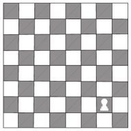
Figure 1: A nice analogy to help in understanding the informational entropy is by using a chess-board game. Suppose we want to know the location of the white pawn on the board. To know this, we need to ask questions such that the answers are only ’yes’ or ’no’. We can start by asking with: ’Is the pawn located at the half-left of the board?’, which will follow with the answer ’no’. We can repeat such question until we arrive at the right square. At this point, our information about the position of the pawn is already complete, and the entropy of the system is zero, since there is no lack-of-information in a ’completely-known’ system with maximal certainty.

We adapt the analogy to our microstates. The chess-board will be the sample space $\mathbb{X}$: the space of all possible microstates which correspond to a specific macrostate $\bar{E}$. Our ’correct’ microstate is a single point on the sample space $\mathbb{X}$, which is the location of the pawn in the example in FIG. 1. To arrive at this correct microstate, we need to ask question: ’Is the correct microstate located at some region $\mathbb{X}^{\prime}\subset\mathbb{X}$?’. If we could answer all the questions with binary answers (i.e., with ’yes / no’ answer) until we arrive to the correct microstate, then we know completely the information about the fine-grained state. This is the same as having the Dirac-delta distribution as a distribution function:

$$p\left(\mathbf{x}\right)=\delta\left(\overline{\mathbf{x}}-\mathbf{x}\right),$$ (6)

satisfying:

$$\intop_{0}^{\infty}\mathbf{dx}\>\delta\left(\overline{\mathbf{x}}-\mathbf{x}\right)f(\mathbf{x})=f(\overline{\mathbf{x}}),\quad\forall f,$$

with the specification $f(\overline{\mathbf{x}})=0$ if $\overline{\mathbf{x}}$ is not in the support of $f$. The distribution $\delta\left(\overline{\mathbf{x}}-\mathbf{x}\right)$ is normalized to unity:

$$\intop_{0}^{\infty}\mathbf{dx}\>\delta\left(\overline{\mathbf{x}}-\mathbf{x}\right)=1.$$

The corresponding informational entropy of a completely-known system should be zero. Obviously, the distribution function of a completely-known state should be the Dirac-delta function, since it points directly to a single microstate parametrized by $\overline{\mathbf{x}}$. By this reasoning, we expect the differential entropy of the Dirac-delta function is zero, but inserting (6) to (5) gives:

$$S=-\intop_{0}^{\infty}\mathbf{dx}\>\delta\left(\overline{\mathbf{x}}-\mathbf{x}\right)\ln\delta\left(\overline{\mathbf{x}}-\mathbf{x}\right) = -\infty.$$ (7)

This divergence comes from the fact that we have an infinitesimally small scale, which in physical term is known as the ultraviolet divergence key-2.4 .

II.2.2 Restrictions and bounds on entropy

In order to maintain the atomism philosophy as our starting point, we need to give restrictions to the sample space, and this results to the finiteness of the informational entropy key-2.5 .

Lower bound entropy

A continuous system, either finite or infinite, contains infinite amount of informations, which means it could have an infinite and/or arbitrarily small entropy. According to the atomism philosophy, it is necessary to have a finite amount of informations given a finite system, so that we only need to provide finite informations to know exactly the ’correct’ microstate of the system. Intuitively, we would like to have the entropy of the Dirac-delta function to be zero, since it points-out a single point on the sample space, which means we know completely the informations of the correct microstate. But from the calculation carried in the previous section, the differential entropy of the Dirac-delta function is $-\infty$. This is a consequence of allowing an infinitesimally-small scale in the theory, which leads to the UV-divergence. Therefore, to prevent UV-divergency, we consider the discrete version of the Dirac-delta, the Kronecker-delta, which is defined as:

$$\delta_{ij}\left\{\begin{array}[]{c}=0,\quad i\neq j\\ =1,\quad i=j\end{array}\right.,$$

normalized to unity:

$$\sum_{i=0}^{\infty}\delta_{ij}=1.$$

Adapting to our case, let the index $i$ runs from zero to any number (it can be extended to infinity), and let the index $j$ denotes our correct microstate. Obviously, the Kronecker-delta is the probability distribution of a completely-known system for the discrete version. We call the system in such condition as a ’pure state’, following the statistical quantum mechanics terminology. The Shannon entropy of this pure state is, by (4):

$$S_{\Delta}=-\sum_{i}^{\infty}\delta_{ij}\ln\delta_{ij}=0.$$

Therefore, in order to have a well-defined entropy for a pure state which is consistent with the physical interpretation, namely, the completely-known system, we need to give a restriction to the sample space $\mathbb{X}$:

Restriction 1 (Strong): The sample space must be discrete, in order to have a well-defined minimum entropy for a completely-known system with maximal certainty.

This means the possible microstates must be countable. The physical consequence of our first restriction is that all the corresponding physical properties (the ’observables’ in quantum mechanics term) must have discrete values. This statement, for our case, is equivalent with the statement: the spacing of the energy level can not be infinitesimally-small, there should exist an ultraviolet cut-off which prevent the energy levels to be arbitrarily small. This is exactly the expectation we have from the quantum theory.

Since the Shannon entropy (4) is definite positive, using the first restriction, we could define the lower bound of the informational entropy:

$$S_{\textrm{min}}=0,$$

which comes from the Kronecker-delta probability distribution, describing a completely-known state. This is in analog with the von-Neumann entropy bound on the pure state in quantum mechanics key-2.6 .

Upper-bound entropy

The completely-known ’pure’ state is an ideal condition where we know completely, without any uncertainty, all the informations of the correct microstate describing the system. This, sometimes, is an excessive requirement. In general, it is more frequent to have a state with an incomplete and uncertain information, a coarse-grained state. The probability distribution of this state could vary, from the normal to the homogeneous distribution.

Suppose we already obtain a specific probability distribution for the system, then we can ask questions: ’How much information we already know about the state? How certain is our knowledge about the state? How much information we need to provide to know the correct microstate?’ The answer to these questions depends on how much entropy we have when we obtain least information (maximal uncertainty) about the correct microstate.

Let us consider a state where we have no certainty in information about the correct microstate. Obviously, the probability distribution of such state should be a homogeneous distribution:

$$p_{i}=c,$$ (8)

with $c$ is a constant, and is normalized to unity:

$$\sum_{i}^{W}p_{i}=Wc=1,\qquad c=\frac{1}{W}.$$

In general, the discrete sample-space $\mathbb{X}$ is characterized by the index $i$ running from $0$ to $\infty,$ by the first restriction. If we extend the number of possible microstates $W$ to infinity, $c$ will go to zero. As a consequence, for an infinite, countable sample space, the ’upper bound’ of the entropy is $\infty$. Therefore, to obtain the correct microstate for such sample space, we need to provide an infinite amount of informations. This is not favourable, since the total amount of informations in the universe should be finite key-2.7 . It is necessary to add another restriction.

Restriction 2 (Weak): The sample space must be discrete and finite, in order to have a well-defined maximal entropy for a completely-unknown state with maximal uncertainty.

It means the number of possible microstates must be finite, besides being countable:

$$W<\infty.$$

The physical implication of the second restriction is that all the properties we want to take average, i.e., the properties of microstates $\left\{E_{1},E_{2}\right\}$ and $\left\{E_{+},E_{-}\right\}$ can not be infinitely large.

With the first and second restrictions, we can obtain the entropy for the homogeneous probability distribution:

$$S_{\Delta}=-\sum_{i=0}^{W}c\ln c=-\ln\frac{1}{W}=\ln W,$$ (9)

which gives Boltzmann definition of entropy key-2.8 : “the logarithm of number of all possible microstates”. This gives an upper bound on the entropy:

$$S_{\textrm{max}}=\ln W.$$

In conclusion, with first and second restrictions, we have a well-defined entropy for any probability distribution, within the range:

$$S_{\textrm{min}}\leq S\leq S_{\textrm{max}},$$ (10)

with $S_{\textrm{min}}=0$ and $S_{\textrm{max}}$ is the entropy of a completely ’ordered’ (completely-known) and completely random (completely-unknown) system, respectively.

II.3 General ensemble case

The example we used in the previous section is the microcanonical case. The correct microstate is $\left\{E_{1},E_{2}\right\}$, and the total energy of the correct microstate is $E_{+}=E_{1}+E_{2},$ which is also the correct reduced microstate. The microcanonical case is defined by the microcanonical constraint; this constraint need to be satisfied by any generic microstates:

$$E_{+}^{\left(j\right)}=E_{1}^{\left(j\right)}+E_{2}^{\left(j\right)}\equiv E_{+},$$ (11)

which means $\left\{E_{1}^{\left(j\right)},E_{2}^{\left(j\right)}\right\}$ may vary, but their sum must be equal to the correct reduced microstate $E_{+}.$ All these possible microcanonical microstates describe a ’hypersurface’ of constant energy in $\mathbb{R}^{2}$, which is a straight line $\gamma$.

In standard statistical mechanics, the microcanonical ensemble describe an isolated system, where the number of partitions and the energy of the microstates are conserved: $\triangle E=0,$ $\triangle N=0$. For such system, we need to made an a priori assumption, which is known as the fundamental postulate of statistical mechanics: “All possible microstates of an isolated system have equal weight / probability distribution.” key-2.9 . This means the probability distribution $p_{j}$ in (2) is a constant, as in relation (8). Moreover, this suggests that the microcanonical system is a completely-unknown system with maximal uncertainty. This assumption is very useful, because it is used to derive the probability distribution for a more general system.

II.3.1 Canonical case and energy fluctuation

In the microcanonical case, our system is closed and isolated, hence we do not have any interaction between the system with the environment. For the next section, we will release this restriction and use a closed (not necessarily need to be isolated) system as an example. First, we start with the canonical case, where only the number of partitions is conserved, while the energy can freely flow into and out from the system: $\triangle E\neq 0,$ $\triangle N=0$.

Let our system $\mathbb{S}$ be a portion (or the subsystem) of the universe $\mathbb{U}$, $\mathbb{S}\subset\mathbb{U}$. The universe is, a priori, an isolated system, well-defined by a microcanonical ensemble, with equal weight for all its microstates. The ’outside’ is defined as the complement of $\mathbb{S}$ with respect to $\mathbb{U}$, say $\bar{\mathbb{S}},$ such that $\mathbb{S}\cup\bar{\mathbb{S}}=\mathbb{U},$ and $\mathbb{S}\cap\bar{\mathbb{S}}=\varnothing.$ We called $\bar{\mathbb{S}}$ as the environment, due to the definition in key-2.10 . $\mathbb{S}$ and $\bar{\mathbb{S}}$ together, construct a bipartite system, see FIG. 2.

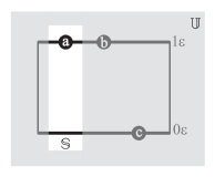
Figure 2: A bipartite system described by two level of energy: $\left\{0\varepsilon,1\varepsilon\right\}$. The universe $\mathbb{U}$ consist three particles $\left\{a,b,c\right\}.$ We choose our system as a subset $\mathbb{S}\subset\mathbb{U}$, which contains $\left\{a\right\}.$ The environment is then the complement $\bar{\mathbb{S}}$ containing $\left\{b,c\right\}$.

In the canonical case, energy can flow between $\mathbb{S}$ and $\bar{\mathbb{S}}$, which indicate an interaction between them. Hence, the total energy of $\mathbb{S}$ is not conserved, so in general, we release the microcanonical constraint (11):

$$E_{+}^{\left(j\right)}=\sum_{i=1}^{2}E_{i}^{\left(j\right)}.$$ (12)

Nevertheless, the microstates $\left\{E_{1}^{\left(j\right)},E_{2}^{\left(j\right)}\right\}$ still need to give the ’correct’ macrostate as a constraint equation:

$$\overline{E}=\sum_{j}^{n}p_{j}E_{+}^{\left(j\right)},\qquad n<\infty,$$

with $p_{j}$ is the canonical distribution function. It should be kept in mind that neither $\mathbb{S}$ nor $\bar{\mathbb{S}}$ is microcanonical, which means neither have equal weight for their microstates; $p_{j}\neq$ constant.

Provided that we know exactly all the possible microstates of the universe $\mathbb{U}$, theoretically, we could obtain the exact canonical probability distribution, given a subsystem $\mathbb{S}\subset\mathbb{U}$. The (normalized) probability distribution for microstate $j$ is:

$$p_{j}=\frac{W^{\left(j\right)}}{\sum_{k}W^{\left(k\right)}},$$

with $\sum_{k}W^{\left(k\right)}$ is the sum of all possible microstates of system $\mathbb{S}$.

An important point we want to emphasize is: knowing all possible microstates of the (isolated) universe $\mathbb{U}$ (which mean knowing $\mathbb{X}_{U}$), then choosing a specific subsystem $\mathbb{S}\subset\mathbb{U}$ (which means knowing $\mathbb{X}_{S}$), then we could obtain exactly the weight / probability distribution $p_{j}^{\left(S\right)}$ for each distinct microstate inside $\mathbb{X}_{S}$, by using the fundamental postulate on $\mathbb{X}_{U}$. This is analog with obtaining a density matrix from a pure state of the universe by tracing out parts of the Hilbert space in quantum mechanics key-2.6 . However, knowing all the possible microstates of the universe is an excessive requirement, therefore we simplify the case by taking an appropriate limit. Given a distribution $p_{j}^{\left(S\right)}$ for our canonical system $\mathbb{S}$, which could be any well-defined distribution, from Kronecker-delta to homogen distribution, for a limit where the environment is much more larger than the observed system, $\bar{\mathbb{S}}\ggg\mathbb{S}$, the most frequent distribution to occur is key-2.10 :

$$p_{j}=g^{\left(j\right)}\exp\left(\beta E_{+}^{\left(j\right)}\right).$$ (13)

Moreover, for a limit where we have large number of energy level and particles, $E_{+}\approxeq E_{+}^{\left(j_{max}\right)}.$ Therefore, if the environment is much more larger than the canonical system, and the energy levels of the system is very dense with a large number of particles, we can safely use (13) as the probability distribution which is responsible for the macrostate $\bar{E}.$ $\beta$ is the Lagrange multiplier related to the microcanonical constraint, which can be defined as the inverse temperature. See key-2.11 for a detailed derivation.

For the canonical case, each microstates could have different weight, and this will result in the existence of the most probable reduced-microstate to occur. In other words, the variance, standard deviation, and fluctuation of energy in the canonical case, in general, are not zero. But in the limit of large number of energy levels and particles, the standard deviation of energy $\sigma_{E}\ll\overline{E},$ therefore, the fluctuation is, effectively, zero. See key-2.8 ; key-2.9 ; key-2.10 ; key-2.11 for standard basic definitions in statistical mechanics.

II.3.2 Grandcanonical case and particle fluctuation.

The most general ensemble case in statistical mechanics is the grandcanonical case, where number of partitions and total energy of the system is not conserved: $\triangle E\neq 0,$ $\triangle N\neq 0$. We release the canonical constraint (12), which contains the information of the number of partitions of the system. This means, we allow the change in the number of partitions, which is two in our previous binary-partition example in the begining of Subsection II A:

$$E_{+}^{\left(j,n\right)}=\sum_{i=1}^{n}E_{i}^{\left(j\right)},$$

(see equation (11) and then compare them).

Let us define an open systems $\mathbb{S}^{\prime}$ inside $\mathbb{U}$ as the collection of all possible subsets of $\mathbb{U}:$ $\mathbb{S}^{\prime}=\left\{s_{i}\left|a\in s_{i};a\in\mathbb{U}\right.\right\},$ $s_{i}\in\mathbb{U}$. These subsets $s_{i}$ are naturally all the possible grandcanonical microstates of our open system $\mathbb{S}$. It is clear that the grandcanonical microstates do not only consist the canonical microstates, but also other canonical microstates with different number of particles. We need to add all of these collections of canonical microstates with different numbers of particles to obtain all possible grandcanonical microstates.

An exact grandcanonical distribution can be obtained by counting procedure, but since it is not really effective to do the calculation this way, we simplify the case just as the previous canonical case. In the limit where the environment is much larger than the grandcanonical system, and the level energy of the system is very dense with a large number of particles, the grandcanonical probability distribution responsible for the macrostate $\overline{E}$ is:

$$P_{\left(j,n\right)}=g^{\left(j\right)}\exp\left(\mu\beta n+\beta E_{+}^{\left(j\right)}\right),$$

with $\mu$ is another Lagrange multiplier related to the canonical constraint (fixing the number of particles), defined as the chemical potential key-2.11 . In the limit of large number of energy levels and particles, the standard deviation of particle’s number $\sigma_{n}\ll\overline{N},$ therefore, the particle fluctuation is, again, effectively zero.

III Applying coarse-graining to gravity

In this section, we apply our coarse-graining proposal described in Section II to discrete gravity. The main idea proposed by the theory of general relativity is: gravity is geometry key-4.2 ; key-4.1 , and therefore, coarse-graining gravity is coarse-graining geometry. In the first subsection, we will start with coarse-graining a 1-dimensional segment, to give a clear insight of the procedure. In the second subsection, we will give restrictions which are related to the cut-offs in the theory. We carry our procedure in a microcanonical framework, but we will generalize to general ensembles, this is done in the third subsection of this part. At last, we will coarse-grain higher dimensional geometries, which are areas and volumes. The dynamics has not been included in our work.

III.1 (1+1) D: Coarse-graining segments

III.1.1 Transformation to the center-of-mass coordinate

For the moment, let us work in $(1+1)$-dimension, where the spatial slice is a 1-dimensional geometrical object. Let us suppose that we have a system containing two coupled segments. Written in the coordinate-free variables, the system has three degrees of freedom: $\left\{\left|\mathbf{l}_{1}\right|,\left|\mathbf{l}_{2}\right|,\phi_{12}\right\}$ key-7 . $\left|\mathbf{l}_{1}\right|,\left|\mathbf{l}_{2}\right|$ are the lengths of the two segments, while $\phi_{12}$ is the angle between them. Following the procedure proposed in Section II, to coarse-grain the system means treating the system as a single segment containing only single degrees of freedom. The first step of this coarse-graining procedure is to obtain the transformation to the ’center-of-mass’ coordinate. Let us return to the non-coordinate-free variables, where we describe the system in a vectorial way, $\left\{\mathbf{l}_{1},\mathbf{l}_{2}\right\}$ key-7 . Written in vectors, the transformation to obtain the center-of-mass coordinate, $\left\{\mathbf{l}_{+},\mathbf{l}_{-}\right\}$, is obvious:

$$\mathbf{l}_{\pm} = \mathbf{l}_{1}\pm\mathbf{l}_{2},$$ (14)

These are similar to the transformation (1) defined in Subsection II A.

The next step is to obtain the coordinate-free version of $\left\{\mathbf{l}_{+},\mathbf{l}_{-}\right\}$. It could be done by taking the norms and the 2D dihedral angle between these two 1-forms, as defined in key-7 . The ’center-of-mass’ coordinate-free variables are written as $\left\{\left|\mathbf{l}_{+}\right|,\left|\mathbf{l}_{-}\right|,\alpha\right\}$, where the transformation is:

$$\left|\mathbf{l}_{\pm}\right| = \sqrt{g\left(\mathbf{l}_{1}\pm\mathbf{l}_{2},\mathbf{l}_{1}\pm\mathbf{l}_{2}\right)},$$ (15)

$$\cos\alpha = \frac{g\left(\mathbf{l}_{1}+\mathbf{l}_{2},\mathbf{l}_{1}-\mathbf{l}_{2}\right)}{\left|\mathbf{l}_{1}+\mathbf{l}_{2},\right|\left|\mathbf{l}_{1}-\mathbf{l}_{2}\right|},$$ (16)

$\alpha$ is the 2D angle between segment $\left|\mathbf{l}_{+}\right|$ and $\left|\mathbf{l}_{-}\right|$, and $g$ is a Euclidean metric, see key-7 for a detail explanation. In fact, we could directly define transformation (15)-(16) as the transformation to the center-of-mass variables without using the vectorial transformation (14); we use the vectorial form just as a simple way to derive this transformation.

It should be kept in mind that $\left\{\left|\mathbf{l}_{1}\right|,\left|\mathbf{l}_{2}\right|,\phi_{12}\right\}$ and $\left\{\left|\mathbf{l}_{+}\right|,\left|\mathbf{l}_{-}\right|,\alpha\right\}$ describe the same system, but they use different choice of variables: the first one use the length of each individual segments and the angle between them, while the later use the total length and their difference, with the angle between them.

Now, having the ’center-of-mass’ variables written in a coordinate-free way, the coarse-graining procedure is to be defined straightforwardly.

III.1.2 Geometrical setting and terminologies

Following an example in key-7 , for the moment, we take a compact, simply-connected slice as the foliation of a discrete spacetime $\mathcal{M}_{\Delta}$, we call this spatial slice $\mathcal{S}_{\triangle}^{1};$ which is topologically a boundary of an $n$-polygon. Each segment is a portion of a real line $\left[0,\left|\mathbf{l}_{i}\right|\right]\subset\mathbb{R}_{i}^{1}.$ The length of each segment is defined as a scalar $\left|\mathbf{l}_{i}\right|.$ We call each segment of $\mathcal{S}_{\triangle}^{1}$ as a partition of the whole system.

Suppose we have $\mathcal{S}_{\triangle}^{1}$ discretized by six partitions as in FIG. 3.

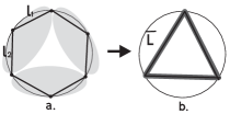
Figure 3: (a) is $\mathcal{S}_{\triangle=6}^{1}$ , a hexagon containing by a six segments. It is coarse-grained into (b), $\mathcal{S}_{\triangle=3}^{1}$ , where it only contains three segments by collecting each two adjacent segments together, for example, $\left|\mathbf{l}_{1}\right|$ and $\left|\mathbf{l}_{2}\right|$. Averaging over all the possible values of $\left|\mathbf{l}_{1}\right|$ and $\left|\mathbf{l}_{2}\right|$ gives the coarse-grained length $\overline{\left|\mathbf{L}\right|}$.

In analogy with the coarse-graining of many-body problem described in Section II, we coarse-grained $\mathcal{S}_{\triangle}^{1}$ so that it only contains three partitions, by collecting each two adjacent segments together. We call the discrete geometrical object containing six and three partitions as a hexagon $\mathcal{S}_{\triangle=6}^{1}$ and triangle $\mathcal{S}_{\triangle=3}^{1}$ , respectively. $\mathcal{S}_{\triangle=6}^{1}$ is the fine-grained state and triangle $\mathcal{S}_{\triangle=3}^{1}$ is the coarse-grained state. See FIG. 3.

Let us focus to the two adjacent segments of $\mathcal{S}_{\triangle=6}^{1}$, they construct a system containing two coupled segments, say, system $\mathbb{L}$, for ’length’. $\mathbb{L}$ is described by three degrees of freedom, denoted by the configuration $\left\{\left|\mathbf{l}_{1}\right|,\left|\mathbf{l}_{2}\right|,\phi_{12}\right\},$ or $\left\{\left|\mathbf{l}_{+}\right|,\left|\mathbf{l}_{-}\right|,\alpha\right\}$, written in the center-of-mass variables. We call the configuration $\left\{\left|\mathbf{l}_{1}\right|,\left|\mathbf{l}_{2}\right|,\phi_{12}\right\}$ or $\left\{\left|\mathbf{l}_{+}\right|,\left|\mathbf{l}_{-}\right|,\alpha\right\}$ as the correct microstate of system $\mathbb{L}$. Any possible configuration of $\mathbb{L}$, which we denote as $\left\{\left|\mathbf{l}_{1}^{\left(j\right)}\right|,\left|\mathbf{l}_{2}^{\left(j\right)}\right|,\phi_{12}^{\left(j\right)}\right\}$ or $\left\{\left|\mathbf{l}_{+}^{\left(j\right)}\right|,\left|\mathbf{l}_{-}^{\left(j\right)}\right|,\alpha^{\left(j\right)}\right\},$ for $j\in\mathbb{Z}$, is defined as the $j^{th}$-microstate. The collection of all possible microstates construct a sample space $\mathbb{X}_{L}$ of the system $\mathbb{L}$.

Now let us use the center-of-mass variables $\left\{\left|\mathbf{l}_{+}\right|,\left|\mathbf{l}_{-}\right|,\alpha\right\}$ as the correct-microstate. We want to treat $\mathbb{L}$ as a coarser system containing only a single segment. A natural way to do this is to describe the system using variable $\left|\mathbf{l}_{+}\right|$, by transformation (15). $\left|\mathbf{l}_{+}\right|$ is the correct reduced-microstate, which is the total length of the segment: the norm of the sum of segment $\mathbf{l}_{1}$ and $\mathbf{l}_{2}$:

$$\left|\mathbf{l}_{+}\right|=\left|\mathbf{l}_{1}+\mathbf{l}_{2}\right|,$$

see FIG. 4.

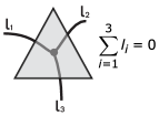
Figure 4: A closed triangle in 2-dimensional space is formed by three vectors $\mathbf{l}_{1}$, $\mathbf{l}_{2}$, $\mathbf{l}_{12}\in T_{p}M\sim\mathbb{R}^{2}$, which must satisfied a closure condition (sometimes called as Gauss constraint in physics term) $\mathbf{l}_{1}+\mathbf{l}_{2}+\mathbf{l}_{12}=0$. Three segments $\left|\mathbf{l}_{1}\right|$, $\left|\mathbf{l}_{2}\right|$, and $\left|\mathbf{l}_{12}\right|$, each of them belongs to a distinct $\mathbb{R}_{i}^{1}$, formed a closed triangle $\mathbf{a}$, which is in fact a portion of a flat 2-dimensional space $\mathbb{R}^{2}.$ Then we can think segment $\left|\mathbf{l}_{1}\right|$, $\left|\mathbf{l}_{2}\right|$, and $\left|\mathbf{l}_{12}\right|$ are embedded on a common $\mathbb{R}^{2}.$ Using this triangle, we can construct 2-dimensional vectors describing each segments: $\mathbf{l}_{1}$, $\mathbf{l}_{2}$, and $\mathbf{l}_{12}$ $\in T_{p}M\sim\mathbb{R}^{2}.$ In other words, we assume the segments $\mathbf{l}_{1}$, $\mathbf{l}_{2}$, and $\mathbf{l}_{12}$ are embedded in a one dimensional higher, flat manifold, which is the triangle $\mathbf{a}$. This assumption is reasonable because before doing coarse-graining on the slice, firstly we need to coarse-grain the bulk, which means the bulk where the fine-grained slice lied must already be flatten key-4.3 . Using the Minkowski theorem in $\mathbb{R}^{2}$, we have $\mathbf{l}_{1}+\mathbf{l}_{2}+\mathbf{l}_{12}=0$, where $\mathbf{l}_{1}$, $\mathbf{l}_{2}$, and $\mathbf{l}_{12}$ formed a closed triangle.

Doing the same way to any microstate $\left\{\left|\mathbf{l}_{+}^{\left(j\right)}\right|,\left|\mathbf{l}_{-}^{\left(j\right)}\right|,\alpha^{\left(j\right)}\right\},$ we obtain all possible reduced $j^{th}$-microstate, $\left|\mathbf{l}_{+}^{\left(j\right)}\right|$:

$$\left|\mathbf{l}_{+}^{\left(j\right)}\right|=\sqrt{\left|\mathbf{l}_{1}^{\left(j\right)}\right|^{2}+\left|\mathbf{l}_{2}^{\left(j\right)}\right|^{2}-2\left|\mathbf{l}_{1}^{\left(j\right)}\right|\left|\mathbf{l}_{2}^{\left(j\right)}\right|\cos\phi_{12}^{\left(j\right)}}.$$ (17)

We define the macrostate $\overline{\left|\mathbf{L}\right|}$ as an average value over all possible configuration under a weight/probability distribution $p_{j}:$

$$\overline{\left|\mathbf{L}\right|}=\sum_{j}p_{j}\left|\mathbf{l}_{+}^{\left(j\right)}\right|,\qquad j\in\mathbb{Z}.$$ (18)

The coarse-grained length is defined as the macrostate, relative to fine-grained length, which is defined to be sum of the norms of the $\mathbf{l}_{1}$ and $\mathbf{l}_{2}$:

$$\left|\mathbf{l}\right|_{+}=\left|\mathbf{l}_{1}\right|+\left|\mathbf{l}_{2}\right|.$$ (19)

See FIG. 4.

In the statistical mechanics point of view, we can only have certain information about the macrostate $\overline{\left|\mathbf{L}\right|}$, without knowing the details of the fine degrees of freedom, i.e., we do not know the correct values of $\left\{\left|\mathbf{l}_{1}\right|,\left|\mathbf{l}_{2}\right|,\phi_{12}\right\}$, in this case. But we can assume them to be some numbers, so that they give the correct average value under a specific probability distribution, which is the macrostate $\overline{\left|\mathbf{L}\right|}$.

In the end, by taking the full-discretized object mentioned in the beginning of this section, we obtain the coarse-grained spatial slice; $\mathcal{S}_{\triangle=3}^{1}$, which is the macrostate: an average over all possible fine-grained slices, the microstates $\mathcal{S}_{\triangle=6}^{1}$.

III.2 Restrictions

III.2.1 Bounds on informational entropy

We have already reviewed the definition of informational entropy in Subsection II B. Now we will apply this to coarse-grained discrete geometries. We only use Shannon entropy, since we are dealing with discrete system.

Lower bound entropy.

To prevent divergencies in the infinitely-small scale limit, as explained in Subsection II B, we need to give first restriction to the sample space $\mathbb{X}_{\mathbf{L}}.$ This results in the countability of all the possible microstates, as well as the discreteness in the sample space. The physical consequence of our first restriction is that all the physical properties -in this case, the properties of the microstates $\left\{\left|\mathbf{l}_{1}\right|,\left|\mathbf{l}_{2}\right|,\phi_{12}\right\},$ must be discrete. This statement is equivalent with the statement: $\left\{\left|\mathbf{l}_{1}\right|,\left|\mathbf{l}_{2}\right|,\phi_{12}\right\}$ can not be infinitesimally-small, there should exist an ultraviolet cut-off which prevent the lengths and angles to be arbitrarily small. This is not a problem in Regge geometry since all the geometrical objects are defined by simplices, which are discrete objects.

We consider the Kronecker-delta distribution as the probability distribution describing a completely-known system with maximal certainty, -a ’pure state’. The Shannon entropy of this pure state is zero, by (4), which is consistent with its physical interpretation.

Therefore, the lower bound of the informational entropy is zero, resulting from the Kronecker-delta probability distribution. This is in analog with the von-Neumann entropy bound on the pure state for the spin-network calculation studied in key-4.3 .

Upper-bound entropy.

To prevent divergencies in the infinitely-large scale limit, we need to give second restriction to the sample space $\mathbb{X}_{\mathbf{L}}.$ Following the reasoning described in Subsection II B, giving the second restriction to our discrete geometry system will results in the finiteness of the number of possible microstates, besides of being countable, due to the first restriction. The physical implication of the second restriction, along with the first restriction, is the properties of microstates $\left\{\left|\mathbf{l}_{1}\right|,\left|\mathbf{l}_{2}\right|,\phi_{12}\right\},$ can not be infinitely large, nor infinitely small. This agrees with the atomism principle: the ’atoms’ of space can not be infinitely large.

We consider the homogen distribution (8), as the probability distribution describing a completely-unknown system with maximal uncertainty, -a ’maximally-mixed’ state. With the first and second restrictions, the entropy of the homogeneous probability distribution from (9) which is $S_{\textrm{max}}=\ln W,$ could be obtained.

In conclusion, with first and second restrictions, we have a well-defined entropy for any probability distribution for our discrete geometry system, within the range defined in (10). See Section II B for a detailed derivation concerning bounds on entropy.

III.2.2 The cut-offs and truncation to the theory

Both the first and second restriction define cut-offs to the properties of the system. To give a well-defined and a consistent lower and upper bound of entropy for the maximal and minimal certainty cases, the sample space $\mathbb{X}_{\mathbf{L}}$ needs to be discrete and finite. Because of this reason, the properties of microstates $\left\{\left|\mathbf{l}_{1}\right|,\left|\mathbf{l}_{2}\right|,\phi_{12}\right\},$ can not be infinitely large, nor infinitely small. These can be geometrically interpreted as a restriction to the range of the length of the segments: the segments can not be infinitely small (they must be discrete) and can not be infinitely large:

$$|\mathbf{l}_{\textrm{min}}|\leq|\mathbf{l}|\leq|\mathbf{l}_{\textrm{max}}|, \mathbf{l}\in\Sigma;\;f:\Sigma\rightarrow\mathbb{Z},$$ (20)

$$|\mathbf{l}_{\textrm{min}}|>0, |\mathbf{l}_{\textrm{max}}|<\infty.$$

$f$ is a bijective map which maps every elements of $\Sigma$ to the set of integer numbers $\mathbb{Z}$. The minimal and maximal values $|\mathbf{l}_{\textrm{min}}|$ and $|\mathbf{l}_{\textrm{max}}|$ are the ultraviolet and the infrared cut-offs which prevent the theory from divergencies. Setting these values, we define a truncation to our theory. Returning back to the discretization of $\mathcal{S}^{1}$ in previous subsection, with these truncations, the refinement must stop at some point; it can not go to arbitrarily small details, and the ’perfect’ circle $\mathcal{S}^{1}$ can never be reached, since it is only an idealization.

III.3 Microcanonical case

As explained in Section II C, the microcanonical ensemble is an ensemble of system which satisfies constraints $\Delta E=0,$ $\triangle N=0$; the amount of energy and number of particles in each microstates are fixed. In analog to the kinetic theory, the reduced-microstates (17) must satisfies the microcanonical constraint for a system of coupled-segments: all the possible reduced-microstate must be equal to the correct reduced-microstate:

$$\left|\mathbf{l}_{+}^{\left(j\right)}\right|=\left|\mathbf{l}_{12}\right|.$$ (21)

It must be noted that with this constraint, the values of $\left|\mathbf{l}_{1}^{\left(j\right)}\right|$, $\left|\mathbf{l}_{2}^{\left(j\right)}\right|$, $\phi_{12}^{\left(j\right)}$ could vary, but their relation (their ’total length’) described in (17) must be equal to the correct reduced microstate $\left|\mathbf{l}_{12}\right|.$ This also can be geometrically interpreted as taking the ’total length’ and number of partition (which is two fine-grained segments for each coarse-grained segment) to be constants.

To conclude this subsection, coarse-graining from $\mathcal{S}_{\triangle=6}^{1}$ to $\mathcal{S}_{\triangle=3}^{1}$ (FIG. 3) means we only know with certainty the macrostate $\overline{\left|\mathbf{L}\right|}$, and lose the information about the correct configuration of microstate $\left\{\left|\mathbf{l}_{1}^{\left(j\right)}\right|,\left|\mathbf{l}_{2}^{\left(j\right)}\right|,\right.$ $\left.\phi_{12}^{\left(j\right)}\right\}$ (which is $\left\{\left|\mathbf{l}_{1}\right|,\left|\mathbf{l}_{2}\right|,\phi_{12}\right\},$ respectively). See FIG. 5.

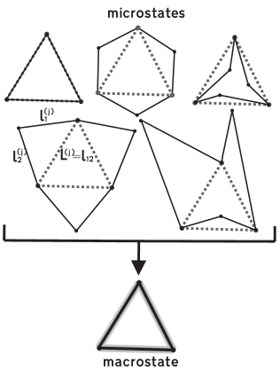
Figure 5: The microcanonical case: Some of the possible microstates $\mathcal{S}_{\triangle=6}^{1}$ which contains six partitions, coarse-grained into a single macrostate $\mathcal{S}_{\triangle=3}^{1}$ , which contains only three partitions. The total length of each two adjacent segments $\left\{\mathbf{l}_{1}^{\left(j\right)},\mathbf{l}_{2}^{\left(j\right)}\right\}$ are equal for each microstates, which is $\mathbf{l}_{12}$.

III.4 General ensemble case

III.4.1 Canonical case and length fluctuation

The canonical ensemble in kinetic theory is an ensemble of systems which only satisfy the constraint $\Delta N=0.$ The energy can flow in and out from each microstate, but the number of partitions is conserved. Using the same analogy here, we define in general the canonical ensemble in the discrete geometrical sense by relaxing the microcanonical constraint (21); in the canonical case, $\left|\mathbf{l}_{+}^{\left(j\right)}\right|$ does not need to be equal to $\left|\mathbf{l}_{12}\right|$:

$$\left|\mathbf{l}_{+}^{\left(j\right)}\right|=\left|\sum_{i=1}^{2}\mathbf{l}_{i}^{\left(j\right)}\right|.$$ (22)

This means the total length of two adjacent segments may vary, as long as averaging all of them still give the macrostate $\overline{\left|\mathbf{L}\right|},$ see FIG. 6.

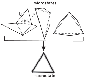
Figure 6: The canonical case: Some of the possible microstates $\mathcal{S}_{\triangle=6}^{1}$ which contains six partitions, coarse-grained into a single macrostate $\mathcal{S}_{\triangle=3}^{1}$ , which contains only three partitions. The total length of each two adjacent segments $\left\{\mathbf{l}_{1}^{\left(j\right)},\mathbf{l}_{2}^{\left(j\right)}\right\}$ may vary. This will lead to a fluctuation of length, since now the microstates $\left|\mathbf{l}_{+}^{\left(j\right)}\right|_{c}$ is not a constant.

Without the microcanonical constraint, we have more possible microstates, while the first and second restriction are still maintained. In this case, we have fluctuations of length. The variance of the length, in general, is not zero; this will depend on the probability density. It is clear that for the Kronecker delta, the variance is zero, no matter if the case is canonical or microcanonical. This condition is consistent with the physical interpretation, since in the Kronecker delta distribution, we only have one possible microstate, so there is no fluctuation of length.

III.4.2 Grandcanonical case, length, and ’particle’ fluctuations

The most general ensemble in kinetic theory is the grandcanonical ensemble, where we have no restriction on $\Delta E$ and $\Delta N$. In the two previous ensembles, the number of partitions is fixed: two partitions for each coarse-grained segment of the discretization. Now, we release this restriction; the relation (22) of the canonical case becomes:

$$\left|\mathbf{l}_{+}^{\left(j,n_{j}\right)}\right|_{g}=\left|\sum_{i=1}^{n_{j}}\mathbf{l}_{i}^{\left(j\right)}\right|,$$ (23)

which means, each different microstate $\left|\mathbf{l}_{+}^{\left(j\right)}\right|_{g}$ will have degeneracy in terms of number of partitions. See FIG. 7.

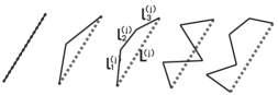
Figure 7: Each different microstate $\left|\mathbf{l}_{+}^{\left(j\right)}\right|_{g}$ has degeneracy in terms of number of partitions, which is the number of segments.

The microstate of the grandcanonical system also depends on the number of partitions $n_{j}$, which in statistical mechanics, is usually called as the occupation number. The average length is given by:

$$\overline{\left|\mathbf{L}\right|}=\sum_{j}^{W}P_{j}\left|\mathbf{l}_{+}^{\left(j,n_{j}\right)}\right|_{g},$$

with $P_{j}$ is the grand-canonical distribution function, $W$ is the number of all possible microstates, and $n_{j}$ is the number of partition on each microstate $\left|\mathbf{l}_{+}^{\left(j\right)}\right|_{g}.$ We can collect all microstates having the same occupation numbers $n_{j}$. The idea is similar to collecting states which have same wave-number $k$ when we define the Fock space in quantum mechanics. Furthermore, we could defined the average occupation number:

$$\bar{n}=\sum_{k}^{\mathcal{W}}\mathcal{P}_{k}n_{k}.$$

The probability distribution $\mathcal{P}_{k}$ is ’Fourier conjugate’ to $P_{j}$.

Obviously, in the grand canonical case, we have length fluctuation, using the same definition as in the canonical case. But there is also another fluctuation: the fluctuation of the number of partitions, or, in the statistical mechanics language, ’particle number’ fluctuation. The variance, standard deviation, and fluctuation can be obtained using the standard formula; if $P_{j}$ is the Kronecker-delta distribution, then the variance this is similar to the previous cases. See FIG. 8.

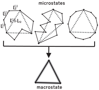
Figure 8: The grandcanonical case: Some of the possible microstates $\mathcal{S}_{\triangle=6}^{1}$ which can contain any number of partitions, coarse-grained into a single macrostate $\mathcal{S}_{\triangle=3}^{1}$, which contains only three partitions. This will lead to a fluctuation in the number of partitions, since now the number of partition of each microstates is not a constant. The fluctuation of length also exist, in general.

III.5 Higher dimensional case

In the previous sections, we worked in the (1+1)-dimensional case, and the geometrical object we coarse-grained were collections of segments, a 1-dimensional slice of a 2-dimensional spacetime. In higher dimensions, we could coarse-grain areas and volumes.

In this subsection, we will use the construction of $n$-simplex procedure explained in our earlier work key-7 as a basic property. Another important theorem we will used in this subsection is the Minkowski theorem or the closure constraint key-3.5 ; key-3.26 . It is related to the construction of $p$-simplices embedded in $\mathbb{R}^{n}$. For $p=2,$ it is a construction of a closed triangle from three vectors $\left\{\mathbf{l}_{1},\right.$ $\mathbf{l}_{2},$ $\left.\mathbf{l}_{3}=-\mathbf{l}_{12}\right\}\in\mathbb{R}^{n},$ which satisfy the closure constraint:

$$\sum_{i=1}^{3}\mathbf{l}_{i}=0.$$

Using physical terminology, this constraint is called the gauge invariance condition. It is already explained in key-7 that closure condition will cause triangle-inequality, but not vice-versa. See FIG. 4 as an example. We will use this property to generalize our result in higher dimension.

III.5.1 (2+1) D: Coarse-graining area

In the (2+1) D theory, the slice $\Sigma$ of a 3D manifold $\mathcal{M}$ is a 2-dimensional surface, therefore in this case, we will be coarse-graining the area of surfaces. Let a discretized surface be triangulated by three triangles as illustrated in FIG. 9(a).

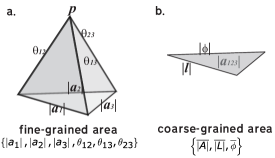
Figure 9: (a) is a portion of a discretized surface triangulated by three triangles. Coarse-graining the area of the surface is defined as treating these three triangles as one system: by substituting them with a single and flat triangle in figure (b), while keeping the boundary (segments $\left|\mathbf{l}_{1}\right|$, $\left|\mathbf{l}_{2}\right|$, $\left|\mathbf{l}_{3}\right|$) fixed. This transformation is known as 3-1 Pachner move.

Let us apply the 3-1 Pachner move. This configuration contains six degrees of freedom, we can choose them to be written as $\left\{\left|\mathbf{a}_{1}\right|,\left|\mathbf{a}_{2}\right|,\left|\mathbf{a}_{3}\right|,\theta_{12},\theta_{23},\theta_{13}\right\}$ to prevent ambiguities: the system contains three triangles with area $\left|\mathbf{a}_{i}\right|$ and coupling constant $\theta_{ij}$ between each two of them key-7 . From the information of $\left\{\theta_{12},\theta_{23},\theta_{13}\right\}$ (the angles between two triangles, -3D dihedral angles), using the inverse dihedral angle relation key-7 :

$$\cos\phi_{ij}=\frac{\cos\theta_{ij,k}-\cos\theta_{ik,j}\cos\theta_{kj,i}}{\sin\theta_{ik,j}\sin\theta_{kj,i}},$$ (24)

we could obtain $\left\{\phi_{12},\phi_{23},\phi_{13}\right\}$ (the angles between two segments, -2D dihedral angles), and then calculate the deficit angle on the hinge (the point $p$ in FIG. 9(a)):

$$\delta\phi=2\pi-\sum_{i=1}^{3}\phi_{i},$$

which defines the intrinsic 2D curvature of the surface. These information completely determine the discretized surface. It must be noted that we did not use vectorial objects to define the surface, all the variables we have are written in a coordinate-free way, i.e., they are scalars. See FIG. 10.

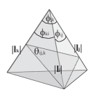
Figure 10: Given angles $\phi_{ij}$, $\phi_{ik}$, $\phi_{jk}$ at point $p$ of a tetrahedron, we could obtain the dihedral angle $\theta{}_{ij,k}$. In fact, $\theta{}_{ij,k}$ is only $\phi_{ij}$ projected on the plane normal to segment $\left|\mathbf{l}_{k}\right|$.

The next step is to obtain ’transformation’ to the ’center-of-mass’ variables, the ’center-of-mass’ of the system is a single triangle, obtained by ’summing-up’ the three triangles of 3-1 Pachner move. This ’center-of-mass’ variables can be written as $\left\{\left|\mathbf{a}_{123}\right|,\left|\mathbf{l}\right|,\phi,\boldsymbol{\alpha}\right\},$ with $\left|\mathbf{a}_{123}\right|$ is the ’total area’: the norm of the sum of areas $\mathbf{a}_{1}$, $\mathbf{a}_{2}$, and $\mathbf{a}_{3}$; $\left|\mathbf{l}\right|$ and $\phi$ are, respectively, one of the segment and 2D angle of this ’center-of-mass’ triangle, and $\boldsymbol{\alpha}$ are the variables which we are going to coarse-grained (we could choose it to be $\boldsymbol{\alpha}=\left(\left|\mathbf{a}_{12}\right|,\left|\mathbf{a}_{1}\right|,\alpha\right),$ with $\alpha$ is the angle between triangles $\left|\mathbf{a}_{12}\right|$ and $\left|\mathbf{a}_{1}\right|$, but they are not so important since we are going to neglect them all by the coarse-graining procedure).

For the next step, we would like to obtain the formula relating the total area $\left|\mathbf{a}_{123}\right|$ with the fine-grained areas $\left|\mathbf{a}_{i}\right|.$ Let us return to the vectorial notation $\mathbf{a}_{i}$. In the vectorial picture, it is obvious that the three triangles of the discretized surface and the triangle of the total area can be arranged so that they construct a flat tetrahedron, in the same way four 2-simplices constructed a 3-simplex. This flat tetrahedron is embedded in $\mathbb{R}^{3}$ (in fact, it is a portion of $\mathbb{R}^{3}$). The three triangles and the total triangle form the surface of the tetrahedron (which is automatically embedded on $\mathbb{R}^{3}$). Therefore, we could describe these triangles vectorially, using a 2-form $\mathbf{a}_{i}\in\Omega^{2}\left(\mathbb{R}^{3}\right)$ (with $\Omega^{2}\left(\mathbb{R}^{3}\right)$ is the space of $2$-form over $\mathbb{R}^{3}$), such that their norms give the same norms $\left|\mathbf{a}_{i}\right|$ as before. Using the closure constraint (or Minkowski theorem in $\mathbb{R}^{3}$ ($\Omega^{2}\left(\mathbb{R}^{3}\right)$ is isomorphic to $\mathbb{R}^{3}$)), we have the gauge invariance condition, for the four triangles to form a closed tetrahedron in $\mathbb{R}^{3}$:

$$\sum_{i=1}^{4}\mathbf{a}_{i}=0,$$ (25)

which in our case, can be written as:

$$\mathbf{a}_{4}=-\mathbf{a}_{123}=-\left(\mathbf{a}_{1}+\mathbf{a}_{2}+\mathbf{a}_{3}\right).$$ (26)

See FIG. 11.

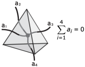
Figure 11: The Minkowski theorem in $\mathbb{R}^{3}$, a closed surface of a tetrahedron must satisfy gauge invariance condition.

Taking the norm of equation (26), the ’transformation’ relation we would like to obtain is:

$$\left|\mathbf{a}_{123}\right| = \sqrt{\sum_{i=1}^{3}\left|\mathbf{a}_{i}\right|^{2}-2\sum_{\binom{i<j}{i=1}}^{3}\left|\mathbf{a}_{i}\right|\left|\mathbf{a}_{j}\right|\cos\theta_{ij}},$$ (27)

$$\boldsymbol{\alpha}=\boldsymbol{\alpha}\left(\left|\mathbf{a}_{1}\right|,\left|\mathbf{a}_{2}\right|,\left|\mathbf{a}_{3}\right|,\theta_{12},\theta_{23},\theta_{13}\right),$$

with $\theta_{ij}$ are the 3D dihedral angles. The other variables $\left|\mathbf{l}\right|,\phi$ can be obtained given the information of $\left\{\left|\mathbf{a}_{1}\right|\right.,$ $\left|\mathbf{a}_{2}\right|,$ $\left|\mathbf{a}_{3}\right|,$ $\theta_{12}$, $\theta_{23},$ $\left.\theta_{13}\right\}$, see key-7 . Similar with the lower dimension analog, we use the vectorial form just as a simple way to derive this transformation.

At a first glance, formula $\left(\ref{eq:16}\right)$ seems to be an ’extrinsic’ relation, since $\cos\theta_{ij}$ is an extrinsic property, relative to the 2D surface (the angle $\theta_{ij}$ does not ’belong’ to the 2D surface $\Sigma$). But by using the remarkable dihedral angle formula, the 3D dihedral angles of the tetrahedron can be written as functions of the angles between segments using its inverse formula (24). See FIG. 10. For a detailed explanation about these angles, see key-7 ; key-3.28 ; key-3.29 . Therefore, it is clear that formula $\left(\ref{eq:16}\right)$ is purely intrinsic to the 2D surface, it does not depend on the embedding in $\mathbb{R}^{3},$ we only use $\mathbb{R}^{3}$ to help us to derive relation (27) in an easy way.

Now, as a 2-dimensional analog to the coarse-graining in 1-dimension carried in Subsection III A, we define the statistical mechanics terminologies. Let us called $\left\{\left|\mathbf{a}_{123}\right|,\left|\mathbf{l}\right|,\phi,\boldsymbol{\alpha}\right\}$ as the correct microstate, and $\left\{\left|\mathbf{a}_{123}^{\left(k\right)}\right|,\left|\mathbf{l}^{\left(k\right)}\right|,\phi^{\left(k\right)},\boldsymbol{\alpha}^{\left(k\right)}\right\},$ as the $k^{th}$-microstate. We reduce the degrees of freedom away by removing $\boldsymbol{\alpha}$ and defining the correct reduced-microstate as $\left\{\left|\mathbf{a}_{123}\right|,\left|\mathbf{l}\right|,\phi\right\},$ and the $k^{th}$ reduced-microstate as $\left\{\left|\mathbf{a}_{123}^{\left(k\right)}\right|,\left|\mathbf{l}^{\left(k\right)}\right|,\phi^{\left(k\right)}\right\},$ satisfying:

$$\left|\mathbf{a}_{123}^{\left(k\right)}\right|=\sqrt{\sum_{i=1}^{3}\left|\mathbf{a}_{i}^{\left(k\right)}\right|^{2}-2\sum_{\binom{i<j}{i=1}}^{3}\left|\mathbf{a}_{i}^{\left(k\right)}\right|\left|\mathbf{a}_{j}^{\left(k\right)}\right|\cos\theta_{ij}^{\left(k\right)}},$$ (28)

$$\left|\mathbf{l}^{\left(k\right)}\right| = \left|\mathbf{l}_{12}^{\left(k\right)}\right|,$$

$$\phi^{\left(k\right)} = f\left(\left|\mathbf{l}_{12}^{\left(k\right)}\right|,\boldsymbol{\alpha}^{\left(k\right)}\right).$$

The coarse-grained triangle is defined as the macrostate of the system $\left\{\overline{\left|\mathbf{A}\right|},\overline{\left|\mathbf{L}\right|},\bar{\phi}\right\}$ :

$$\overline{\left|\mathbf{A}\right|} = \sum_{k}p_{k}\left|\mathbf{a}_{123}^{\left(k\right)}\right|,$$

$$\overline{\left|\mathbf{L}\right|} = \sum_{k}p_{k}\left|\mathbf{l}^{\left(k\right)}\right|,$$

$$\bar{\phi} = \sum_{k}p_{k}\phi^{\left(k\right)},$$

which is an average value over all possible reduced-microstates (28). We called $\overline{\left|\mathbf{A}\right|}$ as the coarse-grained area, while the fine-grained area is the ’sum of the norms’: $\sum_{i=1}^{3}\left|\mathbf{a}_{i}\right|$; the area of the ’correct’ microstate. The microcanonical case is described by the constraint:

$$\left|\mathbf{a}_{123}^{\left(k\right)}\right|=\left|\mathbf{a}_{123}\right|.$$

Now, what is the geometrical interpretation of this coarse-graining method? First, we look at formula (27), which looks like the total ’lagrangian’ of the system: $\sum_{i=1}^{3}\left|\mathbf{a}_{i}\right|^{2}$ looks like the ’kinetic’ part, while the $\left|\mathbf{a}_{i}\right|\left|\mathbf{a}_{j}\right|\cos\theta_{ij}$ looks like the ’interaction’ part between fields $\left|\mathbf{a}_{i}\right|$ and $\left|\mathbf{a}_{j}\right|$, with $\cos\theta_{ij}$ as the ’coupling constant’. We can think the discretized surface as a many-body system containing (in this case) three ’quanta’ of area, with interactions among them. The measure of how strong are the interactions is described by the ’couplings’: the angles between these quanta of area, which in turn, by (24), is related to the intrinsic curvature of the surface. In this sense, we could think the intrinsic curvature as an emergent property of a many-body system; which measures the intensity of the interaction among the ’quanta’ of areas of the surface key-7 . Small curvature (small deficit angle, which means the coupling, -the cosine of the dihedral angle between two ’quanta’ $\approx 1$) gives maximal interaction between the ’quanta’ of space, while large curvature (large deficit angle, which means the coupling $\approx 0$) gives minimal interaction.

Second, by coarse-graining, we treat the system (in our case) as a single ’particle’ of a area, which means we loose the information about the individual “atoms” and also the interaction among them. This interpretation is consistent with the fact that by coarse-graining, we loose the information about the intrinsic curvature of the slice, since a collection of several ’interacting’ triangles is replaced by a single flat triangle. See FIG. 12 for a coarse-grained area example.

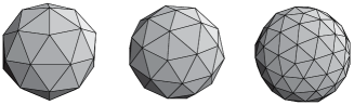
Figure 12: Coarse-graining areas will correspond in loosing the intrinsic curvature of the surface.

As a last point, we need to generalize these results to a more general statistical ensembles: for the canonical case we have $\left|\mathbf{a}_{123}^{\left(k\right)}\right|=\left|\sum_{i=1}^{3}\mathbf{a}_{i}^{k}\right|,$ while for the grandcanonical case we have $\left|\mathbf{a}_{123}^{\left(k\right)}\right|=\left|\sum_{i=1}^{n_{k}}\mathbf{a}_{i}^{k}\right|$, both are, in general, not equal to $\left|\mathbf{a}_{123}\right|$. The area and particle number fluctuations are defined in the same way as in the 1-dimensional case. We should remember that we still have freedom to coarse-grain length just as in the previous section, but it can only be done after we coarse-grain the surface.

III.5.2 (3+1) D: Coarse-graining volume

Let us go to the real world by adding one dimensional higher. In (3+1) dimensions we will discuss two cases: the 4-1 and 3-2 moves. The slice $\Sigma$ of a 4D manifold $\mathcal{M}$ is a 3-dimensional space, therefore in this case, we will coarse-grain volumes of space.

4-1 Pachner moves case.

We take a portion of 3D space discretized by four tetrahedra, illustrated in FIG. 13, which is the 4-1 Pachner move.

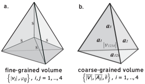
Figure 13: (a) is a portion of a discretized space triangulated by four tetrahedra. Coarse-graining the volume of the space is defined as treating these four tetrahedra as one system: by substituting them with a single, flat tetrahedron in figure (b) while keeping the boundary (triangles $\mathbf{a}_{1}$, $\mathbf{a}_{2}$, $\mathbf{a}_{3}$, $\mathbf{a}_{4}$) fixed. This transformation is known as 4-1 Pachner move.

Each tetrahedron is a portion of an $\mathbb{R}^{3}$ space, which is distinct for each tetrahedron. In the vectorial way, they are described by 3-forms $\mathbf{v}_{i}$, obtained from the wedge product of three segments $\mathbf{l}_{j}$ (see key-7 ), or it can be obtained from the area of the triangles $\mathbf{a}_{j}$. The volume of the tetrahedron is defined by its norm, or by:

$$\left|\mathbf{v}_{i}\right|^{2}=\frac{2}{9}\mathbf{a}_{j}\cdot\left(\mathbf{a}_{k}\times\mathbf{a}_{l}\right),$$ (29)

with $\mathbf{a}_{j}\in\Omega^{2}\left(\mathbb{R}^{3}\right)$ are the 2-simplices: three triangles from all the four which bound the tetrahedron (the closure constraint on $\mathbb{R}^{3}$ (25) guarantees any combination will give the same volume). It must be emphasized here that we are working on a purely Regge geometry picture and we are not going to consider the twisted geometry case in this work. This means we know exactly the shape of the tetrahedra; not only the norm of the areas $\left|\mathbf{a}_{j}\right|$ of the triangles (as in the twisted geometry case), but also the length of each segments of the tetrahedron $\left|\mathbf{l}_{j}\right|$. This is equivalent with having the information about the vectorial triangles $\mathbf{a}_{j}$, which are used to derive the volume of the tetrahedron.

The system in FIG. 13(a) is described by ten degrees of freedom (see key-7 ), we choose the variables to be the individual volumes of tetrahedra and the 4D dihedral angles between them $\left\{\left|\mathbf{v}_{i}\right|,\varphi_{ij}\right\}$, for $i,j=1,2,3,4,\,i\neq j$. Similar to the previous lower-dimensional cases, the next step is to obtain the center-of-mass variables, which are $\left\{\left|\mathbf{v}_{1234}\right|,\left|\mathbf{a}_{i}\right|,\theta,\boldsymbol{\alpha}\right\},$ for $i=1,..,4$. $\left\{\left|\mathbf{v}_{1234}\right|,\left|\mathbf{a}_{i}\right|,\theta\right\}$ describe the center-of-mass tetrahedron: $\left|\mathbf{v}_{1234}\right|$ is the volume, $\left|\mathbf{a}_{i}\right|$ are areas of the external (boundary) triangles, and $\theta$ is one of the six 3D dihedral angles between triangles, while $\boldsymbol{\alpha}$ are four degrees of freedom we are going to coarse-grain.

Using the analogy of the (2+1) case (but it is not really obvious since it would require a 4-dimensional space to imagine this object), the four tetrahedra of the discretized space and the tetrahedron of the total volume can be arranged so that they construct a flat 4-simplex: five 3-simplices (tetrahedra), connected to each other, form a 4-simplex. This flat 4-simplex is a portion of $\mathbb{R}^{4}$. The four tetrahedra with the total tetrahedron is the boundary of the 4-simplex and is automatically embedded on $\mathbb{R}^{4}$. Therefore, we could describe these tetrahedra vectorially, using a 3-form $\mathbf{v}_{i}\in\Omega^{3}\left(\mathbb{R}^{4}\right),$ such that their norms gives the same norms $\left|\mathbf{v}_{i}\right|$ as before.

By the same reasoning with the (2+1)-dimensional case, we have the closure constraint or the Minkowski theorem in $\mathbb{R}^{4}$:

$$\sum_{i=1}^{5}\mathbf{v}_{i}=0,$$ (30)

see FIG. 14.

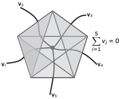
Figure 14: The Minkowski theorem in $\mathbb{R}^{4}$, a closed boundary (hypersurface) of a 4-simplex must satisfy the closure constraint.

The gauge invariance condition (30) can be written as:

$$\mathbf{v}_{1234}=\mathbf{v}_{5}=-\left(\mathbf{v}_{1}+\mathbf{v}_{2}+\mathbf{v}_{3}+\mathbf{v}_{4}\right),$$

therefore, taking the norm, we obtain the formula relating the total volume with the fine-grained volumes:

$$\left|\mathbf{v}_{1234}\right| = \sqrt{\sum_{i=1}^{4}\left|\mathbf{v}_{i}\right|^{2}-2\sum_{\binom{i<j}{i=1}}^{4}\left|\mathbf{v}_{i}\right|\left|\mathbf{v}_{j}\right|\cos\varphi_{ij}},$$ (31)

with $\varphi_{ij}$ is the 4-dimensional angle: the angle between two tetrahedra of a 4-simplex (this ’angle between spaces’ can only exist in spaces with dimension higher than three), see key-7 .

Remarkably, this angle also satisfy the dihedral angle formula in one-dimension higher key-3.28 :

$$\cos\varphi_{ij,k}=\frac{\cos\theta_{ij,k}-\cos\theta_{il,k}\cos\theta_{lj,k}}{\sin\theta_{il,k}\sin\theta_{lj,k}},$$ (32)

with $\theta_{ij,k}$ is the dihedral angle between two triangles $i,j$, located on hinge $k$ key-7 ; key-3.28 . Formula (31) is the 3D analog to (15) and (27), it is also purely intrinsic to the 3D space and does not depend on the embedding in $\mathbb{R}^{4}.$ Using the inverse of (32), we could obtain $\theta_{ij}$, while having the information of $\left\{\left|\mathbf{v}_{i}\right|,\varphi_{ij}\right\}$, we could obtain the external boundary triangles $\left|\mathbf{a}_{i}\right|$.

Now let us define the terminologies; the correct microstate is $\left\{\left|\mathbf{v}_{1234}\right|,\left|\mathbf{a}_{i}\right|,\theta,\boldsymbol{\alpha}\right\},$ for $i=1,..,4$, the $k^{th}$-microstates are $\left\{\left|\mathbf{v}_{1234}^{\left(k\right)}\right|,\left|\mathbf{a}_{i}^{\left(k\right)}\right|,\theta^{\left(k\right)},\boldsymbol{\alpha}^{\left(k\right)}\right\},$ satisfying:

$$\left|\mathbf{v}_{1234}^{\left(k\right)}\right|=\sqrt{\sum_{i=1}^{4}\left|\mathbf{v}_{i}^{\left(k\right)}\right|^{2}-2\sum_{\binom{i<j}{i=1}}^{4}\left|\mathbf{v}_{i}^{\left(k\right)}\right|\left|\mathbf{v}_{j}^{\left(k\right)}\right|\cos\varphi_{ij}^{\left(k\right)}.}$$ (33)

The correct reduced-microstate is $\left\{\left|\mathbf{v}_{1234}\right|,\left|\mathbf{a}_{i}\right|,\theta\right\}$ , and the $k^{th}$-reduced-microstates are $\left\{\left|\mathbf{v}_{1234}^{\left(k\right)}\right|,\right.$ $\left|\mathbf{a}_{i}^{\left(k\right)}\right|,$ $\left.\theta^{\left(k\right)}\right\}.$ The coarse-grained tetrahedron is defined as the macrostate of the system $\left\{\overline{\left|\mathbf{V}\right|},\overline{\left|\mathbf{A}_{i}\right|},\bar{\theta}\right\}$ :

$$\overline{\left|\mathbf{V}\right|} = \sum_{k}p_{k}\left|\mathbf{v}_{1234}^{\left(k\right)}\right|,$$

$$\overline{\left|\mathbf{A}_{i}\right|} = \sum_{k}p_{k}\left|\mathbf{a}_{i}^{\left(k\right)}\right|$$

$$\bar{\theta} = \sum_{k}p_{k}\theta^{\left(k\right)},$$

which is an average value over all possible reduced-microstates. The coarse-grained volume is $\overline{\left|\mathbf{V}\right|}$ , while the fine-grained volume is $\sum_{i=1}^{3}\left|\mathbf{v}_{i}\right|:$ the volume of the ’correct’ microstate. The microcanonical case is described by the constraint:

$$\left|\mathbf{v}_{1234}^{\left(k\right)}\right|=\left|\mathbf{v}_{1234}\right|.$$

For the canonical and grandcanonical case, $\left|\mathbf{v}_{1234}^{\left(k\right)}\right|=\left|\sum_{i=1}^{4}\mathbf{v}_{i}^{\left(k\right)}\right|$ and $\left|\mathbf{v}_{1234}^{\left(k\right)}\right|=\left|\sum_{i=1}^{n_{k}}\mathbf{v}_{i}^{\left(k\right)}\right|$, respectively. The volume and particle number fluctuations are defined in the same way as in the previous cases. We still have freedom to coarse-grain length and area just as in the previous sections, but it must be done in order: first coarse-grain the volume, then the area, and lastly, the length. The reason is because coarse-graining, in a sloppy sense, is ’adding’ $n$-simplices, which are $n-$forms, and in order to add forms, they need to be embedded on a same (cotangent) space first.

The 4-1 Pachner move is simultaneously removing four hinges (segments in (3+1) theory) of the discretized curved space, not only removing a single hinge as in the (2+1) case. What if we only want to coarse-grained single hinge in the (3+1) case? This is the 3-2 Pachner move.

3-2 Pachner moves case.

The simplest coarse-graining case which coarse-grain only a single hinge, is the 3-2 Pachner move. See FIG. 15.

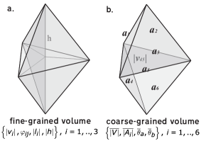
Figure 15: (a) is a portion of a discretized space triangulated by three tetrahedra $\left\{a,b,c\right\}$. The fine grained state contains three tetrahedra glued together on their triangles to contruct a bipyramid - a ’diamond’ in figure (b). The curvature is located on the hinge $\mathbf{h}$ inside it. When we coarse-grained, we loose the hinge, and the coarse-grained bipyramid is now constructed by only two tetrahedra. This transformation is known as 3-2 Pachner move.

FIG. 15(a), which is the ’3’ part of the 3-2 Pachner move, has ten degrees of freedom, this can be easily obtained by calculating the number of segments of this geometrical object. But instead of using these ten segments as the coordinate-free variables, to prevent ambiguities, we use $\left\{\left|\mathbf{v}_{i}\right|,\varphi_{ij},\left|\mathbf{l}_{i}\right|,\left|\mathbf{h}\right|\right\}$, for $i\neq j=1,2,3$; with $\left|\mathbf{v}_{i}\right|$ is the volume of the individual tetrahedron, $\varphi_{ij}$ is the coupling between each two tetrahedra, $\left|\mathbf{l}_{i}\right|$ is one segment of each tetrahedron, and $\left|\mathbf{h}\right|$ is the common internal segment shared by these three tetrahedra. See FIG. 16(a).

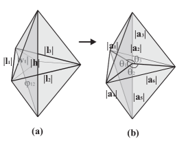
Figure 16: (a) is the ’3’ part of the 3-1 move, described by ten variables. (b) is the ’2’ part of the 3-1 move, described by nine variables.

To coarse-grain FIG. 16(a) means we treat the three coupled tetrahedra as a single system with the surface boundary is held to be constant for a moment. This mean, we kept the nine external segments constructing the ’bipyramid’ to be constants, and we remove the internal segment $\left|\mathbf{h}\right|$ away. But $\left|\mathbf{h}\right|$ is the location of the intrinsic 3D curvature, that is, it defines the dihedral angles of each tetrahedron, say, $\left\{\theta_{1},\theta_{2},\theta_{3}\right\},$ which gives the 3D intrinsic curvature:

$$\delta\theta=2\pi-\sum_{i=1}^{3}\theta_{i}.$$

Therefore, removing $\left|\mathbf{h}\right|$ away will result in the lost of the intrinsic 3D curvature. This condition can be realized by setting $\delta\theta=0,$ so that it is equivalent with introducing a new constraint:

$$\theta_{1}+\theta_{2}+\theta_{3}=0$$ (34)

to the system. With this constraint, the total degrees of freedom of the system in FIG. 16(a) reduces from ten to nine (the ’2’ part of the move), which is exactly the number of segments of a flat, trihedral-bipyramid. We choose the ’center-of-mass’ variables to be $\left\{\left|\mathbf{v}_{123}\right|,\left|\mathbf{a}_{i}\right|,\theta_{j}\right\},$ for $i=1,..,6,$ and $j=1,..,3,$ with $\left|\mathbf{v}_{123}\right|$ is the total volume of the ’center-of-mass’ bipyramid, satisfying:

$$\left|\mathbf{v}_{123}\right| = \sqrt{\sum_{i=1}^{3}\left|\mathbf{v}_{i}\right|^{2}-2\sum_{\binom{i<j}{i=1}}^{3}\left|\mathbf{v}_{i}\right|\left|\mathbf{v}_{j}\right|\cos\varphi_{ij}},\;i,j=1,2,3.$$

$\left|\mathbf{a}_{i}\right|$ are the six external areas of the bipyramid triangles, and $\theta_{j}$ are the three dihedral angles located on the hinge, they determine a segment of a triangle. See FIG. 16(b).

Now let us define the terminologies. Let $\left\{\left|\mathbf{v}_{123}\right|,\left|\mathbf{a}_{i}\right|,\theta_{j}\right\}$ for $i=1,..,6,$ and $j=1,..,3,$ be the correct microstate, then $\left\{\left|\mathbf{v}_{123}^{\left(k\right)}\right|,\left|\mathbf{a}_{i}^{\left(k\right)}\right|,\right.$ $\left.\theta_{j}^{\left(k\right)}\right\}$ are the $k^{th}$-microstate. By inserting constraint (34) to the system, the correct reduced-microstate is $\left\{\left|\mathbf{v}_{123}\right|,\left|\mathbf{a}_{i}\right|,\theta_{1},\theta_{2}\right\}$ and the $k^{th}$-reduced-microstates are $\left\{\left|\mathbf{v}_{123}^{\left(k\right)}\right|,\left|\mathbf{a}_{i}^{\left(k\right)}\right|,\theta_{1}^{\left(k\right)},\theta_{2}^{\left(k\right)}\right\}$. See FIG. 16(b). The macrostate is $\left\{\overline{\left|\mathbf{V}\right|},\overline{\left|\mathbf{A}_{i}\right|},\bar{\theta}_{a},\bar{\theta}_{b}\right\}$:

$$\overline{\left|\mathbf{V}\right|} = \sum_{k}p_{k}\left|\mathbf{v}_{123}^{\left(k\right)}\right|,$$

$$\overline{\left|\mathbf{A}_{i}\right|} = \sum_{k}p_{k}\left|\mathbf{a}_{i}^{\left(k\right)}\right|,$$

$$\bar{\theta}_{a,b} = \sum_{k}p_{k}\theta_{a,b}^{\left(k\right)},$$

containing nine degrees of freedom. We can derive all the same class of properties as in the 4-1 Pachner move case.

IV Discussion

Following the classical coarse-graining procedures we have already proposed in the main part of this article, we will discuss four related subject which could be the first steps to understand the problems mentioned in the Introduction: the thermodynamical properties of general relativity and the correct classical limit of quantum gravity. These subjects include an extension to a non-compact space case, the inverse procedure of coarse-graining called as refinement, and limits in statistical mechanics.

IV.1 Non-compact space and infinity

Let us recall our first and second restrictions, respectively: (1) the sample space must be discrete, and (2) the sample space must be finite. It should be kept in mind that the second restriction is only applied to a finite system, which in our case, a compact spatial space. These two restrictions guarantee that given a finite system, we have a finite sample space containing finitely all possible microstates of the finite system. This is important because according to the atomism philosophy, it is necessary to have a finite amount of informations given a finite system, so that we only need to provide finite informations to know exactly the ’correct’ microstate of the system.

Let us recall a bit of the atomism theory. By definition, the ’atoms’ of any entity can not be arbitrarily small, nor arbitrarily large. If they are arbitrarily small, we could have continuous physical entities which is forbidden in atomism, while if they are arbitrarily large, we could have infinitely large, undivided physical entities, which is also in contrast with atomism. Atomism allow us to reduce finite (or infinite) things into finitely (or infinitely) many parts with finite size. These finite parts are atoms. Inversely, we obtain finite things by adding many atoms finitely, and obtain infinite things by adding atoms infinitely. The point is, whether the things is finite or infinite, they can be broken down into countable minimal parts.

In the previous part of our work, the space foliation of spacetime where we applied coarse-graining is always taken to be compact, say, two-coupled edges, three coupled triangles, three and four coupled tetrahedra. Now, we generalize the case such that the foliation is a non-compact space. A non-compact space can be thought of as an infinite connected sum of compact spaces with boundary, that is, by patching their boundary together:

$$\overset{\infty}{\#}M_{\textrm{compact}}=M_{\textrm{noncompact.}}$$

Using this definition and applying the cut-offs to the non-compact foliation case, the first restriction is still valid, so $S_{\textrm{min}}=0.$ But the second restriction is not valid in the non-compact case (this is the reason of calling the first restriction as ’strong’ and second restriction as ’weak’, since the first is valid for both compact and non-compact cases, while the later is only valid for compact case). Therefore, the sample space of the non-compact case is not finite, and there is no upper bound on its informational entropy: $S_{\textrm{max}}=\infty.$ But this infinity (the infrared one) is ’acceptable’ since it comes from the fact that we are considering an infinite entity: the non-compact space itself.

The important point is, independent of the compactness/ non-compactness of the space, these cut-offs maintain the atomism point of view as a foundation in this theory. Space is constructed from the atoms of space: a set of finite elements of building-blocks having various finite size (length, areas, volume), within the range described by (20).

Atomism is a way to ’finitize’ entities key-12 . It is necessary to have the ’atoms’ not to be infinitely small, nor infinitely large. It is the ’quantum’: a discrete entity key-13 .

IV.2 Refinement

We define the refinement map as the inverse map of coarse-graining. In contrast with the coarse-graining map, we need to provide information for each step of the refining map. For an example, to describe completely the motion of each part of a many-body problem, we need to provide informations of the individual bodies. Because of the existence of minimal scale in nature, there exist an upperbound for refinement, this minimal scale act as a physical cut-off which prevent the UV-divergencies. The upperbound on the refinement is in accordance with the statement that the amount of information in the universe is finite key-2.7 .

IV.3 Continuum v/s thermodynamical limit

There are two types of limits in statistical mechanics key-15 ; key-15a : the continuum limit and the thermodynamical limit, both are taking the number of partitions to be large: $n\rightarrow\infty,$ but in different manners. The continuum limit is obtained by taking $n\rightarrow\infty,$ with additional requirements: (1) all microscopic and intensive quantities (the individual length, area, and volume $\left\{\left|\mathbf{l}_{i}\right|,\left|\mathbf{a}_{i}\right|,\left|\mathbf{v}_{i}\right|\right\}$ in this case) becomes arbitrarily small, they go to zero; and (2) all macroscopic extensive quantities (the total length, area, and volume of the system $\left\{\left|\mathbf{L}\right|,\left|\mathbf{A}\right|,\left|\mathbf{V}\right|\right\}$) are constants, or at least, asymptotically constant. Meanwhile, the thermodynamical limit is obtained also by taking $n\rightarrow\infty,$ but with additional requirements: (1) all microscopic and intensive quantities are constant, or at least asymptotically. (2) all macroscopic extensive quantities increase with the number of partitions $n.$ This means $\left\{\left|\mathbf{L}\right|,\left|\mathbf{A}\right|,\left|\mathbf{V}\right|\right\}\rightarrow\infty,$ in this limit. It had been shown that both of these limits are equivalent classically key-15 , but it is not clear if this is also the case in general, particularly, for a background independence theory.

Let us implement these limits to the statistical discrete geometry description. If we take the continuum limit, the first restriction will be violated, since the size of partition will become arbitrarily small, which is forbidden by the first restriction. This will lead to the UV-divergence in the level of entropy.

Other contradiction which occurs if we take the continuum limit is related to the background independence point of view. The total size (total length, total area, total volume) of the space can not be fixed as $n\rightarrow\infty,$ because of the background independence. The quanta of space is the space itself, it is not atoms which lives in space so that we can add more and more of them on a fixed background space. Therefore, we argue that the continuum limit is inconsistent with the atomism and background independence philosophy.

On the contrary, if we take the thermodynamical limit, it will violate the second restriction for a compact case (which is acceptable, since the second restriction is only valid for compact case). But this is not a problem for a non-compact case, since the size of the non-compact space is infinite and it needs only to satisfy the first restriction. In the other hand, for the thermodynamical limit, when we take $n\rightarrow\infty,$ the extensive macroscopic variables $\left\{\left|\mathbf{L}\right|,\left|\mathbf{A}\right|,\left|\mathbf{V}\right|\right\}\rightarrow\infty,$ which is consistent with the background independence concept.

Finally, we argue that the correct/ consistent limit of the (Regge) discrete geometry obtained by the refinement procedure it not the continuum limit, but the thermodynamical limit. The existence of this limit will cause the macroscopic variables pretend as if they are resulting from a continuous theory key-15b , which might be an effective theory for a large $n$ discrete geometry. The macroscopic variables of this effective theory are related by the equation of state, where they satisfy the laws of thermodynamics. The next questions are: Is the equation of state resulting from this thermodynamical limit compatible with general relativity? Can general relativity be derived from an equation of state? Some studies suggest that for a special case, general relativity could be derived from an equation of state, providing the entropy is proportional to the area $S=\frac{A}{4}$ key-16 , but of course this is another story.

IV.4 Quantum analogy?

The general idea is already presented in key-4.3 (in fact, this article is the classical analogy which is based by the formulation in key-4.3 ), based on the canonical loop quantum gravity theory, but it will need a more careful, detailed, and precise explanation.

IV.5 Conclusion

We have construct the statistical discrete geometry by applying statistical mechanics to discrete (Regge) geometry. We have propose an averaging/coarse-graining method for discrete geometry by maintaining two philosophical assumptions: atomism and background independence concept. To maintain atomism and background independence philosophy, we propose restrictions to the theory by introducing cut-offs, both in ultraviolet and infrared regime. In discrete geometry, this cut-offs truncate the theory with infinite degrees of freedom into a theory with finite degrees of freedom. The interaction between two partitions (quanta) of geometries manifest through the intrinsic curvature, as a ’coupling’ in the theory. Using the infinite degrees of freedom limit, we argue that the correct limit consistent with the restrictions and the background independence concept is not the continuum limit of statistical mechanics, but the thermodynamical limit. If this thermodynamical limit exist, theoretically, we could obtain the corresponding equation of states of statistical discrete geometry, which is expected to be general relativity. Works to find this limit is highly encouraged, it might be the first step to understand the thermodynamical aspect of general relativity. The quantum version of this article is under progress.

References

- (1) S. Ariwahjoedi, J. S. Kosasih, C. Rovelli, F. P. Zen. How many quanta are there in a quantum spacetime?. Class. Quant. Grav. 32: 16 (2015). arXiv:gr-qc/1404.1750.
- (2) C. Rovelli. Black Hole Entropy from Loop Quantum Gravity. Phys. Rev. Lett. 77 (16): 3288-3291. (1996). arXiv:gr-qc/9603063.
- (3) A. Ashtekar, J. Baez, A. Corichi, K. Krasnov. Quantum Geometry and Black Hole Entropy. Phys. Rev. Lett. 80 (5): 904-907. (1996). arXiv:gr-qc/9710007.
- (4) E. Frodden, A. Ghosh, A. Perez. A local first law for black hole thermodynamics. arXiv:gr-qc/1110.4055.
- (5) E. Frodden, A. Ghosh, A. Perez. Black hole entropy in LQG: Recent developments. AIP Conf. Proc. 1458 (2011). 100-115.
- (6) J. M. Bardeen, B. Carter, S. W. Hawking. The four laws of black hole mechanics. Comm. Math. Phys. 31 (2): 161-170. (1973). http://projecteuclid.org/euclid.cmp/1103858973.
- (7) S. W. Hawking. Black hole explosions?. Nature 248 (5443): 30–31. doi:10.1038/248030a0. (1974).
- (8) S. W. Hawking. Particle creation by black holes. Comm. Math. Phys. 43 (3): 199–220. (1975).
- (9) J. D. Bekenstein. Black holes and the second law. Nuovo Cim. Lett. 4: 737–740. (1972).
- (10) J. D. Bekenstein. Black holes and entropy. Phys. Rev. D 7: 2333–2346. (1973).
- (11) A. Strominger, C. Vafa. Microscopic Origin of the Bekenstein-Hawking Entropy. Phys. Rev. Lett. B 379: 99-104. (1996). arXiv:hep-th/9601029.
- (12) V. P. Frolov, A. Zelnikov. Introduction to Black Hole Physics. UK. Oxford Scholarship Online. ISBN-13: 9780199692293. (2012).
- (13) C. W. Misner, K. S. Thorne, J. A. Wheeler. Gravitation. San Francisco: W. H. Freeman. pp. 875–876. ISBN 0716703343. (1973).
- (14) E. Bianchi, T. De Lorenzo, M. Smerlak. Entanglement entropy production in gravitational collapse: covariant regularization and solvable models. JHEP 06 (180). (2015). arXiv:hep-th/1409.0144.
- (15) C. Rovelli. Loop Quantum Gravity. Living Rev. Relativity 1. (1998). http://www.livingreviews.org/lrr-1998-1.
- (16) C. Rovelli. Quantum Gravity. Cambridge Monographs on Mathematical Physics. (2004).
- (17) P. Don, S. Speziale. Introductory lectures to loop quantum gravity. (2010). arXiv:gr-qc/1007.0402.
- (18) C. Rovelli, F. Vidotto. Covariant Loop Quantum Gravity: An Elementary Introduction to Quantum Gravity and Spinfoam Theory. UK. Cambridge University Press. ISBN 978-1-107-06962-6. 2015.
- (19) T. Thiemann. Introduction to Modern Canonical Quantum General Relativity. (2001). arXiv:gr-qc/0110034.
- (20) H. Sahlmann, T. Thiemann, O. Winkler. Coherent states for canonical quantum general relativity and the infinite tensor product extension. Nucl. Phys. B 606: 401–440. (2001). arXiv:gr-qc/0102038.
- (21) B. Dittrich. The continuum limit of loop quantum gravity -a framework for solving the theory. (2014). arXiv:gr-qc/1409.1450.
- (22) M. Bojowald. The semiclassical limit of loop quantum cosmology. Class. Quant. Grav. 18: L109-L116. (2001). arXiv:gr-qc/0105113.
- (23) T. Regge. General relativity without coordinates. Nuovo Cim. 19 (1961) 558. http://www.signalscience.net/files/Regge.pdf.
- (24) T. Regge, R. M. Williams. Discrete structures in gravity. J. Math. Phys. 41, 3964 (2000). arXiv:gr-qc/0012035v1.
- (25) J. W. Barrett and I. Naish-Guzman. The Ponzano-Regge model. Class. Quant. Grav. 26: 155014 (2009). arXiv:gr-qc/0803.3319.
- (26) J. Roberts. Classical 6j-symbols and the tetrahedron. Geom. Topol. 3. (1999). arXiv:math-ph/9812013.
- (27) B. Dittrich. From the discrete to the continuous - towards a cylindrically consistent dynamics. New Journal of Physics 14. (2012). arXiv:gr-qc/1205.6127.
- (28) B. Dittrich, S. Steinhaus. Time evolution as refining, coarse graining and entangling. New Journal of Physics 16. (2014). arXiv:gr-qc/1311.7565.
- (29) E. R. Livine, D. R. Terno. Reconstructing Quantum Geometry from Quantum Information: Area Renormalisation: Coarse-Graining and Entanglement on Spin Networks. arXiv:gr-qc/0603008
- (30) F. Vidotto. Atomism and Relationalism as guiding principles for Quantum Gravity. arXiv:gr-qc/1309.1403.
- (31) F. Vidotto. Infinities as a measure of our ignorance. arXiv:gr-qc/1305.2358.
- (32) A. Ashtekar, J. Lewandowski. Background Independent Quantum Gravity: A Status Report. Class.Quant.Grav. 21: R53. (2004). arXiv:gr-qc/0404018.
- (33) M. Barenz. General Covariance and Background Independence in Quantum Gravity. arXiv:gr-qc/1207.0340.
- (34) C. E. Shannon. A Mathematical Theory of Communication. Bell System Technical Journal 27 (3): 379-423. (1948).
- (35) T. M. Cover, J. A. Thomas. Elements of Information Theory. John Wiley and Sons, Inc. Print. (1991). ISBN 0-471-06259-6.
- (36) J. D. Bjorken, S. Drell. Relativistic Quantum Fields, Preface. McGraw-Hill. ISBN 0-07-005494-0. (1965).
- (37) S. Kak. Quantum Information and Entropy. International Journal of Theoretical Physics, vol. 46, pp. 860-876. (2007). quant-ph/0605096.
- (38) K. Zyczkowski, I. Bengtsson. An Introduction to Quantum Entanglement: a Geometric Approach. Cambridge University Press. (2006). arXiv:quant-ph/0606228.
- (39) C. Rovelli. Relative information at the foundation of physics. arXiv:hep-th/1311.0054.
- (40) E. T. Jaynes. Gibbs vs Boltzmann entropies. Am. J. Phys. 33 :391-398. (1965).
- (41) R.C. Tolman. The Principles of Statistical Mechanics. Dover Publications. ISBN 9780486638966. (1938).
- (42) J. W. Gibbs. Elementary Principles in Statistical Mechanics. New York: Charles Scribner’s Sons. (1902).
- (43) E. T. Jaynes. Information Theory and Statistical Mechanics. Phys. Rev. Lett. 4 (106): 620-630. (1957). http://bayes.wustl.edu/etj/articles/theory.1.pdf
- (44) S. M. Carroll. Spacetime and geometry: An introduction to general relativity. San Francisco, CA, USA. Addison-Wesley. ISBN 0-8053-8732-3. (2004).
- (45) R. Wald. General Relativity. University of Chicago Press. ISBN-13: 978-0226870335. (2010).
- (46) S. Ariwahjoedi, V. Astuti, J. S. Kosasih, C. Rovelli, F. P. Zen. Degrees of freedom in discrete geometry. gr-qc/1607.07963.
- (47) E. Bianchi, P. Dona’, S. Speziale. Polyhedra in loop quantum gravity. Phys. Rev. D 83: 044035. (2011). arXiv:gr-qc/1009.3402.
- (48) R. Schneider. Convex bodies: the Brunn-Minkowski theory. Encyclopedia of Mathematics and its Applications. ISBN: 9781107601017. (2013).
- (49) B. Dittrich, S. Speziale. Area-angle variables for general relativity. New. J. Phys. 10: 083006. (2008). arXiv:gr-qc/0802.0864.
- (50) S. Ariwahjoedi, J. S. Kosasih, C. Rovelli, F. P. Zen. Curvatures and discrete Gauss-Codazzi equation in (2+1)-dimensional loop quantum gravity. IJGMMP 12: 1550112. (2015). arXiv:gr-qc/1503.05943.
- (51) A. Compagner. Thermodynamics as the continuum limit of statistical mechanics. American Journal of Physics, Volume 57, Issue 2, pp. 106-117 (1989).
- (52) A. L. Kuzemsky. Thermodynamic Limit in Statistical Physics. International Journal of Modern Physics B 28: p.1430004. (2014). arXiv:gr-qc/1402.7172.
- (53) R. Batterman. The Oxford Handbook of Philosophy of Physics. Oxford University Press. (2013). ISBN-13: 978-0195392043.
- (54) T. Jacobson. Thermodynamics of Spacetime: The Einstein Equation of State. Phys. Rev. Lett. 75 : 1260-1263. (1995). arXiv:gr-qc/9504004.