KU-TP 067

Renormalization Group Equation for $f(R)$ gravity
on hyperbolic spaces

Kevin Falls^a, and Nobuyoshi Ohta^b,

^aInstitüt für Theoretische Physik, Universität Heidelberg, Philosophenweg 12, 69120 Heidelberg, Germany

^bDepartment of Physics, Kindai University, Higashi-Osaka, Osaka 577-8502, Japan

Abstract

We derive the flow equation for the gravitational effective average action in an $f(R)$ truncation on hyperbolic spacetimes using the exponential parametrization of the metric. In contrast to previous works on compact spaces, we are able to evaluate traces exactly using the optimised cutoff. This reveals in particular that all modes can be integrated out for a finite value of the cutoff due to a gap in the spectrum of the Laplacian, leading to the effective action. Studying polynomial solutions, we find poorer convergence than has been found on compact spacetimes even though at small curvature the equations only differ in the treatment of certain modes. In the vicinity of an asymptotically free fixed point, we find the universal beta function for the $R^{2}$ coupling and compute the corresponding effective action which involves an $R^{2}\log(R^{2})$ quantum correction.

1 Introduction

There are various approaches to the formulation of quantum gravity. Whether one considers Einstein gravity or some other formulation, such as string theory, it is known that quantum effects generically introduce higher order terms in the curvature. In such cases, it is quite often assumed that higher order terms are just perturbative corrections and should not play any dominant role in the quantum theories. However, it is natural that the higher order terms are more important than the Einstein term in the high energy region as long as they are present. Indeed it has long been known that Einstein gravity theory with quadratic curvature terms is renormalizable due precisely to the higher order terms [1]. On the other hand it has also been known that this class of theories suffer from the problem of ghosts and the important property of the unitarity is not maintained. For this reason, these theories were abandoned for some time.

However these problems may be circumvented if we go beyond a purely perturbative approach. The asymptotic safety program is one of the promising candidates within the conventional field theory viewpoints, where an interacting ultraviolet (UV) complete theory is searched for as a fixed point (FP) of the functional renormalization group equation (FRGE) in theory space [2]. If we can find a nontrivial fixed point at high energies, this would define the quantum effective action without divergences in terms of the FRGE and therefore provide a continuum limit for quantum gravity. In fact a particular realisation of asymptotic safety has been advocated in [3, 4] where the coefficients of the curvature squared terms approach an asymptotically free fixed point while a nontrivial fixed point exists for the Newton’s constant and the vacuum energy. Investigations of this scenario can then be carried out in perturbation theory based on the curvature squared couplings.

In order to find meaningful critical theory, which should have a finite number of relevant directions, we must start from a theory with sufficiently large theory space so that all possible interactions are taken into account. In practice, to carry out this program, we have to make certain approximations such that the problem becomes tractable. Finite truncations of couplings are most often used to study the problem. The idea behind this is that if approximations with finite number of couplings admit nontrivial FPs, and these are not significantly affected by further analysis with more couplings, it would give a support to hypothesis that a continuum limit exists. Indeed there is accumulating evidence that this is the right direction starting from Einstein theory with a cosmological constant and additional terms [5]–[10]. However a problem is that we cannot exhaust all the infinite number of terms within finite truncations of the theory space. In addition there is also a problem of uniqueness; how to select the concrete quantum theory from the vast sea of possible terms.

Instead of using finite number of terms, we could consider an action of general function of the scalar curvature. In this case we may adopt the so-called $f(R)$ approximation where the effective action takes the form

$$\Gamma_{k}=\int d^{d}x\sqrt{g}f(R),$$ (1.1)

with $k$ indicating the infrared cutoff scale. Then by considering the flow equation on the maximally symmetric spacetimes, we can reduce the FRGE to a differential equation for the function $f(R)$ which also depends on the cutoff scale $k$. The FRGE or flow equation for the functions $f$ were first written in [7, 8] and solved in polynomial approximations in a small curvature expansion. These expansions have been extended up to the 34th power in $R$ [9] where fixed point solutions were found at each order. However due to the existence of some unphysical singularities, these flow equations do not admit global solutions. These singularities were removed by using a different regularisation scheme in [11] where the first attempts to find global solutions were made. It was subsequently shown in [12, 13] that the flow equations for $f$ written in [7, 8, 11], either do not have global scaling solutions, or the solutions are such that all their perturbations are redundant. More recently flow equations have been written down with a modified functional measure [14, 15] where global scaling solutions were found.

The first flow equations for $f(R)$ gravity utilised the linear parametrization of the metric

$$g_{\mu\nu}=\bar{g}_{\mu\nu}+h_{\mu\nu},$$ (1.2)

between the background $\bar{g}_{\mu\nu}$ and fluctuation $h_{\mu\nu}$. However this choice is not unique and it turns out that the flow equations have a simpler form if one uses the exponential parametrization [16]–[19]:

$$g_{\mu\nu}=\bar{g}_{\mu\rho}(e^{h})^{\rho}{}_{\nu}\,.$$ (1.3)

Flow equations using (1.3) along with a unimodular gauge fixing condition were written down in [18, 19]. Encouragingly, these flow equations admit global scaling solutions, while only differing from the equations based on the linear parameterisation by terms which vanish on-shell. It is particularly striking that for some choices of cutoff, the scaling solutions have an extremely simple, quadratic form. These investigations based on the exponential parameterisation are therefore a step forward in the search of scaling solutions of $f(R)$ gravity. As noted in [20], there are also more advantages of using (1.3) since it reduces the dependence of results on the gauge and parameterization (see also [21]–[26]). Motivated by these findings we will employ the parametrization (1.3) in our study of the flow equations.

The significance of the positive results is reduced by several circumstances. The first is the restriction of the action to purely background-dependent terms, the so-called background field approximation or “single metric truncation”. The effective action at finite cutoff cannot be a function of a single metric, so the classical invariance under the “shift symmetry” $\bar{g}_{\mu\nu}\to\bar{g}_{\mu\nu}+\epsilon_{\mu\nu}$, $h_{\mu\nu}\to h_{\mu\nu}-\epsilon_{\mu\nu}$ (in the linear parameterization) is broken. The dangers of the single-field truncations have been discussed in [27, 28]. One should therefore consider truncations involving either two metrics [29] or the background metric and a fluctuation field [30, 31, 32] or else solve the flow equation together with the modified Ward identities of split symmetry [33]. In any case the scaling solutions found in [18, 19] can be at best an approximation of a genuine scaling solution. Furthermore, the $f(R)$ approximation is not closed since other curvature invariants will be generated by the the FRGE on more general spacetimes. In turn these additional interactions will modify the flow equation for the function $f(R)$. Hence the approximation assumes these effects are small.

Despite many works in this field, there is little study of the approach on the noncompact or hyperbolic spaces except for a few works [34, 35]. Because the flow equations cannot be directly continued to the spacetimes of negative curvature, we should study equations also on the hyperbolic spacetimes and study their properties. This should also cast some insight to the above problem of the background independence at the level of topology. It is thus interesting to study the renormalization group (RG) approach to the gravity on a hyperbolic space. In this paper we take a further step in this direction. We will find that the FRGEs on the hyperbolic spacetimes have quite similar structure to those on the compact spaces, but there are some differences, which arise from the fact that some modes in the heat kernel expansion are removed on the compact spaces but not on the hyperbolic spaces. This seems to cause a problem in the noncompact spaces that the solutions of polynomial type in the curvature have poor convergence property as the number of polynomial terms are increased in contrast to the compact case.

Another potential issue was discussed earlier [19, 34] thought to be related to the compactness of the background manifold: what is the meaning of coarse-graining on length scales that are larger than the size of the manifold? The spectrum on the sphere is characterized by an integer number, which has upper bound depending on the curvature when we use optimized cutoff [36], and when the curvature is big enough, this upper bound becomes too small so that we are not integrating out any modes. This puts into question the physical meaning of the behaviour of the scaling solution for large $R$ on the compact spaces. On the other hand, on the hyperbolic space, one might expect that due to its noncompact nature, the spectrum is continuous without gap and we always integrate out some modes however large or small the curvature is. On this ground, it was suggested in [19] that the flow equation on noncompact space may not suffer from this problem. However, it turns out that there is also a finite gap $\delta$ depending on the curvature in the spectrum even on the hyperbolic space. Thus we appear again to be faced with the problem of validity for large curvature $|R|$ also in the noncompact spaces. Here we will evaluate the flow equation on a hyperbolic space and reveal the impact of the finite gap on the flow equation. In fact, we find that all modes can be integrated out for a finite value of the cutoff due to the gap in the spectrum of the Laplacian, leading already to the low-energy effective action.

The plan for the rest of this paper is as follows: In the next section, we set up the flow equation on the hyperbolic spacetimes. We first consider the equations of motion for $f(R)$ gravity in sect. 2.1. Then in sect. 2.2, we take the results for the renormalization group equation from [18] which takes the same form on hyperbolic or spherical spacetimes and discuss a generalised form. In sect. 2.3, we discuss the relation of the equation to scalar-tensor theories. We go on to discuss the structure of the flow equation in sect. 2.4, and derive its concrete form in four dimensions in sect. 2.5. Approximate forms are given for small curvature in sect. 2.6 and for critical case in sect. 2.7. In sect. 3, we discuss solutions in the small curvature approximation, starting with the Einstein-Hilbert action in sect. 3.1, quadratic “exact” solutions in sect. 3.2, polynomial solutions in sect. 3.3. Global exact solutions are searched for in sect. 4. In particular those characterised by an asymptotically free $R^{2}$ coupling are discussed in sect. 4.1. The asymptotic behavior for global numerical solutions is studied in sect. 4.2 and the possibility of other global scaling solutions is assessed. Sect. 5 is devoted to the summary of our results and discussions. In appendix A, we collect the spectrum and some formulas necessary for the derivation of the flow equation for the hyperbolic spacetimes in general dimensions, where we also explicitly show that there is a gap in the spectrum for large curvature $|R|$. In appendix B, we summarize the heat kernel expansions on noncompact spacetimes, and in particular compare the trace formulas on noncompact and compact spaces for scalars in subsect. B.1, vectors in subsect. B.2 and finally for tensors in subsect. B.3. Appendix C contains flow equation for three-dimensional hyperbolic spacetimes for comparison.

2 Flow equations for $f(R)$ gravity

In this section, we will discuss the renormalization group flow equations for $f(R)$ gravity based on an action of the form (1.1) which describes an effective theory where quantum fluctuations with momentum $p^{2}>k^{2}$ included. For finite $k$, the effective action has an infrared (IR) cutoff which suppresses both the UV and IR divergences in the FRGE. In the limit of $k\to 0$, the cutoff is removed and we obtain the full quantum effective action $\Gamma=\Gamma_{0}$.

2.1 Equations of motion

Varying (1.1) with respect to the metric, we obtain the $k$-dependent equation of motion

$$\frac{1}{2}f(R)g^{\mu\nu}-f^{\prime}(R)R^{\mu\nu}+(g^{\lambda\nu}g^{\rho\mu}-g^{\mu\nu}g^{\rho\lambda})\nabla_{\lambda}\nabla_{\rho}f^{\prime}(R)=0,$$ (2.1)

which takes the same form as the classical $f(R)$ equation of motion. Here we will be interested in the background metrics $\bar{g}_{\mu\nu}$ which describe maximally symmetric spacetimes with the Riemann curvature given by

$$\bar{R}_{\mu\nu\rho\sigma}=\frac{\bar{R}}{d(d-1)}(\bar{g}_{\mu\rho}\bar{g}_{\nu\sigma}-\bar{g}_{\mu\sigma}\bar{g}_{\nu\rho}),$$ (2.2)

with $\bar{R}$ a constant over spacetime. We note that this reduces any tensor structure depending on the Riemann tensor to a function of the curvature scalar. For such backgrounds, the equation of motion reduces to the form

$$\frac{d}{2}f(\bar{R}_{0})-R_{0}f^{\prime}(\bar{R}_{0})=0\,,$$ (2.3)

which is simply a constraint on the scalar curvature $\bar{R}=\bar{R}_{0}$. For values of $\bar{R}=\bar{R}_{0}$ which satisfy (2.3), we can say that the equations of motion admit constant curvature solutions corresponding to de Sitter or anti-de Sitter depending on the sign of $\bar{R}_{0}$. For the special case in which $\bar{R}_{0}=0$ satisfies (2.3), flat space is a solution to the equation of motion.

2.2 Functional renormalization group equations for $f(R)$ gravity in the exponential parameterisation

Here we follow [18, 19] to derive a flow equation in the $f(R)$ approximation to which we refer for further details. We use the exponential parameterisation of the metric

$$g_{\mu\nu} = \bar{g}_{\mu\rho}(e^{h})^{\rho}{}_{\nu}\ =\bar{g}_{\mu\nu}+h_{\mu\nu}+\frac{1}{2}h_{\mu\lambda}h^{\lambda}{}_{\nu}+\ldots,$$ (2.4)

and partial gauge fixing $\bar{g}^{\mu\nu}h_{\mu\nu}=0$ corresponding to a unimodular gauge. Additional gauge fixing is then also required to fix the remaining $d-1$ diffeomorphisms. After this is done, the action (1.1) will be supplemented with additional terms depending on ghost fields. The main input for the flow equation then comes from the second functional derivative of the action with respect to the (gauge fixed) metric fluctuations and the ghost fields. Then, following the standard methods, we arrive at the FRGE [18, 19]

$$\dot{\Gamma}_{k} = \frac{1}{2}\mbox{Tr}_{(2)}\left[\frac{\dot{f}^{\prime}(\bar{R})R_{k}(\Delta-\alpha\bar{R})+f^{\prime}(\bar{R})\dot{R}_{k}(\Delta-\alpha\bar{R})}{f^{\prime}(\bar{R})\left(P_{k}(\Delta-\alpha\bar{R})+\alpha\bar{R}+\frac{2}{d(d-1)}\bar{R}\right)}\right]$$ (2.5)

$$-\frac{1}{2}\mbox{Tr}_{(1)}\left[\frac{\dot{R}_{k}(\Delta-\gamma\bar{R})}{P_{k}(\Delta-\gamma\bar{R})+\gamma\bar{R}-\frac{1}{d}\bar{R}}\right]$$

$$+\;\frac{1}{2}\mbox{Tr}_{(0)}\left[\frac{\dot{f}^{\prime\prime}(\bar{R})R_{k}(\Delta-\beta\bar{R})+f^{\prime\prime}(\bar{R})\dot{R}_{k}(\Delta-\beta\bar{R})}{f^{\prime\prime}(\bar{R})\left(P_{k}(\Delta-\beta\bar{R})+\beta\bar{R}-\frac{1}{d-1}\bar{R}\right)+\frac{d-2}{2(d-1)}f^{\prime}(\bar{R})}\right],~{}~{}~{}$$

where the dot denotes derivative with respect to the RG time $t=\log k/k_{0}$ (with $k_{0}$ an arbitrary reference scale), $P_{k}(z)=z+R_{k}(z)$ with the cutoff function $R_{k}(z)$ and $\Delta=-\nabla^{2}$ is the Laplacian. The subscripts on the traces represent contributions from different spin sectors; $(2)$ denoting a trace over transverse-traceless symmetric tensor modes, $(1)$ a trace over transverse-vector modes and $(0)$ a trace over scalar modes. Here $\alpha$, $\beta$ and $\gamma$ are free parameters the choice of which corresponds to the choice of RG schemes along with the choice of the function $R_{k}(z)$. We note that the traces can in principle be evaluated for both negative and positive curvatures and in any dimension $d$. Here we study the case of $\bar{R}<0$ in $d=4$ dimensions for which we need the spectrum of the Laplacian on a symmetric hyperbolic space $H^{4}$. We give the necessary formulas in Appendix A.

To understand the structure of this equation, we first note that it describes graviton fluctuations, comprised of the transverse-traceless fluctuations and the ghost transverse vector fluctuations, plus a scalar fluctuation, the ‘scalaron’, which is absent in the case $f^{\prime\prime}(R)=0$. We can then understand the terms which arise in the RHS of the flow equation proportional to $\dot{f}^{\prime}(\bar{R})$ and $\dot{f}^{\prime\prime}(\bar{R})$ as curvature-dependent anomalous dimensions

$$\eta_{2}(\bar{R})=-\frac{\dot{f}^{\prime}(\bar{R})}{f^{\prime}(\bar{R})}\,,\,\,\,\,\,\eta_{0}(\bar{R})=-\frac{\dot{f}^{\prime\prime}(\bar{R})}{f^{\prime\prime}(\bar{R})}\,,\,\,\,\,\,\,\,\eta_{1}(\bar{R})=0\,.$$ (2.6)

These particular choices for the anomalous dimension come from the background field approximation. We note that approximations that go beyond the background field could instead determine $\eta_{j}$ from the flow of the propagator which can in general lead to momentum and curvature dependencies as $\eta_{j}=\eta_{j}(\bar{R},\Delta)$. Then a more general equation can be written as

$$\dot{\Gamma}_{k} = \frac{1}{2}\mbox{Tr}_{(2)}\left[\frac{\dot{R}_{k}(\Delta-\alpha\bar{R})-\eta_{2}(\bar{R},\Delta)R_{k}(\Delta-\alpha\bar{R})}{P_{k}(\Delta-\alpha\bar{R})+\alpha\bar{R}+\frac{2}{d(d-1)}\bar{R}}\right]$$ (2.7)

$$- \frac{1}{2}\mbox{Tr}_{(1)}\left[\frac{\dot{R}_{k}(\Delta-\gamma\bar{R})-\eta_{1}(\bar{R},\Delta)R_{k}(\Delta-\gamma\bar{R})}{P_{k}(\Delta-\gamma\bar{R})+\gamma\bar{R}-\frac{1}{d}\bar{R}}\right]$$

$$+ \frac{1}{2}\mbox{Tr}_{(0)}\left[\frac{\dot{R}_{k}(\Delta-\beta\bar{R})-\eta_{0}(\bar{R},\Delta)R_{k}(\Delta-\beta\bar{R})}{P_{k}(\Delta-\beta\bar{R})+\beta\bar{R}+\frac{1}{f^{\prime\prime}(\bar{R})}\left(\frac{d-2}{2(d-1)}f^{\prime}(\bar{R})-\frac{f^{\prime\prime}(\bar{R})}{d-1}\bar{R}\right)}\right].$$

This flow equation is equal to Eq. (2.5) only when the anomalous dimensions are given by Eq. (2.6). Taking instead $\eta_{j}=0$, we recover the one-loop type RG equation. In the background field approximation, the ghosts have a vanishing anomalous dimension (2.6) which means their contribution is effectively one loop. Motivated by the observation that only a combination of the transverse-traceless modes and the transverse-vector ghosts produce the $d(d-3)/2$ physical fluctuations of the graviton, an alternative choice is to identify the anomalous dimension of the ghosts with the graviton:

$$\eta_{1}(\bar{R})=\eta_{2}(\bar{R})=-\frac{\dot{f}^{\prime}(\bar{R})}{f^{\prime}(\bar{R})}\,,\,\,\,\,\,\eta_{0}(\bar{R})=-\frac{\dot{f}^{\prime\prime}(\bar{R})}{f^{\prime\prime}(\bar{R})}\,.$$ (2.8)

At the level of the Einstein-Hilbert truncation, this approximation [37] leads to a critical exponent which is in good agreement with lattice studies [38]. Here we study the standard background field approximation (2.6) as well as the one-loop approximation $\eta_{j}=0$.

2.3 Relation to scalar-tensor theories

Since classically $f(R)$ gravity is equivalent to Einstein gravity coupled to a scalar theory (see e.g. [39]), it is interesting to see how much of this equivalence is carried over in the structure of the RG equation. Motivated by this relation, the RG flow of Brans-Dicke theory has been studied in [40].

First we note that Einstein gravity is obtained when we take $f(R)$ to be a linear function leading to the absence of spin zero trace since $f^{\prime\prime}(\bar{R})=0$. This is to be expected since in Einstein gravity there is no scalar degree of freedom. Let us then consider a scalar field with an action

$$S_{\phi}=\int d^{d}x\sqrt{g}\left[\frac{1}{2}\nabla_{\mu}\phi\nabla^{\mu}\phi+U(\phi)\right].$$ (2.9)

This would lead to a trace in the flow equation of the form

$$\frac{1}{2}\mbox{Tr}_{(0)}\left[\frac{\dot{R}_{k}(\Delta-\beta\bar{R})-\eta_{0}(\bar{R},\Delta)R_{k}(\Delta-\beta\bar{R})}{P_{k}(\Delta-\beta\bar{R})+\beta\bar{R}+U^{\prime\prime}(\phi)}\right],$$ (2.10)

where we have allowed for a general curvature- and momentum-dependent anomalous dimension and have taken $\phi$ to be a spacetime constant. Comparing (2.10) with (2.7), we see that structurally this term is equal to the scalar trace in the $f(R)$ theory with a replacement

$$U^{\prime\prime}(\phi)\to\frac{1}{f^{\prime\prime}(\bar{R})}\left(\frac{d-2}{2(d-1)}f^{\prime}(\bar{R})-\frac{f^{\prime\prime}(\bar{R})}{d-1}\bar{R}\right).$$ (2.11)

One can now check the consistency of the above relation by noting that via field redefinitions, which equate $f(R)$ gravity to a scalar-tensor theory in the Einstein frame, the field $\phi$ is identified as

$$\phi=-f^{\prime}(\bar{R})\,.$$ (2.12)

To obtain an expression for $U^{\prime\prime}(\phi)$, we follow [41] taking the trace of the $f(R)$ equation of motion (2.1) and compare it to the scalar fields equation of motion

$$-\Delta f^{\prime}(\bar{R})+\frac{1}{d-1}\left(\bar{R}f^{\prime}(\bar{R})-\frac{d}{2}f(\bar{R})\right)=0~{}~{}~{}\Longleftrightarrow~{}~{}~{}\Delta\phi+U^{\prime}(\phi)=0,$$ (2.13)

which allows us to identify

$$U^{\prime}(\phi)=\frac{1}{d-1}\left(\bar{R}f^{\prime}(\bar{R})-\frac{d}{2}f(\bar{R})\right).$$ (2.14)

Taking one further derivative with respect to $\phi$, using $\frac{d}{d\phi}=\frac{d\bar{R}}{d\phi}\frac{d}{d\bar{R}}=-\frac{1}{f^{\prime\prime}(\bar{R})}\frac{d}{d\bar{R}}$ from (2.12), we obtain the second derivative of the potential:

$$U^{\prime\prime}(\phi)=\frac{1}{f^{\prime\prime}(\bar{R})}\left(\frac{d-2}{2(d-1)}f^{\prime}(\bar{R})-\frac{\bar{R}}{d-1}f^{\prime\prime}(\bar{R})\right),$$ (2.15)

in agreement with Eq. (2.11). Thus, we see that the term indeed represents the contribution of the scalar component of the metric. Despite this, it is clear that on the background level the flow equations for scalar-tensor theories and $f(R)$ gravity will not be related by a simple change of variables since the $f(R)$ flow equations depend only on the scalar curvature $R$ whereas in scalar-tensor theory the scalar field would introduce a further variable $\phi$. Nonetheless the observations made here may be of use to further understanding the relation of RG flows for scalar-tensor theories [16, 17, 40, 42, 43, 44, 45, 46] to that of pure gravity.

2.4 Cutoffs and dimensionless flow equation

In this paper, we will utilise the optimised cutoff function $R_{k}=(k^{2}-z)\Theta(k^{2}-z)$ where $\Theta(k^{2}-z)$ is the Heaviside theta function. In order to guarantee that the operators $\Delta-\alpha\bar{R}$, $\Delta-\beta\bar{R}$, $\Delta-\gamma\bar{R}$ have positive spectrum, the parameters $\alpha$, $\beta$ and $\gamma$ should satisfy certain bounds. The spectrum of $\Delta$ on $H^{d}$ is given in Appendix A. Positivity then requires that

$$\alpha>-\frac{(d-1)^{2}+8}{4d(d-1)}\ ;\qquad\gamma>-\frac{(d-1)^{2}+4}{4d(d-1)}\ ;\qquad\beta>-\frac{(d-1)^{2}}{4d(d-1)}\ ,$$ (2.16)

where if these inequalities are not satisfied, some modes will not be integrated out even in the limit $k\to 0$. Note that the scalar curvature is negative $\bar{R}<0$ in deriving this result.

As usual, we now introduce the dimensionless quantities

$$r=\bar{R}k^{-2},~{}~{}~{}\varphi(r)=k^{-d}f(\bar{R}),$$ (2.17)

so that $\dot{f}(\bar{R})=k^{d}[\dot{\varphi}(r)-2r\varphi^{\prime}(r)+d\varphi(r)]$, $\dot{f}^{\prime}(\bar{R})=k^{d-2}[\dot{\varphi}^{\prime}(r)-2r\varphi^{\prime\prime}(r)+(d-2)\varphi^{\prime}(r)],$ and $\dot{f}^{\prime\prime}(\bar{R})=k^{d-4}[\dot{\varphi}^{\prime\prime}(r)-2r\varphi^{\prime\prime\prime}(r)+(d-4)\varphi^{\prime\prime}(r)]$. In dimensionless form, the flow equation can be written as

$$\dot{\varphi}(r)+d\varphi(r)-2r\varphi^{\prime}(r) = \frac{N_{2}(r)}{D_{2}(r)}-\frac{N_{1}(r)}{D_{1}(r)}+\frac{N_{0}(r)}{D_{0}(r,\varphi^{\prime},\varphi^{\prime\prime})}+\eta_{2}(r,\varphi^{\prime},\varphi^{\prime\prime},\dot{\varphi}^{\prime})\frac{\tilde{N}_{2}(r)}{D_{2}(r)}$$ (2.18)

$$+ \eta_{0}(r,\varphi^{\prime},\varphi^{\prime\prime},\varphi^{\prime\prime\prime},\dot{\varphi}^{\prime\prime})\frac{\tilde{N}_{0}(r)}{D_{0}(r,\varphi^{\prime},\varphi^{\prime\prime})}\ .$$

Here we have the denominators

$$D_{0} = 1+\frac{d-2}{2(d-1)}\frac{\varphi^{\prime}(r)}{\varphi^{\prime\prime}(r)}-\frac{r}{d-1}+\beta\,r,$$ (2.19)

$$D_{1} = 1-\frac{1}{d}r+\gamma\,r,$$ (2.20)

$$D_{2} = 1+\frac{2}{d(d-1)}r+\alpha\,r,$$ (2.21)

and the numerators which are traces

$$N_{j}(r)=v^{-1}{\rm Tr}_{(j)}\left[\Theta(1-y+\alpha_{j}\,r)\right],\,\,\tilde{N}_{j}(r)=\frac{1}{2}v^{-1}{\rm Tr}_{(j)}\left[(1-y+\alpha_{j}\,r)\Theta(1-y+\alpha_{j}\,r)\right],\,\,$$ (2.22)

where $\alpha_{j}=\{\beta,\gamma,\alpha\}$ ($j=0,1,2$ in that order) are the endomorphism parameters, $y=\Delta k^{-2}$ and $v=k^{d}\int d^{d}x\sqrt{\bar{g}}$ is the dimensionless volume. Here we note that the denominators $D\propto\Gamma^{(2)}_{k}+R_{k}>0$ must be positive definite to ensure the convexity of the effective action. The anomalous dimensions of the scalaron and graviton defined in (2.6) are expressed in dimensionless form as

$$\eta_{2}=\frac{\dot{\varphi}^{\prime}(r)+(d-2)\varphi^{\prime}(r)-2r\varphi^{\prime\prime}(r)}{\varphi^{\prime}(r)}\,,\,\,\,\,\,\,\,\,\,\,\,\,\,\,\,\,\eta_{0}=\frac{\dot{\varphi}^{\prime\prime}(r)+(d-4)\varphi^{\prime\prime}(r)-2r\varphi^{\prime\prime\prime}(r)}{\varphi^{\prime\prime}(r)}\,.$$ (2.23)

A scaling solution, or fixed point solution, to (2.18) is a solution where $\dot{\varphi}$ and its derivatives with respect to $r$ vanish. Looking at the LHS of the flow equation $(\ref{fRflow})$, one observes that for values $r_{0}=R_{0}/k^{2}$ satisfying (2.3) the second and third terms vanish leaving only $\dot{\varphi}(r)$. It follows that for a fixed point solution, the vanishing of the RHS of the equation, at some value of the curvature $r=r_{0}$, implies a constant curvature solution to the equation of motion (2.1). It has been argued [13] that without such solutions, all eigen-perturbations around the fixed point are redundant.

2.5 Spectral sum approach for $d=4$

We can compute the traces in Eq. (2.5) by integrating the corresponding functions where the eigenvalues and spectral measure are given in Appendix A. On the hyperbolic space $H^{4}$, we have

$$N_{j}(r)=\frac{2(2j+1)}{\pi^{3}}\Big{(}\frac{-\bar{R}}{12}\Big{)}^{2}\int_{0}^{\bar{\lambda}^{(j)}}d\lambda\frac{\pi[\lambda^{2}+\left(j+1/2\right)^{2}]}{16}\lambda\tanh(\pi\lambda),$$ (2.24)

and

$$\tilde{N}_{j}(r)=\frac{1}{2}\cdot\frac{2(2j+1)}{\pi^{3}}\Big{(}\frac{-\bar{R}}{12}\Big{)}^{2}\int_{0}^{\bar{\lambda}^{(j)}}d\lambda\frac{\pi[\lambda^{2}+\left(j+1/2\right)^{2}]}{16}\lambda\tanh(\pi\lambda)\left(1+\frac{\lambda^{2}+\frac{9}{4}+j}{12}r+\alpha_{i}\,r\right),$$ (2.25)

Due to the theta functions, the integrals over $\lambda$ are cutoff at

$$\bar{\lambda}^{(2)}\!=\sqrt{\frac{12}{-r}\!-\frac{17}{4}-12\alpha}\,,\quad\bar{\lambda}^{(1)}\!=\sqrt{\frac{12}{-r}\!-\frac{13}{4}-12\gamma}\,,\quad\bar{\lambda}^{(0)}\!=\sqrt{\frac{12}{-r}\!-\frac{9}{4}-12\beta}\,.\quad$$ (2.26)

An analogous upper bound is found on the sphere [19] where the spectrum sum has a maximum “angular momentum” $\ell$. In both cases the upper bound exists because there is a finite gap $\delta_{j}$ in the eigen-spectrum of the operators corresponding to the smallest eigenvalue, see appendix (A.3). Explicitly for $d=4$ and on the hyperbolic space we have the smallest eigenvalue

$$\delta_{j}=-\frac{\frac{9}{4}+j}{12}\bar{R}-\alpha_{j}\bar{R},$$ (2.27)

for the operators $-\nabla^{2}-\alpha_{j}\bar{R}$ acting on a field of spin $j$. As a consequence of the upper bounds (2.26), the traces $N_{j}$ and $\tilde{N}_{j}$ have support only for curvatures in the range

$$r_{{\rm crit},j}\equiv\left\{-\frac{1}{\beta+3/16},-\frac{1}{\gamma+13/48},-\frac{1}{\alpha+17/48}\right\}\leq r\leq 0,$$ (2.28)

for which they are positive $N_{j}>0$ and $\tilde{N}_{j}>0$ and are identically zero outside this range. The meaning of this is that once $r<r_{{\rm crit},j}$, all modes of spin $j$ have been integrated out in the functional integral. A similar critical value $r_{{\rm crit},j}$ of $r$ exists on the four-sphere [15] for which all modes are integrated when $r>r_{{\rm crit},j}$. On the hyperbolic space, it is only by fixing the endomorphism parameters to the critical values

$$\alpha=-\frac{17}{48},~{}~{}\beta=-\frac{9}{48},~{}~{}\gamma=-\frac{13}{48},$$ (2.29)

that the range (2.28) extends to $r_{{\rm crit},j}=-\infty$, whereby the gap in the eigen-spectrum (2.27) vanishes for each spin $j=0,1,2$. Conversely if none of the parameters are given by (2.29), then the RHS of the flow equation will vanish once $r<r_{{\rm crit},j}$ for all $j$.

Within the range (2.28), we have

$$N_{0}(r) = \frac{r^{2}}{4608\pi^{2}}(I_{1}(\bar{\lambda}^{(0)})+4I_{3}(\bar{\lambda}^{(0)}))\,,$$

$$N_{1}(r) = \frac{r^{2}}{1536\pi^{2}}(9I_{1}(\bar{\lambda}^{(1)})+4I_{3}(\bar{\lambda}^{(1)}))\,,$$

$$N_{2}(r) = \frac{5r^{2}}{4608\pi^{2}}(25I_{1}(\bar{\lambda}^{(2)})+4I_{3}(\bar{\lambda}^{(2)}))\,,$$

$$\tilde{N}_{0}(r) = \frac{r^{2}}{384\pi^{2}}\frac{((48\beta+9)r+48)I_{1}(\bar{\lambda}^{(0)})+(192\beta r+40r+192)I_{3}(\bar{\lambda}^{(0)})+2r\,I_{5}(\bar{\lambda}^{(0)})}{1152}\,,$$

$$\tilde{N}_{2}(r) = \frac{r^{2}}{384\pi^{2}}\frac{125((48\alpha+17)r+48)I_{1}\left(\bar{\lambda}^{2}\right)+40\left(3(8\alpha r+7r+8)I_{3}\left(\bar{\lambda}^{2}\right)+2rI_{5}\left(\bar{\lambda}^{2}\right)\right)}{1152}\,.$$

where the functions $I_{n}(x)$ are defined by

$$I_{n}(x)=\int_{0}^{x}\tilde{x}^{n}\tanh(\pi\tilde{x})d\tilde{x}.$$ (2.31)

The traces (LABEL:tracesr) can be evaluated as functions of $r$ for fixed values of the endomorphisms. Evaluating the traces for $r>r_{{\rm crit},j}$, we obtain the following flow equation:

$$\dot{\varphi}-2r\varphi^{\prime}+4\varphi$$ (2.32)

$$= \frac{c_{1}(\dot{\varphi}^{\prime}-2r\varphi^{\prime\prime})+c_{2}\varphi^{\prime}}{\varphi^{\prime}[6+(6\alpha+1)r]}+\frac{c_{3}(\dot{\varphi}^{\prime\prime}-2r\varphi^{\prime\prime\prime})+c_{4}\varphi^{\prime\prime}}{[3+(3\beta-1)r]\varphi^{\prime\prime}+\varphi^{\prime}}-\frac{c_{5}}{4+(4\gamma-1)r}.$$

where the coefficients $c_{i}$ depend on the scalar curvature $r$. Notice the similarity of the structure of these equations to those on sphere [18, 19]. Here we note the relations $c_{1}=6\tilde{N}_{2}(r)$, $c_{2}=6N_{2}(r)+126\tilde{N}_{2}$, $c_{3}=3\tilde{N}_{0}$, $c_{4}=3N_{0}$ and $c_{5}=4N_{1}$ between the coefficients and the traces. As a result we note that each coefficient is $c_{i}\geq 0$ due to the (semi)-positivity of the traces. The coefficients $c$ are given by

$$c_{1} = \frac{5r^{2}}{384\pi^{2}}\Big{[}\frac{r}{12}I_{5}(\bar{\lambda}^{(2)})+\Big{(}1+\Big{(}\alpha+\frac{7}{8}\Big{)}r\Big{)}I_{3}(\bar{\lambda}^{(2)})+\frac{25}{4}\Big{(}1+\Big{(}\alpha+\frac{17}{48}\Big{)}r\Big{)}I_{1}(\bar{\lambda}^{(2)})\Big{]},$$

$$c_{2} = \frac{5r^{2}}{384\pi^{2}}\Big{[}\frac{r}{6}I_{5}(\bar{\lambda}^{(2)})+2\Big{(}2+\Big{(}\alpha+\frac{7}{8}\Big{)}r\Big{)}I_{3}(\bar{\lambda}^{(2)})+\frac{25}{2}\Big{(}2+\Big{(}\alpha+\frac{17}{48}\Big{)}r\Big{)}I_{1}(\bar{\lambda}^{(2)})\Big{]},$$

$$c_{3} = \frac{r^{2}}{768\pi^{2}}\Big{[}\frac{r}{12}I_{5}(\bar{\lambda}^{(0)})+\Big{(}1+\Big{(}\beta+\frac{5}{24}\Big{)}r\Big{)}I_{3}(\bar{\lambda}^{(0)})+\frac{1}{4}\Big{(}1+\Big{(}\beta+\frac{3}{16}\Big{)}r\Big{)}I_{1}(\bar{\lambda}^{(0)})\Big{]},$$

$$c_{4} = \frac{r^{2}}{384\pi^{2}}\Big{[}I_{3}(\bar{\lambda}^{(0)})+\frac{1}{4}I_{1}(\bar{\lambda}^{(0)})\Big{]},$$

$$c_{5} = \frac{r^{2}}{96\pi^{2}}\Big{[}I_{3}(\bar{\lambda}^{(1)})+\frac{9}{4}I_{1}(\bar{\lambda}^{(1)})\Big{]}.$$ (2.33)

We can explicitly evaluate the integrals $I_{n}(x)$ for $x>0$:

$$I_{1}(x>0) = \frac{x^{2}}{2}+\frac{x}{\pi}\ln(1+e^{-2\pi x})-\frac{1}{2\pi^{2}}\mbox{\,Li}_{2}(-e^{-2\pi x})-\frac{1}{24},$$

$$I_{3}(x>0) = \frac{x^{4}}{4}+\frac{x^{3}}{\pi}\ln(1+e^{-2\pi x})-\frac{3}{4\pi^{4}}\Big{[}2\pi^{2}x^{2}\mbox{\,Li}_{2}(-e^{-2\pi x})-2\pi x\mbox{\,Li}_{3}(-e^{-2\pi x})$$

$$-\mbox{\,Li}_{4}(-e^{-2\pi x})\Big{]}-\frac{7}{960},$$

$$I_{5}(x>0) = \frac{x^{6}}{6}+\frac{x^{5}}{\pi}\ln(1+e^{-2\pi x})-\frac{5}{4\pi^{6}}\Big{[}2\pi^{4}x^{4}\mbox{\,Li}_{2}(-e^{-2\pi x})+4\pi^{3}x^{3}\mbox{\,Li}_{3}(-e^{-2\pi x})$$ (2.34)

$$+6\pi^{2}x^{2}\mbox{\,Li}_{4}(-e^{-2\pi x})+6\pi x\mbox{\,Li}_{5}(-e^{-2\pi x})+3\mbox{\,Li}_{6}(-e^{-2\pi x})\Big{]}-\frac{31}{8064},$$

where

$$\mbox{Li}_{n}(x)=\sum_{k=1}^{\infty}\frac{x^{k}}{k^{n}},$$ (2.35)

is the polylogarithm. When $x\leq 0$ the integrals vanish identically

$$I_{1}(x\leq 0)=0\,,\,\,\,\,\,I_{3}(x\leq 0)=0\,,\,\,\,\,\,I_{5}(x\leq 0)=0$$ (2.36)

In this way we have obtained an explicit form for the flow equation on $H^{4}$. We stress that this explicit form is unlike that obtained on $S^{4}$ with the optimised cutoff where additional approximations are made to smoothen the functions obtained by evaluating the traces. In particular the property that the traces should vanish when the last mode is integrated out is lost and thus the proper IR limit cannot be reached. In contrast, here since we evaluate the traces directly, the IR limit is obtained once $\bar{R}/k^{2}<r_{{\rm crit},j}$ (for all spins $j$) whereby $R_{k}=0$ and we obtain already the full effective action $\Gamma_{k}=\Gamma_{0}$.

2.6 Small curvature expansion

For small curvature $|r|$, we expect that the early-time heat kernel expansion should also provide an accurate evaluation of the traces appearing in the flow equation. Here we note that for small $-r$, each of the $\bar{\lambda}^{(j)}$ diverges and hence the exponentials occurring in $I_{n}(\bar{\lambda}^{(j)})$ will be small. It then follows that we can make the following approximations:

$$I_{1}(x) \approx \frac{x^{2}}{2}-\frac{1}{24},$$

$$I_{3}(x) \approx \frac{x^{4}}{4}-\frac{7}{960},$$

$$I_{5}(x) \approx \frac{x^{6}}{6}-\frac{31}{8064}.$$ (2.37)

Under this approximation, the coefficient $c_{i}$ are then simply polynomials in the curvature:

$$c_{1} \approx \frac{1}{32\pi^{2}}\Big{[}\left(5\alpha^{3}-\frac{5\alpha^{2}}{2}-\frac{271\alpha}{72}-\frac{7249}{9072}\right)r^{3}+\left(15\alpha^{2}-5\alpha-\frac{271}{72}\right)r^{2}+\frac{5}{2}(6\alpha-1)r+5\Big{]},$$

$$c_{2} \approx \frac{1}{32\pi^{2}}\Big{[}\left(10\alpha^{3}-5\alpha^{2}-\frac{271\alpha}{36}-\frac{7249}{4536}\right)r^{3}+\left(60\alpha^{2}-20\alpha-\frac{271}{18}\right)r^{2}+15(6\alpha-1)r+40\Big{]},$$

$$c_{3} \approx \frac{1}{32\pi^{2}}\Big{[}\left(\frac{1}{2}\beta^{3}+\frac{1}{4}\beta^{2}+\frac{29\beta}{720}+\frac{37}{18144}\right)r^{3}+\frac{1}{2}\left(3\beta^{2}+\beta+\frac{29}{360}\right)r^{2}+\frac{1}{4}(6\beta+1)r+\frac{1}{2}\Big{]},$$

$$c_{4} \approx \frac{1}{32\pi^{2}}\Big{[}\left(3\beta^{2}+\beta+\frac{29}{360}\right)r^{2}+(6\beta+1)r+3\Big{]},$$

$$c_{5} \approx \frac{1}{32\pi^{2}}\Big{[}\left(12\gamma^{2}+2\gamma-\frac{67}{180}\right)r^{2}+2(12\gamma+1)r+12\Big{]}.$$ (2.38)

Here we have derived this approximation which holds in the asymptotic limit $-r\to 0$ of the full spectral form of the traces. One can confirm that by using the early-time heat kernel expansion, we obtain the same coefficients (2.38). These coefficients differ only slightly from those obtained using the heat kernel expansion on the sphere. To account for the difference between topologies, we should separate out the contributions (which must be added or subtracted appropriately) from the $\Sigma_{KV}=10$ Killing vectors (KVs), the $\Sigma_{CKV}=5$ conformal Killing vectors (CKVs) and the single constant mode $\Sigma_{\rm const.}=1$. These are present on the sphere but not on the hyperbolic space since it is non-compact. Details can be found in Appendix B.

Interestingly, the small $|r|$ approximation is very close to the exact result even for $-r>1$ and only breaks down as $r$ approaches $r_{{\rm crit},j}$. To see this, we plot the $N_{1}$ traces in Fig. 1 and $N_{2}$ traces in Fig. 2 for different values of the endomorphisms. In consequence we can use these approximate expressions to find solutions to our flow equation even away from the $-r\to 0$ limit.

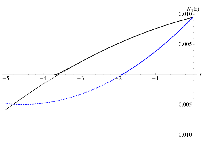
Figure 1: Lower (blue) line is for $\gamma=1/4$ and upper (black) line is for $\gamma=0$. Dotted lines are the small $-r$ expansion and the solid lines is the exact trace.

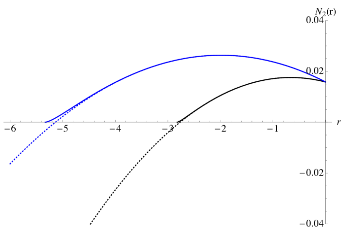
Figure 2: Upper (blue) line is for $\alpha=-1/6$ and lower (black) line is for $\alpha=0$. Dotted lines are the small $-r$ expansion and the solid lines is the exact trace.

2.7 Expansion around the critical values

It is interesting to see the $x\to 0$ limit of the integrals $I_{n}(x)$ defined by (2.31) corresponding to the IR limit. In this limit, we find

$$I_{1}(x) \approx \frac{\pi x^{3}}{3}\Big{(}1-\frac{(\pi x)^{2}}{5}+\frac{2}{35}(\pi x)^{4}+\cdots\Big{)},$$

$$I_{3}(x) \approx \frac{\pi x^{5}}{5}\Big{(}1-\frac{5}{21}(\pi x)^{2}+\frac{2}{27}(\pi x)^{4}+\cdots\Big{)},$$

$$I_{5}(x) \approx \frac{\pi x^{7}}{7}\Big{(}1-\frac{7}{27}(\pi x)^{2}+\frac{14}{165}(\pi x)^{4}+\cdots\Big{)}.$$ (2.39)

This approximation is valid when the curvature is close to the boundary of the range (2.28), and it appears that we get non-analytic behaviour due to the square roots in (2.26). However this non-analyticity does not lead to a complex flow equation since (2.39) is used only in the range of $r$ (2.28) where the square root is real, and the term vanishes beyond the range. A consequence of the non-analytic behaviour will be that the solution to the fixed point equation will generically be non-analytic around the points where $r=r_{{\rm crit},j}$ for which $x=0$. Similar behaviour is observed for the odd dimensional case, where the integrals does not involve arctangent so that they give exact polynomials. This can be seen in the the exact expression for $d=3$ given in appendix C.

We note that the expansions (2.39) correspond to asymptotically large negative $r$ for the choice of endomorphism (2.29) whereby the range (2.28) extends to $r=-\infty$, and the large $r$ corresponds to small $x$.

3 Polynomial solutions in four dimensions

We now analyse the FP solutions $\dot{\varphi}=0$ of the flow equation for $d=4$ in the small $|r|$ approximation (2.38). As we have noted, the flow equation then takes a similar form to that of the equation on a sphere using the heat kernel expansion. The differences arise from the difference in the treatment of some modes in the heat kernel expansions for different topologies. In addition, since we know the exact equation we can better assess the approximation being made.

3.1 Einstein-Hilbert at one-loop

It is well known that pure gravity with the Einstein-Hilbert action is renormalizable on shell at one-loop. Furthermore it is found that there is a UV FP within this approximation when we ignore higher order curvature terms and truncate the theory to just the Einstein-Hilbert action. It is interesting therefore to see what is modified if we do not neglect the higher order curvature terms which are present in the $f(R)$ approximation. An important point is that one-loop renormalization in Einstein theory relies on the fact that the Gauss-Bonnet term $\int d^{4}xE\;[\,\equiv\int d^{4}x\,(R_{\mu\nu\rho\lambda}^{2}-4R_{\mu\nu}^{2}+R^{2})]$ is a topological invariant. On a constant curvature spacetime, we have that $\int d^{4}xE\propto\int d^{4}xR^{2}$ and hence we can neglect terms which are of order $R^{2}$ in the flow equation by including, in addition to the Einstein-Hilbert action, also the Gauss-Bonnet term. We therefore look for a FP solution to the one-loop $f(R)$ flow equation (i.e. where $\eta=0$) with

$$\varphi(r)=g_{0}+g_{1}r,$$ (3.1)

inserted on the RHS of the one-loop equation and with an additional term $-\frac{r^{2}}{\sigma}$ which appears only on the LHS originating from the topological invariant. The couplings $g_{0}=\lambda/(8\pi g)$ and $g_{1}=-1/(16\pi g)$ are then related to the dimensionless Newton’s coupling $g=k^{2}G$ and cosmological constant $\lambda=k^{-2}\Lambda$ which form the dimensionless product $G\Lambda=g\lambda$. It is evident that such a solution, containing only two dynamical couplings, cannot be global. However if we use the asymptotic approximation (2.38), we can still hope that no terms outside Einstein-Hilbert truncation are renormalized in the small curvature limit. In this limit one finds

$$4g_{0}+2rg_{1}+\beta_{\sigma}r^{2}/\sigma^{2}=\frac{\frac{1}{2}r\left(900\alpha-540\gamma-\frac{905r}{6\alpha r+r+6}-\frac{158r}{4\gamma r-r+4}-675\right)+180}{2880\pi^{2}},$$ (3.2)

where we are looking for a FP for $g_{0}$ and $g_{1}$. One observes that for general $\alpha$ and $\gamma$, there is no solution if we require that this be valid for arbitrary $r$. Instead one is forced to set $\alpha=-1/6$ and $\gamma=1/4$ such that the RHS is quadratic in $r$. Then we obtain the FP

$$g_{0}=\frac{1}{64\pi^{2}}\,,\,\,\,\,\,\,g_{1}=-\frac{1}{12\pi^{2}}\,.$$ (3.3)

Additionally one finds that

$$\beta_{\sigma}=-\frac{571}{45}\frac{1}{384\pi^{2}}\sigma^{2},$$ (3.4)

which is actually a universal result independent of the regulator function and endomorphisms as can be confirmed by comparison with the well known one-loop analysis [47]. Here observe that the requirement that there be no nonzero irrelevant couplings in the small curvature limit actually specifies the values of the endomorphisms. The same can be said of the shape function since it is only by using the optimised cutoff that the regulated Hessians can become constants independent of $\bar{R}$. This singles out this choice of regulator up to rescaling of the cutoff scale which keeps the dimensionless product

$$g_{*}\lambda_{*}=\frac{9\pi}{128},$$ (3.5)

invariant. Given that we have an exact scaling solution in the limit $-r\to 0$, we could in principle use this information to set the boundary condition and integrate the FP equation towards $r\to-\infty$ in order to probe effects at large curvature. Here we will instead look for solutions involving dynamical higher order terms beyond the one-loop approximation.

3.2 Quadratic solutions

Exploiting the small curvature approximation, it is possible to look for quadratic solutions where the $r^{2}$ term is dynamical. Following [18], we look for such solutions for values of $\alpha,\beta$ and $\gamma$ determined by requiring $\varphi(r)$ is quadratic.

They are obtained by plugging into the FP equation for small $r$ approximation the ansatz

$$\varphi(r)=g_{0}+g_{1}r+g_{2}r^{2},$$ (3.6)

and writing the equation as $\frac{N}{D}=0$. Here $N$ is a polynomial of fifth order in $r$ and $N=0$ can be solved for the six unknowns $\alpha,\beta,\gamma,g_{0},g_{1}$ and $g_{2}$. Since we are making a small $r$ approximation, we know that these solutions cannot in fact be global but can give quite good approximation to the exact solutions. Of course for the solution to be consistent with the exact equation, the bounds (2.16) must be satisfied.

We then find the following distinct solutions listed in Table 1 where the critical exponents have been found using polynomial expansions around $r=0$ up to order $n$ as indicted. Only 6th and 7th solutions have stable critical exponents $\theta$ less than or equal to 4 and are reliable. Both have three relevant critical exponents. The third one appears to have critical exponents less than or equal to 4, but they are not stable and not reliable.

$\alpha$	$\beta$	$\gamma$	$10^{3}g_{0}$	$10^{3}g_{1}$	$10^{3}g_{2}$	$\theta\;(n=7)$	$\theta\;(n=8)$	$\theta\;(n=9)$
$-0.441$	$-0.0460$	$-0.129$	9.42	$-3.80$	0.721	0.389	3.24	433, 0.776
$-0.463$	$-0.0468$	$-0.0468$	9.33	$-4.62$	0.877	0.301	1.73	153, 0.783
0.767	0.250	1.18	5.86	$-2.59$	0.589	0.604	$3.54,0.706$	0.359
1.85	3.09	2.27	3.42	$8.97$	2.84	8.02	7.80	7.54
0.805	0.308	$-0.238$	5.40	$5.23$	$-1.28$	7.29	$8.47\pm 2.47i$	7.08
$-0.497$	$-4.22$	$0.278$	$2.96$	$-16.6$	$-0.235$	2.94, 0.980	2.94, 0.982	2.94, 0.984
$-0.266$	$-17.8$	$0.252$	$2.91$	$-12.7$	$-0.0119$	2.76, 1.75	2.76, 1.74	2.76, 1.74
$-0.683$	$-0.102$	$-0.165$	6.92	$-9.63$	2.00	12.0, 5.30	$0.00326,12.6\pm 17.5i$	8.92
$-1.13$	$-0.432$	$-0.354$	4.67	$-17.8$	5.38	$6.29\pm 1.48i$	$6.07\pm 0.68i$	9.68, 4.12
2.21	3.24	1.17	3.48	$18.7$	8.56	$4.09$	$4.05$	4.00

Table 1: Quadratic solutions of the spectral sum FP equation. In the last column, we report the results for the positive (real part of) critical exponents, evaluated up to 9th order polynomial expansion. The critical exponent $4$ is present in all solutions and is related to the cosmological term. Those solutions with critical exponents larger than 4 are not reliable.

Unfortunately, the bounds Eq. (2.16) on $\alpha$ and $\beta$ are violated for the sixth FP as is the bound on $\beta$ for the seventh FP. As a consequence these solutions do not make sense globally even if we were to integrate towards larger curvature.

3.3 Polynomial solutions

We next study polynomial solutions to the flow equation which can be compared with those obtained on compact spacetimes. To this end, we look for solutions of the form:

$$\varphi_{p}(r)=\sum_{i=0}^{n}g_{i}r^{i},$$ (3.7)

for fixed endomorphism parameters $\alpha,\beta$ and $\gamma$. In particular we take the case where the reference operator is $-\bar{\nabla}^{2}$ for all modes, and a type-II cutoff where the reference operator contains precisely the $\bar{R}$-terms that are present in the Hessian. In addition we also present solutions for the choice (2.29). For each of these cases, we have looked for convergence of the couplings and critical exponents as the order $n$ is increased. Unlike the case for the compact spacetime [9, 14, 18, 19], we do not find good convergence of the values of the couplings or critical exponents from order to order. An interesting observation, though, is that the coefficients for higher order terms than quadratic are in general very small. For example, using the type I cutoff we have at order $n=8$ solutions

$$\varphi_{p}(r) = 0.00346-0.00940r-0.00371r^{2}+5.96\times 10^{-5}r^{3}+3.19\times 10^{-4}r^{4}$$ (3.8)

$$+2.67\times 10^{-5}r^{5}-1.71\times 10^{-5}r^{6}-8.46\times 10^{-8}r^{7}+\cdots,$$

with the three relevant eigenvalues of the stability matrix $-41.5$, $-4$, $-1.69$ and

$$\varphi_{p}(r) = 0.00389-0.00197r+0.00168r^{2}-2.84\times 10^{-4}r^{3}-8.44\times 10^{-5}r^{4}$$ (3.9)

$$-7.80\times 10^{-6}r^{5}-1.15\times 10^{-5}r^{6}-1.01\times 10^{-6}r^{7}+\cdots,$$

with just two relevant eigenvalues $-4$, $-0.825$. Extending the order to $n=9$, we then find solutions

$$\varphi_{p}(r) = 0.00397-0.00373r+0.00241r^{2}-8.74\times 10^{-5}r^{3}-1.46\times 10^{-4}r^{4}$$

$$-1.43\times 10^{-5}r^{5}-1.38\times 10^{-5}r^{6}-1.05\times 10^{-5}r^{7}+\cdots,$$

$$\varphi_{p}(r) = 0.00331-0.00872r-0.00157r^{2}+0.00151r^{3}+0.000591r^{4}$$

$$+0.0000737r^{5}+0.000106r^{6}+0.0000746r^{7}+0.0000225r^{8}+0.0000126r^{9},$$

$$\varphi_{p}(r) = 0.00254-0.00971r+0.000508r^{2}+0.000425r^{3}-0.000833r^{4}$$ (3.10)

$$+0.00160r^{5}-0.0116r^{6}-0.0293r^{7}-0.000213r^{8}+0.0546r^{9}.$$

The relevant eigenvalues have real parts given by $-21.21$, $-21.21$, $-4$, $-1.46$ for the first FP, $-4.85377$, $-4$, $-2.02686$ for the second FP and $-4,-3.57868,-3.57868,-3.42532,-2.50629$ for the third FP. When there are two same eigenvalues, this means that they are a complex conjugate pair and we show just the real parts.

Using a type II cutoff with $\alpha=-\frac{1}{6}$, $\beta=\frac{1}{3}$ and $\gamma=\frac{1}{4}$, we find for $n=8$ the fixed points

$$\varphi_{p}(r) = 0.00343-0.0120r-0.00390r^{2}+5.20\times 10^{-5}r^{3}+2.93\times 10^{-4}r^{4}$$ (3.11)

$$+2.71\times 10^{-5}r^{5}-3.10\times 10^{-5}r^{6}-3.46\times 10^{-6}r^{7}+\cdots,$$

with the three relevant eigenvalues $-13.3$, $-4$, $-1.65$, and

$$\varphi_{p}(r) = 0.00398-0.00727r+0.00454r^{2}+6.63\times 10^{-4}r^{3}-1.66\times 10^{-4}r^{4}$$ (3.12)

$$-2.75\times 10^{-5}r^{5}+2.48\times 10^{-5}r^{6}-2.63\times 10^{-5}r^{7}+\cdots,$$

with the eigenvalues $-9.97$, $-4$, $-2.06$.

Using the cutoff with (2.29) $\alpha=-\frac{17}{48}$, $\beta=-\frac{9}{48}$, $\gamma=-\frac{13}{48}$, we find for $n=8$

$$\varphi_{p}(r) = 0.003310-0.01206r-0.002131r^{2}+5.210\times 10^{-4}r^{3}+5.697\times 10^{-4}r^{4}$$

$$+2.109\times 10^{-4}r^{5}+3.899\times 10^{-5}r^{6}+1.700\times 10^{-6}r^{7}+5.435\times 10^{-6}r^{8},$$

$$\varphi_{p}(r) = 0.003273-0.01205r-0.001767r^{2}+8.960\times 10^{-4}r^{3}+7.664\times 10^{-4}r^{4}$$

$$+2.830\times 10^{-4}r^{5}+8.320\times 10^{-5}r^{6}+2.885\times 10^{-6}r^{7}+2.814\times 10^{-5}r^{8},$$

$$\varphi_{p}(r) = 0.003237-0.01215r-0.001483r^{2}+0.001351r^{3}+0.001503r^{4}$$ (3.13)

$$+2.831\times 10^{-4}r^{5}+8.360\times 10^{-4}r^{6}-1.618\times 10^{-4}r^{7}+6.824\times 10^{-4}r^{8}\,,$$

with the negative eigenvalues for the stability matrix $-3.98$, $-4$ for the fist solution, and $-4.09$, $-4$, $-1.05$ for the second and $-4$, $-3.05$, $-1.33$, $-1.33$ for the third.

For $n=9$, we find the fixed points

$$\varphi_{p}(r) = 0.003341-0.01214r-0.002510r^{2}+2.181\times 10^{-4}r^{3}+0.0004578r^{4}+1.983\times 10^{-4}r^{5}$$

$$+3.688\times 10^{-5}r^{6}-1.275\times 10^{-6}r^{7}-1.430\times 10^{-6}r^{8}+2.486\times 10^{-6}r^{9},$$

$$\varphi_{p}(r) = 0.003413-0.01259r-0.003815r^{2}-7.380\times 10^{-4}r^{3}+1.469\times 10^{-4}r^{4}$$

$$+2.142\times 10^{-4}r^{5}+1.004\times 10^{-4}r^{6}+1.489\times 10^{-5}r^{7}-8.428\times 10^{-6}r^{8}-9.574\times 10^{-6}r^{9},$$

$$\varphi_{p}(r) = 0.003196-0.01241r-0.001220r^{2}+0.001926r^{3}+0.008472r^{4}-8.934\times 10^{-4}r^{5}$$

$$+0.01177r^{6}+0.01908r^{7}-0.01366r^{8}+0.1067r^{9},$$

$$\varphi_{p}(r) = 0.003253-0.01210r-0.001601r^{2}+0.001169r^{3}+9.672\times 10^{-4}r^{4}+4.247\times 10^{-4}r^{5}$$ (3.14)

$$+1.662\times 10^{-4}r^{6}+1.238\times 10^{-4}r^{7}+7.082\times 10^{-5}r^{8}+5.341\times 10^{-5}r^{9},$$

with the negative eigenvalues for the stability matrix $-4$, $-3.14$ for the first solution, $-9.00$, $-4$, $-1.16$ for the second $-4$, $-3.07$, $-0.33$, $-0.33$ for the third and $-5.27$, $-4$, $-2.18$ for the fourth fixed point, respectively.

In all these cutoff schemes, the number of relevant directions varies from two to five, and the degree of convergence of the solutions for the hyperbolic case seem to be poorer compared with the compact case when we increase the number of the polynomial terms, though some of them look to have better convergence. This makes a sharp contrast to the polynomial solutions for compact spaces studied before [6, 7, 8, 9, 48, 18, 19]. However we cannot rule out the possibility that convergence will be found at orders beyond those considered here.

4 Global solutions in four dimensions

We now turn our attention to global solutions to the flow equation in four dimensions.

4.1 Asymptotically free solutions

First we will look for solutions to the flow equation where the $R^{2}$ coupling is allowed to diverge. In this way we can consider asymptotically free fixed points without truncating the $f(R)$ action.

To begin with, we consider the fixed point equation with $\dot{\varphi}(r)=0$ and where we allow the $r^{2}$ coupling to diverge. To find the solution, we write

$$\varphi(r)=-\frac{r^{2}}{b}+\phi(r),$$ (4.1)

and insert this ansatz into the fixed point equation. We are interested in solving the fixed point equation for $b\to 0$ to obtain a finite part $\phi(r)$. To this end, we expand the equation in $b$ and it then takes the simple form:

$$4\phi(r)-2r\phi^{\prime}(r)=\frac{N_{2}(r)\Theta\left(r+\frac{1}{\alpha+\frac{17}{48}}\right)}{\alpha r+\frac{r}{6}+1}+\frac{N_{0}(r)\Theta\left(r+\frac{1}{\beta+\frac{3}{16}}\right)}{\beta r+1}-\frac{N_{1}(r)\Theta\left(r+\frac{1}{\gamma+\frac{13}{48}}\right)}{(\gamma-\frac{1}{4})r+1}+\mathcal{O}(b).$$ (4.2)

where we include the theta functions to make explicit the vanishing of the traces at the critical values of curvature (2.28). Since the RHS of (4.2) is independent of $\phi(r)$, the equation can be integrated straightforwardly. We observe that there are poles depending on the endomorphism parameters which in principle can lead to a break down of the convexity of the effective action. To remove them, we put $\alpha=-1/6$, $\beta=0$ and $\gamma=1/4$ which set all the denominators to $1$. The contribution of the spin one degree of freedom then vanishes at $r=-48/25$ whereas the spin zero and spin two contributions vanish at $r=-16/3$. We can then solve this equation (4.2) in the small $r$ regime, obtaining

$$\phi(r)=\frac{1}{2}\frac{371r^{2}\log(r^{2})}{23040\pi^{2}}-\frac{5r}{64\pi^{2}}+\frac{3}{128\pi^{2}}+ar^{2},$$ (4.3)

where $a$ is an integration constant. We note that the coefficient of the $r^{2}\log(r^{2})$ can be shown to be universal i.e. independent of the choice of the endomorphisms and the cutoff function. For a different choice of the endomorphism parameters, we would obtain additional terms $\sim r^{2}\log((4\gamma-1)r+4)$, $\sim r^{2}\log(6\alpha r+r+6)$ and $\sim r^{2}\log(\beta r+1)$ as well as modified coefficients for the constant and linear terms. The solution (4.3) can be analytically continued to positive curvature provided the curvature is smaller than the radius on convergence $|r|<r_{C}$ for the small curvature expansion.

In the small $r$ approximation, we can look for constant curvature solutions $r=r_{0}$ to the equation of motion (2.3) for either sign which in the dimensionless form corresponds to $4\phi(r_{0})-2r_{0}\phi^{\prime}(r_{0})=0$. We note that the $r^{2}$ term in $\varphi$ does not alter the equation of motion. We then find a pair of solutions to this equation of motion at positive and negative curvatures:

$$r_{+}=\frac{6}{371}\left(\sqrt{33630}-150\right)\approx 0.539917\,,\,\,\,\,\,\,\,r_{-}=\frac{6}{371}\left(-150-\sqrt{33630}\right)\approx-5.39167.$$ (4.4)

To determine whether $r_{+}$ is a physical solution, we need to verify that $r_{+}<r_{C}$ where $r_{C}$ is the value of $|r|$ for which the small $r$ approximation breaks down. To check whether $r_{-}$ is physical, we look at the exact form of (4.2).

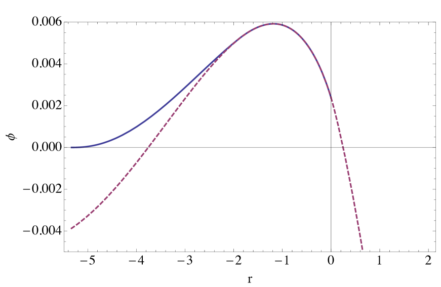
Figure 3: Global solution for negative curvature with an asymptotically free $r^{2}$ coupling. Boundary conditions are set so that $\phi(-16/3)=0$, for the exact solution, fixing the finite $r^{2}$ contribution. The solid (blue) line is the exact solution whereas the dashed (purple) line is the small curvature approximation which is continued for positive curvature. We note that the vanishing of the solution for $r=-16/3$ is imposed by choosing the constant of integration $a$ suitably.

To study this, let us first obtain the global solution for $-\infty<r<0$ by integrating (4.2). The plot of the obtained solution is shown in Fig. 3 and compared to the small $r$ approximation. We observe that the small curvature approximation is in agreement up till the point where the first theta function vanishes at $r=-48/25$. As such, an estimate for the radius of convergence of the small $r$ expansion is obtained as

$$r_{C}\approx 48/25\,,$$ (4.5)

which indicates that the positive solution in (4.4) is well within the radius of convergence.

What about $r_{-}$? The absolute value $|r_{-}|$ is outside of this, and this is a first indication that it may not be a physical solution. Since the RHS of (4.2) is zero at $r=-16/3$, it follows that the solution beyond this point is simply of $r^{2}$ form. Furthermore due to this vanishing, we have a solution to the equation of motion at this point:

$$r_{-}=-16/3\approx-5.33333,$$ (4.6)

which is in good agreement with $r_{-}$ in the small curvature approximation (4.4). The value $4\phi-2r\phi^{\prime}$ of the equation of motion is plotted in Fig. 4 which is found simply by plotting the RHS of (4.2). The existence of this solution is due to the fact that the RHS of the flow equation vanishes once the last modes is integrated out. When at least one parameter takes its critical value (2.29), the RHS never vanishes for the whole finite range of negative $r$, and only the $r_{-}=-\infty$ can be a solution. This means that $r_{-}$ is not generically finite. We take this as a second evidence that it is not physical.

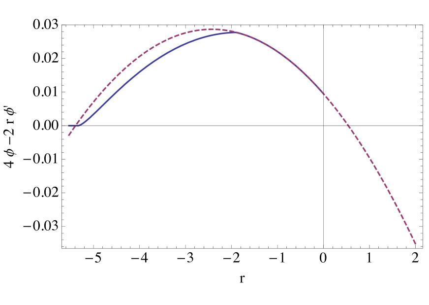
Figure 4: The equation of motion for the asymptotically free fixed point. The solid (blue) line is the exact result whereas the dashed (purple) line is the small curvature approximation. We observe that up to the point where the first theta functions vanish, the small $r$ approximation is in excellent agreement with the exact result. There are solutions for both positive and negative curvatures. However the latter can be considered as an artifact of the optimised cutoff.

It is important to realize that the fixed point solution $\phi(r)$ with a free $r^{2}$ coupling is not the most general solution to the flow equation found in the limit of $b\to 0$. In fact we have implicitly assumed that

$$\partial_{t}\frac{1}{b}=0,$$ (4.7)

to obtain $(\ref{AfreeFP})$ which follows from $\dot{\varphi}=0$. In this sense the solution is a true fixed point. However when we expand $\phi(r)$ for small $r$, we will obtain a non-analytic expression due to the $r^{2}\log(r^{2})$ term in (4.3). This suggests the existence of a different solution to the flow equation without a strict scaling solution condition ($\dot{\varphi}=0$). Instead, we look for a solution with the beta function for the $R^{2}$ couplings

$$\beta_{b}\equiv\partial_{t}b=-wb^{2}+\mathcal{O}(b^{3}),$$ (4.8)

where we assume $w\neq 0$. Such a fixed point obtained in the $f(R)$ approximation can be understood as an approximation to the well-known asymptotically free fixed point in curvature squared gravity [49, 50, 51, 3, 4]. Here since we include only the $R^{2}$ term, we will only get an approximation to the full theory. A similar approximation has been considered in [52] where only the $R$ and $R^{2}$ terms were retained revealing an asymptotically free fixed point. Here we are not limited by the small curvature expansion and can therefore find a more general solution of the $f(R)$ type. To this end, we write an ansatz for this solution as

$$\varphi(r)=-\frac{r^{2}}{b}+\tilde{\phi}(r),$$ (4.9)

where for small $b$ we further demand that $\partial_{t}b=\beta_{b}$ be given by (4.8). Inserting this ansatz into the flow equation with $\partial_{t}\tilde{\phi}(r)=0$ and again taking the limit $b\to 0$, the flow equation then takes the form

$$4\tilde{\phi}(r)-2r\tilde{\phi}^{\prime}(r)-wr^{2}=\frac{N_{2}(r)\Theta\left(r+\frac{1}{\alpha+\frac{17}{48}}\right)}{\alpha r+\frac{r}{6}+1}+\frac{N_{0}(r)\Theta\left(r+\frac{1}{\beta+\frac{3}{16}}\right)}{\beta r+1}-\frac{N_{1}(r)\Theta\left(r+\frac{1}{\gamma+\frac{13}{48}}\right)}{(\gamma-\frac{1}{4})r+1}+\mathcal{O}(b)\,,$$ (4.10)

for small $b$. To determine $w$, we now demand that $\tilde{\phi}(r)$ be analytic in the limit $r\to 0$ which means that for small curvature, $\tilde{\phi}(r)$ has a polynomial expansion

$$\tilde{\phi}(r)\sim\sum_{n}\tilde{g}_{n}r^{n},$$ (4.11)

for finite coefficients $\tilde{g}_{n}$. Expanding (4.10) for small $r$, we then have

$$4g_{0}+2g_{1}r-r^{2}w+\cdots=\frac{3}{32\pi^{2}}+\frac{(60\alpha+12\beta-36\gamma-41)}{384\pi^{2}}r-\frac{371}{11520\pi^{2}}r^{2}+\cdots.$$ (4.12)

It follows that the coefficient of the universal $r^{2}$ term determines the value of the coefficient appearing in (4.8) to be

$$w=\frac{371}{11520\pi^{2}},$$ (4.13)

independently of $\alpha$, $\beta$ or $\gamma$. This differs from the coefficient $\frac{1117}{8640\pi^{2}}$ found in [52] where the equation was evaluated on a sphere. We then observe that $b$ is asymptotically free coupling which behaves as

$$\frac{1}{b}=\frac{371\log(k^{2}/\mu^{2})}{23040\pi^{2}}.$$ (4.14)

Setting $\alpha=-1/6$, $\beta=0$ and $\gamma=1/4$, we remove the other non-analytic terms as before. Now we have the solution (4.11) for small $r$ given by

$$\tilde{\phi}(r)=\frac{3}{128\pi^{2}}-\frac{5r}{64\pi^{2}}+ar^{2},$$ (4.15)

without the logarithmic term. In fact the solution $\tilde{\phi}(r)$ is related to the the solution $\phi(r)$ by

$$\tilde{\phi}(r)=\phi(r)-\frac{1}{2}\frac{371r^{2}\log(r^{2})}{23040\pi^{2}},$$ (4.16)

for all $r$ since both (4.2) and (4.10) are linear differential equations which differ only by the term $-wr^{2}$. Here the additional term is expected to be universal since it carries the coefficient of the logarithmic divergence.

We can look again for constant curvature solutions to the equation of motion (2.3) which are then solutions to $4\tilde{\phi}(r_{0})-2r_{0}\tilde{\phi}^{\prime}(r_{0})=0$ which receive an extra term $wr^{2}$ compared to the equation of motion for $\phi$. In the small $r$ approximation, using (4.15), we have

$$4\tilde{\phi}(r)-2r\tilde{\phi}^{\prime}(r)\approx\frac{3}{32\pi^{2}}-\frac{5r}{32\pi^{2}},$$ (4.17)

which now only has a solution for positive curvature $r_{0}=3/5$. In Fig. 5 we plot the exact form of $4\tilde{\phi}(r)-2r\tilde{\phi}^{\prime}(r)$ observing that there is no solution for negative curvature. To check the stability of the de-sitter solution at $r_{0}=3/5$, we can compute the mass of the scalaron $m$ by evaluating $m^{2}\equiv U^{\prime\prime}(\phi_{0})$ given by (2.15) at the minimum corresponding to $R_{0}=\frac{3}{5}k^{2}$. The stability of de-Sitter space requires $m^{2}>0$. Explicitly we find

$$\frac{m^{2}}{k^{2}}\equiv\frac{1}{k^{2}}\frac{1}{3f^{\prime\prime}(R_{0})}(f^{\prime}(R_{0})-R_{0}f^{\prime\prime}(R_{0}))=\frac{5}{384\pi^{2}}\frac{23040\pi^{2}}{371\log(k^{2}/\mu^{2})},$$ (4.18)

where the subleading dependence on $a$ is neglected. This is positive in the UV limit as a consequence of $w>0$. Additionally we have $f^{\prime}(R_{0})<0$ which is also needed for the graviton to have the right sign kinetic term.

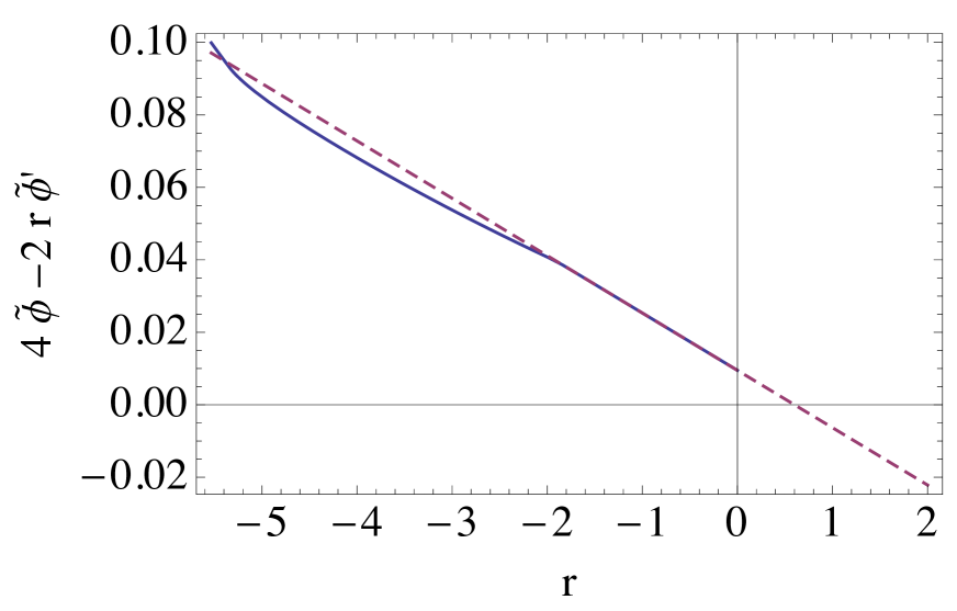
Figure 5: The equation of motion for the asymptotically free fixed point approached with the $R^{2}$ coupling is governed by (4.8) with the universal coefficient (4.13). While there are no solutions for negative curvature the analytical continuation of the small $r$ approximation (dashed line) reveals a solution at positive curvature $r_{0}=3/5$.

Lowering the cutoff scale such that $R/k^{2}<-16/3$, the RHS of the flow equation vanishes and we then obtain the effective action:

$$\int d^{4}x\sqrt{g}f(R)=\int d^{4}x\sqrt{g}\left(aR^{2}-\frac{371R^{2}\log(R^{2}/\mu^{4})}{46080\pi^{2}}\right),$$ (4.19)

where the $k$-dependence has cancelled between the $R^{2}/b$ term and the $R^{2}\log(R^{2}/k^{4})$ term. Here we can take $a$ as a free parameter and fix $\mu$ to some fixed reference scale. We conclude that in the UV, the solution is asymptotically free with a coefficient (4.13) and that in the IR, the action stops running to take the form (4.19). Thus we have an effective action obtained after all quantum corrections have been integrated out.

Since the fixed point here is perturbative, it is straightforward to find the critical exponents. Adding a scale-dependent perturbation to the solution $\tilde{\phi}+e^{t\theta}\delta\varphi(r)$, one finds that the perturbations are simply solutions to

$$\theta\delta\varphi(r)+4\delta\varphi(r)-2r\delta\varphi^{\prime}(r)=0,$$ (4.20)

and thus the only analytic solutions are integer powers of $\delta\varphi(r)\propto r^{n}$ with the eigen-spectrum

$$\theta=-4+2n\,.$$ (4.21)

Hence in addition to the asymptotically free $R^{2}$ coupling, there are two further relevant couplings corresponding to the vacuum energy and Newton’s constant. The requirement of asymptotic safety then demands that we set all irrelevant perturbations to zero, while the relevant perturbations generate an Einstein-Hilbert action which we can add to (4.19) to obtain the effective action

$$\int d^{4}x\sqrt{g}f(R)=\int d^{4}x\left(\frac{1}{16\pi G}(-R+2\Lambda)+aR^{2}-\frac{371R^{2}\log(R^{2}/M_{Pl}^{4})}{46080\pi^{2}}\right)\,.$$ (4.22)

Here we have fixed the reference scale to the Planck mass $\mu=M_{Pl}\equiv 1/\sqrt{G}$ without loss of generality. We then have three free parameters $a$, $G$ and $\Lambda$. This effective action (with $\Lambda=0$ and $f\to-f$ after rotation to Lorentzian signature) has been studied in [53] in the context of inflation and gives rise to a hilltop inflation.

4.2 Global numerical solutions

We can also analyse the flow equation given in Eq. (2.32) at fixed endomorphisms, and search for global numerical solutions with finite couplings. For this purpose, it is convenient to choose the parameters (2.29) such that the RHS of the flow equation is nonzero over the whole range $-\infty<r<0$ without singularities. The flow equation then takes the same form for the whole range of $r<0$, and we can try to study the asymptotic expansion for large $r$ using (2.39). The expansion takes the form

$$\varphi(r) = ar^{2}+\sum_{n=1}^{\infty}a_{i}(a)\frac{1}{(-r)^{i/2}}\,,$$ (4.23)

where $a$ is an arbitrary number. Explicitly we find

$$\varphi(r) = ar^{2}+\frac{323}{1500\pi}\frac{\sqrt{3}}{(-r)^{1/2}}-\frac{26648+14535\pi^{2}}{39375\pi}\frac{\sqrt{3}}{(-r)^{3/2}}$$ (4.24)

$$+\frac{8(9181648+3975660\pi^{2}+3270375\pi^{4})}{26578125\pi}\frac{\sqrt{3}}{(-r)^{5/2}}+\cdots\,.$$

At higher orders in the asymptotic expansion, one finds that the coefficients of $a_{i}$ become dependent on $a$ as indicated in (4.23). The large negative curvature expansion therefore gives a one parameter family of solutions in the asymptotic limit.

As a consequence of the asymptotic behaviour, global solutions are reduced to a one parameter family despite the equation being third order. By numerically integrating the fixed point equation starting at large $-r$ we can then give initial conditions for different values of $a$ matching the asymptotic expansion. Furthermore at $r=0$, we have to impose a regularity condition which removes the remaining one free parameter since we then need to tune $a$. For finite $r$, there are no further fixed singularities which would otherwise over constrain the equation. As a result, we expect at most a discrete number of regular global solutions, at least for the choice (2.29).

We have not been able to manage to find any global solutions of this type numerically. However, a full numerical study is beyond the scope of this paper and we cannot rule out there existence. This is left for future study.

5 Summary and discussions

In this paper we have derived a nonperturbative flow equation for quantum gravity on hyperbolic spacetimes of constant curvature. The equation assumes that the scale-dependent effective action is of the $f(R)$ form and hence is not sensitive to tensor structures which fall outside of this approximation. While such tensor structures are irrelevant on the LHS of the flow equation for maximally symmetric spacetimes, curvature squared terms will alter the form of the flow equation since they contribute to $\Gamma^{(2)}_{k}$.

Although the flow equations for $f(R)$ gravity have been studied previously, these were studied on spheres where the traces, evaluated with the optimised cutoff, are discontinuous due to the step functions. Consequently, additional approximations are made to smoothen the flow equation. A key difference for negative curvature spacetimes is that the spectrum of the laplacian is continuous and we therefore do not need to further approximate the traces when using the optimised cutoff. In particular, we observe that once $k^{2}$ is less than the smallest eigenvalue the RHS of the flow equation vanishes indicating the IR limit has been obtained. In this limit we have also noted that the equation becomes non-analytic. One should note that the non-analytic form is the price which is paid for being able to evaluate the traces explicitly with the optimised cutoff.

For small curvature, we have found that the flow equation is well approximated by the equation where the early-time heat kernel expansion is exploited. Here we have found that the flow equations have a quite similar structure to the case of compact spacetimes. Importantly, however, it is clear that this approximation is not applicable globally and breaks down for finite curvature. Nonetheless this approximation is appropriate for studying polynomial solutions around $r=0$. Here another difference from previous equations on the sphere arises since the early-time heat kernel expansion is not modified by the removal of certain modes, as it is on the sphere. It is important to point out that the differences come from the choice of a maximally symmetric background and that it is therefore clear that they will not arise when a generic background is chosen. While these modifications may seem minor, we find that they have a dramatic effect; here we have found rather poor convergence of the polynomial solutions of increasing order. Furthermore, we have observed that the requirement that all modes are integrated out for $k\to 0$ puts a constraint on the form of the differential operator entering the regulator. Therefore the quadratic small curvature solutions which do show convergence (for the eigenvalues) are not permissible since the regulator will not vanish, even in the limit $k\to 0$.

Here we have also studied the flow equation in the case for which the $R^{2}$ coupling is asymptotically free where exact solutions exist. By requiring the analytical behaviour of the solution for $R/k^{2}\to 0$, we find that the beta function for the $R^{2}$ coupling is determined by the universal coefficient. Then by taking $k\to 0$, the effective action is also determined to contain an $R^{2}\log(R^{2})$ type correction. This fixed point can be understood as the projection of the general curvature squared fixed point onto the $R^{2}$ coupling alone. One therefore expects that on a more general backgrounds the effective action will take a more involved form. It is nonetheless pleasing to see how quantum corrections to the effective action are produced in approximations where the form is not truncated to a finite number of terms. It remains to see whether other fixed point solutions may be uncovered to the $f(R)$ flow equation studied here. An analysis of free parameters suggests that there may be at most a discrete number of solutions.

Appendix A Spectrum of Laplacian on hyperbolic space

The curvature tensors satisfy

$$\bar{R}_{\mu\nu\rho\sigma}=\frac{\bar{R}}{d(d-1)}(\bar{g}_{\mu\rho}\bar{g}_{\nu\sigma}-\bar{g}_{\mu\sigma}\bar{g}_{\nu\rho}),~{}~{}~{}\bar{R}_{\mu\nu}=\frac{1}{d}\bar{g}_{\mu\nu}\bar{R},$$ (A.1)

with negative $\bar{R}=-\frac{d(d-1)}{a^{2}}$. The eigenvalues of the Laplacian for spin $j$ on the hyperbolic space $H^{d}$ are continuous and characterized by positive $\lambda$:

$$-\nabla^{2}h^{(\lambda u)}_{\mu_{1}\cdots\mu_{j}}=-\frac{\lambda^{2}+(\frac{d-1}{2})^{2}+j}{d(d-1)}\bar{R}h^{(\lambda u)}_{\mu_{1}\cdots\mu_{j}},$$ (A.2)

where $u$ is the discrete label for distinguishing eigentensors with the same eigenvalues [54]. See also [35]. We note that therefore an operator $-\nabla^{2}-\alpha_{j}\bar{R}$ has a lowest eigenvalue

$$\delta_{j}=-\frac{(\frac{d-1}{2})^{2}+j}{d(d-1)}\bar{R}-\alpha_{j}\bar{R}\,,$$ (A.3)

when $\lambda=0$. Eigentensors $h^{(\lambda u)}_{\mu_{1}\cdots\mu_{j}}$ are normalized as

$$\int_{H^{d}}d^{d}x\sqrt{\bar{g}(x)}h^{(\lambda u)*}\cdot h^{(\lambda^{\prime}u^{\prime})}(x)=\delta_{uu^{\prime}}\delta(\lambda-\lambda^{\prime}).$$ (A.4)

The analogue of the multiplicity for the continuous spectrum is the spectral function, or Plancherel measure, defined by

$$\mu(\lambda)=\frac{\pi\Omega_{d-1}}{2^{d-2}g(j)}\sum_{u}h^{(\lambda u)*}\cdot h^{(\lambda u)}(x),$$ (A.5)

with the volume of $S^{d-1}$

$$\Omega_{d-1}=\frac{2\pi^{d/2}}{\Gamma(d/2)},$$ (A.6)

and the spin factor, the number of independent solutions, given by

$$g(j)=\frac{(2j+d-3)\cdot(j+d-4)!}{(d-3)!\,j!}.$$ (A.7)

[For $d=3$, $g(0)=1$ and $g(j)=2$ for $j\geq 1$.] The spectral function is explicitly given by

$$\mu(\lambda)=\frac{\pi[\lambda^{2}+(j+\frac{d-3}{2})^{2}]}{2^{2(d-2)}\Gamma(d/2)^{2}}\lambda\tanh(\pi\lambda){\prod_{j=1/2}^{(d-5)/2}(\lambda^{2}+j^{2})},$$ (A.8)

for even $d\geq 4$ (for $d=4$ the product is omitted) and

$$\mu(\lambda)=\frac{\pi[\lambda^{2}+(j+\frac{d-3}{2})^{2}]}{2^{2(d-2)}\Gamma(d/2)^{2}}{\prod_{j=0}^{(d-5)/2}(\lambda^{2}+j^{2})},$$ (A.9)

for odd $d\geq 3$.

The trace is given by integrating over the parameter $\lambda$ with the exponent $E_{\lambda}(d,j)$ of the operator $\Delta$ weighted by their multiplicity [35]:

$$\mbox{Tr}_{(j)}[W(\Delta+E)]=\int_{H^{d}}d^{d}x\sqrt{\bar{g}}\,\frac{2^{d-2}g(j)}{\pi\Omega_{d-1}}\Big{(}\frac{-\bar{R}}{d(d-1)}\Big{)}^{d/2}\int_{0}^{\bar{\lambda}^{(j)}}d\lambda\,\mu(\lambda)W(\Delta_{\lambda}+E).$$ (A.10)

where we assume the integrand has support support for $0<\lambda<\bar{\lambda}^{(j)}$.

Appendix B Heat kernel expansions on constant curvature spacetimes

Let $W(-\nabla^{2}-qR)$ be a function of the Laplace type operator such as the ones appearing under the traces of Eq. (2.5). Here we wish to determine the trace over modes of a differentially constrained field in terms of traces for unconstrained fields on constant curvature backgrounds. Here we consider both the non-compact topology $H^{d}$ and the compact topology $S^{d}$. We are interested in the following traces

$${\rm Tr}_{0}^{\prime\prime}\left[W(-\nabla^{2}-\beta R)\right]\,,\,\,\,\,\,{\rm Tr}_{1T}^{\prime}\left[W(-\nabla^{2}-\gamma R)\right]\,,\,\,\,\,\,\,\,\,\,\,{\rm Tr}_{2T^{2}}\left[W(-\nabla^{2}-\alpha R)\right],$$ (B.1)

where ${\rm Tr}_{0}^{\prime\prime}$ denotes the trace over scalar modes with the constant mode and the CKVs removed, ${\rm Tr}_{1T}^{\prime}$ denotes the trace over transverse-vectors with the KVs removed and ${\rm Tr}_{2T^{2}}$ denotes the trace over symmetric transverse-traceless tensors. In particular we are interested in the heat kernel coefficients in four dimensions

$${\rm Tr}_{({\rm spin})}[e^{s(\nabla^{2}+\beta R)}]=\int d^{4}x\sqrt{g}\frac{1}{(4\pi s)^{2}}(b_{0}+b_{2}Rs+b_{4}R^{2}s^{2}+b_{6}R^{3}s^{3}+...),$$ (B.2)

where ${\rm Tr}_{({\rm spin})}$ denotes one of the traces above. The coefficients $b_{n}$ are listed in table 2 where we set $\zeta=1$ on $S^{4}$ and $\zeta=0$ on $H^{4}$. Differences occur because normalisable constant modes, KVs and CKVs exist on the compact topology $S^{d}$ but do not occur on $H^{d}$. Below we account for these differences denoting the number of these modes on the $S^{d}$ ($H^{d}$) by $\Sigma_{\rm const.}=1$ ($\Sigma_{\rm const.}=0$) for the constant modes, $\Sigma_{KV}=\frac{1}{2}d(d+1)$ ($\Sigma_{KV}=0$) for the KVs and $\Sigma_{CKV}=d+1$ ($\Sigma_{CKV}=0$) for the CKVs.

B.1 Scalars

For the scalar trace in (B.1) the difference between the heat kernel coefficients for the two topologies is due to the removal of the constant mode and CKVs from the trace

$${\rm Tr}_{0}^{\prime\prime}\left[W(-\nabla^{2}-\beta R)\right]={\rm Tr}_{0}\left[W(-\nabla^{2}-\beta R)]\right]-\Sigma_{\rm const.}W(-\beta R)-\Sigma_{CKV}W\left(-\beta R+\frac{R}{d-1}\right)\,.$$ (B.3)

The corresponding heat kernel coefficients are given in table 2 on $S^{4}$ ($\zeta=1$) and $H^{4}$ ($\zeta=0$).

B.2 Vectors

First consider a vector $V_{\mu}$ and decompose it as

$$V_{\mu}=V_{\mu}^{T}+\nabla_{\mu}\phi,$$ (B.4)

where $V_{\mu}^{T}$ is a transverse vector. The compete set of eigenmodes of $V_{\mu}$ is then eigenmodes of $V_{\mu}^{T}$ and $V_{\mu}^{L}=\nabla_{\mu}\phi$. From the equation

$$-\nabla^{2}\nabla_{\mu}\phi=\nabla_{\mu}\left(-\nabla^{2}-\frac{R}{d}\right)\phi,$$ (B.5)

we can determine the spectrum of the longitudinal modes from that of a scalar field. However we need to take into account that the constant mode of $\phi$ will not contribute to $V_{\mu}$. It follows that we can express a trace over transverse vectors modes as

$${\rm Tr}_{1T}^{\prime}W(-\nabla^{2}-\gamma R) = {\rm Tr}_{1}W(-\nabla^{2}-\gamma R)-{\rm Tr}_{0}W\left(-\nabla^{2}-\frac{R}{d}-\gamma R\right)$$ (B.6)

$$+\Sigma_{\rm const.}W\left(-\frac{R}{d}-\gamma R\right)-\Sigma_{KV}W\left(\frac{R}{d}-\gamma R\right),$$

where ${\rm Tr}_{1}$ is the trace over unconstrained vectors.

Spin	$b_{0}$	$b_{2}$	$b_{4}$	$b_{6}$
$0$	$1$	$\beta+\frac{1}{6}$	$\frac{1080\beta^{2}+360\beta-540\zeta+29}{2160}$	$\frac{45360\beta^{3}+22680\beta^{2}-68040\beta\zeta+3654\beta+18900\zeta+185}{272160}$
$1T$	$3$	$\frac{1}{4}(12\gamma+1)$	$\frac{2160\gamma^{2}+360\gamma-540\zeta-67}{1440}$	$\frac{181440\gamma^{3}+45360\gamma^{2}-136080\gamma\zeta-16884\gamma+41580\zeta-4321}{362880}$
$2T^{2}$	$5$	$\frac{5}{6}(6\alpha-1)$	$\frac{1}{432}\left(1080\alpha^{2}-360\alpha+270\zeta-271\right)$	$\frac{45360\alpha^{3}-22680\alpha^{2}+34020\alpha\zeta-34146\alpha+7560\zeta-7249}{54432}$

Table 2: Heat kernel coefficients on $H^{4}$ with $\zeta=0$ and $S^{4}$ with $\zeta=1$

B.3 Tensors

Similarly for a tensor, we consider the decomposition

$$h_{\mu\nu}=h^{T}_{\mu\nu}+g_{\mu\nu}\phi+\nabla_{(\mu}V_{\nu)}-\frac{1}{d}g_{\mu\nu}\nabla^{\rho}V_{\rho},$$ (B.7)

where $h^{T}_{\mu\nu}$ is transverse-traceless and the brackets denote the symmetrisation. Then we have the following identity on a constant curvature spacetime:

$$-\nabla^{2}\left(\nabla_{(\mu}V_{\nu)}-\frac{1}{d}g_{\mu\nu}\nabla^{\rho}V_{\rho}\right)=\nabla_{(\mu}\left(-\nabla^{2}-\frac{(d+1)R}{(d-1)d}\right)V_{\nu)}-\frac{1}{d}g_{\mu\nu}\nabla^{\rho}\left(-\nabla^{2}-\frac{(d+1)R}{(d-1)d}\right)V_{\rho},$$ (B.8)

which allows us to express the trace over transverse-traceless modes in terms of a trace of a vector, scalar and tensor. In this case we must remember to remove the KVs and CKVs from the spectrum of $V^{\mu}$. We therefore have the following relation between traces

$${\rm Tr}_{2T^{2}}W(-\nabla^{2}-\alpha R) = {\rm Tr}_{2}W(-\nabla^{2}-\alpha R)-{\rm Tr}_{1}W\Big{(}-\nabla^{2}-\frac{(d+1)R}{(d-1)d}-\alpha R\Big{)}-{\rm Tr}_{0}W(-\nabla^{2}-\alpha R)$$ (B.9)

$$+ \Sigma_{KV}W\Big{(}-\frac{2R}{d(d-1)}-\alpha R\Big{)}+\Sigma_{\rm CKV}W\Big{(}-\frac{R}{d-1}-\alpha R\Big{)},$$

where ${\rm Tr}_{2}$ is the trace over symmetric tensor modes.

Appendix C Spectral sum approach for $d=3$

It may be interesting to study the flow equation for odd dimension since the integrals are simpler. For $H^{3}$, the trace is given by

$${\rm Tr}_{(j)}W(\Delta+E)=\int_{H^{3}}d^{3}x\sqrt{\bar{g}}\,\frac{g(j)}{2\pi^{2}}\Big{(}\frac{-\bar{R}}{6}\Big{)}^{3/2}\int_{0}^{\bar{\lambda}^{(j)}}d\lambda\frac{\pi(\lambda^{2}+j^{2})}{4\Gamma(3/2)^{2}}W(\Delta_{\lambda}+E)\ ,$$ (C.1)

where the eigenvalues and the corresponding multiplicities given in Appendix A are used. The support of $R_{k}(\Delta_{\lambda}(d,j)+E)$ is restricted to the modes:

$$\bar{\lambda}^{(2)}\!=\sqrt{\frac{6}{-r}\!-3-6\alpha}\,,\quad\bar{\lambda}^{(1)}\!=\sqrt{\frac{6}{-r}\!-2-6\gamma}\,,\quad\bar{\lambda}^{(0)}\!=\sqrt{\frac{6}{-r}\!-1-6\beta}\,,\quad$$ (C.2)

The integrals extend up to the these upper bounds.

Using Eq. (C.1) and (2.17), we obtain the following flow equation

$$\dot{\varphi}-2r\varphi^{\prime}+3\varphi$$ (C.3)

$$= \frac{c_{1}(\dot{\varphi}^{\prime}-2r\varphi^{\prime\prime})+c_{2}\varphi^{\prime}}{\varphi^{\prime}[3+(3\alpha+1)r]}+\frac{c_{3}(\dot{\varphi}^{\prime\prime}-2r\varphi^{\prime\prime\prime})+c_{4}\varphi^{\prime\prime}}{2[2+(2\beta-1)r]\varphi^{\prime\prime}+\varphi^{\prime}}-\frac{c_{5}}{3+(3\gamma-1)r},$$

where the coefficients are simply given by

$$c_{1} = \frac{(-r)^{3/2}}{24\sqrt{6}\pi^{2}}\Big{[}\frac{r}{5}(\bar{\lambda}^{(2)})^{5}+2\Big{(}1+\Big{(}\alpha+\frac{7}{6}\Big{)}r\Big{)}(\bar{\lambda}^{(2)})^{3}+24\Big{(}1+\Big{(}\alpha+\frac{1}{2}\Big{)}r\Big{)}\bar{\lambda}^{(2)}\Big{]},$$

$$c_{2} = \frac{(-r)^{3/2}}{24\sqrt{6}\pi^{2}}\Big{[}\frac{r}{5}(\bar{\lambda}^{(2)})^{5}+2\Big{(}3+\Big{(}\alpha+\frac{7}{6}\Big{)}r\Big{)}(\bar{\lambda}^{(2)})^{3}+24\Big{(}3+\Big{(}\alpha+\frac{1}{2}\Big{)}r\Big{)}\bar{\lambda}^{(2)}\Big{]},$$

$$c_{3} = \frac{(-r)^{3/2}}{36\sqrt{6}\pi^{2}}\Big{[}\frac{r}{5}(\bar{\lambda}^{(0)})^{5}+2\Big{(}1+\Big{(}\beta+\frac{1}{6}\Big{)}r\Big{)}(\bar{\lambda}^{(0)})^{3}\Big{]},$$

$$c_{4} = -\frac{(-r)^{3/2}}{36\sqrt{6}\pi^{2}}\Big{[}\frac{r}{5}(\bar{\lambda}^{(0)})^{5}-2\Big{(}1-\Big{(}\beta+\frac{1}{6}\Big{)}r\Big{)}(\bar{\lambda}^{(0)})^{3}\Big{]},$$

$$c_{5} = \frac{(-r)^{3/2}}{6\sqrt{6}\pi^{2}}\Big{[}(\bar{\lambda}^{(1)})^{3}+3\bar{\lambda}^{(1)}\Big{]}.$$ (C.4)

This result is exact and does not involve complicated functions, so that we can easily study the properties of the flow equation. The equation can be compared to the flow equation derived in [34, 55] on a $H^{3}$ and $S^{3}$ in the conformally reduced approximation.

References

- [1] K. S. Stelle, “Renormalization of Higher Derivative Quantum Gravity,” Phys. Rev. D 16 (1977) 953.
- [2] S. Weinberg, “Ultraviolet Divergences In Quantum Theories Of Gravitation,” in Hawking, S.W., Israel, W.: General Relativity (Cambridge University Press), (1980) 790-831.
- [3] A. Codello and R. Percacci, “Fixed points of higher derivative gravity,” Phys. Rev. Lett. 97 (2006) 221301 [hep-th/0607128].
- [4] M. Niedermaier, “Gravitational fixed points and asymptotic safety from perturbation theory,” Nucl. Phys. B 833 (2010) 226.
- [5] O. Lauscher and M. Reuter, “Flow equation of quantum Einstein gravity in a higher derivative truncation,” Phys. Rev. D 66 (2002) 025026 [hep-th/0205062].
- [6] A. Codello, R. Percacci and C. Rahmede, “Ultraviolet properties of -gravity,” Int. J. Mod. Phys. A 23 (2008) 143 [arXiv:0705.1769 [hep-th]].
- [7] P. F. Machado and F. Saueressig, “On the renormalization group flow of -gravity,” Phys. Rev. D 77 (2008) 124045 [arXiv:0712.0445 [hep-th]].
- [8] A. Codello, R. Percacci, C. Rahmede, “Investigating the Ultraviolet Properties of Gravity with a Wilsonian Renormalization Group Equation,” Ann. Phys. 324 (2009) 414 arXiv:0805.2909 [hep-th].
-
[9]
K. Falls, D. Litim, K. Nikolakopulos and C. Rahmede,
“A bootstrap towards asymptotic safety,”
arXiv:1301.4191 [hep-th].
“Further evidence for asymptotic safety of quantum gravity,” Phys. Rev. D 93 (2016) 104022 [arXiv:1410.4815 [hep-th]].
“On de Sitter solutions in asymptotically safe theories,” arXiv:1607.04962 [gr-qc]. - [10] H. Gies, B. Knorr, S. Lippoldt and F. Saueressig, “Gravitational Two-Loop Counterterm Is Asymptotically Safe,” Phys. Rev. Lett. 116 (2016) 211302 [arXiv:1601.01800 [hep-th]].
-
[11]
D. Benedetti, F. Caravelli,
“The Local potential approximation in quantum gravity,”
JHEP 1206 (2012) 017, Erratum-ibid. 1210 (2012) 157
[arXiv:1204.3541 [hep-th]];
D. Benedetti, “On the number of relevant operators in asymptotically safe gravity,” Europhys. Lett. 102 (2013) 20007 [arXiv:1301.4422 [hep-th]]. - [12] J. A. Dietz and T. R. Morris, “Asymptotic safety in the approximation,” JHEP 1301 (2013) 108 [arXiv:1211.0955 [hep-th]].
- [13] J. A. Dietz and T. R. Morris, “Redundant operators in the exact renormalisation group and in the approximation to asymptotic safety,” JHEP 1307 (2013) 064 [arXiv:1306.1223 [hep-th]].
- [14] M. Demmel, F. Saueressig and O. Zanusso, “RG flows of Quantum Einstein Gravity in the linear-geometric approximation ‘’ Annals Phys. 359 (2015) 141 [arXiv:1412.7207 [hep-th]].
- [15] M. Demmel, F. Saueressig and O. Zanusso, “A proper fixed functional for four-dimensional Quantum Einstein Gravity,” JHEP 1508 (2015) 113 [arXiv:1504.07656 [hep-th]].
- [16] R. Percacci and G. P. Vacca, “Search of scaling solutions in scalar-tensor gravity,” Eur. Phys. J. C 75 (2015) 188 [arXiv:1501.00888 [hep-th]].
- [17] P. Labus, R. Percacci and G. P. Vacca, “Asymptotic safety in scalar models coupled to gravity,” Phys. Lett. B 753 (2016) 274 [arXiv:1505.05393 [hep-th]].
- [18] N. Ohta, R. Percacci and G. P. Vacca, “Flow equation for gravity and some of its exact solutions,” Phys. Rev. D 92 (2015) 061501 [arXiv:1507.00968 [hep-th]].
- [19] N. Ohta, R. Percacci and G. P. Vacca, “Renormalization Group Equation and scaling solutions for f(R) gravity in exponential parametrization,” Eur. Phys. J. C 76 (2016) 46 [arXiv:1511.09393 [hep-th]].
- [20] N. Ohta, R. Percacci and A. D. Pereira, “Gauges and functional measures in quantum gravity I: Einstein theory,” JHEP 1606 (2016) 115 [arXiv:1605.00454 [hep-th]].
-
[21]
A. Nink,
“Field Parametrization Dependence in Asymptotically Safe Quantum Gravity,”
Phys. Rev. D 91 (2015) 044030
[arXiv:1410.7816 [hep-th]].
M. Demmel and A. Nink, “Connections and geodesics in the space of metrics,” Phys. Rev. D 92 (2015) no.10, 104013 [arXiv:1506.03809 [gr-qc]]. - [22] D. Benedetti, “Asymptotic safety goes on shell,” New J. Phys. 14 (2012) 015005 [arXiv:1107.3110 [hep-th]].
- [23] G. Narain and R. Percacci, “On the scheme dependence of gravitational beta functions,” Acta Phys. Polon. B 40 (2009) 3439 [arXiv:0910.5390 [hep-th]].
- [24] I. Donkin and J. M. Pawlowski, “The phase diagram of quantum gravity from diffeomorphism-invariant RG-flows,” arXiv:1203.4207 [hep-th].
- [25] N. Ohta and R. Percacci, “Ultraviolet Fixed Points in Conformal Gravity and General Quadratic Theories,” Class. Quant. Grav. 33 (2016) 035001 [arXiv:1506.05526 [hep-th]].
- [26] D. Benedetti, “Essential nature of Newton fs constant in unimodular gravity,” Gen. Rel. Grav. 48 (2016) 68 [arXiv:1511.06560 [hep-th]].
- [27] D. F. Litim and J. M. Pawlowski, “Renormalization group flows for gauge theories in axial gauges,” JHEP 0209 (2002) 049 [hep-th/0203005].
-
[28]
E. Manrique and M. Reuter,
“Bimetric Truncations for Quantum Einstein Gravity and Asymptotic Safety,”
Annals Phys. 325 (2010) 785
[arXiv:0907.2617 [gr-qc]].
E. Manrique, M. Reuter and F. Saueressig, “Matter Induced Bimetric Actions for Gravity,” Annals Phys. 326 (2011) 440 [arXiv:1003.5129 [hep-th]];
“Bimetric Renormalization Group Flows in Quantum Einstein Gravity,” Annals Phys. 326 (2011) 463 [arXiv:1006.0099 [hep-th]]. - [29] D. Becker and M. Reuter, “En route to Background Independence: Broken split-symmetry, and how to restore it with bi-metric average actions,” Annals Phys. 350 (2014) 225 [arXiv:1404.4537 [hep-th]].
- [30] A. Codello, G. D’Odorico and C. Pagani, “Consistent closure of RG flow equations in quantum gravity,” Phys. Rev. D 89 (2014) 081701 [arXiv:1304.4777 [gr-qc]].
- [31] P. Donà, A. Eichhorn and R. Percacci, “Matter matters in asymptotically safe quantum gravity,” Phys. Rev. D 89 (2014) 084035 [arXiv:1311.2898 [hep-th]].
-
[32]
N. Christiansen, B. Knorr, J. Meibohm, J. M. Pawlowski and M. Reichert,
“Local Quantum Gravity,”
Phys. Rev. D 92 (2015), 121501
[arXiv:1506.07016 [hep-th]].
J. Meibohm, J. M. Pawlowski and M. Reichert, “Asymptotic safety of gravity-matter systems,” Phys. Rev. D 93 (2016) 084035 [arXiv:1510.07018 [hep-th]]. - [33] J. A. Dietz and T. R. Morris, “Background independent exact renormalization group for conformally reduced gravity,” JHEP 1504 (2015) 118 [arXiv:1502.07396 [hep-th]].
- [34] M. Demmel, F. Saueressig and O. Zanusso, “RG flows of Quantum Einstein Gravity on maximally symmetric spaces,” JHEP 1406 (2014) 026 [arXiv:1401.5495 [hep-th]].
- [35] D. Benedetti, “Critical behavior in spherical and hyperbolic spaces,” J. Stat. Mech. 1501 (2015) P01002 [arXiv:1403.6712 [cond-mat.stat-mech]].
- [36] D. F. Litim, “Optimized renormalization group flows,” Phys. Rev. D 64 (2001) 105007 [hep-th/0103195].
-
[37]
K. Falls,
“Renormalization of Newton’s constant,”
Phys. Rev. D 92 (2015) 124057
[arXiv:1501.05331 [hep-th]];
“Critical scaling in quantum gravity from the renormalisation group,” arXiv:1503.06233 [hep-th]. - [38] H. W. Hamber, “Scaling Exponents for Lattice Quantum Gravity in Four Dimensions,” Phys. Rev. D 92 (2015) no.6, 064017 [arXiv:1506.07795 [hep-th]].
- [39] T. P. Sotiriou and V. Faraoni, “f(R) Theories Of Gravity,” Rev. Mod. Phys. 82 (2010) 451 [arXiv:0805.1726 [gr-qc]].
- [40] D. Benedetti and F. Guarnieri, “Brans-Dicke theory in the local potential approximation,” New J. Phys. 16 (2014) 053051 [arXiv:1311.1081 [hep-th]].
- [41] M. Hindmarsh and I. D. Saltas, “f(R) Gravity from the renormalisation group,” Phys. Rev. D 86 (2012) 064029 [arXiv:1203.3957 [gr-qc]].
- [42] G. Narain and R. Percacci, “Renormalization Group Flow in Scalar-Tensor Theories. I,” Class. Quant. Grav. 27 (2010) 075001 [arXiv:0911.0386 [hep-th]].
- [43] G. Narain and C. Rahmede, “Renormalization Group Flow in Scalar-Tensor Theories. II,” Class. Quant. Grav. 27 (2010) 075002 [arXiv:0911.0394 [hep-th]].
- [44] T. Henz, J. M. Pawlowski, A. Rodigast and C. Wetterich, “Dilaton Quantum Gravity,” Phys. Lett. B 727 (2013) 298 [arXiv:1304.7743 [hep-th]].
- [45] T. Henz, J. M. Pawlowski and C. Wetterich, “Scaling solutions for Dilaton Quantum Gravity,” arXiv:1605.01858 [hep-th].
- [46] I. D. Saltas, “Higgs inflation and quantum gravity: An exact renormalisation group approach,” JCAP 1602 (2016) 048 [arXiv:1512.06134 [hep-th]].
- [47] S. M. Christensen and M. J. Duff, “Quantizing Gravity with a Cosmological Constant,” Nucl. Phys. B 170 (1980) 480.
- [48] A. Eichhorn, “The Renormalization Group flow of unimodular f(R) gravity,” JHEP 1504 (2015) 096 [arXiv:1501.05848 [gr-qc]].
- [49] J. Julve and M. Tonin, “Quantum Gravity with Higher Derivative Terms,” Nuovo Cim. B 46 (1978) 137.
- [50] E.S. Fradkin, A.A. Tseytlin, “Renormalizable Asymptotically Free Quantum Theory Of Gravity,” Phys. Lett. B 104 (1981) 377; Nucl. Phys. B 201 (1982) 469.
-
[51]
I. G. Avramidi and A. O. Barvinsky,
“Asymptotic Freedom In Higher Derivative Quantum Gravity,”
Phys. Lett. B 159 (1985) 269.
I. G. Avramidi, “Covariant methods for the calculation of the effective action in quantum field theory and investigation of higher derivative quantum gravity,” hep-th/9510140. - [52] E. J. Copeland, C. Rahmede and I. D. Saltas, “Asymptotically Safe Starobinsky Inflation,” Phys. Rev. D 91 (2015) 103530 [arXiv:1311.0881 [gr-qc]].
- [53] I. Ben-Dayan, S. Jing, M. Torabian, A. Westphal and L. Zarate, “ quantum corrections and the inflationary observables,” JCAP 1409 (2014) 005 [arXiv:1404.7349 [hep-th]].
- [54] R. Camporesi and A. Higuchi, “Spectral functions and zeta functions in hyperbolic spaces,” J. Math. Phys. 35 (1994) 4217.
- [55] M. Demmel, F. Saueressig and O. Zanusso, “Fixed-Functionals of three-dimensional Quantum Einstein Gravity,” JHEP 1211 (2012) 131 [arXiv:1208.2038 [hep-th]].