Generalized squeezing rotating-wave approximation to the isotropic and anisotropic Rabi model in the ultrastrong-coupling regime

Abstract

Generalized squeezing rotating-wave approximation (GSRWA) is proposed by employing both the displacement and the squeezing transformations. A solvable Hamiltonian is reformulated in the same form as the ordinary RWA ones. For a qubit coupled to oscillators experiment, a well-defined Schrödinger-cat-like entangled state is given by the displaced-squeezed oscillator state instead of the original displaced state. For the isotropic Rabi case, the mean photon number and the ground-state energy are expressed analytically with additional squeezing terms, exhibiting a substantial improvement of the GSRWA. And the ground-state energy in the anisotropic Rabi model confirms the effectiveness of the GSRWA. Due to the squeezing effect, the GSRWA improves the previous methods only with the displacement transformation in a wide range of coupling strengths even for large atom frequency.

I Introduction

The quantum Rabi model Rabi describes the coupling of a two-level atom to a bosonic field in quantum optics and has been attracting a remarkable amount of interest since it is now the focus of many recent applications in cavity baumann ; nagy ; Dimer and circuit Wallraff ; Niemczyk ; pfd ; fedorov quantum electrodynamics (QED). In early work on cavity QED, coupling strength achieved was much smaller than the frequency of the field. In this way, the Rabi model could be drastically simplified to the Jaynes-Cumming model through the rotating-wave approximation (RWA) jaynes . In recent circuit QED setups, where artificial superconducting two-level atoms are coupled to on-chip cavities, it is evident for the breakdown of the RWA in the ultrastrong-coupling regime Niemczyk ; pfd and the counter-rotating-wave (CRW) terms are expected to take effect. Interestingly, different coupling strengths of the rotating-wave (RW) and CRW interactions can be tuned independently by applied electric and magnetic fields in recent cavity and circuit QED setups erlingsson ; ye . Much attention has been paid over a generalization of the Rabi model called the anisotropic Rabi model xie ; judd ; grimsno with different coupling strengths for the RW and CRW interactions.

The isotropic and anisotropic Rabi model lacks a full closed-form solution due to the inclusion of the CRW terms. Despite the fact that the exact solution has been given by a Bargmann space technique xie ; judd ; braak1 ; tomka and an extended coherent state method chen , respectively, where a numerical search for the zeros of complicated transcendental functions is needed, an efficient, easy-to-implement theoretical treatment remains elusive. There have been numerous theoretical studies on the Rabi model finding approximated solutions irish ; zhang ; agarwal ; Ashhab ; yu ; victor . A generalized RWA (GRWA) with fixed displacement irish ; zhang fails to describe the ground state especially for a large atom frequency, since it is equivalent to the adiabatic approximation in the ground state agarwal ; Ashhab . As an improvement, a generalized variational method (GVM) frees the displacement, but breaks down for the ultra-strong coupling, where the coupling strength is $0.5$ of the oscillator frequency yu ; zheng . And an analytical method with the displacement transformation was employed to study the anisotropic Rabi model zhu , which was restricted to the relatively weak coupling for small atom frequency. As previously studied, the oscillator state was considered as a displaced state, and the squeezing effect of the oscillator part is underestimated. Moreover, it gives rise to interesting phenomena when the atomic frequency in the unit of the cavity frequency increases ying ; plenio . So it is highly desirable to study the solution in a wide range of coupling strengths especially for a large atom frequency.

Motivated by those developments, we propose a generalized squeezing RWA (GSRWA) by adding a squeezing transformation to the original displacement transformation. A reformulated Hamiltonian with the same form as the ordinary RWA one is evaluated. We investigate the role of these two variable displacement and squeezing in lowering the ground-state energy. In particular, an analytical solution to the isotropic Rabi model is obtained approximately, giving the mean photon number and the ground-state energy with the additional squeezing terms. We also obtain reasonable accurate ground-state energy after the level-crossing point in the anisotropic Rabi model. Furthermore, validity of our approach is discussed by comparing with the GVM and GRWA as well as numerical simulation.

The paper is outlined as follows. In Sec. II, we derive the effective Hamiltonian through both the displacement and the squeezing transformations. In Sec. III, an analytical solution to the isotropic Rabi model is derived approximately. The entanglement, the ground-state energy and the mean photon number are given analytically. In the anisotropic case, the ground-state energy is calculated by the GSRWA. Finally, a brief summary is given in Sec. IV.

II Isotropic and anisotropic Rabi model

The anisotropic Rabi model describes a two-level atom coupled to a bosonic field with different coupling strengths of the RW and CRW interactions, yielding the Hamiltonian as follows:

$$H=\frac{\Delta}{2}\sigma_{z}+\omega a^{\dagger}a+g_{1}\left(a^{\dagger}\sigma_{-}+a\sigma_{+}\right)+g_{2}\left(a^{\dagger}\sigma_{+}+a\sigma_{-}\right),$$ (1)

where $\sigma_{x}$ and $\sigma_{z}$ are Pauli matrices for the two-level atom with transition frequency $\Delta$, $a^{\dagger}$ $\left(a\right)$ is the creation (annihilation) operator of the single-mode bosonic field with frequency $\omega$, $g_{1}\$and $g_{2}\$ are the coupling strength of the rotating terms $a^{\dagger}\sigma_{-}+a\sigma_{+}$ and counter-rotating terms $a^{\dagger}\sigma_{+}+a\sigma_{-}$, respectively. It reduces to the isotropic Rabi model under the assumption $g_{1}=g_{2}$. In the paper, we take the unit of $\omega=1$.

For convenience, the Hamiltonian is written into

$$H=\frac{\Delta}{2}\sigma_{z}+\omega a^{\dagger}a+\alpha(a^{\dagger}+a)\sigma_{x}+i\sigma_{y}\gamma\left(a^{\dagger}-a\right),$$ (2)

where$\;\alpha=\left(g_{1}+g_{2}\right)/2$ and$\;\gamma=\left(g_{2}-g_{1}\right)/2$. Performing a unitary transformation $U=\exp\left[\beta\sigma_{x}\left(a^{+}-a\right)\right]$ with a dimensionless variable displacement $\beta$, one obtains $H_{1}=UHU^{\dagger}$ with

$$H_{1} = \omega a^{\dagger}a+\omega\beta^{2}-2\beta\omega\alpha+(\alpha-\omega\beta)(a^{\dagger}+a)\sigma_{x}$$ (3)

$$+\frac{\Delta}{2}\{\sigma_{z}\cosh[2\beta\left(a^{\dagger}-a\right)]-i\sigma_{y}\sinh[2\beta\left(a^{\dagger}-a\right)]\}$$

$$+\gamma\left(a^{\dagger}-a\right)\{-\sigma_{z}\sinh[2\beta\left(a^{\dagger}-a\right)]$$

$$+i\sigma_{y}\cosh[2\beta\left(a^{\dagger}-a\right)]\}.$$

Moreover, we employ the bosonic squeezed operator with a variational squeezing parameter $\lambda$

$$V=e^{\lambda(a^{2}-a^{+2})},$$ (4)

acting on $a^{\dagger}$ and $a$, which yields $VaV^{\dagger}=a^{\dagger}\sinh 2\lambda+a\cosh 2\lambda$ and $Va^{\dagger}V^{\dagger}=a\sinh 2\lambda+a^{\dagger}\cosh 2\lambda$. Neglecting the two-photon terms of $a^{\dagger 2}$ and $a^{2}$ , the Hamiltonian becomes $H^{\prime}=VH_{1}V^{\dagger}=H_{0}^{\prime}+H_{1}^{\prime}$, consisting of

$$H_{0}^{\prime} = \eta_{0}+\eta_{1}a^{\dagger}a+\sigma_{z}\{\frac{\Delta}{2}\cosh[2\beta\eta\left(a^{\dagger}-a\right)]$$ (5)

$$-\gamma\left(a^{\dagger}-a\right)\eta\sinh[2\beta\eta\left(a^{\dagger}-a\right)]\},$$

$$H_{1}^{\prime} = \eta_{2}\sigma_{x}(\alpha-\omega\beta)(a^{\dagger}+a)+i\sigma_{y}\{-\frac{\Delta}{2}\sinh[2\beta\eta\left(a^{\dagger}-a\right)]$$ (6)

$$+\gamma\left(a^{\dagger}-a\right)\eta\cosh[2\beta\eta\left(a^{\dagger}-a\right)]\},$$

where $\eta_{0}=\omega\sinh^{2}2\lambda+\omega\beta^{2}-2\beta\alpha$, $\eta_{1}=\omega(\cosh^{2}2\lambda+\sinh^{2}2\lambda)$, $\eta_{2}=\cosh 2\lambda+\sinh 2\lambda$, and $\eta=\omega(\cosh 2\lambda-\sinh 2\lambda)$. In this paper, we employ both the displacement and squeezing transformation to tackle the isotropic and anisotropic Rabi model. In contrast to the previous methods with only the displacement transformation, such as the GVM or GRWA, our method captures more essential physics due to the inclusion of the bosonic squeezing transformation.

First, we expand the even and odd functions $\cosh(y)$ and $\sinh(y)$ by keeping the leading terms. When $\cosh[2\beta\eta(a^{\dagger}-a)]$ is expanded as $1+\frac{1}{2!}[2\beta\eta\left(a^{\dagger}-a\right)]^{2}+\frac{1}{4!}[2\beta\eta\left(a^{\dagger}-a\right)]^{4}+...$, it is performed by keeping the terms containing the number operator $a^{\dagger}a=n$ as

$$\cosh[2\beta\eta\left(a^{\dagger}-a\right)]=G(a^{\dagger}a)+O(\beta^{2}\eta^{2}),$$ (7)

where the coefficient $G(a^{\dagger}a)$ that depends on the oscillator number operator $a^{\dagger}a$ and the dimensionless parameters $\beta$ and $\eta$ can be expressed in the oscillator basis $|n\rangle$ as

$$G_{n,n}=\langle n|\cosh[2\beta\eta(a^{\dagger}-a)]|n\rangle=\chi L_{n}(4\beta^{2}\eta^{2}).$$ (8)

Here $\chi=\exp(-2\beta^{2}\eta^{2})$, and $L_{n}^{m-n}$ are the Laguerre polynomials. $O(\beta^{2}\eta^{2})$ is accounted for higher-order (multi-photon) processes, which is neglected within this approximation. Similarly, the odd function $\sinh[2\beta\eta\left(a^{\dagger}-a\right)$ can be expanded by keeping the one-excitation terms as

$$\sinh[2\beta\eta\left(a^{\dagger}-a\right)]=R(a^{\dagger}a)a^{+}-aR(a^{\dagger}a)+O(\beta^{3}\eta^{3}).$$ (9)

Since the terms $aR\left(a^{\dagger}a\right)$ and $R\left(a^{\dagger}a\right)a^{\dagger}$ involve creating and eliminating a single photon of the oscillator, it is reasonable to set $\left\langle n+1\right|R_{n+1,n}a^{\dagger}\left|n\right\rangle=\left\langle n+1\right|R\left(a^{\dagger}a\right)a^{\dagger}\left|n\right\rangle$ and $\left\langle n\right|aR_{n,n+1}\left|n+1\right\rangle=\left\langle n\right|aR\left(a^{\dagger}a\right)\left|n+1\right\rangle$ by

$$R_{n+1,n} = \frac{1}{\sqrt{n+1}}\langle n+1|\sinh[2\beta\eta\left(a^{\dagger}-a\right)]|n\rangle$$ (10)

$$= \frac{2\beta\eta\chi}{n+1}L_{n}^{1}(4\beta^{2}\eta^{2}).$$

Following the similar approximation, the other operators in Eqs.( 5) and ( 6) have the following leading terms:

$$\left(a^{\dagger}-a\right)\sinh[2\beta\eta\left(a^{\dagger}-a\right)] = F(a^{\dagger}a)+O(\beta^{2}\eta^{2}),$$ (11)

$$\left(a^{\dagger}-a\right)\cosh[2\beta\eta\left(a^{\dagger}-a\right)] = T(a^{\dagger}a)a^{+}-aT(a^{\dagger}a)$$ (12)

$$+O(\beta^{3}\eta^{3}),$$

where the coefficients $F(a^{\dagger}a)$ and $T(a^{\dagger}a)$ are derived in the oscillator basis $|n\rangle$ as, respectively,

$$F_{n,n} = \langle n|\left(a^{\dagger}-a\right)\sinh[2\beta\eta\left(a^{\dagger}-a\right)]|n\rangle$$ (13)

$$= -\sqrt{n}R_{n,n-1}-\sqrt{n+1}R_{n+1,n},$$

$$T_{n+1,n} = \frac{1}{\sqrt{n+1}}\langle n+1|\left(a^{\dagger}-a\right)\cosh[2\beta\eta\left(a^{\dagger}-a\right)]|n\rangle$$ (14)

$$= G_{n,n}-\sqrt{\frac{n+2}{n+1}}G_{n+2,n},$$

with $G_{n+2,n}=4\beta^{2}\eta^{2}\chi L_{n}^{2}(4\beta^{2}\eta^{2})/\sqrt{(n+1)(n+2)}$.

After such a simplification, we have the reformulated Hamiltonian

$$H_{\mathtt{GSRWA}} = \eta_{0}+\eta_{1}a^{\dagger}a+\sigma_{z}[\frac{\Delta}{2}G(a^{\dagger}a)-\gamma\eta F(a^{\dagger}a)]$$

$$+[\eta_{2}(\alpha-\omega\beta)+\frac{\Delta}{2}R(a^{\dagger}a)-\gamma\eta T(a^{\dagger}a)]a^{\dagger}\sigma_{-}+h.c.$$

One can easily diagonalize $H_{\mathtt{GSRWA}}$ in the basis of $|n,+z\rangle$ and $|n+1,-z\rangle$,

$$H_{\mathtt{GSRWA}}=\left(\begin{array}[]{cc}\eta_{0}+n\eta_{1}+f(n)&[\eta_{2}(\alpha-\omega\beta)+P_{n+1,n}]\sqrt{n+1}\\ [\eta_{2}(\alpha-\omega\beta)+P_{n+1,n}]\sqrt{n+1}&\eta_{0}+(n+1)\eta_{1}-f(n+1)\end{array}\right),$$ (16)

where $f(n)=\frac{\Delta}{2}G_{n,n}-\gamma\eta F_{n,n}$ and $P_{n+1,n}=\frac{\Delta}{2}R_{n+1,n}-\gamma\eta T_{n+1,n}$. Eigenstates and eigenvalues can be given easily, which depends on the variable displacement and squeezing.

Here, the terms retained in the reformulated Hamiltonian $H_{\mathtt{GSRWA}}$ correspond to the energy-conserving terms, just as in the standard RWA. The dominated effect of the original CRW interaction is considered here, since the atom frequency and the coupling strength of the RW terms are renormalized induced by the CRW term. The present GSRWA approach essentially extends the basic idea of the GRWA irish ; zhang by adding a squeezing to its original displacement transformation for the Rabi model. The merit of the GSRWA is based on its connection to the additional squeezing and the mathematical simplicity of the usual RWA, predicting a non-trivial improvement over the previous GVM or GRWA, especially in the ultra-strong coupling regime.

In previous studies, the GRWA method with a fixed displacement works well in a wide range of coupling regime irish ; zhang . But it fails to give correct ground-state energy for the ultra-strong coupling strength close to the oscillator frequency especially for large atom frequency $\Delta\geq\omega$. In this paper one has the displacement $\beta=\alpha/\omega$ for the GRWA. On the other hand, the GVM frees the displacement and improves the GRWA in the relative weak coupling regime, $g_{1}/\omega\sim 0.5$, for small atom frequency yu . But it has been excessively simplified in the analytical treatment, resulting in an incorrect ground state in intermediate and strong coupling regimes. It is worthwhile to study the ground state in the isotropic and anisotropic case by the GSRWA which, in return, works well with the squeezing even for a large atom frequency in the ultra-strong coupling regime, $g_{1}/\omega\sim 1$.

III Ground state and ground-state energy

As an improvement, the GSRWA is presented by adding the squeezing transformation to the original displacement transformation. A lowering of the ground-state energy is achieved for an optimum value of the displacement $\beta$ and squeezing $\lambda$. We focus on the ground-state energy and mean photon number for the large atom frequency to show the validity of the GSRWA.

Analytical solution for the isotropic Rabi model ($\gamma=0$): It is interesting to discuss the improvement of the analytical expression of the ground state for the isotropic Rabi model, which has the same coupling strength for the RW and CRW terms. In this case $\gamma=0$, it allows us to give an analytical solutions to the optimal $\beta$ and $\lambda$.

From the reformulated Hamiltonian $H_{\mathtt{GSRWA}}$ ( II), the ground state is obviously

$$|G\rangle=|0\rangle|-z\rangle,$$ (17)

where $|0\rangle$ is the vacuum state of the oscillator, and $|-z\rangle$ is the eigenstate of $\sigma_{z}$ with eigenvalue $-1$. Note that the displacement transformations $U=\exp\left[\beta\sigma_{x}\left(a^{+}-a\right)\right]$ and the squeezing transformation $V=e^{\lambda(a^{2}-a^{+2})}$ can recast $|G\rangle$ to $|\tilde{G}\rangle=U^{\dagger}V^{\dagger}|G\rangle$ as

$$|\tilde{G}\rangle = \frac{1}{\sqrt{2}}[e^{-\beta\left(a^{+}-a\right)}|0\rangle_{s}|+x\rangle+e^{\beta\left(a^{+}-a\right)}|0\rangle_{s}|-x\rangle],$$

where $|\pm x\rangle=\frac{1}{\sqrt{2}}(\mp|+z\rangle+|-z\rangle)$ are the eigenstates of $\sigma_{x}$ with eigenvalues $\pm 1$. And $|0\rangle_{s}$ denotes the squeezed vacuum state of the oscillator as $V^{\dagger}|0\rangle$. We observe that the oscillator state is the displaced-squeezed state $e^{\pm\beta\left(a^{+}-a\right)}|0\rangle_{s}$, which is different from the original displaced oscillator state $e^{\pm\beta\left(a^{+}-a\right)}|0\rangle$ in the GRWA or GVM. This is an advantage to employ the GSRWA as an efficient approach to give a more accurate solution.

For the isotropic Rabi model with $\gamma=0$, the ground-state energy is evaluated as

$$E_{gs}^{\mathtt{GSRWA}}=\omega\sinh^{2}2\lambda+\omega\beta^{2}-2\beta\alpha-\frac{\Delta}{2}e^{-2\beta^{2}\exp(-4\lambda)}.$$ (19)

It is interesting to note that $E_{gs}^{\mathtt{GSRWA}}$ includes the additional squeezing terms in the first and the last terms. And the last three terms with $\lambda=0$ basically give the results in the GVM yu as $E_{gs}^{\mathtt{GVM}}=\omega\beta^{2}-2\beta\alpha-\frac{\Delta}{2}e^{-2\beta^{2}}$, which has the optimal value when $\beta\simeq\frac{\alpha}{\omega+\Delta e^{-2\alpha^{2}/(\omega+\Delta)^{2}}}$.

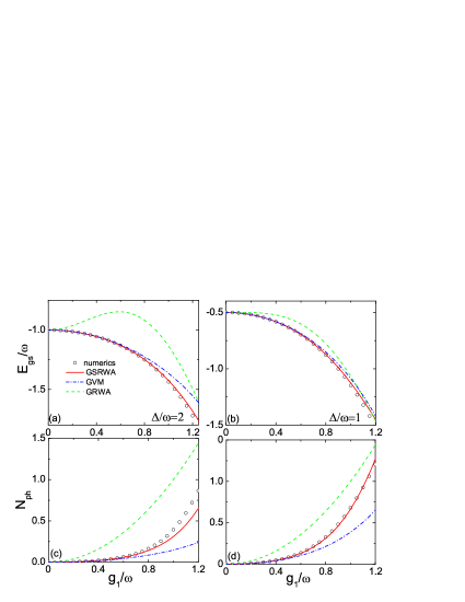
Figure 1: (Color online) (a) and (b) The ground-state energy $E_{gs}/\omega$ and (c) and (d) the corresponding mean photon number $N_{ph}$ (c-d) obtained analytically in the isotropic case as a function of $g_{1}/\omega$ for different detuning cases obtained by the GSRWA (solid lines), numerical simulation (circles), GVM (dashed-dotted lines), and GRWA (dashed lines) for the isotropic Rabi model.

Within the GSRWA, the optimal variables $\beta$ and $\lambda$ can be derived from minimizing the ground-state energy according to $\partial E_{gs}^{\mathtt{GSRWA}}/\partial\beta=0$ and $\partial E_{gs}^{\mathtt{GSRWA}}/\partial\lambda=0$ by

$$0=\beta\Delta e^{-4\lambda}e^{-2\beta^{2}\exp(-4\lambda)}+\omega\beta-\alpha,$$ (20)

$$0=-4\beta^{2}\Delta e^{-4\lambda}e^{-2\beta^{2}\exp(-4\lambda)}+\omega(e^{4\lambda}-e^{-4\lambda}).$$ (21)

When the dimensionless parameters $\lambda$ and $\beta$ are less than $1$, the displacement $\beta$ is given approximately by

$$\beta\simeq\frac{\alpha}{\omega+\Delta e^{-4\lambda}e^{-2\alpha^{2}/(\omega+\Delta)^{2}\exp(-4\lambda)}},$$ (22)

and the squeezing parameter is

$$\lambda\simeq\frac{\Delta}{2\omega}\frac{\alpha^{2}}{(\omega+\Delta)^{2}}.$$ (23)

Interestingly, $\lambda$ depends on the atom frequency $\Delta$, resulting in an important squeezing effect in lowering the ground-state energy as $\Delta$ increases. And $\beta$ is amended by adding the squeezing parameter as $\exp(-4\lambda)$ by comparing with $\beta$ in the GVM. With the increase in atom frequency $\Delta$ and the effective coupling strength $\alpha$, both the displacement and the squeezing play an important role in lowering the ground-state energy.

In particular, in the current experimental setups of the ultra-strong coupling, $g_{1}/\omega,g_{2}/\omega\simeq 0.1$, the optimal displacement $\beta$ is simplified as $\alpha/(\omega+\Delta)$, and one can obtain an explicit ground-state energy

$$E_{gs}^{\mathtt{GSRWA}} \simeq\omega\sinh^{2}[\frac{\Delta\alpha^{2}}{\omega(\omega+\Delta)^{2}}]-\frac{\alpha^{2}(\omega+2\Delta)}{(\omega+\Delta)^{2}}$$ (24)

$$-\frac{\Delta}{2}e^{-\frac{2\alpha^{2}}{(\omega+\Delta)^{2}}\exp[-\frac{2\Delta\alpha^{2}}{(\omega+\Delta)^{2}}]},$$

which exhibits an improvement over the one in the GVM $E_{gs}^{\mathtt{GVM}}=-\frac{\alpha^{2}(\omega+2\Delta)}{(\omega+\Delta)^{2}}-\frac{\Delta}{2}\mathtt{exp}[-\frac{2\alpha^{2}}{(\omega+\Delta)^{2}}]$ yu .

On the other hand, in the deep-strong coupling limit, $g_{1}/\omega\gg 1$, we derive approximately $\beta\simeq\alpha/\omega$ and $\lambda\simeq 0$ from the optimal Eqs. ( 20) and ( 21). Obviously, the squeezing effect disappears. The ground-state energy becomes

$$E_{gs}^{\mathtt{GSRWA}}\simeq-\frac{\alpha^{2}}{\omega}-\frac{\Delta}{2}e^{-\frac{2\alpha^{2}}{\omega^{2}}},$$ (25)

which is the same as that obtained by the GRWA with $\beta=\alpha/\omega$.

Figures  1 (a) and (b) show the ground-state energy in the GSRWA obtained analytically by the displacement $\beta$ ( 22) and the squeezing $\lambda$ ( 23) for large atom frequency. For weak coupling strength $g_{1}/\omega$, contribution from the coupling is small and the ground-state energies obtained by the four methods are equal. As $g_{1}$ increases, the oscillator state becomes the displaced state due to the coupling of the atom and the original oscillator. The variable displacement in the GSRWA or GVM becomes to play a role in lowering the ground-state energy, exhibiting lower energy than the GRWA results. As $g_{1}$ enters the ultra-strong coupling regime, $g_{1}/\omega\sim 0.5$, the squeezing effect becomes appreciable and the oscillator state should be a displaced-squeezed state instead of a displaced state. As a result, the GSRWA results agree well with the numerical ones ranging from weak to ultra-strong coupling regimes. However, the results from the GVM become worse for the ultra-strong coupling strength $g_{1}/\omega>0.8$, especially for the positive detuning $\Delta/\omega=2$ in Fig. 1 (a). The deviations of the GVM or GRWA become more noticeable as $\Delta/\omega$ increases. The reason for the failure is that the squeezing effect is underestimated in the GVM and GRWA with only the displacement transformation. Therefore, the squeezing effect becomes important as the coupling strength increases up to $g_{1}/\omega\sim 1$, especially for large atom frequency.

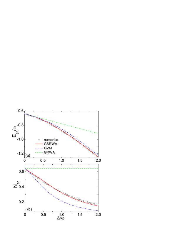
Figure 2: (Color online) (a)The ground-state energy $E_{gs}/\omega$ and (b) the mean photon number $N_{\mathtt{ph}}$ in the isotropic case as a function of $\Delta/\omega$ for the coupling strength $g_{1}/\omega=0.8$ by means of the GSRWA (solid lines), numerical simulation (circles), GVM (dash-dotted lines) and GRWA (dashed lines).

To show the squeezing effect dependent on the detunings $\Delta/\omega$, Fig. 2(a) shows the ground-state energy as a function of $\Delta/\omega$ for the ultra-strong coupling strength $g_{1}/\omega=0.8$. It shows an accuracy of the ground-state energy in the GSRWA for arbitrary detunings due to the squeezing effect in Eq.( 23) dependent on $\Delta/\omega$. However, there is a distinguished deviation of the GVM and GRWA results from negative detuning $\Delta/\omega<1$ to positive detuning $\Delta/\omega>1$. It reveals that the squeezing plays an important effect in lowering the ground-state energy as $\Delta/\omega$ increases.

We now discuss the mean photons number $N_{ph}=\langle a^{+}a\rangle$ in the ground state $|\tilde{G}\rangle$, which can be derived by

$$N_{ph}^{\mathtt{GSRWA}}=\omega\sinh^{2}2\lambda+\omega\beta^{2}.$$ (26)

The second term denotes the mean photon number in the GVM, and the first squeezing term shows an improvement of $N_{ph}$ by the GSRWA. One can obtain the mean photon number in the GVM  yu as

$$N_{ph}^{\mathtt{GVM}}=\omega\beta^{2}\simeq\frac{\omega\alpha^{2}}{[\omega+\Delta e^{-2\alpha^{2}/(\omega+\Delta)^{2}}]^{2}}.$$ (27)

For the GRWA with $\beta=\alpha/\omega$, the mean photon number simply is given by $N_{ph}^{\mathtt{GRWA}}=\omega\beta^{2}\simeq\alpha^{2}/\omega$, which is independent of $\Delta$. In terms of the analytical solution of the displacement $\beta$ ( 22) and squeezing $\lambda$ ( 23), the mean photon number under the GSRWA can explicitly be given by

$$N_{ph}^{\mathtt{GSRWA}} \simeq\omega\sinh^{2}[\frac{\Delta\alpha^{2}}{\omega(\omega+\Delta)^{2}}]$$ (28)

$$+\frac{\omega\alpha^{2}}{[\omega+\Delta e^{-4\lambda}e^{-2\alpha^{2}/(\omega+\Delta)^{2}\exp(-4\lambda)}]^{2}}.$$

It is observed that there is an oversimplified analytical treatment for the mean photon number in the GVM and GRWA, but the GSRWA with additional squeezing terms provides an efficient, yet accurate analytical expression.

The mean photon number is plotted as a function of the coupling strength $g_{1}/\omega$ for the positive detuning and resonance cases in Figs. 1 (c)(d). The GSRWA agrees well with the numerical ones from weak to ultra-strong coupling regimes. However, the GVM and GRWA results are qualitatively incorrect as the coupling strength increases.

Behavior of the mean photon number $N_{ph}$ dependent on $\Delta/\omega$ is plotted in Fig. 2 (b) for the ultra-strong coupling strength $g_{1}/\omega=0.8$. The results derived from the GSRWA are consistent with those of the numerical simulation from negative to positive detunings. For the large negative detuning $\Delta/\omega\ll 1$, the GVM results agree well with the numerical ones. However, as $\Delta/\omega$ increases, the GVM breaks down and the deviations becomes larger. And the GRWA keeps an incorrect constant in the whole detuning case, since the analytical $N_{ph}^{\mathtt{GRWA}}$ is independent of $\Delta$. It is concluded that the analytical results of the GSRWA with the squeezing is more accurate than those of the previous GVM or GRWA for arbitrary detuning even for the ultra-strong coupling strength $g_{1}/\omega\sim 1$.

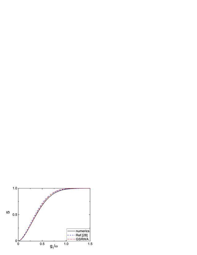
Figure 3: (Color online) The qubit-oscillator entanglement $S$ obtained by the GSRWA (dashed line) with the displacement in Eq. (22) and squeezing in Eq. (23) using the experiment parameters in Ref. yoshihara . The entanglement obtained by numerical simulation (solid line), and results in Ref. yoshihara (dashed-dotted line) are plotted for comparison.

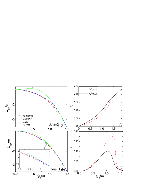
Figure 4: (Color online) (a) and (b) The ground-state energy $E_{gs}/\omega$ (a-b) in the anisotropic Rabi model with $\gamma>0$ as a function of $g_{1}/\omega$ for different detuning cases by means of the GSRWA (dashed lines), numerical simulation (circles), GVM (dashed-dotted lines) and GRWA (dotted lines) with the coupling strength $g_{2}=1.5g_{1}$. The corresponding (c) variable displacement $\beta$ and (d) squeezing $\lambda$ (d) as a function of $g_{1}/\omega$ obtained by the GSRWA for different detunings $\Delta/\omega=2$ (dashed line) and $\Delta/\omega=1$ (solid line).

Due to the recent advances in circuit QED setups, the ground state can be described by the Schrödinger-cat-like entangled state between the qubit and the oscillator beyond the ultra-strong coupling, where the oscillator state was described as the displaced state $\mathtt{exp}[\pm g_{1}/\omega(a^{\dagger}-a)]$ yoshihara . In our method, the ground state $|\tilde{G}\rangle$  (III) is improved by the displaced-squeezed oscillator state, which is expected to be a well-defined Schrödinger-cat-like entangled state. The progress is made by using the entangled state $|\tilde{G}\rangle$ to estimate the qubit-oscillator entanglement $S$. Considering the expression $V^{+}e^{\beta\left(a^{+}-a\right)}V=e^{\beta^{\prime}(a^{+}-a)}$ with $\beta^{\prime}=\beta\eta_{2}$, the overlap of two displaced-squeezed oscillator states is obtained as ${}_{s}\langle 0|e^{\beta\left(a-a^{+}\right)}e^{-\beta\left(a^{+}-a\right)}|0\rangle_{s}=e^{-2\beta^{\prime 2}}$. It leads to the qubit’s reduced density matrix $\rho_{a}$ by tracing out the oscillator degrees of freedom,

$$\rho_{a}=\frac{1}{2}\left(\begin{array}[]{cc}1&e^{-2\beta^{\prime 2}}\\ e^{-2\beta^{\prime 2}}&1\end{array}\right),$$

where the eigenvalues of $\rho_{a}$ are $p_{\pm}$ $=(1\pm e^{-2\beta^{\prime 2}})/2$. The entanglement can be measured by the von Neumann entropy Popescu ; Wang of the qubit:

$$S=-p_{+}\log_{2}p_{+}-p_{-}\log_{2}p_{-}.$$ (29)

The entanglement is modified by $\beta^{\prime}$ instead of the displacement $\beta=g_{1}/\omega$ in previous results yoshihara . Fig.3 shows the qubit-oscillator entanglement $S$ using the analytical displacement in Eq. (22) and the squeezing in Eq. (23), with fitted parameters of the experimental results $\omega/2\pi=5.711~{}\mathrm{GHz}$ and $\Delta=0.441~{}\mathrm{GHz}$. Besides the validity of the GSRWA as well as of Ref. yoshihara in the deep-strong coupling regime, $g_{1}/\omega>1$, a noticeable improvement by the GSRWA is observed in the ultra-strong coupling regimes. This demonstrates the great potential of our GSRWA approach to be applied in future experiments for the ultra-strong coupling strength by the displaced-squeezed oscillator state instead of the original displaced state.

Dominated coupling of the CRW interaction ($\gamma>0$): For the anisotropic Rabi model, the different couplings allow us to vary the CRW interaction independently and explore the effects of it on some quantum properties. We first study the ground-state energy in the case of the dominated coupling of the CRW term, $g_{2}\geq g_{1}$ with $\gamma>0$.

Averaging over the ground state $|G\rangle$ ( 17) the ground-state energy is obtained as

$$E_{gs}^{\mathtt{GSRWA}} =\omega\sinh^{2}2\lambda+\omega\beta^{2}-2\beta\alpha$$ (30)

$$-(\frac{\Delta}{2}+2\gamma\beta e^{-4\lambda})e^{-2\beta^{2}\exp(-4\lambda)}.$$

The optimal values of $\beta$ and $\gamma$ are obtained numerically by minimizing the ground-state energy according to $\partial E_{gs}^{\mathtt{GSRWA}}/\partial\beta=0$ and $\partial E_{gs}^{\mathtt{GSRWA}}/\partial\lambda=0$. By setting the squeezing $\lambda=0$ in Eq.( 30), the displacement $\beta$ in the GVM is optimized by minimizing the ground-state energy

$$E_{gs}^{\mathtt{GVM}}=\omega\beta^{2}-2\beta\alpha-(\frac{\Delta}{2}+2\gamma\beta)e^{-2\beta^{2}}.$$ (31)

Meanwhile, the ground-state energy in the GRWA with $\beta=\alpha/\omega$ is obtained easily as $E_{gs}^{\mathtt{GRWA}}=-\alpha^{2}/\omega-(\frac{\Delta}{2}+2\gamma\alpha/\omega)e^{-2\alpha^{2}/\omega^{2}}$.

Figure 4 displays the ground-state energy $E_{gs}/\omega$ as a function of the coupling strength $g_{1}$ for $g_{2}=1.5g_{1}$ under different detunings $\Delta/\omega=2$ (a) and $\Delta/\omega=1$ (b) by means of four methods. For the coupling strength $g_{1}/\omega<0.5$, both results of the GSRWA and the GVM agree well with the numerical ones. As $g_{1}/\omega$ increases to $0.8$, the GVM deviates from the numerical results. This deviation becomes more obvious for positive detuning $\Delta/\omega=2$. However, the GSRWA results coincide with those of the numerical simulation well in the ultra-strong coupling regime except for a small discrepancy in the deep-strong coupling regime for $\Delta/\omega=2$. The GRWA produces unreasonable results in the ultra-strong coupling regime. It is demonstrated that the GSRWA results are much better than the GVM and GRWA ones in the anisotropic case.

The advantage of the GSRWA lies in the contribution from the variable squeezing and displacement. The optimum values for $\beta$ and $\lambda$ have interesting dependences on the coupling $g_{1}/\omega$ and the detunings $\Delta/\omega$, as shown in Figs. 4(c) and  4(d). As $g_{1}/\omega$ increases, effects of both displacement and squeezing transformations become to play an important role in lowering the ground-state energy. $\beta$ and $\lambda$ develop, and in particular, the squeezing $\lambda$ increases as the coupling strengthens to a maximum value, and then decreases in the deep-strong coupling regime, which is qualitatively similar to the prediction by the analytical $\lambda$ in the isotropic case. And the larger $\Delta/\omega$ is chosen, the larger the value of the maximum $\lambda_{max}$ reaches. Thus the squeezing effects can not be underestimated with the increase in $\Delta/\omega$. In the deep-strong coupling limit, $\beta$ nearly increases linearly with $g_{1}/\omega$, and $\lambda$ decays to zero, which is the result predicted by the GRWA. Therefore, the contributions of both the displacement and squeezing transformations are significant especially for the ultra-strong coupling strength $g_{1}/\omega\sim 1$, where the GVM and the GRWA are no longer valid.

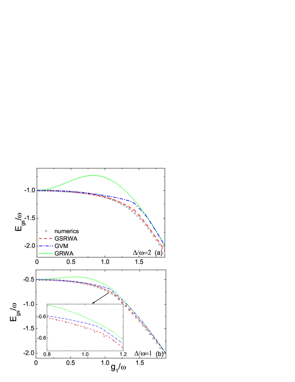
Figure 5: (Color online) Ground-state energy $E_{gs}/\omega$ in the anisotropic Rabi model with $\gamma<0$ as a function of $g_{1}/\omega$ by means of the GSRWA (dashed lines), numerical simulation (circles), GVM (dashed dotted lines) and GRWA (dotted lines) for $g_{2}=0.5g_{1}$ for different detunings (a)$\Delta/\omega=2$ and (b) $\Delta/\omega=1$.

Dominated coupling of the RW interaction ($\gamma<0$): For the anisotropic case of the dominated coupling of the RW interaction with $\gamma<0$, $g_{2}<g_{1}$, energy-level crossing between the ground state and the first-excited state occurs due to the competition between the rotating and counter-rotating interactions xie . And the first excited state consisting of $|0\rangle|+z\rangle$ and $|1\rangle|-z\rangle$ is expected to be the ground state when the coupling strength exceeds the crossing point xie .

In terms of the basis $|0\rangle|+z\rangle$ and $|1\rangle|-z\rangle$, the transformed Hamiltonian ( II) obtained by the GSRWA is written in the matrix form as

$$H_{\mathtt{GSRWA}}=\left(\begin{array}[]{cc}\eta_{0}+f(0)&\eta_{2}(\alpha-\beta)+P_{1,0}\\ \eta_{2}(\alpha-\beta)+P_{1,0}&\eta_{0}+\eta_{1}-f(1)\end{array}\right),$$ (32)

where $P_{1,0}=\frac{\Delta}{2}R_{1,0}-\gamma\eta T_{1,0}$. The eigenvalue of the first exited state is given by

$$E_{gs}^{\mathtt{GSRWA}} = \eta_{0}+\frac{\eta_{1}+f(0)-f(1)}{2}$$ (33)

$$-\frac{1}{2}\sqrt{[f(0)-\eta_{1}+f(1)]^{2}+4P_{1,0}^{2}},$$

and the corresponding first-excited state takes the form as

$$|\varphi_{1}\rangle=\cos\theta|0,+z\rangle+\sin\theta|1,-z\rangle,$$ (34)

with $\tan\theta=\frac{2P_{1,0}}{f(1)+f(0)-\eta_{1}-\sqrt{[f(0)-\eta_{1}+f(1)]^{2}+4P_{1,0}^{2}}}$.

For the crossing of the ground state and the first-excited state, the crossing point $g_{c}$ is determined numerically when the ground-state energy ( 30) is equivalent to the first-excited energy, $E_{1}^{\mathtt{GSRWA}}=E_{gs}^{\mathtt{GSRWA}}$. After the crossing point, $\beta$ and $\lambda$ are determined variationally according to the equations of minimizing the first-excited energy by $\partial E_{1}^{\mathtt{GSRWA}}/\partial\beta=0$ and $\partial E_{1}^{\mathtt{GSRWA}}/\partial\lambda=0$. Similarly, one can obtain the corresponding ground-state energy after the crossing point by setting $\lambda=0$ for the GVM and $\beta=\alpha/\omega$, $\lambda=0$ for the GRWA in Eq. ( 33).

Figure 5 shows the ground-state energy $E_{gs}$ as a function of the coupling strength $g_{1}/\omega$ by different methods under different detunings. $E_{gs}$ obtained by the GSRWA is consistent with the numerical ones even for the ultra-strong coupling strength up to $g_{1}/\omega\sim 1$. However, we can see that the GVM with only the variable displacement deviates from the numerical results in the ultra-strong coupling regime $g_{1}/\omega>0.8$, and the one by the fixed $\beta$ under the GRWA shows a dramatic deviation even in the weak coupling regime. Moreover, the GVM and the GRWA get worse as the detuning $\Delta/\omega$ increases to $2$ in Fig. 5(a). It exhibits an overall improvement of the GSRWA by adding a dimensionless variable squeezing to the original GVM or GRWA in the anisotropic Rabi model.

IV Conclusion

We present the generalized squeezing rotating-wave approximation, which depends on the optimal displacement and squeezing parameters, as determined variationally. The approach by adding the squeezing transformation improves the previous generalized variational method and generalized RWA only with the displacement transformation. The ground state is obtained as a well-defined Schrödinger-cat-like entangled state with the displaced-squeezed oscillator state instead of the displaced state. For the isotropic Rabi case, the analytical expression of the ground-state energy and the mean photon number agree well with the numerical ones especially for the ultra-strong coupling strength up to $g_{1}/\omega\sim 1$, whereas the previous results with only the displacement show distinguished deviation for large atom frequency. For the anisotropic case, the ground-state energy obtained by the presented approach is more accurate than previous results. It demonstrates that the contribution of the squeezing is significant in the ground state in the ultra-strong coupling regime especially for large atom frequency. In additional, an efficient treatment for excited states is expected to be proposed in future work by considering the squeezing effect. The analytical solution presented here can easily be implemented to simulate superconducting qubit-oscillator systems for ultrastrong-coupling strengths up to $g/\omega\sim 1$, which is accessible in recent circuit QED experiment setups yoshihara .

V Acknowledgments

This work was supported by the Chongqing Research Program of Basic Research and Frontier Technology (Grant No.cstc2015jcyjA00043), and the Research Fund for the Central Universities (Grants No.106112016CDJXY300005, and No. CQDXWL-2014-Z006).

Email:yuyuzh@cqu.edu.cn

References

- (1) I. I. Rabi, Phys. Rev. 51,652 (1937).
- (2) K. Baumann, C. Guerlin, F. Brennecke, and T. Esslinger, Nature (London)464, 1301(2010).
- (3) D. Nagy, G. Kónya, G. Szirmai, and P. Domokos, Phys. Rev. Lett. 104, 130401(2010).
- (4) F. Dimer, B. Estienne, A. S. Parkins, and H. J. Carmichael,Phys. Rev. A 75, 013804(2007).
- (5) A. Wallraff et al., Nature (London)431, 162(2004).
- (6) T. Niemczyk et al., Nature Physics 6, 772(2010).
- (7) P. Forn-Díaz et al., Phys. Rev. Lett. 105, 237001 (2010).
- (8) A. Fedorov et al., Phys. Rev. Lett. 105, 060503 (2010).
- (9) E.T. Jaynes, and F.W. Cummings, Proc. IEEE. 51, 89(1963).
- (10) S. I. Erlingsson, J. C. Egues, and D. Loss, Phys. Rev. B 82, 155456(2010).
- (11) Y. Yi-Xiang, J. W. Ye, and W. M. Liu, Sci. Rep. 3, 3476(2013).
- (12) Q. T. Xie, S. Cui, J. P. Cao, L. Amico, and H. Fan, Phys. Rev. X 4, 021046(2014).
- (13) B. R. Judd, J. Phys. C 12, 1685(1979).
- (14) A. L. Grimsmo, and S. Parkins, Phys. Rev. A 87, 033814(2013).
- (15) D. Braak, Phys. Rev. Lett. 107, 100401(2011).
- (16) M. Tomka, O. El. Araby, M. Pletyukhov, and V. Gritsev, Phys. Rev. A 90, 063839 (2014).
- (17) Q. H. Chen, C. Wang, S. He, T. Liu, and K. L. Wang, Phys. Rev. A 86, 023822 (2012).
- (18) E.K. Irish, Phys. Rev. Lett. 99, 173601(2007).
- (19) Y. Y. Zhang, Q. H. Chen, and Y. Zhao, Phys. Rev. A 87, 033827(2013); Y. Y. Zhang, Q. H. Chen, ibid 91, 013814(2015).
- (20) S. Agarwal, S. M. Hashemi Rafsanjani, and J. H. Eberly, Phys. Rev. A 85, 043815 (2012).
- (21) S. Ashhab, Phys. Rev. A 87, 013826 (2013).
- (22) Y. Zhang, G. Chen, L. Yu, Q. Liang, J. Q. Lang, and S. T. Jia, Phys. Rev. A 83, 065802 (2011).
- (23) V. V. Albert, G. D. Scholes, and P. Brumer, Phys. Rev. A 84, 042110 (2011).
- (24) C. J. Gan, and H. Zheng, Eur. Phys. J. D 59,473 (2010).
- (25) G. F. Zhang, and H. J. Zhu, Sci. Rep 5, 8756 (2015).
- (26) Z. J. Ying, M. X. Liu, H. G. Luo, H. Q. Lin, and J. Q. You,Phys. Rev. A 92, 053823 (2015).
- (27) M. J. Hwang, R. Puebla, and M. B. Plenio, Phys. Rev. Lett. 115, 180404 (2015).
- (28) F. Yoshihara, T. Fuse, S. Ashhab, K. Kakuyanagi, S. Saito, and K. Semba, arXiv: 1602. 00415.
- (29) S. Popescu, and D. Rohrlich, Phys. Rev. A. 56, R3319 (1997).
- (30) X. Wang, and B. Sanders, J. Phys. A. 38, L67 (2005).