Topological insulating phases from two-dimensional nodal loop semimetals

Abstract

Starting from a minimal model for a 2D nodal loop semimetal, we study the effect of chiral mass gap terms. The resulting Dirac loop anomalous Hall insulator’s Chern number is the phase winding number of the mass gap terms on the loop. We provide simple lattice models, analyze the topological phases and generalize a previous index characterizing topological transitions. The responses of the Dirac loop anomalous Hall and quantum spin Hall insulators to a magnetic field’s vector potential are also studied both in weak and strong field regimes, as well as the edge states in a ribbon geometry.

I Introduction

The nontrivial topological properties of fermions, which have attracted great attention recently, stem from their low energy Dirac-like band dispersion and its associated chiralities. Differently from conventional physical phases, topological phases are classified by discrete topological invariants of occupied bands, rather than continuous order parametersreview1 ; review2 . Depending on its time reversal, particle-hole and chiral symmetries, a gapped system, insulator or superconductor, can be classified into ten topological classes, five of which can support topologically nontrivial phases depending on the dimension of the systemclasses . In an insulating system, the bulk gap contains nontrivial boundary states whose chirality or helicity is determined by the topological invariants. In superconductors, the possibility of realizing Majorana fermions has spurred intense research because of their potential application in quantum computationalicea .

In some three dimensional systems, there may also be linear band touching at discrete Dirac or Weyl points, or “nodes”, in the Brillouin Zone (BZ). Dirac and Weyl semimetals have been the focus of intense researchWan ; Delplace ; Hou ; Young ; Ganeshan , as they are gapless systems which can exhibit topological properties. A Dirac semimetal enjoys both time-reversal and inversion symmetries. When one of these symmetries is broken, Weyl nodes with opposite chiralities separated in momentum space may appear and the semimetal exhibits surface Fermi arcs and the chiral anomalyNN1 . Examples of Dirac semimetals are Na₃Bi, Cd₃As₂zawng ; sxu ; zklu ; zwang2 ; zkliu ; neupane ; borisenko . The Weyl semimetal state has been experimentally confirmed in the TaAs familyhweng ; shuang ; sxu2 ; lv ; lyang .

More recently, a new class of three-dimensional semimetal with nodal lines has attracted growing interestMullen ; 3D_loop ; Yan , following the suggestion for its realization in the hyperhoneycomb latticeMullen . In this case, the linear band touching occurs along a closed loop in the BZ. The concept of nodal loop semimetal is relatively new and awaits further investigation.

In addition to the above types of three-dimensional topological semimetals (Dirac, Weyl and nodal line), a more recent proposal for the concept of a two-dimensional nodal line semimetal has emerged and a suggestion for its physical realization in a new composite lattice composed of interpenetrating kagome and honeycomb lattices has been presentedLu . Spin-orbit coupling can open a small gap at the node line, resulting in a novel topological crystalline insulator.

Motivated by these recent developments, we here study the nodal loop (NL) semimetal in two dimensions, for spinless fermions. The introduction of mass gap terms may lead to topological insulating phases. We derive an expression for the Chern number of the resulting Dirac loop anomalous Hall insulator (DLAHI). The Chern number is equivalent to the winding number of the mass terms’ phase along the loop and can be regarded as the loop’s chirality. We examine the topological transitions that take place as model parameters change and generalize a previous index that characterizes such transitions. The effect of a magnetic field on a DLAHI is also studied and compared to the case of Dirac point systems.

In Section II we introduce the minimal model for a NL semimetal, consider a mass gap, and study the topological properties of the DLAHI. Section III is devoted to the study of magnetic field effects. In Section IV we summarize our results and make some concluding remarks.

II Topological insulator in Generalized 2D nodal loop semimetal

II.1 Minimal Model and Topological Invariant

To model a nodal loop semimetal in two dimensions, it is necessary for the system to have at least two bands, and the Hamiltonian can be written as

$$H=\bm{h}(\bm{k})\cdot\bm{\tau},$$ (1)

where $\tau_{\alpha}$ ($\alpha=1,2,3$) are the Pauli matrices acting on sublattice (“pseudo-spin”) space and the Bloch wave vector $\bm{k}=(k_{x},k_{y})$ runs over the Brillouin zone (BZ). We first consider a minimal Hamiltonian with a nodal circular loop3D_loop :

$$h_{3}=\hbar v_{0}(k-k_{0}),$$ (2)

Here $k=\sqrt{k_{x}^{2}+k_{y}^{2}}$ and $k_{0}$ is the loop radius. Equation (2) is supposed to be a valid approximation in the region $k\approx k_{0}$ of the BZ. This Hamiltonian gives a NL semimetal where the valence and conduction bands cross at $k=k_{0}$ if $h_{1}=h_{2}=0$. In a doped system, the Fermi surface would be a ring with radius $k_{0}$, but we shall not consider doped systems below. $h_{1}$ and $h_{2}$ can be viewed as two independent mass terms. Nonzero $h_{1}$ and $h_{2}$ may open a gap and turn the system into an insulator if only the lower (valence) band is occupied. We take the band gap $\Delta\equiv\sqrt{h_{1}^{2}+h_{2}^{2}}\ll\hbar v_{0}k_{0}$. It may take on a constant value on the loop, or have some $\bm{k}$ dependence. A plot of the dispersion is shown in Fig. 1.

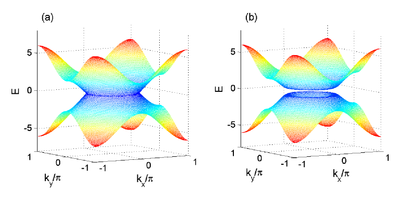
Figure 1: (color online). The dispersion relation of a NL semimetal (a). Panel (b) shows the gapped spectrum.

The topological properties of this model can be characterized by the Chern number, $C$, of the occupied band, which is defined as

$$C = \frac{1}{2\pi}\int V_{\bm{k}}dk_{x}dk_{y}\,,$$ (3)

$$V_{\bm{k}} = \partial_{k_{x}}A_{k_{y}}-\partial_{k_{y}}A_{k_{x}}\,,$$ (4)

where $V_{\bm{k}}$ is the Berry curvature and $A_{\alpha}=i\langle\varphi(\bm{k})|\partial_{\alpha}|\varphi(\bm{k})\rangle$ is the Berry connectionBerry , $\varphi(\bm{k})$ is a Bloch eigenstate of the occupied band, and the integral is over the two-dimensional Brillouin zone. Equation (4) yields a well defined result provided that the loop is gapped.

We shall now show that a simple expression for $C$ can be obtained which involves only the circulation of the phase of $h_{1}-ih_{2}$ along the loop. For the two-band system described by Eq.(1), the Berry curvature of the lower band takes on the familiar form,

$$V_{\bm{k}} = \frac{1}{2|\bm{h}|^{3}}\frac{\partial\bm{h}}{\partial k_{x}}\times\frac{\partial\bm{h}}{\partial k_{y}}\cdot\bm{h}\,,$$ (5)

where $|\bm{h}|=\sqrt{h_{1}^{2}+h_{2}^{2}+h_{3}^{2}}$. Using polar coordinates in momentum space, $(k,\theta)$, we write $(k_{x},k_{y})=k(\cos{\theta},\sin{\theta})$. We rewrite the Berry curvature in polar coordinates and, considering that the contribution to the integral (3) comes from the vicinity of the loop where Eq.(2) holds, we obtain

$$C = \frac{\hbar v_{0}}{4\pi}\int\frac{dkd\theta}{|\bm{h}|^{3}}\left(h_{2}\partial_{\theta}h_{1}-h_{1}\partial_{\theta}h_{2}\right)$$ (6)

The integration over $k$ can be performed under the assumption that the gap $\Delta\ll\hbar v_{0}k_{0}$. This allows us to extend the integration limits of $k$ to the whole real axis and obtain:

$$C = {\rm sgn}(v_{0})\int_{0}^{2\pi}\frac{d\theta}{2\pi}\frac{h_{2}\partial_{\theta}h_{1}-h_{1}\partial_{\theta}h_{2}}{h_{1}^{2}+h_{2}^{2}}\,,$$ (7)

where the integration is performed on the loop $h_{3}=0$. The expression (7) is just the winding number for the phase of $h_{1}-ih_{2}$. The above derivation may be regarded as an extension of the contribution from a single Dirac point to the Chern numbereu , which can be $\pm 1/2$. By analogy, equation (7) assigns a chirality to the gapped loop. While a fermionic system must have an even number of Dirac pointsNN , there may be only one, or arbitrary number of NL’s.

The above Chern number is ill defined when the gap closes, $h_{1}=h_{2}=0$, as the integrand of Eq.(7) diverges. At a topological phase transition the gap closes and a definition of a $\mathbb{Z}$ index characterizing the transition can be achieved in the extended three dimensional parameter space, $(\bm{k},\eta)$, where $\eta$ is a transition driving parameterLinhu . We assume the system to be an insulator for general $\eta$ and the gap closes at $\eta=\eta_{0}$. If the gap closes at one or more discrete points in the BZ, a topological number $C_{p}$ can be calculated as the flux of the Berry curvature through a sphere $\bm{S}$ enclosing each of these points in the parameter space of $(\bm{k},\eta)$,

$$C_{p}=\frac{1}{2\pi}\oiint\bm{V}\cdot d\bm{S}\,,$$ (8)

where $\bm{V}=\nabla\times i\langle\varphi(\bm{k},\eta)|\nabla|\varphi(\bm{k},\eta)\rangle$ is the Berry curvature in the extended parameter space. The summation of $C_{p}$ over every gap closing point gives the change of the Chern number $C$ across the transitionLinhu .

We can extend the above index to the case of a nodal loop semimetal, by defining a similar index, $C_{l}$, as the Berry curvature flux through a torus enclosing the loop. In the parameter space of $\bm{k}$ and $\eta$, this torus can be written as

$$k_{x} = [k_{0}+r\cos{\phi}]\cos{\theta}\,,$$

$$k_{y} = [k_{0}+r\cos{\phi}]\sin{\theta}\,,$$

$$\eta = \eta_{0}+r\sin{\phi}\,,$$ (9)

where $\phi$ is a new angular parameter on the torus and $r$ is the tube radius as shown in Fig.2. We may recast the surface integral in Eq.(8) using equations (9) and $\theta$, $\phi$ as integration variables, as

$$C_{l} = \frac{1}{2\pi}\int\int V_{\phi,\theta}d\phi d\theta\,,$$

$$V_{\phi,\theta} = \partial_{\phi}A_{\theta}-\partial_{\theta}A_{\phi}\,.$$ (10)

The value of $C_{l}$ is independent of $r$ as long as no gap closing point exists other than the nodal loop within the torus. This index, $C_{l}$, can serve as a topological invariant which gives the change of Chern number, $C$, at a transition where $\eta=\eta_{0}$.

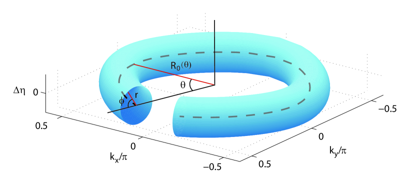
Figure 2: (color online). The torus in Eq.(9) in the parameter space $(\mathbf{k},\Delta\eta\equiv\eta-\eta_{0}$. The dashed line is the nodal loop when $\eta_{0}=0$. The flux of $\bm{V}$ though the torus surface gives the index $C_{l}$.

II.2 Specific models

We now provide some specific lattice models to illustrate the topological phases of a 2D nodal loop. Note that in a lattice model, the nodal loop is not a perfect circle in the BZ, so the loop radius $k_{0}$ is actually a function of the polar coordinate $\theta$, $k_{0}=k_{0}(\theta)$. Chern numbers for these lattice models are calculated numerically with the method described in Ref.ChernNum . Following this technique, the parameter space $(k_{x},k_{y})$, or $(\theta,\phi)$ for the calculation of $C_{l}$, is discretized and the circulations of the Berry connection on small plaquettes is performed.

We first consider the following model for the vector $\bm{h}(\bm{k})$ in Eq.(1):

$$h_{1}(\bm{k}) = \lambda\sin{k_{y}}+M$$

$$h_{2}(\bm{k}) = -\lambda\sin{k_{x}}$$

$$h_{3}(\bm{k}) = \mu-2(\cos{k_{x}}+\cos{k_{y}}).$$ (11)

The condition $h_{3}=0$ gives a nodal loop around the origin for $0<\mu<4$, or around the point $(\pi,\pi)$ for $-4<\mu<0$. We shall take $\mu=2$ below. When $M=0$, this model is also known as the Qi-Wu-Zhang model for spin-1/2 systemsQWZ . The term $M$ couples two pseudospin components at the same lattice site.

Model (11), for $4>\mu>0$, has two different topologically phases with $C=0$ or $C=-1$. In Fig. 3(a) we show the phase diagram with $\mu=2$. The topological phase boundary is given by $|\lambda|=M$, where the gap closes at a single point $\bm{k}=(0,-\mathrm{sgn}(\lambda\cdot M)\pi/2)$, except in the case $\lambda=M=0$, where the system is a nodal loop semimetal. In Figs. 3(b)-(g) we plot $(h_{1}(\theta),-h_{2}(\theta))$ for $h_{3}=0$, with $\theta$ varying from $0$ to $2\pi$, for different parameter choices. The Chern number $C=-1$ when $h_{1}-ih_{2}$ winds clockwise around the origin, in accordance with equation (7).

We now study the topological transitions that take place as the parameters $\lambda$ and $M$ change, either independently or along a chosen curve in the $(\lambda,M)$ plane. We start by examining two cases where the spectral gap closes over the whole loop, at the transition. A case where $M=0$ and $\lambda$ varies is plotted as a red dashed line in Fig. 3(a). Going along such a trajectory, no topological phase transition exists, as $C=-1$ always. Now consider the case where $M=\lambda\left(1-\lambda\right)$, which is plotted as the red curve in Fig. 3(a): a transition between $C=0$ and $C=-1$ phases occurs at $M=\lambda=0$. We use equation (10) to calculate the index $C_{l}$, where we identify the driving parameter $\eta$ with $\lambda$ and take the torus inner radius $r=10^{-4}$ in Eq.(9). Equation (10) then gives $C_{l}=0$ and $C_{l}=-1$ for these two cases, respectively, which indicates the change of $C$ at the transition point.

In Figs. 3(b)-(d) we show how the winding path $(h_{1}(\theta),-h_{2}(\theta))$ evolves for a topological phase transition where the gap closes at only one point on the loop, and the system evolves from $C=0$ to $C=-1$. For this case, equation (8) gives $C_{p}=-\mathrm{sgn}(\lambda\cdot M)$, as expected. Similarly, Figs. 3(e)-(g) show the winding paths of $h_{1}-ih_{2}$ as the model evolves with $-0.2\leq\lambda\leq 0.2$ and $M=\lambda\left(1-\lambda\right)$. For this case we obtain $C_{l}=-1$. Note that Figs. 3(c) and (f) show winding paths for two gapless spectra: panel (c) shows the situation where the gap closes at only one point of the loop; panel (f) depicts the case where the gap vanishes over the whole loop.

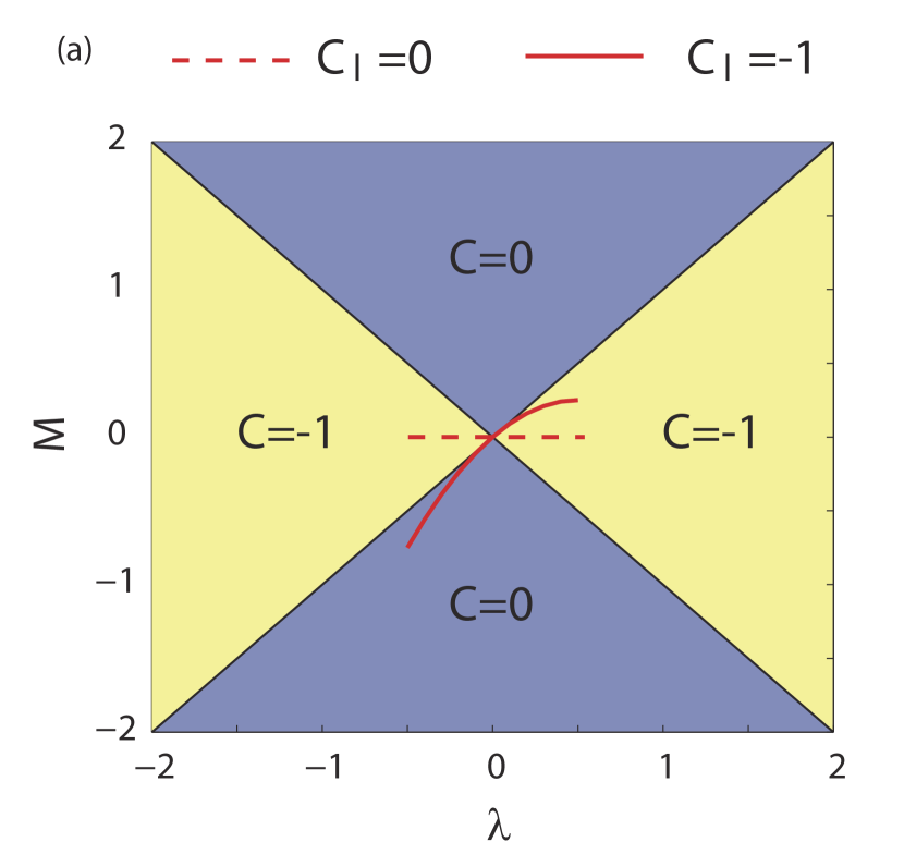
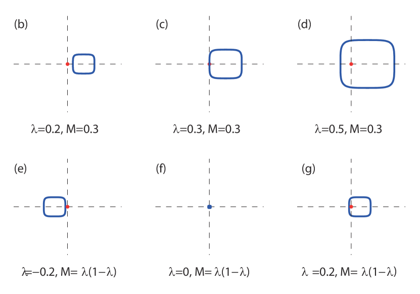
Figure 3: (color online). Panel (a) shows the phase diagram of model (11). The red and dashed lines are trajectories along which $C_{l}$ is calculated, as explained in the text. Panels (b)-(g) show winding paths, $(h_{1}(\theta),-h_{2}(\theta))$, as $0\leq\theta<2\pi$ and $h_{3}=0$. The direction of the winding path is clockwise for each case, yielding $C=-1$ when it encloses the origin, according to equation (7).

In the above lattice model, the Chern number may only be $\pm 1$ or $0$, as the winding path may go around the origin no more than once. However, if the mass terms $h_{1}$ and $h_{2}$ contain higher harmonics, the winding path will be more complicated and the system may have higher Chern number phases. As an example, we can choose the vector $\bm{h}(\bm{k})$ as

$$h_{1}(\bm{k}) = \lambda\sin(2k_{y})+M\,,$$

$$h_{2}(\bm{k}) = -\lambda\sin(2k_{x})\,,$$

$$h_{3}(\bm{k}) = \mu-2(\cos k_{x}+\cos k_{y})\,.$$ (12)

In Fig.4 we plot $(h_{1}(\theta),-h_{2}(\theta))$ for different parameter choices together with the corresponding Chern numbers. Panels (a)-(c) illustrate how $\mu$ changes the shape of the winding paths. and panels (d)-(f) show how $M$ changes the position of the winding path relative to the origin. $\lambda$ will change the size of the path (not shown in the figures).

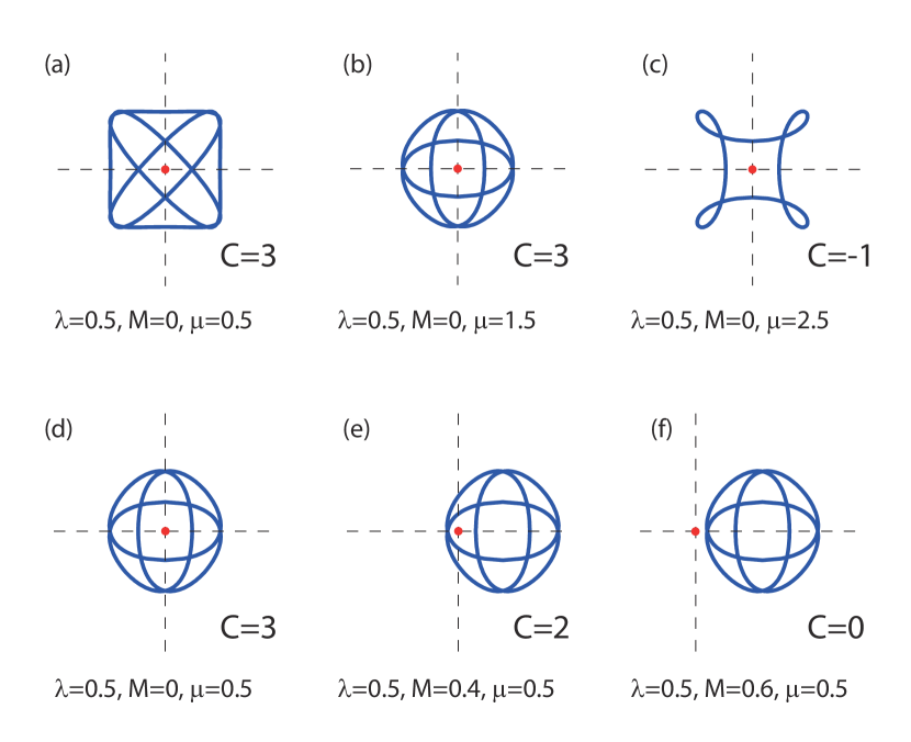
Figure 4: (color online). Winding paths $(h_{1}(\theta),-h_{2}(\theta))$ for model (12) for different parameter choices. The direction of the winding path is anti-clockwise except in (c), where it is clockwise.

In the recent proposalLu for the realization of the 2D nodal loop system in a kagome-honeycomb mixed lattice, spin-orbit terms were shown to introduce mass gap terms with $d_{xy}$ and $d_{x^{2}-y^{2}}$ symmetry. The system considered is time-reversal invariant and such terms yield $C=\pm 2$ in two effectively decoupled subspaces.

III Magnetic field

We now take the nodal loop Hamiltonian (1)-(13) as a model for spinless fermions on a lattice and analyze the effect of a magnetic field’s vector potential.

In the case of the anomalous Hall insulator with Dirac points, it has been shown that a weak field turns the system into a metal with half-filled Landau levels (LLs)haldane1988 ; Morais ; canadianos ; eu , while a topologically trivial insulator remains insulating under the field.

In order to understand the effect of a weak magnetic field on a NL, we follow the same procedure as in Refeu and introduce a vector potential, $\bm{A}$, which minimally couples to the orbital degrees of freedom, $-i\hbar\nabla\rightarrow-i\hbar\nabla-e\bm{A}$, where $e<0$ denotes the electron charge. It is convenient to replace Eq.(2) with

$$h_{3}=\hbar^{2}\frac{k^{2}-k_{0}^{2}}{2m}\,,$$ (13)

which, when linearized yields Eq.(2). We rewrite (13) in real space as:

$$h_{3}=-\hbar^{2}\frac{\partial_{x}^{2}+\partial_{y}^{2}+k_{0}^{2}}{2m}$$ (14)

If we further choose constant $h_{1(2)}$ with $\sqrt{h_{1}^{2}+h_{2}^{2}}\equiv\Delta\ll\frac{\hbar^{2}k_{0}^{2}}{2m}$, then the NL becomes gapped is a topologically trivial insulator at half-filling. We write $\bm{A}=B(0,x,0)$ and the wave functions as:

$$\psi_{\kappa,n} = e^{i\kappa y}\phi_{n}\left(x-\frac{\hbar\kappa}{eB}\right)\cdot\left(\begin{array}[]{c}\alpha\\ \beta\end{array}\right)\,.$$ (17)

Here, $n=0,1,...$ denotes the LL index, $\omega_{c}=|eB|/m$ denotes the cyclotron frequency, and $\phi_{n}(x)$ is a harmonic oscillator wave function. The column vector $(\alpha,\beta)^{T}$ solves the eigenproblem:

$$\left\{\left[\left(n+\frac{1}{2}\right)\hbar\omega_{c}-\frac{(\hbar k_{0})^{2}}{2m}\right]\tau_{3}+h_{1}\tau_{1}+h_{2}\tau_{2}\right\}\left(\begin{array}[]{c}\alpha\\ \beta\end{array}\right)=E_{n}\left(\begin{array}[]{c}\alpha\\ \beta\end{array}\right)\,,$$ (22)

and the energy levels are given by:

$$E_{n} = \pm\sqrt{\left[\left(n+\frac{1}{2}\right)\hbar\omega_{c}-\frac{(\hbar k_{0})^{2}}{2m}\right]^{2}+\Delta^{2}}\,.$$ (23)

The lowest LL ($n=0$) is far from the Fermi level if $\hbar\omega_{c}\ll(\hbar k_{0})^{2}/(2m)$. At half-filling the lower ”-” branch LL’s are fully occupied and the ones close to the Fermi level have high index $n=N$ such that $\left(N+1/2\right)\hbar\omega_{c}\approx(\hbar k_{0})^{2}/(2m)$.

The charge Hall conductance, $\sigma_{yx}$, takes on quantized values between the LLs. Each filled LL contributes $e^{2}/h$ to $\sigma_{yx}$. In the loop gap, $\sigma_{yx}=0$.

Because high order LLs are close to Fermi level, one may consider the semiclassical dynamics in the magnetic field. The semiclassical motion is determined by the equations:

$$\hbar\dot{\bm{k}}=ev_{\bm{k}}\times\bm{B}\,,\qquad\dot{\bm{r}}=v_{\bm{k}}$$ (24)

where the group velocity, $v_{\bm{k}}$, in the upper/lower band obeys $\hbar v_{\bm{k}}=\pm\partial|\bm{h}|/\partial\bm{k}$. Within this approach the electrons follow orbits in the $(k_{x},k_{y})$ plane determined by the Bohr-Sommerfeld quantization rule. The equations (24) cannot be directly applied to the gapped loop Hamiltonian, however. Instead, they may be applied to either branch of the massless loop in equation (14) with $h_{1}=h_{2}=0$. If we take $B>0$, for instance, then the electron orbits in $\bm{k}$-space go counterclockwise for the lower branch, while they go clockwise in the upper branch. The mass terms $h_{1(2)}$ cause quantum mixing of the orbits of both branches, as equation (22) explicitly shows. As we go up in energy, we loose clockwise and gain counterclockwise orbits, hence the Hall conductance increases.

Considering now the case of a topological system, we take $h_{1}=\hbar vk_{y}$, $h_{2}=-\hbar vk_{x}$ and $h_{3}$ from equation (14). Then the gap on the loop is $\Delta=\hbar vk_{0}\ll(\hbar k_{0})^{2}/(2m)$. The Chern number of the lower band is $C=-1$. It is convenient to define the operator $\hat{\cal O}=ip_{x}+\hbar\kappa-eBx$ which obeys the commutation relation $\left[\hat{\cal O},\hat{\cal O}^{\dagger}\right]=-2\hbar eB$. The Hamiltonian now takes the form

$$\hat{H}=\left(\begin{array}[]{cc}\frac{\hat{\cal O}^{\dagger}\hat{\cal O}-\hbar eB-(\hbar k_{0})^{2}}{2m}&v\hat{\cal O}\\ v\hat{\cal O}^{\dagger}&-\frac{\hat{\cal O}^{\dagger}\hat{\cal O}-\hbar eB-(\hbar k_{0})^{2}}{2m}\end{array}\right)$$ (27)

The eigenstates for $B>0$ involve the same set of harmonic oscillator functions $\phi_{n}$ above:

$$\psi_{\kappa,n}=e^{i\kappa y}\left(\begin{array}[]{c}\alpha\phi_{n}\\ \beta\phi_{n+1}\end{array}\right)\,,\qquad n\geq 0\,,$$ (30)

with energy

$$E_{n}=-\frac{\hbar\omega_{c}}{2}\pm\sqrt{\left[\left(n+\frac{1}{2}\right)\hbar\omega_{c}-\frac{(\hbar k_{0})^{2}}{2m}\right]^{2}+2(n+1)\hbar\omega_{c}mv^{2}}\,.$$

(31)

Additionally, there is also the “$0$-LL” state

$$\psi_{0}=e^{i\kappa y}\left(\begin{array}[]{c}0\\ \phi_{0}\end{array}\right)\,,$$ (34)

$$\bar{E}_{0}=\frac{(\hbar k_{0})^{2}}{2m}-\frac{\hbar\omega_{c}}{2}\,.$$ (35)

This eigenstate lies high above the Fermi level and is, therefore, empty.

We thus find that the spectrum contains an odd number of LLs: the Fermi level for the half filled system is a half-filled LL with high index $n=N$ that minimizes the square root in equation (31) and with energy above the loop gap

$$E_{N}\approx-\frac{\hbar\omega_{c}}{2}+\Delta\,,$$ (36)

and $\alpha\approx\beta$ in the expression (30).

Had we chosen a Hamiltonian with opposite chirality, hence C=1, the $0$-LL state would live on the other sublattice and have energy symmetric to that in equation (35). So, it would be occupied. The Fermi level would sit below the loop gap, $E_{N}\approx\frac{\hbar\omega_{c}}{2}-\Delta$ which would be half-filled. Therefore, the position of the Fermi LL with respect to the gap is the same as in the single Dirac cone problemeu

$$E_{N}\approx\left(\frac{\hbar\omega_{c}}{2}-\Delta\right){\rm sgn}(C\cdot B)\,,$$ (37)

However, unlike the Dirac cone problem, where one has to consider at least two cones because of the fermion doubling theoremNN , we here may have only one nodal loop in the BZ and get an odd number of LLs.

As before, each filled LL contributes $e^{2}/h$ to the charge Hall conductance, $\sigma_{yx}$. The existence of the 0-LL either above or below the loop gap, depending on the nodal loop’s chirality, determines the Hall conductance in the gap. If $C=\pm 1$, the 0-LL lies below/above and $\sigma_{yx}=\pm e^{2}/h$ in the gap.

Endowing the electrons with spin, the simplest topological insulatorZ2Kane with a Dirac loop gap and conserved $s_{z}$ could have a $C=1$ Hamiltonian for up spin electron and $C=-1$ for down spin. The Chern matrixsc would be diagonal with $C_{\uparrow}=-C_{\downarrow}=1$. The spin Chern numbersc , $C_{sc}=C_{\uparrow}-C_{\downarrow}=2C$, with $\nu=(C_{sc}\mathtt{mod}4)/2$.QWZtheorem ; nagaosa07 The magnetic field breaks TRS, restoring the $\mathbb{Z}$ index, $C$, which counts the number of edge states for each spin projection running in a given edge. In thermal equilibrium the electrons migrate to the $E_{N}$ level sitting below the gap, Eq.(35), so the system becomes spin polarized with spin density $|eB|/h$. This is because the spin $\uparrow$ electrons fill up their $0$-LL while the spin $\downarrow$ electrons have it empty. This spin density is half of that for two Dirac points, discussed in Refeu . Note that the spin polarization is achieved without considering the Zeeman coupling to spin. The charge Hall conductance, $\sigma_{yx}=0$ because the two subsystems’s contributions cancel. The spin Hall conductance, $\sigma_{yx}^{z}=e/(2\pi)$, however. Such a state is a spin Hall insulator with magnetization and it is stable against potential disorder, but unstable against spin-flip perturbations, in which case it would become a trivial insulator.

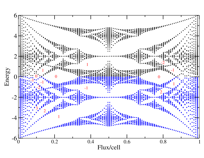
Figure 5: (color online). Weyl loop Hofstadter spectrum of model (11), which has $C=-1$ at zero field. The flux per lattice cell is expressed in units of the flux quantum, $\phi_{0}=h/|e|$. The occupied states for half filling are colored in blue. The Hall conductance values (in units of $e^{2}/h$) in some of the gaps is shown in red.

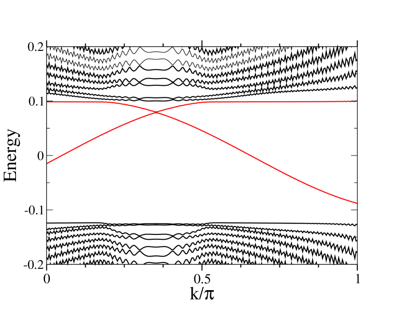
Figure 6: (color online). Spectrum of model (11) for a ribbon geometry under a weak magnetic field flux $\phi/\phi_{0}=1/400$, vs. longitudinal momentum. The edge states are highlighted in red.

At stronger magnetic field, the magnetic length becomes comparable to the lattice spacing and the energy spectrum exhibits the fractal structure known as the Hofstadter butterflyhofstadter . A calculation of Hofstadter butterfly spectra for Weyl nodes in 3D systems has recently been doneRoy . Fig. 5 shows the Hofstadter spectrum for the model (11) with $\mu=2$, $\lambda=-0.1$ and $M=0$, at half-filling. The Fermi energy lies above the gap, for small flux, as the model’s Chern number $C=-1$, in agreement with the above discussion. Quantized Hall conductances (in units of $e^{2}/h$) are also shown in some of the Hofstadter gaps. Although the half-filled system is metallic for small field, it may become an insulator with zero Hall conductance, at higher flux values.

The spectrum for a ribbon geometry is shown in Fig. 6 for the same model, for a small magnetic flux. Fig. 6 confirms the presence of edge states crossing the gap with the predicted chirality. An interesting difference between such a ribbon spectrum for a loop and that of a Hamiltonian with two Dirac pointseu is readily apparent. In the latter, the LL’s dispersion with longitudinal momentum are easily recognizable as plateaus, while in Fig. 6 such LL plateaus are not seen. The reason for this difference lies in the fact that LLs near the loop gap have high order, so that the wave functions $\phi_{n}$ in Eq.(17) contain high order Hermite polynomials. The edge states therefore decay fairly slowly into the bulk and finite size effects (the ribbon’s width) are relatively strong.

IV Conclusion

We studied a minimal Dirac ring Hamiltonian with mass gap terms, for two-dimensional fermions, as a model for a Dirac loop anomalous Hall insulator. We derived and expression for the Chern number which assigns a chirality to the gapped loop through the phase winding of the mass gap terms. The change in the Chern number at a topological transition can also be calculated from a previously introduced index that we generalized to the Dirac loop case.

The Landau level spectrum in a weak magnetic field was shown to depend on the loop’s chirality. The Fermi level has a high LL index. In the case of an anomalous Hall insulator, a weak magnetic field turns the system into a metal, although it may become a trivial insulator at higher fields. In the spinfull case of a topological insulator where spin $s_{z}$ is conserved, the weak magnetic field’s gauge field turns the system into a spin Hall insulator with finite magnetization.

We also studied the Hofstadter butterfly spectrum for arbitrary field, as well as the edge states in a ribbon geometry. The latter decay slower into the bulk and are therefore more sensitive to finite size effects in the Dirac loop case, when compared to the case of Dirac nodes.

A recent proposal for the realization of a Dirac loop semimetal in two dimensions has appeared recentlyLu . We also expect that the models introduced above are suitable for realization in optical lattices.

References

- (1) M.Z.Hasan andC.L.Kane, Rev.Mod. Phys. 82, 3045 (2010).
- (2) X.L. Qi and S.C. Zhang, Rev. Mod. Phys. 83, 1057 (2011).
- (3) A. Altland and M. Zirnbauer, Phys. Rev. B, 55 (1997) 1142; A. P. Schnyder, S. Ryu, A. Furusaki, and A.W.W. Ludwig, Phys. Rev. B 78, 195125 (2008); A. Kitaev, AIP Conf. Proc. 1134, 22 (2009).
- (4) Alicea J., Rep. Prog. Phys. 75 (2012) 076501.
- (5) X. Wan, A. M. Turner, A. Vishwanath, and S.Y. Savrasov, Phys. Rev. B 83, 205101 (2011).
- (6) P. Delplace, J. Li, and D Carpentier, Europhys. Lett. 97, 67004 (2012).
- (7) J-.M. Hou, Phys. Rev. Lett. 111, 130403 (2013).
- (8) S. M. Young and C. L. Kane, Phys. Rev. Lett. 115, 126803 (2015).
- (9) S. Ganeshan and S. D. Sarma, Phys. Rev. B 91, 125438 (2015)
- (10) H. Nielsen and M. Ninomiya, Phys. Lett. B 130, 389 (1983).
- (11) Z. Wang, Y. Sun, X.-Q. Chen, C. Franchini, G. Xu, H. Weng, X. Dai, and Z. Fang, Phys. Rev. B 85, 195320 (2012).
- (12) S.-Y. Xu, C. Liu, S. K. Kushwadha, T.-R. Chang, J. W. Krizan, R. Shankar, C. M. Polley, J. Adell, T. Balasubramanian, K. Miyamoto. N Alidoust, G. Bian, M. Neupane, I. Belopolski, H.-T. Jeng, C.-Y. Huang, W.-F. Tsai, H. Lin, F. C. CHou, T. Okuda, A. Okuda, A. Bansil, R. J. Cava, and M. Z. Hasan, arXiv:1312.7624.
- (13) Z. K. Liu, B. Zhou, Y. Zhang, H. M. Weng, D. Prabhakaran, S.-K. Mo, Z. X. Shen, Z. Fang, X. Dai, Z. Hussain, and Y. L. Chen, Science 343, 864 (2014).
- (14) Z. Wang, H. Weng, Q. Xu, X. Dai, and Z. Fang, Phys. Rev. B 88, 125427 (2013).
- (15) Z. K. Liu, J. Jiang, B. Zhou, Z. J. Wang, Y. Zhang, H. M. Weng, D. Prabhakaran, S.-K. Mo, H. Peng, P. Dudin, T. kim, M. Hoech, Z. Fang, X. Dai, Z. X. Shen, D. L. Feng, Z. Hussain, and Y. L. Chen, Nat. Mater. 13, 677 (2014).
- (16) M. Neupane, S.-Y. Xu, R. Sankar, N. Alidoust, G. Bian, C. Liu, I. Belopolski, T.-R. Chang, H.-T. Jeng, H. Lin, A. Bansil, F. Chou, and M. Z. Hasan, Nat. Commun. 5, 3786 (2014).
- (17) S. Borisenko, Q. Gibson, D. Evtushinsky, V. Zabolotnyy, B. Büchner, and R. J. Cava, Phys. Rev. Lett. 113, 027603 (2014).
- (18) H. Weng, C. Fang, Z. Fang, B. A. Bernevig, and X. Dai, Phys. Rev. X 5, 011029 (2015).
- (19) S.-M. Huang, S.-Y. Xu, I. Belopolski, C.-C. Lee, G. Chang, B. Wang, N. Alidoust, G. Bian, M. Neupane, C. Zhang, S. Jia, A. Bansil, H. Lin, and M. Z. Hasan, Nat. Commun. 6, 7373 (2015).
- (20) S.-Y. Xu, I. Belopolski, N. Alidoust, M. Neupane, G. Bian, C. Zhang, R. Sankar, G. Chang, Z. Yuan, C.-C. Lee, S.-M. Huang, H. Zheng, J. Ma, D. S. Sanchez, B.Wang, A. Bansil, F. Chou, P. P. Shibayev, H. Lin, S. Jia, and M. Z. Hasan, Science 349, 613 (2015).
- (21) B.Q. Lv, H. M. Weng, B. B. Fu, X. P. Wang, H.Miao, J. Ma, P. Richard, X. C. Huang, L. X. Zhao, G. F. Chen, Z. Fang, X. Dai, T. Qian, and H. Ding, Phys. Rev. X 5, 031013 (2015).
- (22) L. X. Yang, Z. K. Liu, Y. Sun, H. Peng, H. F. Yang, T. Zhang, B. Zhou, Y. Zhang, Y. F. Guo, M. Rahn, D. Prabhakaran, Z. Hussain, S.-K. Mo, C. Felser, B. Yan, and Y. L. Chen, Nat. Phys. 11, 728 (2015).
- (23) K. Mullen, B. Uchoa and D. T. Glatzhofer Phys. Rev. Lett. 115, 026403 (2015).
- (24) R. Nandkishore, Phys. Rev. B, 93 020506 (2016).
- (25) Z. Yan and Z. Wang, arXiv:1605.04404.
- (26) J. L. Lu, W. Luo, X. Y. Li, S. Q. Yang, J. X. Cao, X. G. Gong, H. J. Xiang, arXiv:1603.04596
- (27) Proc. R. Soc. London, Ser. A 392, 45 (1984)).
- (28) M. A. N. Araújo and E. V. Castro, J. Phys. Cond. Matter 26, 075501 (2014).
- (29) H. B. Nielsen and M. Ninomiya, Nucl. Phys. B185, 20 (1981).
- (30) L. Li and S. Chen, Phys. Rev. B 92, 085118 (2015).
- (31) T. Fukui, Y. Hatsugai, and H. Suzuki, J. Phys. Soc. Jpn. 74, 1674 (2005).
- (32) X. L. Qi, Y.-S. Wu, and S.-C. Zhang, Phys. Rev. B 74, 085308 (2006).
- (33) F. D. M. Haldane, Phys. Rev. Lett. 61, 2015 (1988).
- (34) N. Goldman, W. Beugeling, and C. Morais Smith, Europhysics Letters 97, 23003 (2012); Phys. Rev. B 86, 075118 (2012).
- (35) C. J. Tabert and E. J. Nicol, Phys. Rev. Lett. 110, 197402 (2013).
- (36) C. L. Kane and E. J. Mele, Phys. Rev. Lett. 95, 146802 (2005).
- (37) D. N. Sheng, Z.Y. Weng, L. Sheng, and F. D. M. Haldane, Phys. Rev. Lett. 97 036808 (2006).
- (38) Xiao-Liang Qi, Yong-Shi Wu, and Shou-Cheng Zhang, Phys. Rev. B 74, 045125 (2006).
- (39) M. Onoda, Y. Avishai, and N. Nagaosa, Phys. Rev. Lett. 98, 076802 (2007).
- (40) D. R. Hofstadter, Phys. Rev. B 14 , 2239 (1976).
- (41) S. Roy, M. Kolodrubetz, J. Moore and A. Grushin, arXiv: 1605.08445 (unpublished).