On the Perturbation-Iteration Algorithm for System of Fractional Differential Equations

Abstract

In this study, perturbation-iteration algorithm, namely PIA, is applied to solve some types of system of fractional differential equations (FDEs) for the first time. To illustrate the efficiency of the method, numerical solutions are compared with the results published in the literature by considering some FDEs. The results confirm that the PIA is powerful, simple and reliable method for solving system of nonlinear fractional differential equations.

Keywords: Fractional-integro differential equations, Caputo fractional derivative, Initial value problems, Perturbation-Iteration Algorithm. AMS 2010: 34A08, 34A12.

1 Introduction

As an important mathematical branch investigating the properties of derivatives and integrals, the history of the fractional calculus is nearly as old as classical integer order analysis. Even though there is a long period of time since the beginning of fractional calculus, it could not find practical applications for many years. However, in last decades, it has found a place in various areas such as control theory, Senol et al. (2014), viscoelasticity, Yu and Lin. (1998), electrochemistry, Oldham (2010) and electromagnetic, Heaviside (2008).

The evolution of the symbolic computation programs such as Matlab and Mathematica is one of the driving forces behind this increased usage. Various multidisciplinary problems could be expressed by the help of fractional derivatives and integrals. For example, in Hamamci, (2007). The most important descriptions of fundamentals of fractional calculus have been studied by Mainardi, (1997) and Podlubny, (1998). Existence and uniqueness of the solutions has also been studied by Yakar and Koksal (2012) and the references therein.

Parallel to the studies in applied sciences, system of fractional differential equations (FDEs) allowed scientists to describe and model various important and useful physical problems.

The number of differential equations whose solution can not be found analytically. That situations appear in FDEs more than the other types of differential equations. In this case, as the study of algorithms using numerical approximation for the problems of mathematical analysis, the field of numerical analysis is used for approximate solutions of FDEs. In recent years, a significant effort has been expended to propose numerical methods for this purpose. These methods include, fractional variational iteration method, Wu and Lee, (2010); Guo and Mei (2011), homotopy perturbation method, Abdulaziz et al. (2008); He (2012); Momani and Odibat, (2007); Zhang et al. (2014) and fractional differential transform method (Momani et al., 2007; Arikoglu and Ozkol, 2009; El-Sayed et al., 2014).

In this study, we have applied the previously developed method PIA to obtain approximate solutions for some system of FDEs. Our method is suitable for a broad class of equations and does not require special assumptions and restrictions.

In the literature, there exists a few fractional derivative definitions of an arbitary order. Two mostly used of them are the Riemann-Liouville and Caputo fractional derivatives. The two definitions are quite similar but have different order of evaluation of derivation.

Riemann-Liouville fractional integration of order $\alpha$ is defined by:

$$J^{\alpha}f(x)=\frac{1}{\Gamma(\alpha)}\int_{0}^{x}(x-t)^{\alpha-1}f(t)dt,\quad\alpha>0,\quad x>0.$$ (1)

The following two equations are defined as Riemann-Liouville and Caputo fractional derivatives of order $\alpha,$ respectively.

$$D^{\alpha}f(x)=\frac{d^{m}}{dx^{m}}\left(J^{m-\alpha}f(x)\right)$$ (2)

$$D_{\ast}^{\alpha}f(x)=J^{m-\alpha}\left(\frac{d^{m}}{dx^{m}}f(x)\right).$$ (3)

where $m-1<\alpha<m$ and $m\in\mathbf{N}.$

Due to the appropriateness of the initial conditions, fractional definition of Caputo is often used in recent years.

Definition 1.1

The fractional derivative of $u(x)$ $in$ the Caputo sense is defined as

$$D_{\ast}^{\alpha}u(x)=\left\{\begin{array}[]{cc}\frac{1}{\Gamma(m-\alpha)}\int_{0}^{x}(x-t)^{m-\alpha-1}u^{(m)}(t)dt&,m-1<\alpha<m\\ \frac{d^{m}}{dx^{m}}&,\alpha=m\end{array}\right.$$ (4)

for $m-1<\alpha<m,$ $m\in\mathbf{N},$ $x>0,$ $u\in C_{-1}^{m}.$

Also, we need here two of its basic properties.

Lemma 1.2

If $m-1<\alpha<m,$ $m\in\mathbf{N}$ and $u\in C_{\mu}^{m},$ $\mu-1$ then

$$D_{\ast}^{\alpha}J^{\alpha}u(x)=u(x)$$ (5)

and

$$J^{\alpha}D_{\ast}^{\alpha}u(x)=u(x)-\sum_{k=0}^{m-1}u^{(k)}(0^{+})\frac{x^{k}}{k!},\quad x>0.$$ (6)

After this introductory section, Section 2 is reserved to a brief review of the Perturbation-Iteration Algorithm PIA(1,1), in Section 3 some examples are presented to show the efficiency and simplicity of the algorithm. Finally the paper ends with a conclusion in Section 4.

2 Overview of the Perturbation-Iteration Algorithm PIA(1,1)

As one of the most practical subjects of physics and mathematics, differential equations create models for a number of problems in science and engineering to give an explanation for a better understanding of the events. Perturbation methods have been used for this purpose for over a century (Nayfeh, 2008; Jordan and Smith, 1987; Skorokhod et al., 2002). These methods could be used to search approximate solutions of integral equations, difference equations, integro-differential equations and partial differential equations.

But the main difficulty in the application of perturbation methods is the requirement of a small parameter or to install a small artificial parameter in the equation. For this reason, the obtained solutions are restricted by a validity range of physical parameters. Therefore, to overcome the disadvantages come with the perturbation techniques, some methods have been suggested by several authors (He, 2001; Mickens, 1987, 2005, 2006; Cooper, 2002; Hu and Xiong, 2003; He, 2012; Wang and He, 2008; Iqbal and Javed, 2011; Iqbal et al., 2010).

Parallel to these studies, recently a new perturbation-iteration algorithm has been proposed by Aksoy, Pakdemirli and their co-workers, Aksoy and Pakdemirli (2010); Pakdemirli et al. (2011); Aksoy et al. (2012). A previous attempt of constructing root finding algorithms systematically, Pakdemirli and Boyacı(2007), Pakdemirli et al. (2007); Pakdemirli et al. (2008). finally guided to generalization of the method to differential equations also Aksoy and Pakdemirli, (2010); Pakdemirli et al. (2011); Aksoy et al. (2012). In the new technique, an iterative algorithm is established on the perturbation expansion. The method has been applied to first order equations Pakdemirli et al. (2011) and Bratu type second order equations, Aksoy and Pakdemirli, (2010) to obtain approximate solutions. Then the algorithms were tested on some nonlinear heat equations also Aksoy et al. (2012). Finally, the solutions of the Volterra and Fredholm type integral equations (Dolapci et al., 2013) and ordinary differential equation and systems, Şenol et al. (2013) have given by the present method.

In this study, the previously developed new technique is applied to some types of nonlinear fractional differential equations for the first time. To obtain the approximate solutions of equations, the most basic perturbation-iteration algorithm PIA(1,1) is employed by taking one correction term in the perturbation expansion and correction terms of only first derivatives in the Taylor series expansion, i.e. $n=1,m=1$.

Consider the following initial value problem.

$$F_{k}\left(D^{\alpha}u_{k},u_{j},\varepsilon,t\right)=0$$ (7)

$$k=1,2,\dots,K$$

$$j=1,2,\dots,K$$

$$u^{(k)}(0)=c_{k},\qquad k=0,1,2,\ldots,m-1,\quad m-1<\alpha\leq m$$ (8)

where $K$ is the number of the equation in the system and $D^{\alpha}$ is the Caputo fractional derivative of order $\alpha$, which is defined by:

$$D^{\alpha}u(t)=J^{m-\alpha}\left(\frac{d^{m}}{dt^{m}u(t)}\right),\quad m-1<\alpha<m,\quad m\in\mathbf{N}$$ (9)

As more clearly the system could be expressed by:

$${F_{1}} {=} F_{1}\left(u_{1}^{\left(\alpha\right)},u_{1},u_{2},{\dots,u}_{k},\varepsilon,t\right)=0$$

$$F_{2} = F_{2}\left(u_{2}^{\left(\alpha\right)},u_{1},u_{2},{\dots,u}_{k},\varepsilon,t\right)=0$$

$$\vdots$$

$$F_{K} = F_{K}\left(u_{k}^{\left(\alpha\right)},u_{1},u_{2},{\dots,u}_{k},\varepsilon,t\right)=0$$ (10)

In this method as $\varepsilon$ is the artificially introduced perturbation parameter and we use only one correction term in the perturbation expansion.

$$u_{k,n+1} = u_{k,n}+\varepsilon(u_{c})_{k,n}$$

$$u_{k,n+1}^{\prime} = u_{k,n}^{\prime}+\varepsilon(u_{c}^{\prime})_{k,n}$$ (11)

where subscript $n$ represents the $n.$iteration

Replacing $(\ref{8})$ into $(\ref{4})$ and writing in the Taylor Series expansion for only first order derivatives in the neighborhood of $\varepsilon=0$ gives

$$F_{K}=\sum_{m=0}^{M}{\frac{1}{m!}{\left[{\left(\frac{d}{d\varepsilon}\right)}^{m}F_{K}\right]}_{\varepsilon=0}^{m}\varepsilon^{m},\ \ \ \ }k=1,2,\dots,K$$ (12)

for

$$\frac{d}{d\varepsilon}=\frac{\partial u_{k,n+1}^{\left(\alpha\right)}}{\partial\varepsilon}\frac{\partial}{\partial u_{k,n+1}^{\left(\alpha\right)}}+\sum_{j=1}^{K}{\left(\frac{\partial u_{j,n+1}}{\partial\varepsilon}\frac{\partial}{\partial u_{j,n+1}}\right)}+\frac{\partial}{\partial\varepsilon}$$ (13)

This equation is defined for the $(n+1).$iteration equation

$$F_{k}\left(u_{k,n+1}^{\left(\alpha\right)},u_{j,n+1},\varepsilon,t\right)=0$$ (14)

Replacing $(\ref{10})$ in $(\ref{9})$ yields our iteration equation:

$$F_{K}=\sum_{m=0}^{M}\frac{1}{m!}{\left[{\left(\frac{{\left((u_{c})_{k,n}\right)}^{\left(\alpha\right)}}{\partial\varepsilon}\frac{\partial}{\partial u_{k,n+1}^{\left(\alpha\right)}}+\sum_{j=1}^{K}(u_{c})_{j,n}{\frac{\partial}{\partial u_{j,n+1}}}+\frac{\partial}{\partial\varepsilon}\right)}^{m}F_{K}\right]}_{\varepsilon=0}^{m}\varepsilon^{m}=0,$$ (15)

$$k=1,2,\dots,K$$

All derivatives are calculated at $\varepsilon=0.$

Beginning with an initial function $u_{0}$, first $(u_{c})_{k,n}$ ’s has been determined by the help of $(\ref{12})$. Then using Eq. $(\ref{8})$, $\left(n+1\right).$ iteration solution could be found Iteration process is repeated using $(\ref{12})$ and $(\ref{8})$ until achieving an acceptable result.

3 Application

Example 3.1

Consider the following system of linear fractional differential equations Abdulaziz et al. 2008:

$$D^{\alpha}u_{1}\left(t\right) = u_{1}\left(t\right)+u_{2}\left(t\right)$$

$$D^{\beta}u_{1}\left(t\right){\ } = -u_{1}\left(t\right)+u_{2}\left(t\right)$$ (16)

$$0<\alpha,\beta\leq 1$$

given with the initial conditions $u_{1}\left(0\right)=0$ and$\ \ u_{2}(0)=1$. The known exact solutions for $\alpha=\beta=1$ are

$$u_{1}\left(t\right)=e^{t}sint$$ (17)

and

$$u_{2}(t)=e^{t}cost$$ (18)

Eq. $(\ref{13})$ can be rearranged in the following form with adding and subtracting $u_{1,n}^{\prime}(t)$ and $u_{2,n}^{\prime}(t)$ to the equation:

$$\varepsilon\frac{d^{\alpha}u_{1}(t)}{{dt}^{\alpha}}+u_{1,n}^{\prime}\left(t\right)-\varepsilon u_{1,n}^{\prime}\left(t\right)-\varepsilon u_{1,n}\left(t\right)-\varepsilon u_{2,n}\left(t\right)=0$$ (19)

$$\varepsilon\frac{d^{\beta}u_{2}(t)}{{dt}^{\beta}}+u_{2,n}^{{}^{\prime}}\left(t\right)-\varepsilon u_{2,n}^{{}^{\prime}}\left(t\right)+\varepsilon u_{1,n}\left(t\right)-\varepsilon u_{2,n}\left(t\right)=0$$ (20)

where $\varepsilon$ is a small parameter. According to the iteration formula for

$$F\left(u_{1}^{{}^{\prime}},u_{1},\varepsilon\right)=\frac{1}{\Gamma(1-\alpha)}\varepsilon\int_{0}^{t}{\frac{u_{1}^{\prime}(s)}{{(t-s)}^{\alpha}}ds+u_{1,n}^{{}^{\prime}}\left(t\right)-\varepsilon u_{1,n}^{{}^{\prime}}\left(t\right)-\varepsilon u_{1,n}\left(t\right)-\varepsilon u_{2,n}\left(t\right)}$$ (21)

$$F\left(u_{2}^{{}^{\prime}},u_{2},\varepsilon\right)=\frac{1}{\Gamma(1-\beta)}\varepsilon\int_{0}^{t}{\frac{u_{2}^{\prime}(s)}{{(t-s)}^{\beta}}ds+u_{2,n}^{{}^{\prime}}\left(t\right)-\varepsilon u_{2,n}^{{}^{\prime}}\left(t\right)+\varepsilon u_{1,n}\left(t\right)-\varepsilon u_{2,n}\left(t\right)}$$ (22)

terms in equation $(\ref{12})$ become

$$F = u_{1,n}^{{}^{\prime}}\left(t\right),\quad F_{u_{1}}=0,\quad F_{u_{1}^{\prime}}=1,$$

$$F_{\varepsilon} = -u_{1,n}^{\prime}\left(t\right)-u_{1,n}\left(t\right)-u_{2,n}\left(t\right)+\frac{1}{\Gamma(1-\alpha)}\int_{0}^{t}{\frac{u_{1,n}^{\prime}\left(s\right)}{{(t-s)}^{\alpha}}ds}$$ (23)

for the iteration formula

$$u_{1}^{{}^{\prime}}\left(t\right)+\frac{F_{u_{1}}}{F_{u_{1}^{\prime}}}u_{1}\left(t\right)=-\frac{F_{\varepsilon}+\frac{F}{\varepsilon}}{Fu_{1}^{\prime}}$$ (24)

and terms in equation $(\ref{12})$

$$F = u_{2,n}^{\prime}\left(t\right),\quad F_{u_{2}}=0,\quad F_{u_{2}^{\prime}}=1,$$

$$F_{\varepsilon} = -u_{2,n}^{{}^{\prime}}\left(t\right)+u_{1,n}\left(t\right)-u_{2,n}\left(t\right)+\frac{1}{\Gamma(1-\beta)}\int_{0}^{t}{\frac{u_{2,n}^{\prime}\left(s\right)}{{(t-s)}^{\beta}}ds}$$ (25)

for the iteration formula

$$u_{2}^{{}^{\prime}}\left(t\right)+\frac{F_{u_{2}}}{F_{u_{2}^{{}^{\prime}}}}u_{2}\left(t\right)=-\frac{F_{\varepsilon}+\frac{F}{\varepsilon}}{F_{u_{2}^{\prime}}}$$ (26)

Notice that inserting the small parameter $\varepsilon$ as a coefficient of the integral term simplifies the system and makes it easy to solve.

After writing these terms in the iteration formulas, the system gives the following differential equations.

$$u_{1,n}\left(t\right)+u_{2,n}\left(t\right)+\frac{(-1+\varepsilon)u_{1},{{}_{n}}^{{}^{\prime}}(t)}{\varepsilon}=\frac{1}{\Gamma\left(1-\alpha\right)}\int_{0}^{t}{\frac{u_{1,n}^{{}^{\prime}}\left(s\right)}{{\left(t-s\right)}^{\alpha}}ds+}({u_{c})_{1,n}^{\prime}(t)}$$ (27)

and

$${-}u_{1,n}\left(t\right)+u_{2,n}\left(t\right)+\frac{(-1+\varepsilon)u_{2,n}^{{}^{\prime}}(t)}{\varepsilon}=\frac{1}{\Gamma\left(1-\beta\right)}\int_{0}^{t}{\frac{u_{2,n}^{{}^{\prime}}\left(s\right)}{{\left(t-s\right)}^{\beta}}ds+}({u_{c})_{2,n}^{\prime}(t)}$$ (28)

When employing the iteration formula $(\ref{12})$, we start with an initial function compatible to the boundary condition and we determine coefficients from the boundary condition at each step. Beginning with the initial functions

$$u_{1,0}\left(t\right)=0~{}\text{ and }~{}u_{2,0}\left(t\right)=1$$

and using the iteration formula, we get the following successive approximate solutions at each step for $n=0,1,2,\dots$

$$u_{1,1}\left(t\right) = t$$

$$u_{2,1}\left(t\right) = 1+t$$

$$u_{1,2}\left(t\right) = t\left(2+t-\frac{t^{1-\alpha}}{\Gamma(3-\alpha)}\right)$$

$$u_{2,2}\left(t\right) = 1+2t-\frac{t^{2-\beta}}{\Gamma(3-\beta)}$$

$$u_{1,3}\left(t\right) = \frac{1}{3}t\left(9+t(9+t)+\frac{3t^{2-2\alpha}}{\Gamma\left(4-2\alpha\right)}-\frac{9t^{1-\alpha}(3+t-\alpha)}{\Gamma\left(4-\alpha\right)}-\frac{3t^{2-\beta}}{\Gamma\left(4-\beta\right)}\right)$$

$$u_{2,3}\left(t\right) = 1+3t-\frac{t^{3}}{3}+\frac{t^{3-\alpha}}{\Gamma\left(4-\alpha\right)}+t^{2-2\beta}\left(\frac{t}{\Gamma\left(4-2\beta\right)}-\frac{t^{\beta}\left(9+t-3\beta\right)}{\Gamma\left(4-\beta\right)}\right)$$ (29)

and so on. Following in this manner the fifth iteration solutions $u_{1,5}(t)$ and $u_{2,5}(t)$ were calculated. Due to brevity reasons, higher iterations are not given here. It is easy to calculate other iterations up to any order by the help of a symbolic calculation software such as Mathematica . In Figure 1. and 2. we compare our $u_{1,5}(t)$ and $u_{2,5}(t)$ solutions for different values of $\alpha$ and $\beta$ and in Figure 3. and 4. with the exact solution graphically. In Table 1. and 2. some of our iterations are compared with the exact solution. The results show that the proposed method can give successful approximations.

Table 1: Numerical results of Example 1. for some values of $u_{1}(t)$.

$\alpha=\beta=1$
$t$	$u_{1,1}(t)$	$u_{1,2}(t)$	$u_{1,3}(t)$	$u_{1,4}(t)$	$u_{1,5}(t)$	$Exact$ $Solution$	$Absolute$ $Error$
0.0	0.000000	0.000000	0.000000	0.000000	0.000000	0.000000	0.000000
0.1	0.100000	0.110000	0.110333	0.110333	0.110332	0.110332	1.12698E-8
0.2	0.200000	0.240000	0.242666	0.242666	0.242656	0.242655	7.31405E-7
0.3	0.300000	0.390000	0.399000	0.399000	0.398919	0.398910	8.44622E-6
0.4	0.400000	0.559999	0.581333	0.581333	0.580991	0.580943	0.00004809
0.5	0.500000	0.750000	0.791666	0.791666	0.790625	0.790439	0.00018591
0.6	0.600000	0.960000	1.032000	1.031999	1.029408	1.028845	0.00056233
0.7	0.700000	0.190000	1.304333	1.304333	1.298731	1.297295	0.00143589
0.8	0.800000	1.440000	1.610666	1.610666	1.599744	1.596505	0.00323866
0.9	0.900000	1.710000	1.953000	1.952999	1.933316	1.926673	0.00664370
1.0	1.000000	2.000000	2.333333	2.333333	2.300000	2.287355	0.01264471

Table 2: Numerical results of Example 1. for some values of $u_{2}(t)$.

$\alpha=\beta=1$
$t$	$u_{2,1}(t)$	$u_{2,2}(t)$	$u_{2,3}(t)$	$u_{2,4}(t)$	$u_{2,5}(t)$	$Exact$ $Solution$	$Absolute$ $Error$
0.0	1.000000	1.000000	1.000000	1.000000	1.000000	1.000000	0.00000000
0.1	1.100000	1.099999	1.099666	1.099650	1.099649	1.099649	1.6274E-10
0.2	1.200000	1.200000	1.197333	1.197066	1.197055	1.197056	2.13559E-8
0.3	1.300000	1.300000	1.291000	1.289650	1.289568	1.289569	3.74045E-7
0.4	1.400000	1.400000	1.378666	1.374399	1.374058	1.374061	2.87222E-6
0.5	1.500000	1.500000	1.458333	1.447916	1.446874	1.446889	0.00001403
0.6	1.600000	1.600000	1.528000	1.506399	1.503807	1.503859	0.00005154
0.7	1.700000	1.700000	1.585666	1.545650	1.540047	1.540803	0.00015535
0.8	1.800000	1.800000	1.629333	1.561066	1.550144	1.550549	0.00040529
0.9	1.900000	1.900000	1.659999	1.547650	1.527966	1.528913	0.00094681
1.0	2.000000	2.000000	1.666666	1.500000	1.466666	1.468693	0.00202727

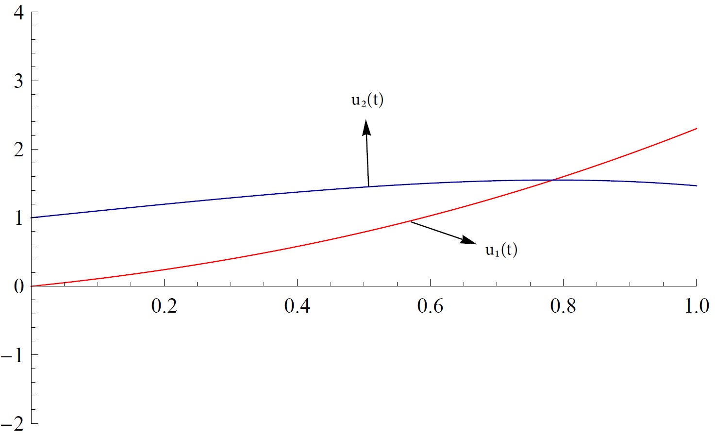
Figure 1: Comprasion of the $u_{1,5}(t)$ and $u_{2,5}(t)$ of Example 1. for $\alpha=\beta=1$.

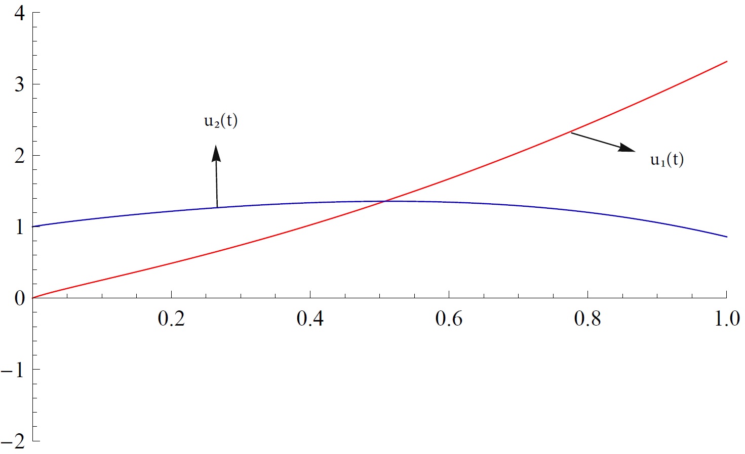
Figure 2: Comprasion of the $u_{1,5}(t)$ and $u_{2,5}(t)$ of Example 1. for $\alpha=0.7$ and $\beta=0.9$.

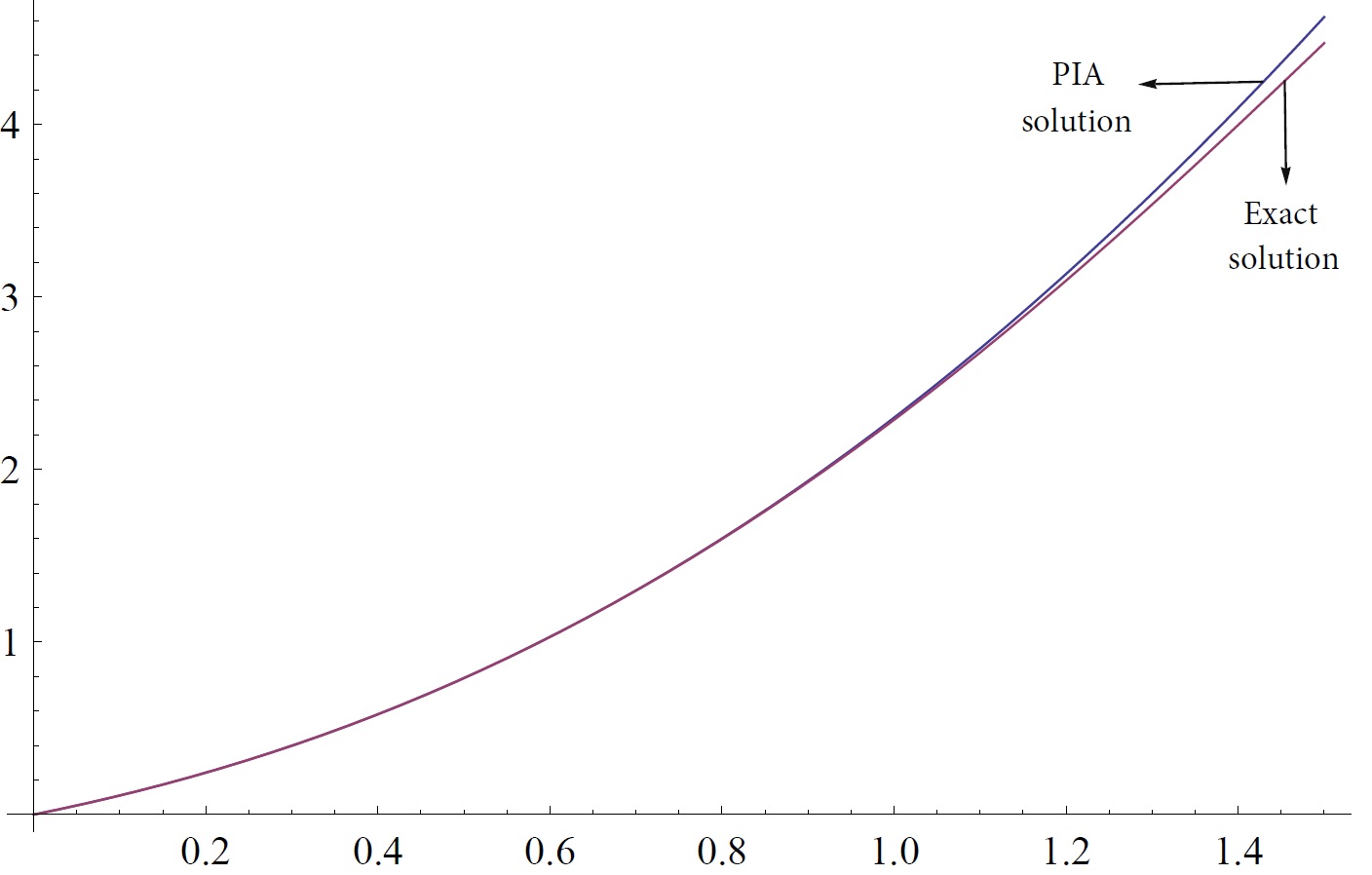
Figure 3: Comprasion of the exact solution and the PIA solution $u_{1,5}(t)$ of Example 1. for $\alpha=\beta=1$.

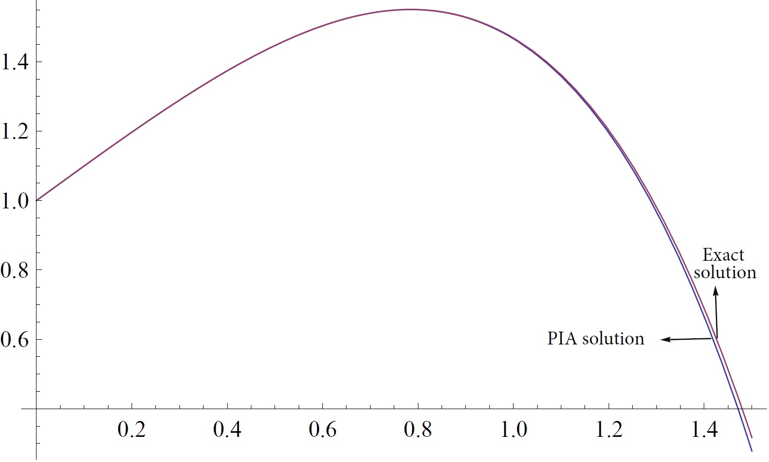
Figure 4: Comprasion of the exact solution and the PIA solution $u_{2,5}(t)$ of Example 1. for $\alpha=\beta=1$.

Example 3.2

For the second example consider the following system of nonlinear fractional differential equations Zurigat et al. 2010:

$$D^{\alpha_{1}}{u}_{1}{\left(t\right)\ } = \frac{1}{2}{u}_{1}\left(t\right)$$

$$D^{\alpha_{2}}u_{2}{\left(t\right)\ } = u_{2}\left(t\right)+{u}_{1}^{2}{\left(t\right)}$$ (30)

$$0<\alpha_{1},\alpha_{2}\leq 1$$

given with the initial conditions ${u}_{1}\left(0\right)=1$ and$\ u_{2}(0)=0$. The exact solutions, when $\alpha_{1}=\alpha_{2}=1$, are

$${u}_{1}\left(t\right)=e^{\frac{t}{2}}$$ (31)

and

$$u_{2}(t)={te}^{t}$$ (32)

In the system, if add and subtract $u_{1,n}^{\prime}(t)$ and $u_{2,n}^{\prime}(t)$ respectively, the system could be rewritten in the following form:

$$\varepsilon D^{\alpha_{1}}{u}_{1}{\left(t\right)\ \ }+{u}_{1,n}^{\prime}\left(t\right)-\varepsilon{u}_{1,n}^{\prime}\left(t\right)-\frac{1}{2}\varepsilon{u}_{1,n}\left(t\right)=0$$ (33)

$$\varepsilon D^{\alpha_{2}}u_{2}{\left(t\right)\ }+u_{2,n}^{\prime}\left(t\right)-\varepsilon u_{2,n}^{\prime}\left(t\right)-\varepsilon u_{2,n}\left(t\right)-\varepsilon{u}_{1,n}^{2}\left(t\right){\ }=0$$ (34)

where $\varepsilon$ is a small parameter. For

$$F\left({u}_{1}^{{}^{\prime}},{u}_{1},\varepsilon\right)=\frac{1}{\Gamma(1-\alpha_{1})}\varepsilon\int_{0}^{t}{\frac{{u}_{1,n}^{\prime}(s)}{{(t-s)}^{\alpha_{1}}}ds+{u}_{1,n}^{\prime}(t)-\varepsilon{u}_{1,n}^{\prime}(t)-\frac{1}{2}\varepsilon{u}_{1,n}\left(t\right)}$$ (35)

$$F\left(u_{2}^{{}^{\prime}},u_{2},\varepsilon\right)=\frac{1}{\Gamma(1-\alpha_{2})}\varepsilon\int_{0}^{t}{\frac{u_{2,n}^{\prime}(s)}{{(t-s)}^{\alpha_{2}}}ds+{u}_{2,n}^{\prime}(t)-\varepsilon{u}_{2,n}^{\prime}(t)-\varepsilon u_{2,n}\left(t\right)-\varepsilon{u}_{1,n}^{2}{\left(t\right)}}$$ (36)

and terms in equation $(\ref{12})$ become

$$F = {u}_{1,n}^{\prime}(t),\quad F_{{u}_{1}}=0,\quad F_{{u}_{1}^{\prime}}=1,$$

$$F_{\varepsilon} = -{u}_{1,n}^{\prime}(t)-\frac{{u}_{1,n}(t)}{2}+\frac{1}{\Gamma(1-\alpha_{1})}\int_{0}^{t}{\frac{{u}_{1,n}^{\prime}(t)}{{(t-s)}^{\alpha_{1}}}ds}$$ (37)

and

$$F = u_{2,n}^{\prime}(t),\quad F_{u_{2}}=0,\quad F_{u_{2}^{\prime}}=1,$$

$$F_{\varepsilon} = -u_{2,n}^{\prime}(t)-u_{2,n}(t)-{u}_{1,}^{2}{{}_{n}}(t)+\frac{1}{\Gamma(1-\alpha_{2})}\int_{0}^{t}{\frac{u_{2,n}^{\prime}(s)}{{(t-s)}^{\alpha_{2}}}ds}$$ (38)

After writing these terms in the iteration formula we obtain the following differential equations:

$$2\left(\frac{\int_{0}^{t}{{(-s+t)}^{-\alpha_{1}}{u}_{1,n}^{\prime}(s)ds}}{\Gamma(1-\alpha_{1})}+({u_{c})_{1,n}^{\prime}(t)}-\frac{(-1+\varepsilon){({u}_{1,n})}^{{}^{\prime}}(t)}{\varepsilon}\right)={u}_{1,n}\left(t\right)$$ (39)

and

$$u_{2,n}\left(t\right)+u_{1,n}^{2}{\left(t\right)}+\frac{\left(-1+\varepsilon\right){\left(u_{2,n}\right)}^{{}^{\prime}}\left(t\right)}{\varepsilon}=\frac{\int_{0}^{t}{{(-s+t)}^{-\alpha_{2}}{(u_{2,n})}^{{}^{\prime}}s)ds}}{\Gamma(1-\alpha_{2})}+({u_{c})_{2,n}^{\prime}(t)}$$ (40)

Beginning with the initial functions

$${u}_{1,0}\left(t\right)=1~{}\text{and}~{}u_{2,0}\left(t\right)=0$$

and using the iteration formula, the following successive approximate solutions are obtained for $n=0,1,2,\dots$

$$u_{1,1}(t) = 1+\frac{t}{2}$$

$$u_{2,1}(t) = t$$

$$u_{1,2}(t) = \frac{1}{8}\left(8+8t+t^{2}+\frac{4t^{2-\alpha_{1}}}{\Gamma(2-\alpha_{1})(-2+\alpha_{1})}\right)$$

$$u_{2,2}\left(t\right) = 2t+t^{2}+\frac{t^{3}}{12}+\frac{t^{2-\alpha_{2}}}{\Gamma(2-\alpha_{2})\left(-2+\alpha_{2}\right)}$$

$$u_{1,3}\left(t\right) = \frac{1}{48}\left(48+72t+18t^{2}+t^{3}+\frac{24t^{3-2\alpha_{1}}}{\Gamma(4-2\alpha_{1})}-\frac{24t^{2-\alpha_{1}}\left(9+t-3\alpha_{1}\right)}{\Gamma(4-\alpha_{1})}\right)$$

$$u_{2,3}\left(t\right) = 3t+3t^{2}+\frac{5t^{3}}{6}+\frac{t^{4}}{12}+\frac{t^{5}}{320}+\frac{t^{3-2\alpha_{2}}}{\Gamma(4-2\alpha_{2})}-\frac{t^{5-2\alpha_{1}}}{4\Gamma{(3-\alpha_{1})}^{2}\left(-5+2\alpha_{1}\right)}$$ (41)

$$-\frac{t^{3-\alpha_{1}}\left(4\left(40+3t\left(10+t\right)\right)+\alpha_{1}\left(-72-t\left(64+7t\right)+\left(8+t\left(8+t\right)\right)\alpha_{1}\right)\right)}{8\Gamma\left(6-\alpha_{1}\right)}$$

$$-\frac{t^{2-\alpha_{2}}(72+t(24+t)+6\alpha_{2}(-7-t+\alpha_{2}))}{2\Gamma(5-\alpha_{2})}$$

and so on. In the same manner the fourth iteration solutions $u_{1,4}(t)$ and $u_{2,4}(t)$ are calculated. Again we compared our results In Figures 5., 6., 7. and 8. and in Table 3. and 4. with the exact solutions.

Table 3: Numerical results of Example 2. for some values of $u_{1}(t)$.

$\alpha_{1}=\alpha_{2}=1$
$t$	$u_{1,1}(t)$	$u_{1,2}(t)$	$u_{1,3}(t)$	$u_{1,4}(t)$	$Exact$ $Solution$	$Absolute$ $Error$
0.0	1.000000	1.000000	1.000000	1.000000	1.000000	0.0000000
0.1	1.050000	1.051250	1.051270	1.051271	1.051271	2.6260E-9
0.2	1.100000	1.105000	1.105166	1.105170	1.105170	8.4742E-8
0.3	1.150000	1.161250	1.161812	1.161833	1.161834	6.4897E-7
0.4	1.200000	1.220000	1.221333	1.221400	1.221402	2.7581E-6
0.5	1.250000	1.281250	1.283854	1.284016	1.284025	8.4896E-6
0.6	1.300000	1.345000	1.349500	1.349837	1.349858	0.0000213
0.7	1.350000	1.411250	1.418395	1.419021	1.419067	0.0000464
0.8	1.400000	1.480000	1.490666	1.491733	1.491824	0.0000913
0.9	1.450000	1.551250	1.566437	1.568146	1.568312	0.0001660
1.0	1.500000	1.625000	1.645833	1.648437	1.648721	0.0002837

Table 4: Numerical results of Example 2. for some values of $u_{2}(t)$.

$\alpha_{1}=\alpha_{2}=1$
$t$	$u_{2,1}(t)$	$u_{2,2}(t)$	$u_{2,3}(t)$	$u_{2,4}(t)$	$Exact$ $Solution$	$Absolute$ $Error$
0.0	0.000000	0.000000	0.000000	0.000000	0.000000	0.0000000
0.1	0.100000	0.110083	0.110505	0.110516	0.110517	2.4666E-7
0.2	0.200000	0.240666	0.244084	0.244272	0.244280	8.12862-6
0.3	0.300000	0.392250	0.403929	0.404894	0.404957	0.0000635
0.4	0.400000	0.565333	0.593365	0.596453	0.596729	0.0002760
0.5	0.500000	0.760416	0.815852	0.823492	0.824360	0.0008683
0.6	0.600000	0.978000	1.074993	1.091043	1.0932712	0.0022277
0.7	0.700000	1.218583	1.374530	1.404661	1.409626	0.0049654
0.8	0.800000	1.482666	1.718357	1.770446	1.780432	0.0099863
0.9	0.900000	1.770750	2.110517	2.195074	2.213642	0.0185684
1.0	1.000000	2.083333	2.555208	2.685825	2.718281	0.0324559

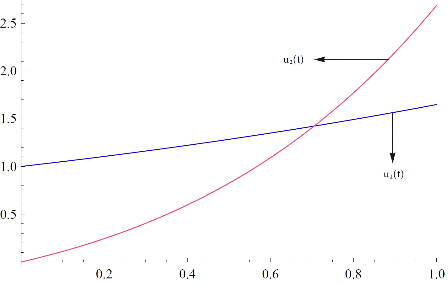
Figure 5: Comprasion of the $u_{1,4}(t)$ and $u_{2,4}(t)$ of Example 2. for $\alpha_{1}=\alpha_{2}=1$.

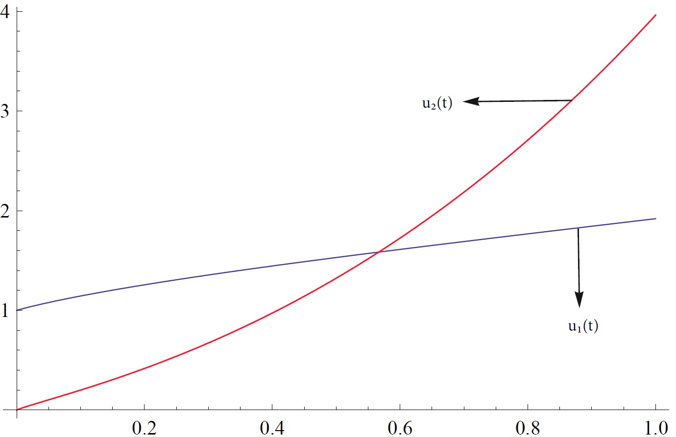
Figure 6: Comprasion of the $u_{1,4}(t)$ and $u_{2,4}(t)$ of Example 2. for $\alpha_{1}=0.5$ and $\alpha_{2}=0.8$.

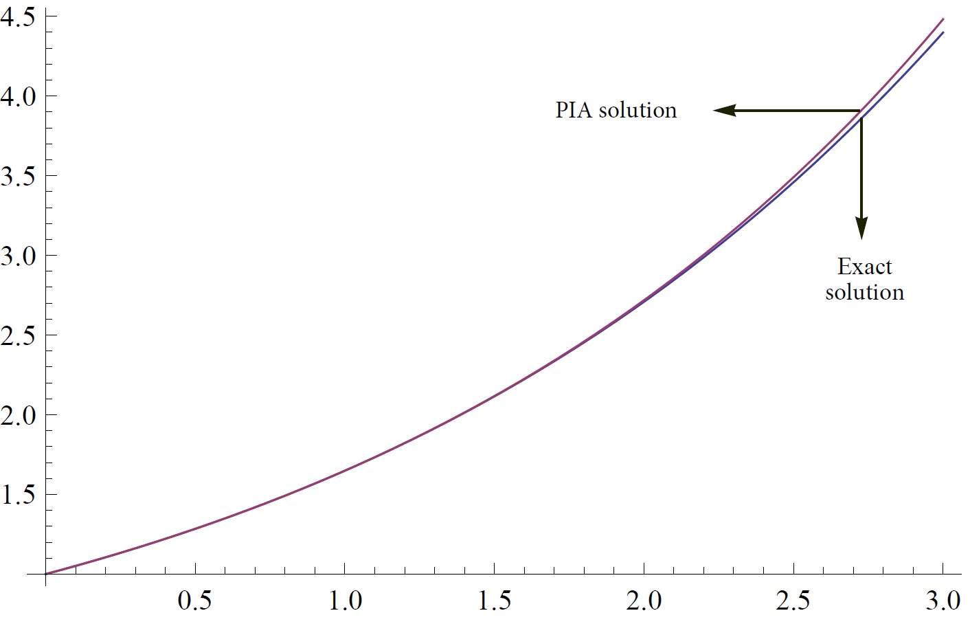
Figure 7: Comprasion of the exact solution and the PIA solution $u_{1,4}(t)$ of Example 2. for $\alpha_{1}=\alpha_{2}=1$.

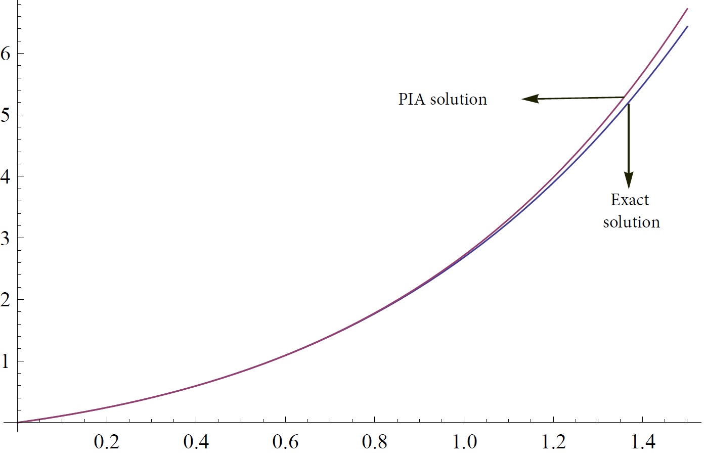
Figure 8: Comprasion of the exact solution and the PIA solution $u_{2,4}(t)$ of Example 2. for $\alpha_{1}=\alpha_{2}=1$.

4 Conclusion

In this paper we have applied previously developed numerical method so-called Perturbation-Iteration Algorithm (PIA) to find approximate solutions of some system of nonlinear Factional Differential Equations for the first time. The numerical results obtained in this study show that method PIA is a remarkably successful numerical technique for solving system of FDEs. We expect that the present method could used to calculate the approximate solutions of other types of fractional differential equations such as fractional integro-differential equations and fractional partial differential equations. Our next study will be about these types of equations.

5 Authors’ contributions

All authors contributed in development of the manuscript and solving problems. All authors read and approved the final manuscript.

6 Competing interests

The authors declare that they have no competing interest.

References

- [1] Abdulaziz O, Hashim I, Momani S (2008) Solving systems of fractional differential equations by homotopy-perturbation method. Physics Letters A 372 (4):451-459
- [2] Aksoy Y, Pakdemirli M (2010) New perturbation-iteration solutions for Bratu-type equations Computers & Mathematics with Applications 59:2802-2808
- [3] Aksoy Y, Pakdemirli M, Abbasbandy S, Boyaci H (2012) New perturbation-iteration solutions for nonlinear heat transfer equations International Journal of Numerical Methods for Heat & Fluid Flow 22:814-828
- [4] Arikoglu A, Ozkol I (2009) Solution of fractional integro-differential equations by using fractional differential transform method Chaos, Solitons & Fractals 40:521-529
- [5] Cooper K, Mickens R (2002) Generalized harmonic balance/numerical method for determining analytical approximations to the periodic solutions of the x 4/3 potential Journal of Sound and Vibration 250:951-954
- [6] Dolapci İT., Şenol M, Pakdemirli M (2013) New perturbation iteration solutions for Fredholm and Volterra integral equations Journal of Applied Mathematics 2013
- [7] El-Sayed A, Nour H, Raslan W, El-Shazly E (2014) A study of projectile motion in a quadratic resistant medium via fractional differential transform method Applied Mathematical Modelling
- [8] Filobello-Nino U et al. (2013) Laplace transform-homotopy perturbation method as a powerful tool to solve nonlinear problems with boundary conditions defined on finite intervals Computational and Applied Mathematics:1-16
- [9] Guo S, Mei L (2011) The fractional variational iteration method using He’s polynomials Physics Letters A 375:309-313
- [10] Hamamci SE (2007) An algorithm for stabilization of fractional-order time delay systems using fractional-order PID controllers Automatic Control, IEEE Transactions on 52:1964-1969
- [11] He JH Homotopy perturbation method with an auxiliary term. In: Abstract and Applied Analysis, 2012. Hindawi Publishing Corporation,
- [12] He JH (2001) Iteration Perturbation Method for Strongly Nonlinear Oscillators J Sound Vibr 7:631-642
- [13] Heaviside O (2008) Electromagnetic theory vol 3. Cosimo, Inc.,
- [14] Hu H, Xiong Z-G (2003) Oscillations in an x(2m+2)/(2n+1) potential Journal of Sound and Vibration 259:977-980
- [15] Iqbal S, Idrees M, Siddiqui AM, Ansari A (2010) Some solutions of the linear and nonlinear Klein–Gordon equations using the optimal homotopy asymptotic method Applied mathematics and computation 216:2898-2909
- [16] Iqbal S, Javed A (2011) Application of optimal homotopy asymptotic method for the analytic solution of singular Lane–Emden type equation Applied Mathematics and Computation 217:7753-7761
- [17] Jafari H, Yousefi S, Firoozjaee M, Momani S, Khalique CM (2011) Application of Legendre wavelets for solving fractional differential equations Computers & Mathematics with Applications 62:1038-1045
- [18] Jordan DW, Smith P, Smith P (1987) Nonlinear ordinary differential equations
- [19] Mainardi F (1997) Fractals and fractional calculus in continuum mechanics. vol 378. Springer Verlag,
- [20] Mickens R (1987) Iteration procedure for determining approximate solutions to non-linear oscillator equations Journal of Sound and Vibration 116:185-187
- [21] Mickens R (2006) Iteration method solutions for conservative and limit-cycle x1/3 force oscillators Journal of Sound and Vibration 292:964-968
- [22] Mickens R (2005) A generalized iteration procedure for calculating approximations to periodic solutions of “truly nonlinear oscillators” Journal of Sound and Vibration 287:1045-1051
- [23] Momani S, Odibat Z (2007) Homotopy perturbation method for nonlinear partial differential equations of fractional order Physics Letters A 365:345-350
- [24] Momani S, Odibat Z, Erturk VS (2007) Generalized differential transform method for solving a space-and time-fractional diffusion-wave equation Physics Letters A 370:379-387
- [25] Nayfeh AH (2008) Perturbation methods. John Wiley & Sons,
- [26] Oldham KB (2010) Fractional differential equations in electrochemistry Adv Eng Softw 41:9-12 doi:DOI 10.1016/j.advengsoft.2008.12.012
- [27] Pakdemirli M, Aksoy Y, Boyacı H (2011) A New Perturbation-Iteration Approach for First Order Differential Equations Mathematical and Computational Applications 16:890-899
- [28] Pakdemirli M, Boyacı H (2007) Generation of root finding algorithms via perturbation theory and some formulas Applied Mathematics and Computation 184:783-788
- [29] Pakdemirli M, Boyaci H, Yurtsever H (2007) Perturbative derivation and comparisons of root-finding algorithms with fourth order derivatives Mathematical and Computational Applications 12:117
- [30] Pakdemirli M, Boyaci H, Yurtsever H (2008) A root-finding algorithm with fifth order derivatives Mathematical and Computational Applications 13:123
- [31] Podlubny I (1998) Fractional differential equations: an introduction to fractional derivatives, fractional differential equations, to methods of their solution and some of their applications vol 198. Academic press,
- [32] Senol B, Ates A, Baykant Alagoz B, Yeroglu C (2014) A numerical investigation for robust stability of fractional-order uncertain systems ISA Transactions 53:189-198
- [33] Skorokhod AV, Hoppensteadt FC, Salehi HD (2002) Random perturbation methods with applications in science and engineering vol 150. Springer Science & Business Media,
- [34] Şenol M, Timuçin Dolapci İ, Aksoy Y, Pakdemirli M Perturbation-Iteration Method for First-Order Differential Equations and Systems. In: Abstract and Applied Analysis, 2013. Hindawi Publishing Corporation,
- [35] Wang S-Q, He J-H (2008) Nonlinear oscillator with discontinuity by parameter-expansion method Chaos, Solitons & Fractals 35:688-691
- [36] Wu G-c, Lee E (2010) Fractional variational iteration method and its application Physics Letters A 374:2506-2509
- [37] Yakar A, Koksal ME Existence results for solutions of nonlinear fractional differential equations. In: Abstract and Applied Analysis, 2012. Hindawi Publishing Corporation,
- [38] Yu ZS, Lin JZ (1998) Numerical research on the coherent structure in the viscoelastic second-order mixing layers Appl Math Mech-Engl 19:717-723
- [39] Zhang X, Zhao J, Liu J, Tang B (2014) Homotopy perturbation method for two dimensional time-fractional wave equation Applied Mathematical Modelling 38:5545-5552
- [40] Zurigat M, Momani S, Odibat Z, Alawneh A (2010) The homotopy analysis method for handling systems of fractional differential equations. Applied Mathematical Modelling 34 (1):24-35