Stereo Video Deblurring

Abstract

Videos acquired in low-light conditions often exhibit motion blur, which depends on the motion of the objects relative to the camera. This is not only visually unpleasing, but can hamper further processing. With this paper we are the first to show how the availability of stereo video can aid the challenging video deblurring task. We leverage 3D scene flow, which can be estimated robustly even under adverse conditions. We go beyond simply determining the object motion in two ways: First, we show how a piecewise rigid 3D scene flow representation allows to induce accurate blur kernels via local homographies. Second, we exploit the estimated motion boundaries of the 3D scene flow to mitigate ringing artifacts using an iterative weighting scheme. Being aware of 3D object motion, our approach can deal robustly with an arbitrary number of independently moving objects. We demonstrate its benefit over state-of-the-art video deblurring using quantitative and qualitative experiments on rendered scenes and real videos.

1 Introduction

Stereo is one of the oldest areas of computer vision research [1]. Interestingly, the arrival of mass-produced active depth sensors [2] seems to have renewed interest also in passive stereo systems. In contrast to active depth sensors, stereo cameras are also applicable in outdoor environments. Due to their more general applicability, stereo cameras are gaining increased adoption, for example in autonomous driving [3]. Remarkably, the availability of stereo image pairs also helps in the estimation of temporal correspondences: On the KITTI optical flow benchmark [4], the best performing algorithms [5, 6] are indeed scene flow algorithms that jointly estimate depth and 3D motion from stereo videos. Part of their advantage stems from an increased robustness to adverse imaging conditions [6]. One such adverse imaging condition is a shortage of light. In low-light conditions, the exposure time often needs to be increased to obtain a reasonable signal-to-noise-ratio. But when either the camera, or the objects in the scenes are moving during exposure time, this results in motion blurred images.

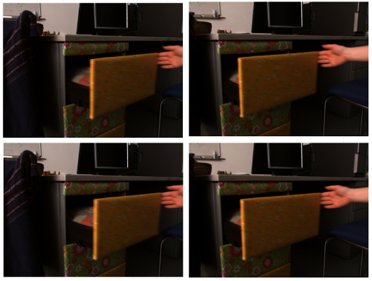
(a) Input

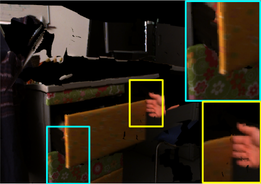
(b) Blurry 3D point cloud

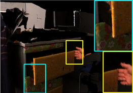
(c) Deblurred 3D point cloud

Figure 1: Application of stereo video deblurring: Given 2 consecutive stereo frames LABEL:sub@fig:teaser:input, our deblurring approach allows to estimate sharp textures from stereo video input with motion blur. Rendering scene flow geometry with the blurred input image as a colored point-cloud from a new point of view produces an unnatural motion blur LABEL:sub@teaser:blurry. Our stereo video deblurring algorithm can remove the blur LABEL:sub@teaser:sharp

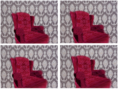
(a) Input: 2 stereo frames

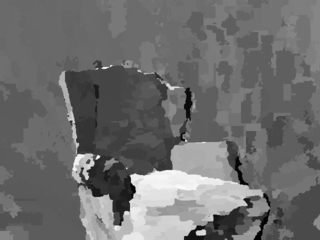
(b) Over-segmentation

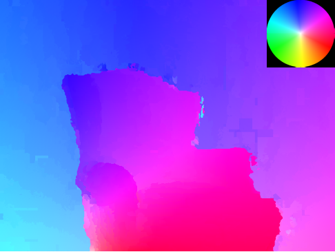
(c) Optical flow

(d) Optical flow deblurring

(e) Ours

(f) Video deblurring [7]

Figure 2: Stereo video deblurring: For two consecutive frames of a synthetic stereo video LABEL:sub@fig:sceneFlow:input we use the scene flow approach of Vogel et al. [6] to compute an over-segmentation into planar patches with constant 3D rigid body motion LABEL:sub@fig:sceneFlow:overseg. Projecting the 3D motion onto the image plane yields optical flow LABEL:sub@fig:sceneFlow:OF, which our baseline algorithm uses to deblur a reference frame LABEL:sub@fig:sceneFlow:2DSF. Exploiting the homographies from the 3D motion and object boundary information from the over-segmentation, our full approach obtains sharp images avoiding ringing and boundary artifacts LABEL:sub@fig:sceneFlow:3DSF. Our result is also clearly sharper than state-of-the-art video deblurring [7] LABEL:sub@fig:sceneFlow:Kim

Motion blur is not only unsatisfactory to look at, it can also disturb further image-based processing, e. g. in tasks such as panorama stitching [8] or barcode recognition [9]. In stereo video setups, viewpoint-dependent motion blur hinders a post-capture adjustment of the baseline, the acquisition and visualization of 3D point clouds (see Fig. 1 for an example) or the controll of tele-operated robots in the presence of rapid robot and/or object motion.

In this paper we address the challenge of deblurring stereo videos. In contrast to the substantial literature on removing camera shake [10, 11, 12, 13, 14, 15], we aim to deal with the more general case of camera and object motion. In case of independent motions, mixed pixels at motion boundaries yield significant complications. Removing such spatially-variant blur is extremely challenging when attempted from single images [16, 17], but video input helps to significantly increase robustness [7, 18]. Unlike previous work, we leverage stereo video to obtain substantially improved and more robust deblurring results. In our approach, we exploit 3D scene flow in various ways and make the following contributions: (i) We show that 3D scene flow can improve video deblurring by providing more accurate motion estimates. In particular, we exploit piecewise rigid scene flow [6], which yields an over-segmentation of the image into planar patches that move with a rigid 3D motion (Figs. 2b and 2c). (ii) We demonstrate that the resulting piecewise homographies allow to directly induce blur matrices. Thereby, we take into account that the projection of a rigid 3D motion yields non-linear motion trajectories in 2D (Fig. 3, Tab. 3). We find that this leads to superior deblurring results compared to inducing the blur matrices from an optical flow field [7] (Figs.2d to 2f). (iii) We apply the homography-induced blur matrices in a robust deblurring procedure that attenuates the effects of motion discontinuities using an iterative weighting scheme; Initial motion discontinuities are obtained from 3D scene flow. We demonstrate the superiority of the proposed stereo video deblurring over state-of-the-art monocular video deblurring using experiments on synthetic data as well as on real videos.

2 Related Work

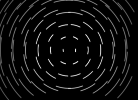
(a) Homography-induced blur

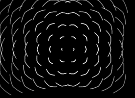
(b) Optical flow-induced blur

(c) Difference of blurs

Figure 3: Descriptiveness of homography-based blur kernels: Using 3D rigid body motion to generate blur kernels, we can faithfully express, e. g., yaw motion LABEL:sub@fig:kernel:rotHom, while kernels constructed with spatially varying 2D displacement vectors fields [7] only yield an approximation LABEL:sub@fig:kernel:rotFlow. Approximation errors LABEL:sub@fig:kernel:rotDiff are also present close to the rotation axis where motions are small (extremly large yaw angle and all intensities scaled for better visibility)

The goal of this work is to obtain sharp images from stereo videos containing 3D camera and object motion. Of course, in principle blind deblurring could be applied to each frame individually. However, blind motion deblurring from a single image is a highly underconstrained problem, as blur parameters and sharp image have to be estimated from a single measurement. To cope with spatially-variant blur due to the 3D motion of the camera, single image deblurring approaches frequently use homographies [19, 20, 21]. In contrast, we apply homographies to describe spatially-variant object motion blur. Single image object motion deblurring approaches keep the number of parameters manageable by either choosing the motion of a region from a very restricted set of spatially-invariant box filters [22, 23], assuming it to have a spatially-invariant, non-parametric kernel of limited size [16], or to be representable by a discrete set of basis kernels [24]. Approaches that rely on learning spatially-variant blur are also limited to a discretized set of detectable motions [17, 25]. Kim et al. [26] consider continuously varying box filters for every pixel, but rely heavily on regularization.

Connecting deblurring and depth estimation, Xu and Jia [27] successfully apply stereo correspondence estimation to motion-blurred stereo frames to support blind image deblurring. Lee and Lee [28], Arun et al. [29], and Hu et al. [30] estimate sharp images and depth jointly. However, all these approaches assume the scene to be static and camera motion to be the only source of motion blur.

Cho et al. [31] deblur images of independently moving objects. The multiple input images of their algorithm are unordered, and a piecewise affine registration between the images, as well as the motion underlying the blur, has to be estimated. To restrict the parameter space, the blur kernels are assumed to be piecewise constant and linear.

Video deblurring approaches reduce the number of parameters through the assumption that the inter-frame and intra-frame motion are related by the duty cycle of the camera. He et al. [32] and Deng et al. [33] apply feature tracking of a single moving object to obtain 2D displacement-based blur kernels for deblurring. Wulff and Black [18] refine the latter approach and perform segmentation into two layers, estimation of the affine motion parameters, as well as deblurring of each layer jointly. Relaxing the assumption of two layers and affine motion, Yamaguchi et al. [34] and Kim and Lee [7] employ optical flow to approximate spatially variant blur kernels for deblurring. Yamaguchi et al. [34] propose deblurring based on the flow estimates from the blurry images. Kim and Lee [7] iteratively refine flow estimation and deblurred video frames by minimizing a joint energy. The latter method represents the state-of-the-art in video deblurring and is used for comparison in the experimental section. To the best of our knowledge, exploiting stereo video for deblurring has not been considered in the literature before.

Correspondence estimation on stereo video sequences can be improved by estimating stereo correspondences and optical flow jointly as 3D scene flow [35, 36, 37]. In our approach we build on the piecewise rigid scene flow by Vogel et al. [6] for the following reasons. First, it provides us with explicit 3D rotations and translations that we employ for accurate blur kernel construction. Second, through over-segmentation into planar patches, it also delivers occlusion information, which we use as initialization for our boundary-aware object motion deblurring. A general problem in object motion deblurring is that object boundaries with mixed foreground and background pixels can lead to severe ringing artifacts (see Fig. 2). Explicit segmentation and $\alpha$-matting [18, 38] can prevent this effect, but requires restrictive assumptions on the number of moving objects. To handle general scenes with an arbitrary number of objects, we extend the robust outlier handling of Chen et al. [39] to spatially-variant deblurring based on scene flow, and apply it to the mixed pixels at object boundaries.

In contrast to the aforementioned deblurring approaches, Cho et al. [40] deblur hand-held video under the assumption that patches are sharp in some frames of the video. However, in the case of autonomous robots or objects passing the field of view with high speed, this assumption does not hold. Joshi et al. [41] attach additional inertial measurement units to the camera, but this does not account for object motion. An additional low-resolution, high frame-rate camera can provide complex motion kernels [38], but does not provide depth estimates in the way a stereo camera can.

3 Blurred Image Formation in Stereo Video

Inducing blur matrices from 3D rigid object motions.

Due to the finite exposure time $\tau$ of our stereo video camera, each frame of each camera is blurred. Our goal is to find a sharp image $I_{t_{0}}$ for a reference camera at time $t_{0}$. We base our approach on the scene flow of Vogel et al. [6], and likewise assume that the scene can be approximated with planar patches that undergo a 3D rigid body motion. If an object in the scene is non-planar, this assumption leads to an over-segmentation of the object into spatially adjacent patches (see Fig. 2b). Considering video frames where the exposure time is naturally limited by the frame rate, we additionally assume that the motion of each patch is constant during the exposure time of two consecutive frames. Note that a constant rigid motion in 3D does not necessarily imply that its 2D projection is constant; the projection may, e. g. in the case of a rotation, be constantly accelerated. However, our assumption excludes rapidly changing motions such as vibrations.

Constant 3D rigid body motion can be expressed as a homogeneous $4\times 4$ matrix

$$M=\begin{pmatrix}R&T\\ \vec{0}&1\end{pmatrix}$$ (1)

with a rotation matrix $R\in\mathbb{R}^{3\times 3}$ and a translation vector $T\in\mathbb{R}^{3}$. To enable our highly accurate blur kernel description, we rewrite $M=\exp\big{(}\theta\xi\big{)}$ as matrix exponential, where $\theta\in\mathbb{R}$ describes the rotation angle and $\xi$ is a $4\times 4$ matrix that is determined by the rotation axis and the translation, see [42, 43]. With $M$ describing the motion between time instants $t_{0}$ and $t_{1}$, the constant 3D motion between two arbitrary time instants $t_{a}$ and $t_{b}$ is given as

$$M_{t_{b},t_{a}}=\exp\left(\frac{t_{b}-t_{a}}{t_{1}-t_{0}}\theta\xi\right).$$ (2)

In a piecewise planar scene approximation, the 3D planes of the patches at time $t$ are defined via their scaled normals $n_{t}$. All points $P$ on the plane satisfy the equation $P^{\text{T}}n_{t}=1$, where $P^{\text{T}}$ is the transposed of $P$. We can relate a moving 3D point to its corresponding pixel location on the image plane via the camera geometry. Given the calibration matrix $K$ of the reference camera and its location $T_{K}$, the projection from a 3D plane to the image plane at time $t$ can be written in homogeneous coordinates as $Pr_{t}=K-KT_{K}n_{t}^{\text{T}}$, see e. g. [6].

Under the assumption of color constancy, two sharp images of the reference camera (with hypothetical infinitesimal exposure) at different times are connected via

$$I_{t_{a}}(x)=I_{t_{b}}(\prescript{t_{b}}{}{H}^{t_{a}}x)\quad\text{where}\quad\prescript{t_{b}}{}{H}^{t_{a}}=Pr_{t_{b}}M_{t_{b},t_{a}}Pr_{t_{a}}^{-1}.$$ (3)

With this notation, a blurry image pixel $x$ in the interior of a patch is formed from the reference image as

$$\hat{B}(x)=\int^{t_{0}+\frac{\tau}{2}}_{t_{0}-\frac{\tau}{2}}I_{t}(x)\,\text{d}t=\int^{t_{0}+\frac{\tau}{2}}_{t_{0}-\frac{\tau}{2}}I_{t_{0}}(\prescript{t_{0}}{}{H}^{t}x)\,\text{d}t,$$ (4)

where

$$\prescript{t_{0}}{}{H}^{t}=Pr_{t_{0}}\exp\big{(}-t\theta\xi\big{)}Pr_{t}^{-1}$$ (5)

is a homography that can be computed exactly from camera geometry, normal, and motion. To put it differently, a 3D point that is projected to $x$ on the image plane describes a certain trajectory on the image plane during the exposure time. If the 3D point follows a rigid body motion, the homography $\big{(}\prescript{t_{0}}{}{H}^{t}\big{)}^{-1}$ allows us to exactly describe this 2D trajectory. In contrast, optical flow based methods [7, 24, 44], employ 2D optical flow vectors to generate $I_{t}$ via forward warping. Thus the trajectory of a point on the image plane is approximated by a 2D line that is traversed with constant velocity. As optical flow is spatially variant, the trajectories may change for each pixel, hence induce blur kernels with a curved shape. However, more complex motions such as rotations can only be approximated, Fig. 3. In our approach, the description of trajectories due to 3D rigid body motions is exact. As our experiments show, this also results in more faithfully deblurred images.

By discretizing the integration over time with $\delta t=\frac{\tau}{N}$ (we fix $N=70$) and using bilinear image interpolation, we can obtain a discretized version of Eq. (4) for vectorized reference images as $\hat{B}(x)=A_{x}\vec{I}_{t_{0}}$. Here, $A_{x}$ denotes a sparse row vector that depends on the homography estimated at pixel $x$. Stacking the blur vectors $A_{x}$ for each pixel, we obtain our homography-based blur matrix $A$ leading to $\hat{\vec{B}}=A\vec{I}_{t_{0}}$.

Table 1: Overview of the different sources of motion information used for video deblurring: When pure 2D correspondence is considered (top two rows), the induced blur kernels are only approximate, as motion trajectories are assumed to be linear. Exploiting homographies from scene flow allows us to capture the fact that rigid 3D object motion leads to non-linear trajectories

o @lX[1,c]X[1,c]X[1.2,c]@			linear approximation
Motion information	# of frames	# of views	of trajectories
optical flow	2	1	yes
2D projection of scene flow	2	2	yes
homographies	2	2	no

Motion boundaries.

If only scene points from the same plane contribute to the color $B(x)$ of the measured blurred image at point $x$, the image formation model of Eq. (4) is exact. If at time $t$ a scene point with a different motion contributes to $B(x)$ we should also use the corresponding homography. However, within an object, the planar patches are adjacent in space and move consistently. Therefore, we approximate the blur with the row vector $A_{x}$ induced by the homography of $x$ at $t_{0}$. At motion boundaries, the homographies are very different and as pixels of foreground and background mix, transparency effects occur. While such effects can be modeled, taking them into account requires precise localization of the motion boundaries, which is very challenging. Instead, we exclude motion boundaries from the deblurring process by means of an iterative approach. In each iteration, we downweight pixels with a high difference between image formation model and measured image and try to find a sharp image that explains the remaining pixels. Under the assumption of additive Gaussian noise, we use the residual to compute a weight for each pixel as

$$w_{n}(x)=\exp\Big{(}-k_{\sigma}\|B(x)-A_{x}\vec{I}^{n-1}_{t_{0}}\|^{2}\Big{)},$$ (6)

where $\vec{I}^{n-1}_{t_{0}}$ denotes the current estimate of the sharp (color) image. For normalized images we set $k_{\sigma}=\nicefrac{{4000}}{{3}}$ as default value. In the first iteration we initialize $w_{0}$ with the binary occlusion information from the scene flow. As Fig. 4 shows, the weights converge quickly. Some pixels in the image that were initially suppressed as motion boundaries are included in deblurring at a later iteration. More importantly, other pixels where the image formation model is invalid are suppressed later on, which helps controlling ringing artifacts. Suppression may also happen due to some inaccuracies in the computed scene flow. In the experimental section, we will see how this property actually helps to improve deblurring results.

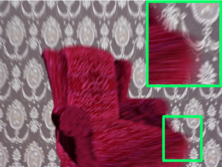
(a) Input

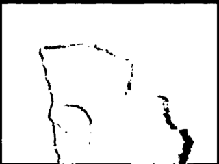
(b) Initial

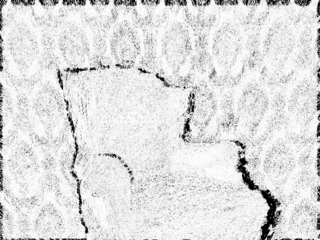
(c) Iteration 3

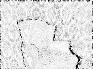
(d) Iteration 10

Figure 4: Downweighting of mixed pixels due to motion boundaries: Foreground and background mix at motion boundaries and violate our image formation model LABEL:sub@fig:occlusion:chair. At motion boundaries and locations of inaccurate flow estimates, the image formation model is downweighed to avoid ringing artifacts. We initialize these weights with the occlusion information provided by the scene flow LABEL:sub@fig:occlusion:init and refine them iteratively LABEL:sub@fig:occlusion:mid,LABEL:sub@fig:occlusion:final

Deblurring.

Theoretically, we could fill in the regions at motion boundaries during deblurring by using adjacent frames or information from the other camera. However, we found experimentally that correspondence estimation in these regions is too unreliable to produce visually pleasing results. Instead, we exploit that natural, sharp images follow a Laplacian distribution of their gradients [22]. In locations where the image formation model is unreliable, e. g., at motion boundaries, we rely on this prior to provide the necessary regularization. Specifically, we obtain an estimate of the sharp reference frame by minimizing the energy

$$E(\vec{I}_{t_{0}})=\sum_{x\in\Omega}\Big{\|}w_{n}(x)\big{(}B(x)-A_{x}\vec{I}_{t_{0}}\big{)}\Big{\|}^{2}+\alpha\rho\big{(}\nabla I_{t_{0}}(x)\big{)},$$ (7)

where $\Omega\subset\mathbb{N}^{2}$ is the image domain and the constant $\alpha$ is fixed to $0.001$. Following prior work [22], we use the robust norm $\rho\big{(}c\big{)}=|c|^{0.8}$ for each color channel and gradient direction.

To solve the optimization problem in Eq. (7), we use iteratively reweighted least squares (IRLS) [45]. In each reweighting iteration, we compute the following weights

$$\rho_{n}(c)=\frac{1}{c}\frac{d\rho\big{(}c\big{)}}{dc}\approx\max\big{(}|c|,\epsilon\big{)}^{0.8-2}\quad\text{ with }\quad\epsilon=0.01$$ (8)

for the smoothness term using the preceding image estimate $\nabla I^{n-1}_{t_{0}}$. Then we minimize the least squares energy

$$E(\vec{I}_{t_{0}},n)=\sum_{x\in\Omega}\big{\|}w_{n}(x)\big{(}B(x)-A_{x}\vec{I}^{n}_{t_{0}}\big{)}\big{\|}^{2}+\alpha\|\rho_{n}\nabla I^{n}_{t_{0}}(x)\|^{2}$$ (9)

via conjugate gradients. We alternate between updating the occlusion weight $w_{n}$ and the smoothness weight $\rho_{n}$. In all our experiments the weights converge quickly and only a few ($\approx 10$) iterations were needed in total.

To compute the 3D scene flow needed for our stereo video deblurring approach, we rely on the method of Vogel et al. [6]. The algorithm is originally designed for sharp images. However, its data term uses the census transform for comparing the warped images, which makes it quite robust to image blur. Of course, scene flow estimation will reach its limits for very strong motion blur. Experimentally, we find that by aggregating evidence in piecewise planar patches, the method yields a scene flow accuracy that turns out to work well in deblurring stereo videos of casual motion. As the following experiments will show, it is crucial, however, to not only rely on the robust correspondence information, but to exploit the homographies to directly induce the blur kernels.

4 Experiments

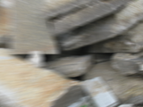
(a) Input

(b) PSNR $30.03$

(c) Difference (b) to
reference image

(d) PSNR $31.02$

(e) Difference (d) to
reference image

Figure 5: Deblurring planar textures: For a planar texture blurred with 3D rigid body motion LABEL:sub@fig:planar:input, deblurring with 2D spatially-variant ground truth displacements LABEL:sub@fig:planar:GT yields ringing errors LABEL:sub@fig:planar:GTdiff that can be reduced by deblurring with our homography-based image formation model LABEL:sub@fig:planar:3SF, LABEL:sub@fig:planar:3SFdiff

(a) Input

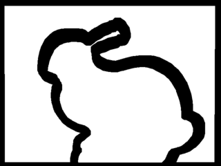
(b) Mask

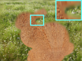
(d) Masked deblurring

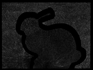
(e) Difference (d) to (f) on (b)

(f) Sharp reference image

Figure 6: Deblurring with masked discontinuities: Our raytraced stereo video frames contain independent object motion of non-planar objects LABEL:sub@fig:saveMask:input. Through the estimated disparity we can assess the shape of the objects LABEL:sub@fig:saveMask:disp. Excluding given discontinuities LABEL:sub@fig:saveMask:mask from the computation of the data term, invalid areas are filled in smoothly LABEL:sub@fig:saveMask:3DSF. The masked difference image LABEL:sub@fig:saveMask:3SFdiff to the real sharp image LABEL:sub@fig:saveMask:GTimg shows that homography-based deblurring has about the same error in planar as in curved surfaces, showing the effectiveness of the over-segmentation from the scene flow

To demonstrate the efficacy of the proposed stereo video deblurring, we perform experiments on synthetic images with known ground truth, as well as on real images. We capture the real video footage with a Point Grey Bumblebee2 stereo color camera, which can acquire $640\times 480$ images at a frame rate of $20$ Hz. We use the internal calibration and supplied software to obtain rectified and demosaiced images. The exposure time of each image can be obtained from the camera software.

In all experiments, we compute scene flow using the publicly available implementation of [6]. We take the default parameters and scale them uniformly to account for the baseline difference between our stereo camera and the KITTI dataset [4] for which they were tuned. For the $640\times 480$ image in Fig. 2 our approach requires $73\text{\,}\mathrm{s}$ to form the discretized blur matrix $A$. Using MATLAB to optimize Eq. (7) in $25$ conjugate gradient steps and $10$ IRLS iterations requires $69\text{\,}\mathrm{s}$ on an $8$-core $4\text{\,}\mathrm{GHz}$ CPU.

Table 2: Deblurring without considering motion-discontinuity regions: For different motions of a planar texture (top) and moving 3D objects with masked object boundaries (bottom), we report the peak signal-to-noise ratio (PSNR) of the deblurred reference frame, the average endpoint error of the estimated motion (AEP), and the average disparity error (ADE) of the estimation. For all scenes the use of scene flow increases deblurring accuracy compared to using optical flow. For scenes with non-fronto-parallel motion (all except ‘upward’ and ‘apples’) homography-based object motion deblurring provides the best results (bold)

blur kernel	ground truth	initial optical		2D projection		3D
source	2D displacement	flow [46]		of scene flow		homographies
	PSNR	AEP	PSNR	AEP	PSNR	ADE	PSNR
upward	26.09	2.53	24.89	0.20	25.83	3.66	25.94
forward	34.12	0.09	34.45	0.10	34.55	0.19	34.74
forward + yaw	30.03	0.15	29.90	0.15	29.95	0.45	31.02
apples	34.36	0.48	29.39	0.81	34.74	4.95	33.33
bunny	25.01	0.62	24.87	0.54	25.09	0.50	25.19
chair	24.84	0.59	23.86	0.47	24.81	0.25	25.03
squares	25.97	2.32	22.69	0.97	25.82	0.65	27.21
triplane	27.43	1.16	27.11	0.49	27.27	0.12	28.30

4.1 Comparing flow-based deblurring to homography-based deblurring

We begin by applying the proposed stereo video deblurring to scenes without object discontinuities. In this way we can analyze the benefit of the homography-induced motion blur model in isolation. We create synthetic sequences by simulating various 3D motions (upward and forward translation, and a combination forward translation and yaw) of a planar, roughly fronto-parallel texture, see Fig. 4a. A second test set consists of rigidly moving 3D objects rendered with a raytracer at very small time steps and averaged to give motion-blurred images (see Figs. 3a, 5a and 6a for the first image of the left view). We take the central frame of each motion-blurred image as a sharp reference frame. For the rendered scenes motion discontinuities are known. In the first experiment, we disable the data term around any motion discontinuities by fixing the weights $w_{n}$ in these areas to zero, see Fig. 5b for an example. As the image prior stays active, the boundaries are filled in smoothly as illustrated in Fig. 5d.

We compare our homography-induced deblurring approach against deblurring with blur matrices generated from different 2D displacement fields. We use forward and backward 2D motion as described by Kim and Lee [7] and apply them in our IRLS deblurring framework. In particular, we use the known ground truth 2D displacement, the 2D initial optical flow with which the scene flow is initialized [46] ( baseline deblurring ), and the 2D projection of the scene flow to induce blur kernels. Table 3 summarizes these settings. Table 2 shows the peak-signal-to-noise-ratio (PSNR) of the deblurred images from the different methods. We observe that the PSNR of our homography-based stereo video deblurring outperforms the results of deblurring with ground truth 2D displacement in all cases of non-fronto-parallel motion. In these cases linear motion trajectories of constant velocity are an approximation. Blur matrices induced by homographies are more expressive and improve the results. Already, deblurring with the 2D projection of scene flow achieves a consistently higher PSNR than deblurring with the initial flow. Indeed, in the case of forward motion, also deblurring with the 2D projection of the scene flow outperforms deblurring with ground truth displacement. The estimated 2D displacement appears to be a better approximation to the linear, but accelerated trajectory of the 3D forward motion than the 2D ground truth displacement. Figs. 4b and 4d show examples of deblurred images using the ground-truth 2D displacement and our homography-based approach. From the difference image between the results and the original sharp texture, Figs. 4c and 4e, we observe that the increase in PSNR is due to the mitigation of ringing effects throughout the image.

For the raytraced scenes the geometry of the moving objects is non-planar and the planarity assumption in our image formation model becomes an approximation. Fig. 3 shows the estimated disparity of an object and the deblurred image obtained by masking out discontinuities. Looking at the difference image, Fig. 5e, we observe that the deblurring error for slightly curved surfaces is comparable to the performance on planar regions of the background, showing that the over-segmentation aids coping with curved surfaces.

For all rendered scenes where the disparity does not exhibit gross errors, we observe in Table 2 that 3D homography-based deblurring improves the PSNR clearly over any form of 2D deblurring. In the scene ‘apples’, Fig. 6a, 1st row, depth estimation fails with a mean disparity error of $4.95$ pixels. In this situation the deblurring quality of homography-based deblurring drops below that of its 2D projection. Still, both outperform the results obtained with the initial optical flow. More importantly, as we will see below, the iterative weighting scheme for treating motion discontinuities can address such disparity estimation errors as well and lead to much improved results.

apples

bunny

squares

triplane

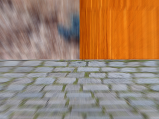
(a) Input

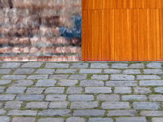
(b) Ours (no boundary downweighting)

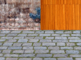
(c) Ours (full)

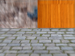
(d) Kim and Lee [7]

Figure 7: Raytraced scenes for evaluating object motion deblurring: The input images exhibit blur due to 3D object motion LABEL:sub@fig:ray:input. Also when 3D homographies are used to induce blur kernels, mixed pixels at object boundaries cause some ringing artifacts LABEL:sub@fig:ray:3Dall. Iteratively downweighting the boundaries from the data term, our full stereo video deblurring LABEL:sub@fig:ray:3SF suppresses ringing and obtains considerably sharper images than state-of-the-art video deblurring LABEL:sub@fig:ray:kim. Please zoom in for detail

4.2 Full algorithm with motion discontinuities

Table 3: Deblurring with motion discontinuities: PSNR of deblurred synthetic scenes with motion discontinuities (top) and real scenes with the camera moving on a motorized rail (bottom). Our homography-based stereo video deblurring with motion boundary weighting (full) clearly outperforms monocular video deblurring with optical-flow induced blur kernels in all cases

	initial optical	2D projection	3D	ours
	flow [46]	of scene flow	homographies	(full)	Kim and Lee [7]
apples	20.89	29.43	26.00	29.48	26.14
bunny	20.72	22.36	22.95	23.20	21.93
chair	19.03	21.57	22.19	23.36	21.78
squares	19.60	21.90	22.56	24.58	22.99
triplane	24.73	24.55	25.22	26.59	23.30
bottles	29.51	29.55	30.80	31.07	28.33
office	31.37	30.87	32.45	32.56	29.01
planar	30.71	31.21	32.33	32.82	30.01
toys	33.51	33.64	34.89	34.90	31.06

We now evaluate the performance of stereo video deblurring in the presence of object motion boundaries. We use the raytraced scenes from the previous experiment, but this time without providing ground-truth information on the motion discontinuities, Fig. 6a. Additionally, we use real images captured with a stereo camera attached to a motorized rail, Fig. 7a. The camera moves forward very slowly on the rail while we capture frames with maximal exposure time and frame rate. By averaging the frames, we obtain motion-blurred images. Comparison to the central frame of the averaged frame series allows for numerical evaluation. Finally, we capture scenes with arbitrarily moving objects for which only a visual evaluation is possible, Fig. 8a. As before we compare against 2D versions of our algorithm. Additionally, we compare against the state-of-the-art video deblurring algorithm of Kim and Lee [7] that uses $3$ consecutive monocular frames. We tuned their regularization parameter to obtain the most accurate results.

In Fig. 6b and Fig. 6c we first contrast homography-induced deblurring without and with handling of motion boundaries. When not taking into account motion boundaries explicitly, i. e. $w_{n}\equiv 1$, Fig. 6b, considerable ringing artifacts are the result, but they are successfully suppressed with our proposed iterative weighting scheme, Fig. 6c. This also becomes evident in the numerical evaluation when comparing the 3 and 4 column of Tab. 3 (top) . For the real sequences in Fig. 3, boundary artifacts are generally less pronounced, as all objects in the scene are static and the camera moves toward the scene. However, as shown in Fig. 4, the discontinuity weight can still compensate errors in scene flow computation. One such example is the erroneous depth estimation in the ‘apples’ scene, which is disabled by the discontinuity weight. Similarly, also in the scenes with the motorized rail, our full object motion deblurring approach improves the PSNR compared to the basic homography approach, Tab. 3 (bottom).

When comparing to the state-of-the-art video deblurring method of Kim and Lee [7], we find that our stereo video deblurring approach yields significantly fewer ringing artifacts and considerably sharper results. This can be seen visually, comparing (d) to (c) of Figs. 3 to 3, as well as quantitatively in Table 3. Interestingly, we find in Table 3 that IRLS deblurring with the 2D projection of the scene flow is already on par with video deblurring of Kim and Lee. 3D homography-based deblurring without boundary handling improves on these result numerically already, highlighting the importance of our homography-induced blur kernels. Yet, our full homography-based object deblurring with motion boundary handling gives further numerical gains and a large visual improvement. Recall that the motion boundaries are initially obtained from the 3D scene flow, thus unique to our setting.

For the real scenes with independent object motion, Fig. 3, we observe that the optical flow-based approaches introduce ringing artifacts, particularly where strong gradients of the background coincide with the object boundary. Our stereo video deblurring algorithm can cope with this situation even in the presence of non-planar, non-rigidly moving objects such as the trousers (2 row) are present.

bottles q

office q

planar

toys

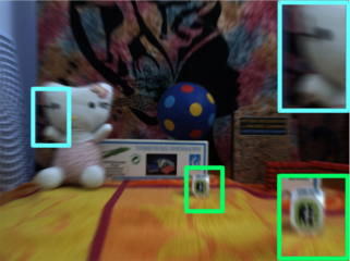
(a) Input

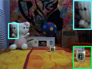
(b) Baseline

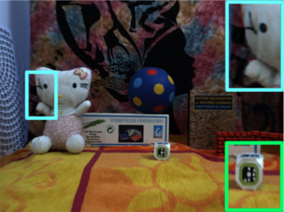
(c) Ours (full)

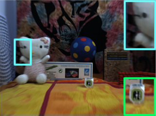
(d) Kim and Lee [7]

Figure 8: Controlled camera motion for evaluating object motion deblurring: Our 3D deblurring LABEL:sub@fig:avrg:3SF has less ringing artifacts than baseline deblurring with optical flow LABEL:sub@fig:avrg:TVAll, and sharper results than video deblurring LABEL:sub@fig:avrg:kim, in particular at the periphery of the images where motion is large

(a) Input

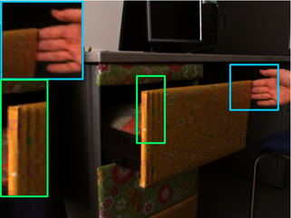
(b) Baseline

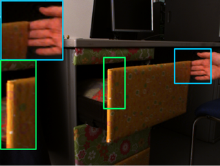
(c) Ours (full)

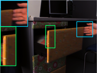
(d) Kim and Lee[7]

Figure 9: For real scenes with independent object motion LABEL:sub@fig:real:input, our novel stereo video deblurring approach LABEL:sub@fig:real:3SF generates fewer ringing artifacts due to object boundaries than baseline deblurring with optical flow LABEL:sub@fig:real:TVAll and sharper images than video deblurring LABEL:sub@fig:real:kim

5 Conclusions and Future Work

We have proposed the first stereo video deblurring approach, which is based on an image formation model that exploits 3D scene flow computed from stereo video. For scenes with an arbitrary number of moving objects, we use an over-segmentation of the scene into planar patches to establish spatially-variant blur matrices based on local homographies. Our experiments on synthetic scenes and real videos show that deblurring with these homographies is more accurate than baseline methods based on 2D linear motion approximations, as well as the current state-of-the-art in video deblurring. Combined with our robust treatment of motion boundaries through an iterative weighting scheme, our approach obtains superior results also on real stereo videos with independently moving objects. In future work we would like to improve the performance of scene flow computation at motion boundaries such that we can benefit from another view to supply information near motion boundaries.

Acknowledgements.

The research leading to these results has received funding from the European Research Council under the European Union’s Seventh Framework Programme (FP7/2007 - 2013) / ERC Grant Agreement No. 307942 and under the European Union’s Horizon 2020 research and innovation programme / ERC Grant Agreement No. 647769.

Stereo Video Deblurring

Anita Sellent Carsten Rother Stefan Roth

F Details on Homography-Based Blur Kernels

One of the key contributions in our stereo video deblurring is to employ 3D scene flow to induce blur kernels based on homographies. As the difference to inducing blur kernels from an optical flow field may seem subtle but increases deblurring performance considerably, we schematically illustrate the difference of the two ways of generating blur kernels in Fig. 10.

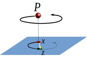
(a) 3D motion

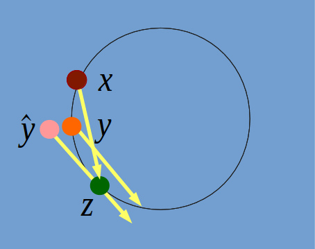
(b) Image plane projection:
Blur kernels from linear displacements

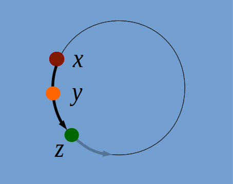
(c) Image plane projection:
Blur kernels from homographies

Figure 10: Inducing blur matrices: LABEL:sub@fig:pptKernel:3D Assume that 3D point $P$ moves with a constant rigid body motion in 3D, e. g. with a yaw motion. The projection of this motion to the image plane (blue) is a circular trajectory. The corresponding 2D ground truth displacement (yellow), however, is a vector in the image plane that connects start and end point of the motion during a time interval. LABEL:sub@fig:pptKernel:2D Using optical flow, the blur kernel at a location $z$ is approximated by identifying all pixels that, according to their spatially-variant displacement, pass through $z$ during the time interval. The image content at point $x$ is correctly identified as passing through $z$. The image content at point $y$ is not identified correctly as its 2D displacement passes $z$ at a distance. Instead, the image content at point $\hat{y}$ is erroneously identified as passing through $z$, even though $\hat{y}$ has a different distance to the rotation center than $z$. This results in the distorted kernels shown in Fig. 3b. LABEL:sub@fig:pptKernel:hom Assuming 3D points in the vicinity of $P$ to form a plane, we employ 3D homographies to generate blur kernels. The blur kernel at location $z$ is thus formed by the image points whose trajectory, according to the homography, passes through $z$ during the time interval. Consequently, $y$ is correctly identified as passing through $z$, leading to the kernels shaped as circular arcs shown in Fig. 3a

G Over-segmentation of Non-Planar Scenes

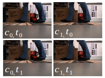
(a) Input

(b) Over-segmentation

(c) 2D projection of scene flow

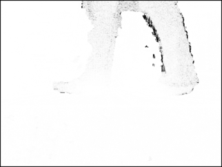
(d) Final occlusion weights

Figure 11: Stereo video deblurring: For two consecutive frames of stereo video LABEL:sub@fig:sceneFlow2:input we use the scene flow approach of Vogel et al. [6] to compute an over-segmentation into planar patches with constant 3D rigid body motion LABEL:sub@fig:sceneFlow2:overseg. For the real scenes shown, we obtain $1000-1500$ segments per frame-pair. For adjacent planes, the projection onto the image plane results in smoothly varying optical flow LABEL:sub@fig:sceneFlow2:OF. At object boundaries, discontinuities in the flow coincide with segment boundaries. We use occlusion information from the scene flow to initialize object boundary weights. The weights are refined iteratively to downweight pixels that do not satisfy our image formation model LABEL:sub@fig:sceneFlow2:weights

To enable the use of homographies, we assume that the scene consist of planes. For objects of arbitrary shape, we approximate their geometry with a collection of planar patches. Figure 10b shows the piecewise planar approximations for real scenes. In all our experiments we obtained approximations with $1000-1500$ planar patches of different 3D motions for images of size $640\times 480$ pixels.

H Deblurring Planar Patches

In the main paper we show that homography-based deblurring improves the PSNR for a planar texture undergoing 3 different 3D motions. Here we provide additional results using other textures and types of motions to show that the improvement generalizes. Fig. 3 shows the different planar textures undergoing various 3D motions. The difference images (Figs. 11c and 11e) show that in all cases homography-based deblurring removes subtle errors that optical flow-based kernel approximation accumulates all over the texture. Additionally, some localized error of the initial optical flow estimation is also corrected in our stereo video deblurring (e. g. rows 2, 4, 6). We average the performance for each motion across the different textures and summarize the results in Table 4. We observe that scene flow-based stereo video deblurring outperforms all other methods for all motions. In particular, averaged over all textures, it outperforms kernels from 2D ground truth flow also in the case of the 2D ‘upward’ motion. This is due to the fact that homographies are invertible and do not suffer from the same rasterization artifacts as kernel generation through forward warping with optical flow.

Table 4: Deblurring planar textures without motion discontinuities: We report the peak signal-to-noise ratio (PSNR) of the deblurred reference frame, the average endpoint error (AEP) of the optical flow, and the average disparity error (ADE). All values are averaged over 8 different planar textures. For all motions the use of scene flow increases deblurring accuracy compared to using 2D displacements. Best results (bold) are obtained with homography based deblurring

blur kernel	ground truth	initial optical		2D projection		3D
source	2D displacement	flow [46]		of scene flow		homographies
	PSNR	AEP	PSNR	AEP	PSNR	ADE	PSNR
forward + roll	32.32	0.10	32.64	0.10	32.73	0.20	33.57
forward	34.22	0.10	34.60	0.09	34.83	0.22	35.40
upward	26.94	0.37	26.75	0.17	26.88	0.97	26.95
forward + yaw	29.40	0.15	29.43	0.14	29.43	0.40	30.56
yaw	26.86	3.01	25.37	0.47	26.81	0.28	27.32
lateral + pitch	28.26	0.15	28.13	0.20	28.23	0.02	29.18

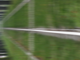
(a) Input

(b) Using kernels from
initial optical flow

(c) Difference (b) to
reference image

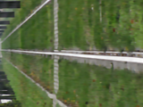
(d) Using kernels
from homographies

(e) Difference (d) to
reference image

Figure 12: Deblurring various planar textures: For a planar texture blurred with 3D rigid body motion LABEL:sub@fig:planar2:input, deblurring with initial optical flow estimates LABEL:sub@fig:planar2:GT yields differences LABEL:sub@fig:planar2:GTdiff to the sharp reference image due to wrongly estimated flow and due to approximated kernels. These errors can be reduced by deblurring with our image formation model that uses scene flow to compute more robust motion and more accurate blur matrices LABEL:sub@fig:planar2:3SF, LABEL:sub@fig:planar2:3SFdiff

I Evaluation of the Structural Similarity Index

In the main paper we report the peak-signal-to-noise-ratio (PSNR) between sharp reference images and deblurred images. However, to be e. g. consistent with human perception, also other evaluation measures for deblurred images are used. In Table 5 we evaluate the Structural Similarity (SSIM) index [47] between deblurred images and sharp reference images. The evaluation confirms the favorable results of visual inspection and the evaluation with the PSNR: In all but the ’apples’ scene, the use of 3D homographies increases SSIM in comparison to using any form of 2D displacement for blur kernel generation. By suppressing locations with invalid image formation model, the influence of motion boundaries and erroneous scene flow computation can be compensated for and our full algorithm obtains consistently better results than deblurring based on 2D displacements.

Table 5: Deblurring with motion discontinuities: While Tab. 3 evaluates PSNR as error measure, here the Structural Similarity (SSIM) index [47] of deblurred synthetic scenes with motion discontinuities (top) and real scenes with the camera moving on a motorized rail (bottom) is evaluated. Also for this evaluation measure, our homography-based stereo video deblurring with motion boundary weighting (full) clearly outperforms monocular video deblurring with optical-flow induced blur kernels

	initial optical	2D projection	3D	ours
	flow [46]	of scene flow	homographies	(full)	Kim and Lee [7]
apples	0.881	0.939	0.928	0.950	0.928
bunny	0.770	0.797	0.826	0.834	0.720
chair	0.817	0.853	0.876	0.905	0.835
squares	0.709	0.776	0.810	0.869	0.796
triplane	0.818	0.830	0.866	0.869	0.693
bottles	0.955	0.953	0.972	0.972	0.942
office	0.958	0.956	0.968	0.968	0.935
planar	0.961	0.961	0.975	0.976	0.945
toys	0.953	0.954	0.967	0.967	0.931

References

- [1] Longuet-Higgins, H.C.: A computer algorithm for reconstructing a scene from two projections. Nature 293 (September 1981) 133–135
- [2] Shotton, J., Girshick, R., Fitzgibbon, A., Sharp, T., Cook, M., Finocchio, M., Moore, R., Kohli, P., Criminisi, A., Kipman, A., Blake, A.: Efficient human pose estimation from single depth images. IEEE T. Pattern Anal. Mach. Intell. 35(12) (December 2013) 2821–2840
- [3] Franke, U., Joos, A.: Real-time stereo vision for urban traffic scene understanding. In: Intelligent Vehicles Symposium. (2000) 273–278
- [4] Geiger, A., Lenz, P., Urtasun, R.: Are we ready for autonomous driving? The KITTI vision benchmark suite. In: CVPR 2012. 3354–3361
- [5] Menze, M., Geiger, A.: Object scene flow for autonomous vehicles. In: CVPR 2015. 3061–3070
- [6] Vogel, C., Schindler, K., Roth, S.: 3D scene flow estimation with a piecewise rigid scene model. Int. J. Comput. Vision 115(1) (October 2015) 1–28
- [7] Hyun Kim, T., Mu Lee, K.: Generalized video deblurring for dynamic scenes. In: CVPR 2015. 5426–5434
- [8] Li, Y., Kang, S.B., Joshi, N., Seitz, S.M., Huttenlocher, D.P.: Generating sharp panoramas from motion-blurred videos. In: CVPR 2010. 2424–2431
- [9] Yahyanejad, S., Strom, J.: Removing motion blur from barcode images. In: CVPR 2010. 41–46
- [10] Fergus, R., Singh, B., Hertzmann, A., Roweis, S.T., Freeman, W.T.: Removing camera shake from a single photograph. SIGGRAPH 2006 787–794
- [11] Cho, S., Lee, S.: Fast motion deblurring. ACM T. Graphics 28(5) (December 2009) 145:1–145:8
- [12] Whyte, O., Sivic, J., Zisserman, A., Ponce, J.: Non-uniform deblurring for shaken images. In: CVPR 2010. 491–498
- [13] Krishnan, D., Tay, T., Fergus, R.: Blind deconvolution using a normalized sparsity measure. In: CVPR 2011. 233–240
- [14] Xu, L., Zheng, S., Jia, J.: Unnatural sparse representation for natural image deblurring. In: CVPR 2013. 1107–1114
- [15] Michaeli, T., Irani, M.: Blind deblurring using internal patch recurrence. In: ECCV 2014. Volume 1. 171–184
- [16] Schelten, K., Roth, S.: Localized image blur removal through non-parametric kernel estimation. In: ICPR 2014. 702–707
- [17] Couzinié-Devy, F., Sun, J., Alahari, K., Ponce, J.: Learning to estimate and remove non-uniform image blur. In: CVPR 2013. 1075–1082
- [18] Wulff, J., Black, M.J.: Modeling blurred video with layers. In: ECCV 2014. Volume 1. 236–252
- [19] Tai, Y.W., Tan, P., Brown, M.S.: Richardson-lucy deblurring for scenes under a projective motion path. IEEE T. Pattern Anal. Mach. Intell. 33(8) (2011) 1603–1618
- [20] Gupta, A., Joshi, N., Zitnick, C.L., Cohen, M., Curless, B.: Single image deblurring using motion density functions. In: ECCV 2010. Volume 1. 171–184
- [21] Rajagopalan, A., Chellappa, R.: Motion Deblurring: Algorithms and Systems. Cambridge University Press (2014)
- [22] Levin, A.: Blind motion deblurring using image statistics. In: NIPS*2006. 841–848
- [23] Chakrabarti, A., Zickler, T., Freeman, W.T.: Analyzing spatially-varying blur. In: CVPR 2010. 2512–2519
- [24] Kim, T.H., Ahn, B., Lee, K.M.: Dynamic scene deblurring. In: ICCV 2013. 3160–3167
- [25] Sun, J., Cao, W., Xu, Z., Ponce, J.: Learning a convolutional neural network for non-uniform motion blur removal. In: CVPR 2015. 769–777
- [26] Kim, T.H., Lee, K.M.: Segmentation-free dynamic scene deblurring. In: CVPR 2014. 2766–2773
- [27] Xu, L., Jia, J.: Depth-aware motion deblurring. In: ICCP. (2012) 1–8
- [28] Lee, H., Lee, K.: Dense 3d reconstruction from severely blurred images using a single moving camera. In: CVPR 2013. 273–280
- [29] Arun, M., Rajagopalan, A., Seetharaman, G.: Multi-shot deblurring for 3d scenes. In: CVPR 2015. 19–27
- [30] Hu, Z., Xu, L., Yang, M.H.: Joint depth estimation and camera shake removal from single blurry image. In: CVPR 2014. 2893–2900
- [31] Cho, S., Matsushita, Y., Lee, S.: Removing non-uniform motion blur from images. In: ICCV 2007. 1–8
- [32] He, X., Luo, T., Yuk, S., Chow, K., Wong, K.Y., Chung, R.: Motion estimation method for blurred videos and application of deblurring with spatially varying blur kernels. In: ICCIT. (2010) 355–359
- [33] Deng, X., Shen, Y., Song, M., Tao, D., Bu, J., Chen, C.: Video-based non-uniform object motion blur estimation and deblurring. Neurocomputing 86 (2012) 170–178
- [34] Yamaguchi, T., Fukuda, H., Furukawa, R., Kawasaki, H., Sturm, P.: Video deblurring and super-resolution technique for multiple moving objects. In: Computer Vision–ACCV 2010. Springer (2010) 127–140
- [35] Vedula, S., Baker, S., Rander, P., Collins, R., Kanade, T.: Three-dimensional scene flow. In: ICCV 1999. Volume 2. 722–729
- [36] Quiroga, J., Devernay, F., Crowley, J.: Local/global scene flow estimation. In: ICIP. (2013) 3850–3854
- [37] Wedel, A., Cremers, D.: Stereo scene flow for 3D motion analysis. Springer Science & Business Media (2011)
- [38] Tai, Y.W., Du, H., Brown, M.S., Lin, S.: Correction of spatially varying image and video motion blur using a hybrid camera. IEEE T. Pattern Anal. Mach. Intell. 32(6) (2010) 1012–1028
- [39] Chen, J., Yuan, L., Tang, C.K., Quan, L.: Robust dual motion deblurring. In: CVPR 2008. 1–8
- [40] Cho, S., Wang, J., Lee, S.: Video deblurring for hand-held cameras using patch-based synthesis. ACM T. Graphics 31(4) (2012) 64:1–64:9
- [41] Joshi, N., Kang, S.B., Zitnick, C.L., Szeliski, R.: Image deblurring using inertial measurement sensors. ACM T. Graphics 29(4) (2010) 30:1–30:9
- [42] Mei, C., Reid, I.: Modeling and generating complex motion blur for real-time tracking. In: CVPR 2008. 1–8
- [43] Murray, R.M., Li, Z., Sastry, S.S.: A mathematical introduction to robotic manipulation. CRC press (1994)
- [44] Portz, T., Zhang, L., Jiang, H.: Optical flow in the presence of spatially-varying motion blur. In: CVPR 2012. 1752–1759
- [45] Levin, A., Weiss, Y.: User assisted separation of reflections from a single image using a sparsity prior. IEEE T. Pattern Anal. Mach. Intell. 29(9) (September 2007) 1647–1654
- [46] Vogel, C., Schindler, K., Roth, S.: An evaluation of data costs for optical flow. In: Pattern Recognition (GCPR) 2013. 343–353
- [47] Wang, Z., Bovik, A.C., Sheikh, H.R., Simoncelli, E.P.: Image quality assessment: From error visibility to structural similarity. IEEE T. Image Process. 13(4) (2004) 600–612