High-order implicit Galerkin-Legendre spectral method for the two-dimensional Schrödinger equation

Abstract

In this paper, we propose Galerkin-Legendre spectral method with implicit Runge-Kutta method for solving the unsteady two-dimensional Schrödinger equation with nonhomogeneous Dirichlet boundary conditions and initial condition. We apply a Galerkin-Legendre spectral method for discretizing spatial derivatives, and then employ the implicit Runge-Kutta method for the time integration of the resulting linear first-order system of ordinary differential equations in complex domain. We derive the spectral rate of convergence for the proposed method in the $L^{2}$-norm for the semidiscrete formulation. Numerical experiments show our formulation have high-order accurate.

1 Introduction

In this paper, we introduce Galerkin-Legendre spectral method for the two-dimensional Schrödinger equation

$$-{\rm i}\frac{\partial u}{\partial t}=\Delta u+\psi(x,y)u,\ (x,y,t)\in(c,d)\times(c,d)\times(t_{0},T),$$ (1.1a)

with the initial condition

$$u(x,y,t_{0})=\varphi(x,y),\ (x,y)\in\Omega=(c,d)\times(c,d),$$ (1.1b)

and the Dirichlet boundary conditions

$$\begin{split}&u(x,c,t)=g_{1}(x,t),\ u(x,d,t)=g_{2}(x,t),\;(x,t)\in(c,d)\times(t_{0},T),\\ &u(c,y,t)=g_{3}(y,t),\ u(d,y,t)=g_{4}(y,t),\;(y,t)\in(c,d)\times(t_{0},T),\\ \end{split}$$ (1.1c)

where $u$ is a complex-valued function, $\psi$ is a smooth known real function, $\varphi$ and $\{g_{j}\}_{j=1}^{4}$ are smooth known complex functions, and ${\rm i}=\sqrt{-1}$.

The Schrödinger equation is a famous equation used widely in many fields of physics [1, 2, 3], such as quantum mechanics, quantum dynamics calculations, optics, underwater acoustics, plasma physics and electromagnetic wave propagation.

Over the past few years, several numerical schemes have been developed for solving problem (1.1). For instance, In [4] Subasi used a standard finite difference method in space for solving the problem (1.1). A Crank-Nicolson method discretization for the time of the problem (1.1) was considered in in [5]. An implicit semi-discrete higher order compact (HOC) scheme was considered for computing the solution of the problem (1.1) in [6]. Dehghana and Shokriin [7] proposed a numerical scheme to solve the problem (1.1) by collocation and radial basis functions in space. A meshless local boundary integral equation (LBIE) method to solve the problem (1.1) was given in [8]. In [1] Mohebbi and Dehghan presented a high order method for the problem (1.1) by the compact finite difference in space and boundary value method in time.In [9] Tian and Yu proposed a HOC-ADI method to solve the problem (1.1), which has fourth-order accuracy in space and second-order accuracy in time. Gao and Xie [10] proposed a numerical scheme to solve the problem (1.1) by the ADI compact finite difference scheme. For the spatial discretisation of the problem (1.1) by the Chebyshev spectral collocation method considered in [2]. In [3] Dehghan and Emami-Naeini presented Sinc-collocation and Sinc-Galerkin methods to solve the problem (1.1).

In this paper, we propose a numerical scheme for solving (1.1). We apply Galerkin-Legendre spectral method [11, 12, 13] for discretizing spatial derivatives, then using the implicit Runge-Kutta method for time derivatives, which is high-order accurate both in space and time.

The contents of the article is as follows. In Section 2, we introduce the implicit Runge-Kutta method for the system of ordinary differential equations in the complex domain. In Section 3, we describe the Galerkin-Legendre spectral method for the two-dimensional Schrödinger equation in space. In Section 4, we derive a priori error estimates in the $L^{2}$-norm for the semidiscrete formulation. The analysis relies on an idea suggested by Lions et al. [14] and Thomée [15]. In Section 5, we report the numerical experiments of solving two-dimensional Schrödinger equation with the new method developed in this paper, and compare the numerical results with analytical solutions and with other method in the literature [1]. We end this article with some concluding remarks in Section 6.

2 Implicit Runge-Kutta method

In this section we modifed the implicit Runge-Kutta (IRK) method to solve first-order linear complex ordinary differential equations. We first give the definition of Kronecker product of matrices.

Definition 2.1 (see, e.g., [16]).

Let $\boldsymbol{A}=(a_{ij})_{m\times n}$ and $\boldsymbol{B}$ be arbitrary matrices, then the matrix

$$\boldsymbol{A}\otimes\boldsymbol{B}=\left(\begin{array}[]{cccc}a_{11}\boldsymbol{B}&a_{12}\boldsymbol{B}&\ldots&a_{1n}\boldsymbol{B}\\ a_{21}\boldsymbol{B}&a_{22}\boldsymbol{B}&\ldots&a_{2n}\boldsymbol{B}\\ \vdots&\vdots&\ddots&\vdots\\ a_{m1}\boldsymbol{B}&a_{m2}\boldsymbol{B}&\ldots&a_{mn}\boldsymbol{B}\\ \end{array}\right),$$

is called the Kronecker product of $\boldsymbol{A}$ and $\boldsymbol{B}$.

Definition 2.2 (see, e.g., [16]).

Let $\boldsymbol{A}=(a_{ij})_{m\times n}$ be any given matrix, then ${\rm vec}(\boldsymbol{A})$ is defined to be a column vector of size $m\times n$ made of the row of

$${\rm vec}(\boldsymbol{A})=(a_{11},a_{12},\ldots,a_{1n},a_{21},a_{22},\ldots,a_{m1},\ldots,a_{mn})^{T}.$$

Lemma 2.1 (see, e.g., [16]).

Let $\boldsymbol{A}=(a_{ij})_{m\times n}$, $\boldsymbol{B}=(b_{ij})_{n\times p}$, and $\boldsymbol{C}=(c_{ij})_{p\times q}$ be three given matrices. Then

$${\rm vec}(\boldsymbol{A}\boldsymbol{B}\boldsymbol{C})=(\boldsymbol{A}\otimes\boldsymbol{C}^{T}){\rm vec}(\boldsymbol{B}).$$

Lemma 2.2 (see, e.g., [16]).

Let $\boldsymbol{A}=(a_{ij})_{m\times 1}$, $\boldsymbol{B}=(b_{ij})_{n\times 1}$. Then

$${\rm vec}(\boldsymbol{A}\boldsymbol{B}^{T})=\boldsymbol{A}\otimes\boldsymbol{B}.$$

We consider the following first-order initial value problem is given by

$$\begin{cases}y^{\prime}=f(t,y(t)),\;\;t_{0}<t\leq T,\\ y(t_{0})=y_{0}.\end{cases}$$ (2.1)

A $s$-stage formula of implicit Runge-Kutta method for approximating (2.1) can be written as

$$\begin{cases}y_{n+1}={y_{n}}+h\sum\limits_{l=1}^{s}{{b_{l}}}f\left({{t_{n}}+{c_{l}}h,{k_{l}}}\right),\\ {k_{l}}={y_{n}}+h\sum\limits_{j=1}^{s}{{a_{lj}}}f\left({{t_{n}}+{c_{j}}h,{k_{j}}}\right),\quad l=1,2,\ldots,s,\end{cases}$$ (2.2)

where $h=(T-t_{0})/(N_{t}-1)$ is the integration step, $\{k_{l}\}_{l=1}^{s}$ are the internal stages and $t_{n}=t_{0}+hn$. If $a_{lj}=0\,(l>j)$ the method is called diagonally implicit Runge-Kutta (DIRK) method. Then the (2.2) can be written the following form

$$\begin{cases}\boldsymbol{K}={\boldsymbol{1}}_{s}y_{n}+h\boldsymbol{A}\boldsymbol{F}(\boldsymbol{K}),\\ y_{n+1}={y_{n}}+h\boldsymbol{B}^{T}\boldsymbol{F}(\boldsymbol{K}),\end{cases}$$ (2.3)

where $A=(a_{lj})_{l,j=1,\ldots,s},$ $\boldsymbol{B}=[b_{1},b_{2},\cdots,b_{s}]^{T}$, $\boldsymbol{K}=[k_{1},k_{2},\cdots,k_{s}]^{T}$, ${\boldsymbol{1}}_{s}=[\underbrace{1,1,\cdots,1}_{s}]^{T}$, and

$$\boldsymbol{F}(\boldsymbol{K})=[f(t_{n}+c_{1}h,k_{1}),f(t_{n}+c_{2}h,k_{2}),\cdots,f(t_{n}+c_{s}h,k_{s})]^{T}.$$

If we consider the system of linear ordinary differential equations

$$\begin{cases}-{\rm i}\boldsymbol{M}_{1}\boldsymbol{y}^{\prime}+\boldsymbol{M}_{2}\boldsymbol{y}-\boldsymbol{f}(t)=0,\ \ t_{0}<t\leq T,\\ \boldsymbol{y}(t_{0})=\boldsymbol{y}_{0},\end{cases}$$ (2.4)

where $\boldsymbol{M}_{1},\boldsymbol{M}_{2}\in\mathbb{R}_{m\times m}$, and

$$\boldsymbol{y}(t)=[y_{1}(t),y_{2}(t),\cdots,y_{m}(t)]^{T},\;\;\boldsymbol{f}(t)=[f_{1}(t),f_{2}(t),\cdots,f_{m}(t)]^{T}.$$

Using s-stage formula of Runge-Kutta method (2.3) for approximating (2.4) can be written as

$$\begin{cases}-{\rm i}\boldsymbol{K}\boldsymbol{M}_{1}^{T}=-{\rm i}{\boldsymbol{1}}_{s}\boldsymbol{y}_{n}^{T}\boldsymbol{M}_{1}^{T}+h\boldsymbol{A}(-\boldsymbol{K}\boldsymbol{M}_{2}^{T}+\boldsymbol{F}),\\ -{\rm i}\boldsymbol{y}_{n+1}^{T}\boldsymbol{M}_{1}^{T}=-{\rm i}{\boldsymbol{y}_{n}^{T}}\boldsymbol{M}_{1}^{T}+h\boldsymbol{B}^{T}(-\boldsymbol{K}\boldsymbol{M}_{2}^{T}+\boldsymbol{F}),\end{cases}$$ (2.5)

where

$$\begin{split}&\boldsymbol{K}=[\boldsymbol{k}_{1}^{T};\boldsymbol{k}_{2}^{T};\cdots;\boldsymbol{k}_{s}^{T}],\;\;\boldsymbol{F}=[\boldsymbol{f}(t_{n}+c_{1}h)^{T};\boldsymbol{f}(t_{n}+c_{2}h)^{T};\cdots;\boldsymbol{f}(t_{n}+c_{s}h)^{T}].\end{split}$$

By using Lemma 2.1 and 2.2, we have

$$(-{\rm i}\boldsymbol{I}_{s}\otimes\boldsymbol{M}_{1}+h\boldsymbol{A}\otimes\boldsymbol{M}_{2}){\rm vec}(\boldsymbol{K})=-{\rm i}{\boldsymbol{1}}_{s}\otimes(\boldsymbol{M}_{1}{\boldsymbol{y}}_{n})+h\boldsymbol{A}\otimes\boldsymbol{I}_{m}{\rm vec}(\boldsymbol{F}),$$ (2.6)

where $\boldsymbol{I}_{s}$ is the $s\times s$ unitary matrix. Thus we can obtain ${\rm vec}(\boldsymbol{K})$ from (2.6) with GMRES iteration (see, e.g., [11, PP. 55–58]).

We write the Runge-Kutta scheme in a tabular format known as the Butchers table, in Table 2.1, we choose a 3-stage IRK method (cf. [17]).

Table 2.1: Left: Butchers table. Right: 3-stage IRK method

$c_{1}$	$a_{11}$	$\cdots$	$a_{1s}$
$\vdots$	$\vdots$	$\ddots$	$\vdots$
$c_{s}$	$a_{11}$	$\cdots$	$a_{ss}$
	$b_{1}$	$\cdots$	$b_{s}$

$\frac{1}{2}-\frac{\sqrt{15}}{10}$	$\frac{5}{36}$	$\frac{2}{9}-\frac{\sqrt{15}}{15}$	$\frac{5}{36}-\frac{\sqrt{15}}{30}$
$\frac{1}{2}$	$\frac{5}{36}+\frac{\sqrt{15}}{24}$	$\frac{2}{9}$	$\frac{5}{36}-\frac{\sqrt{15}}{24}$
$\frac{1}{2}+\frac{\sqrt{15}}{10}$	$\frac{5}{36}+\frac{\sqrt{15}}{30}$	$\frac{2}{9}+\frac{\sqrt{15}}{15}$	$\frac{5}{36}$
	$\frac{5}{18}$	$\frac{4}{9}$	$\frac{5}{18}$

3 Discretize two-dimensional Schrödinger equation in space by Galerkin-Legendre spectral method

In this section, we will present the Galerkin-Legendre spectral method to solve the unsteady two-dimensional Schrödinger equation for the space with the nonhomogeneous Dirichlet boundary conditions and initial condition. Firstly, we make the variable transformations

$$x=c+\frac{\tilde{x}+1}{2}(d-c),\ y=c+\frac{\tilde{y}+1}{2}(d-c),\ \gamma=\Big{(}\frac{2}{d-c}\Big{)}^{2},$$

$$\tilde{u}(\tilde{x},\tilde{y},t)=u\big{(}c+\frac{\tilde{x}+1}{2}(d-c),c+\frac{\tilde{y}+1}{2}(d-c),t\big{)},$$

$$\tilde{\psi}(\tilde{x},\tilde{y})=\psi\big{(}c+\frac{\tilde{x}+1}{2}(d-c),c+\frac{\tilde{y}+1}{2}(d-c)\big{)},$$

$$\tilde{\varphi}(\tilde{x},\tilde{y})=\varphi\big{(}c+\frac{\tilde{x}+1}{2}(d-c),c+\frac{\tilde{y}+1}{2}(d-c)\big{)},$$

$$\tilde{g}_{1}(\tilde{y},t)=g_{1}\big{(}c+\frac{\tilde{y}+1}{2}(d-c),t\big{)},\ \tilde{g}_{2}(\tilde{y},t)=g_{2}\big{(}c+\frac{\tilde{y}+1}{2}(d-c),t\big{)},$$

$$\tilde{g}_{3}(\tilde{x},t)=g_{3}\big{(}c+\frac{\tilde{x}+1}{2}(d-c),t\big{)},\ \tilde{g}_{4}(\tilde{x},t)=g_{4}\big{(}c+\frac{\tilde{x}+1}{2}(d-c),t\big{)}.$$

Then $\Omega$ is changed to the square $\widetilde{\Omega}=(-1,1)\times(-1,1)$, and the (1.1) can be rewritten as

$$-{\rm i}\frac{\partial\tilde{u}}{\partial t}=\gamma\Delta\tilde{u}+\tilde{\psi}(\tilde{x},\tilde{y})\tilde{u},\;\;(\tilde{x},\tilde{y},t)\in\widetilde{\Omega}\times(t_{0},T),$$ (3.1a)

with the initial condition

$$\tilde{u}(\tilde{x},\tilde{y},t_{0})=\tilde{\varphi}(\tilde{x},\tilde{y}),\ {\rm on}\;\;\widetilde{\Omega},$$ (3.1b)

and the Dirichlet boundary conditions

$$\begin{split}&\tilde{u}(-1,y,t)=\tilde{g}_{1}(y,t),\ \tilde{u}(1,\tilde{y},t)=\tilde{g}_{2}(\tilde{y},t),\ {\rm on}\ J=(t_{0},T),\\ &\tilde{u}(\tilde{x},-1,t)=\tilde{g}_{3}(\tilde{x},t),\ \tilde{u}(\tilde{x},1,t)=\tilde{g}_{4}(\tilde{x},t),\ {\rm on}\ J=(t_{0},T).\end{split}$$ (3.1c)

Now we recall the boundary conditions homogeneous process (see, e.g., [13]). Setting

$$\tilde{u}_{1}(\tilde{x},\tilde{y},t)=\frac{\tilde{g}_{4}(\tilde{x},t)-\tilde{g}_{3}(\tilde{x},t)}{2}\tilde{y}+\frac{\tilde{g}_{4}(\tilde{x},t)+\tilde{g}_{3}(\tilde{x},t)}{2},$$

$$\hat{g}_{1}(\tilde{y},t)=\tilde{g}_{1}(\tilde{y},t)-\tilde{u}_{1}(-1,\tilde{y},t),\ \hat{g}_{2}(\tilde{y},t)=\tilde{g}_{2}(\tilde{y},t)-\tilde{u}_{1}(1,\tilde{y},t),$$

$$\tilde{u}_{2}(\tilde{x},\tilde{y},t)=\frac{\hat{g}_{2}(\tilde{y},t)-\hat{g}_{1}(\tilde{y},t)}{2}\tilde{x}+\frac{\hat{g}_{2}(\tilde{y},t)+\hat{g}_{1}(\tilde{y},t)}{2},$$

$$\hat{u}=\tilde{u}-\tilde{u}_{1}-\tilde{u}_{2},$$

$$\tilde{f}(\tilde{x},\tilde{y},t)={\rm i}\Big{(}\frac{\partial\tilde{u}_{1}}{\partial t}+\frac{\partial\tilde{u}_{2}}{\partial t}\Big{)}+\gamma(\Delta\tilde{u}_{1}+\Delta\tilde{u}_{2})+\tilde{\psi}(\tilde{u}_{1}+\tilde{u}_{2}),$$

$$\hat{\varphi}(\tilde{x},\tilde{y})=\tilde{\varphi}(\tilde{x},\tilde{y})-\tilde{u}_{1}(\tilde{x},\tilde{y},t_{0})-\tilde{u}_{2}(\tilde{x},\tilde{y},t_{0}),$$

then the (3.1) can be rewritten as

$$-{\rm i}\frac{\partial\hat{u}}{\partial t}=\gamma\Delta\hat{u}+\tilde{\psi}(\tilde{x},\tilde{y})\hat{u}+\tilde{f}(\tilde{x},\tilde{y},t),\ (\tilde{x},\tilde{y},t)\in(-1,1)\times(-1,1)\times(t_{0},T),$$ (3.2a)

with the initial condition and homogeneous boundary value conditions

$$\begin{split}\hat{u}(\tilde{x},\tilde{y},t_{0})=&\hat{\varphi}(\tilde{x},\tilde{y}),\,{\rm on}\;\widetilde{\Omega},\\ \hat{u}(\tilde{x},-1,t)=\hat{u}(\tilde{x},1,t)=&\hat{u}(-1,\tilde{y},t)=\hat{u}(1,\tilde{y},t)=0,\,{\rm on}\;J=(t_{0},T).\end{split}$$ (3.2b)

We shall now discretize the equation (3.2) by using the Galerkin-Legendre spectral method in space. Let us denote $L_{n}(\tilde{x})$ the $n$th degree Legendre polynomial (see, e.g., [11, PP. 18 and 19]) and

$$P_{N}=\textup{span}\{L_{0}(\tilde{x}),L_{1}(\tilde{x}),\cdots,L_{N}(\tilde{x})\},\ V_{N}=\{v\in P_{N}:v(\pm 1)=0\}.$$

Then the semi-discrete Legendre-Galerkin method for (3.2) is: find $\hat{u}_{N}:\bar{J}\rightarrow V_{N}^{2}$ such that

$$\left\{\begin{array}[]{ll}-{\rm i}(\partial{{}_{t}}\hat{u}_{N},v)+\gamma(\nabla\hat{u}_{N},\nabla v)-(\tilde{\psi}(\tilde{x},\tilde{y})\hat{u}_{N},v)-(\hat{f}(\tilde{x},\tilde{y},t),v)=0,\quad\forall\,v\in V_{N}^{2},\\ (\hat{u}_{N}(\tilde{x},\tilde{y},t_{0})-\hat{u}_{0},v)=0,\quad\forall\,v\in V_{N}^{2},\end{array}\right.$$ (3.5)

where $(u,v)=\int_{\widetilde{\Omega}}u\bar{v}d\tilde{x}d\tilde{y}$ is the scalar product in $L^{2}(\widetilde{\Omega})$, the $\bar{v}$ is complex conjugate of $v$.

The following lemma is the key to implement our algorithms.

Lemma 3.1.

([13, Lemma 2.1]) Let us denote

$$\phi_{k}(\tilde{x})=c_{k}(L_{k}(\tilde{x})-L_{k+2}(\tilde{x})),\;\;c_{k}=\frac{1}{\sqrt{4k+6}},$$

$$\tilde{a}_{jk}=\int^{1}_{-1}\phi^{\prime}_{k}(\tilde{x})\phi^{\prime}_{j}(\tilde{x})d\tilde{x},\;\;\tilde{b}_{jk}=\int^{1}_{-1}\phi_{k}(\tilde{x})\phi_{j}(\tilde{x})d\tilde{x},$$

then

$$\tilde{a}_{jk}=\left\{\begin{array}[]{ll}1,&k=j,\\ 0,&k\neq j,\end{array}\right.\quad\tilde{b}_{jk}=\tilde{b}_{kj}=\left\{\begin{array}[]{ll}c_{k}c_{j}(\frac{2}{2j+1}+\frac{2}{2j+5}),&k=j,\\ -c_{k}c_{j}\frac{2}{2k+1},&k=j+2,\\ 0,&otherwise.\end{array}\right.$$

Obviously

$$V_{N}=\textup{span}\{\phi_{0}(\tilde{x}),\phi_{1}(\tilde{x}),\cdots,\phi_{N-2}(\tilde{x})\}.$$

Let us setting

$$\hat{u}_{N}(\tilde{x},\tilde{y},t)=\sum_{k,j=0}^{N-2}\alpha_{kj}(t)\phi_{k}(\tilde{x})\phi_{j}(\tilde{y}),$$ (3.6)

then inserting (3.6) into (3.5) and taking

$$v=\phi_{l}(\tilde{x})\phi_{m}(\tilde{y}),$$

yields

$$-{\rm i}\big{(}\partial{{}_{t}}\hat{u}_{N},\phi_{l}(\tilde{x})\phi_{m}(\tilde{y})\big{)} +\gamma\big{(}\nabla\hat{u}_{N},\nabla(\phi_{l}(\tilde{x})\phi_{m}(\tilde{y}))\big{)}-\big{(}\tilde{\psi}(\tilde{x},\tilde{y})\hat{u}_{N},\phi_{l}(\tilde{x})\phi_{m}(\tilde{y})\big{)}$$ (3.7)

$$-\big{(}\hat{f}(\tilde{x},\tilde{y},t),\phi_{l}(\tilde{x})\phi_{m}(\tilde{y})\big{)}=0,\;\;l,m=0,1,\ldots,N-2.$$

Denote ${\boldsymbol{\alpha}}=(\alpha_{kj})_{k,j=0,1,\ldots,N-2},$ and

$$\begin{split}\widetilde{\boldsymbol{B}}=(\tilde{b}_{kj})_{k,j=0,1,\ldots,N-2},\;\;\hat{f}_{kj}=\big{(}\hat{f}(\tilde{x},\tilde{y},t),\phi_{k}(\tilde{x})\phi_{j}(\tilde{y})\big{)},\;\;\widehat{\boldsymbol{F}}(t)=(\hat{f}_{kj})_{k,j=0,1,\ldots,N-2}.\end{split}$$

The (3.7) is equivalent to the following matrix equation

$$-{\rm i}\widetilde{\boldsymbol{B}}\boldsymbol{\alpha}^{\prime}\widetilde{\boldsymbol{B}}+\gamma(\widetilde{\boldsymbol{B}}\boldsymbol{\alpha}\boldsymbol{I}_{N-1}+\boldsymbol{I}_{N-1}\boldsymbol{\alpha}\widetilde{\boldsymbol{B}})-\boldsymbol{W}_{\boldsymbol{\alpha}}-\widehat{\boldsymbol{F}}(t)=0,$$

where ${\boldsymbol{\alpha}}=(\alpha_{kj})_{k,j=0,1,\ldots,N-2}$ and

$$(\boldsymbol{W}_{\boldsymbol{\alpha}})_{lm}=\sum_{k,j=0}^{N-2}\alpha_{kj}(t)\big{(}\tilde{\psi}(\tilde{x},\tilde{y})\phi_{k}(\tilde{x})\phi_{j}(\tilde{y}),\phi_{l}(\tilde{x})\phi_{m}(\tilde{y})\big{)},\ l,m=0,1,\ldots,N-2.$$

Using Lemma 2.1, we have

$$-{\rm i}\widetilde{\boldsymbol{B}}\otimes\widetilde{\boldsymbol{B}}\,{\rm vec}(\boldsymbol{\alpha}^{\prime})+(\gamma\widetilde{\boldsymbol{B}}\otimes I_{N-1}+\gamma\boldsymbol{I}_{N-1}\otimes\widetilde{\boldsymbol{B}}-\widetilde{\boldsymbol{W}}){\rm vec}(\boldsymbol{\alpha})-{\rm vec}(\widehat{\boldsymbol{F}}(t))=0,$$

where $\widetilde{\boldsymbol{W}}_{(l-1)(N-2)+m,(k-1)(N-2)+j}=\big{(}\tilde{\psi}(\tilde{x},\tilde{y})\phi_{k}(\tilde{x})\phi_{j}(\tilde{y}),\phi_{l}(\tilde{x})\phi_{m}(\tilde{y})\big{)},\ l,m,k,j=0,1,\ldots,N-2.$

Setting

$$\hat{u}_{N}(\tilde{x},\tilde{y},t_{0})=\sum_{k,j=0}^{N-2}\alpha_{kj}(t_{0})\phi_{k}(\tilde{x})\phi_{j}(\tilde{y}),$$

and with

$$\big{(}\hat{u}_{N}(\tilde{x},\tilde{y},t_{0})-\hat{\varphi}(\tilde{x},\tilde{y}),\phi_{l}(\tilde{x})\phi_{m}(\tilde{y})\big{)}=0,\;\;l,m=0,1,\ldots,N-2,$$

we obtian

$$\widetilde{\boldsymbol{B}}\boldsymbol{\alpha}(t_{0})\widetilde{\boldsymbol{B}}=\hat{\boldsymbol{u}}_{0},\;\;(\hat{\boldsymbol{u}}_{0})_{kj}=\big{(}\varphi(\tilde{x},\tilde{y}),\phi_{k}(\tilde{x})\phi_{j}(\tilde{y})\big{)}.$$

Using Lemma 2.1, we have

$$\widetilde{\boldsymbol{B}}\otimes\widetilde{\boldsymbol{B}}\,{\rm vec}(\boldsymbol{\alpha}(t_{0}))={\rm vec}(\hat{\boldsymbol{u}}_{0}).$$

Therefore, (3.5) leads to the following system of linear ordinary differential equations

$$\begin{cases}-{\rm i}\widetilde{\boldsymbol{B}}\otimes\widetilde{\boldsymbol{B}}{\rm vec}(\boldsymbol{\alpha}^{\prime})+(\gamma\widetilde{\boldsymbol{B}}\otimes\boldsymbol{I}_{N-1}+\gamma\boldsymbol{I}_{N-1}\otimes\widetilde{\boldsymbol{B}}-\widetilde{\boldsymbol{W}}){\rm vec}(\boldsymbol{\alpha})\\ \hskip 142.26378pt-{\rm vec}(\widehat{\boldsymbol{F}}(t))=0,\quad t_{0}<t\leq T,\\ {\rm vec}(\boldsymbol{\alpha}(t_{0}))=\big{(}\widetilde{\boldsymbol{B}}\otimes\widetilde{\boldsymbol{B}}\big{)}^{-1}{\rm vec}(\hat{\boldsymbol{u}}_{0}).\end{cases}$$ (3.8)

Hence we can use the 3-stage IRK method for (3.8).

4 A priori error estimate

In this section, we derive optimal a priori error bound for the semidiscrete scheme of the problem (1.1) by using the Galerkin-Legendre spectral method discretization for the space. Recall the spaces

$$\begin{split}L^{2}(\widetilde{\Omega})=\{u:(u,u)&<+\infty\},\;\;H^{m}(\widetilde{\Omega})=\{u:{D}^{k}u\in L^{2}(\widetilde{\Omega}),\ 0\leq|k|\leq m\},\\ H^{m}_{0}(\widetilde{\Omega})=&\{u\in H^{m}(\widetilde{\Omega}):{D}^{k}u(\partial\widetilde{\Omega})=0,\ 0\leq|k|\leq m-1\}.\end{split}$$

The norms in $L^{2}(\widetilde{\Omega})$ and $H^{m}(\widetilde{\Omega})$ denoted by $\|\cdot\|$ and $\|\cdot\|_{m}$, respectively, which are given as

$$\|u\|=(u,u)^{1/2},\quad\|u\|_{m}=\Big{(}\sum_{|k|=0}^{m}\|{D}^{k}u\|^{2}\Big{)}^{1/2}.$$

Furthermore, we shall use $|u|_{m}=\Big{(}\sum\limits_{|k|=m}\|{D}^{k}u\|^{2}\Big{)}^{1/2}$ to denote the semi-norm in $H^{m}(\widetilde{\Omega})$. We now introduce the bochner space $L^{p}(J;X)$ endowed with the norm

$$\|v\|_{L^{p};X}=\begin{cases}(\int_{J}\|v\|_{X}^{p}dt)^{1/p},\,\,&1\leq p<\infty,\\ \textup{ess}\sup_{t\in J}\|v\|_{X},\,\,&p=\infty,\\ \end{cases}$$

where $X=L^{2}(\widetilde{\Omega})$ or $X=H^{m}(\widetilde{\Omega})$.

Let $H^{1}_{0}(\widetilde{\Omega})=H^{1}(\widetilde{\Omega})\bigcap\{v|v(\partial\widetilde{\Omega})=0\}.$ The $L^{2}(\widetilde{\Omega})$ orthogonal projection $\Pi^{0}_{N}:H^{1}_{0}(\widetilde{\Omega})\rightarrow V^{2}_{N}$ is defined by

$$(\Pi^{0}_{N}{u}-{u},v)=0,\quad\forall v\in V_{N}^{2}.$$

The operators $\Pi^{0}_{N}$ have the following approximation properties.

Lemma 4.1.

([18, PP. 309 and 310]) For any positive integer $m\geq 1$, the following estimate holds for any ${u}\in H^{m}(\widetilde{\Omega})\bigcap H^{1}_{0}(\widetilde{\Omega})$

$$N\|{u}-\Pi^{0}_{N}{u}\|+\|\nabla({u}-\Pi^{0}_{N}{u})\|\leq CN^{1-m}\|{u}\|_{m},$$

where $C$ is independent of $N$.

We now split the error as a sum of two terms

$$\hat{u}_{N}-\hat{u}=(\hat{u}_{N}-\mathbb{P}^{0}_{N}\hat{u})+(\mathbb{P}^{0}_{N}\hat{u}-\hat{u})=\theta+\rho,$$ (4.1)

where $\mathbb{P}^{0}_{N}\hat{u}$ is an elliptic projection in $V_{N}^{2}$ of the exact solution $\hat{u}$, which defined by

$$\mathcal{A}(\mathbb{P}^{0}_{N}\hat{u}-\hat{u},v)=0,\quad\forall v\in V_{N}^{2}.$$ (4.2)

We begin with the following auxiliary result.

Lemma 4.2.

([18, P. 309] Assume that $\hat{u}\in L^{\infty}(J,H^{m}(\widetilde{\Omega})\cap H^{1}_{0}(\widetilde{\Omega}))$ and $\mathbb{P}^{0}_{N}$ defined by (4.2). Then

$$N\|\mathbb{P}^{0}_{N}\hat{u}-\hat{u}\|+\|\nabla(\mathbb{P}^{0}_{N}\hat{u}-\hat{u})\|\leq CN^{1-m}\|\hat{u}\|_{m},\ \textup{for}\ \ t\in\bar{J},$$

where $C$ is independent of $N$.

Lemma 4.3.

With $\mathbb{P}^{0}_{N}$ defined by (4.2) and $\rho=\mathbb{P}^{0}_{N}\hat{u}-\hat{u}$. Assume that $\hat{u},\partial{{}_{t}}\hat{u}\in L^{\infty}(J,H^{m}(\widetilde{\Omega})\cap H^{1}_{0}(\widetilde{\Omega}))$. Then

$$\|\rho(t)\|\leq CN^{-m}\|\hat{u}\|_{m},\ \textup{for}\ t\in\bar{J},$$

$$\|\partial{{}_{t}}\rho(t)\|\leq CN^{-m}\|\partial{{}_{t}}\hat{u}\|_{m},\ \textup{for}\ \ t\in\bar{J},$$

where $C$ is independent of $N$.

We are now ready for the $L^{2}$-error estimate for the semidiscrete problem.

Theorem 4.1.

Let $\hat{u}$ and $\hat{u}_{N}$ be the solutions of (3.2) and (3.5), respectively. Assume that $\tilde{\psi}$ is a real function, $\tilde{\psi}\in L^{\infty}(\widetilde{\Omega})$ and $\hat{u},\ \partial{{}_{t}}\hat{u}\in L^{\infty}(J,H^{m}(\widetilde{\Omega})\cap H^{1}_{0}(\widetilde{\Omega}))$. Then, we have

$$\begin{split}&\|\hat{u}_{N}(t)-\hat{u}(t)\|\leq CN^{-m}\big{(}\|\hat{u}\|_{L^{\infty}(J;H^{m}(\widetilde{\Omega}))}+\|\partial{{}_{t}}\hat{u}\|_{L^{\infty}(J;H^{m}(\widetilde{\Omega}))}\big{)},\ \textup{for}\ t\in J,\\ \end{split}$$

where $C$ is independent of $N$.

Proof.

With $\hat{u}_{N}$ and $\hat{u}$ satisfies the following equation

$$-{\rm i}(\partial{{}_{t}}\hat{u}_{N},v)+\gamma\mathcal{A}(\hat{u}_{N},v)-(\tilde{\psi}(\tilde{x},\tilde{y})\hat{u}_{N},v)-(\hat{f}(\tilde{x},\tilde{y},t),v)=0,\quad\forall v\in V_{N}^{2},$$

and

$$-{\rm i}(\partial{{}_{t}}\hat{u},v)+\gamma\mathcal{A}(\hat{u},v)-(\tilde{\psi}(\tilde{x},\tilde{y})\hat{u},v)-(\hat{f}(\tilde{x},\tilde{y},t),v)=0,\quad\forall v\in V_{N}^{2}.$$

Hence with $v=\theta$, we obtain

$$\begin{split}-{\rm i}(\partial{{}_{t}}(\theta+\rho),v)+\gamma\mathcal{A}(\theta+\rho,v)-(\tilde{\psi}(\tilde{x},\tilde{y})(\theta+\rho),v)=0,\quad\forall v\in V_{N}^{2}.\end{split}$$

Taking both sides the imaginary, we obtain

$$\begin{split}\frac{1}{2}\frac{d}{dt}\|\theta\|^{2}=-{\rm Re}(\partial{{}_{t}}\rho,\theta)-{\rm Im}(\tilde{\psi}(\tilde{x},\tilde{y})\rho,\theta),\end{split}$$

such that

$$\frac{1}{2}\frac{d}{dt}\|\theta\|^{2}\leq C(\|\theta\|^{2}+\|\rho\|^{2}+\|\partial{{}_{t}}\rho\|^{2}).$$

After integration, this shows

$$\|\theta(t)\|^{2}\leq C\|\theta(t_{0})\|^{2}+C\int^{t}_{t_{0}}(\|\theta\|^{2}+\|\rho\|^{2}+\|\partial{{}_{s}}\rho\|^{2})ds.$$

By using the Gronwall’s Lemma, we have

$$\|\theta(t)\|^{2}\leq C\|\theta(t_{0})\|^{2}+C\int^{t}_{t_{0}}(\|\rho\|^{2}+\|\partial{{}_{s}}\rho\|^{2})ds.$$

By Lemma 4.3, we have

$$\begin{split}\|\theta(t)\|^{2}\leq&C\|\theta(t_{0})\|^{2}+CN^{-2m}(T-t_{0})\big{(}\|\hat{u}\|_{L^{\infty}(J;H^{m}(\widetilde{\Omega}))}^{2}+\|\partial{{}_{t}}\hat{u}\|_{L^{\infty}(J;H^{m}(\widetilde{\Omega}))}^{2}\big{)}\\ \leq&C_{5}N^{-2m}\big{(}\|\hat{u}\|_{L^{\infty}(J;H^{m}(\widetilde{\Omega}))}^{2}+\|\partial{{}_{t}}\hat{u}\|_{L^{\infty}(J;H^{m}(\widetilde{\Omega}))}^{2}\big{)}.\end{split}$$

Using Lemmas 4.1 and 4.2, we obtain

$$\begin{split}\|\theta(t_{0})\|=&\|\hat{u}_{N}(t_{0})-\mathbb{P}^{0}_{N}\hat{u}(t_{0})\|\leq\|\Pi^{0}_{N}\hat{u}(t_{0})-\hat{u}(t_{0})\|+\|\mathbb{P}^{0}_{N}\hat{u}(t_{0})-\hat{u}(t_{0})\|\\ \leq&CN^{-m}\big{(}\|\hat{u}\|_{L^{\infty}(J;H^{m}(\widetilde{\Omega}))}+\|\partial{{}_{t}}\hat{u}\|_{L^{\infty}(J;H^{m}(\widetilde{\Omega}))}\big{)}.\end{split}$$

Then we have

$$\begin{split}\|\hat{u}_{N}(t)-\hat{u}(t)\|\leq&\|\theta(t)\|+\|\rho(t)\|\leq CN^{-m}\big{(}\|\hat{u}\|_{L^{\infty}(J;H^{m}(\widetilde{\Omega}))}+\|\partial{{}_{t}}\hat{u}\|_{L^{\infty}(J;H^{m}(\widetilde{\Omega}))}\big{)},\end{split}$$

this complete the proof. ∎

5 Numerical results

In this section, we present numerical examples to demonstrate the convergence and accuracy of the new method.

For a given $N$, we denote the discrete $L^{2}$-error by

$$\textup{error}(t)=\Big{(}\sum_{k=0}^{N}\sum_{k=0}^{N}\big{(}v_{N}(x_{k},y_{m},t)-v(x_{k},y_{m},t)\big{)}^{2}\omega_{km}\Big{)}^{\frac{1}{2}}.$$

where $v=\text{Re}(u)$ or $v=\text{Im}(u)$, $x_{k}$, $y_{m}$ are Legendre-Gauss-Lobatto quadrature nodes, $\omega_{km}$ are quadrature weights in $\Omega$ (see, e.g., [12, Theorem 3.29])

5.1 Test Problem 1

We consider problem (1.1) with $c=0$, $d=1$, $t_{0}=0$, $T=1$, $\psi(x,y)=3-2\tanh^{2}(x)-2\tanh^{2}(y)$ and the following initial condition

$$\phi(x,y)=\frac{{\rm i}}{\cosh(x)\cosh(y)},\ x\in(c,d)\times(c,d).$$

The exact solution is given by

$$u(x,y,t)=\frac{{\rm i}\exp({\rm i}t)}{\cosh(x)\cosh(y)}.$$ (5.1)

The boundary conditions can be obtained easily from (5.1).

This test problem is given in [1]. Figure 1 shows the surface plot of absolute error for Test Problem 1 with $N=18$ and $h=1/20$ at $T=1$. Figure 2 shows the surface plot of absolute error for Test Problem 1 by using the method of [1] with $N_{x}=N_{y}=\frac{d-c}{\Delta x}=\frac{d-c}{\Delta y}=20$ and $\Delta t=1/20$. Comparing Figure 1 with Figure 2, we can see that our method is more accurate than the algorithm of [1]. Figure 3 shows the convergence rates for Test problem 1 with $h=1/50$ at $T=1$. The curves show exponential rates of convergence in space.

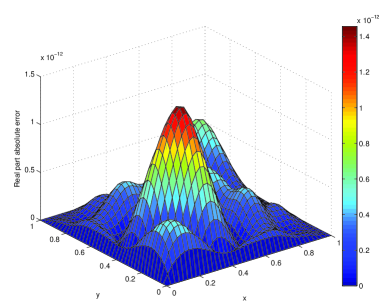
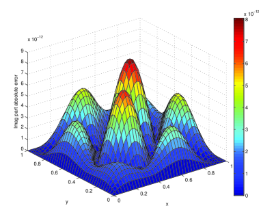
Figure 1: Surface plot of absolute error obtained for Test problem 1 in time with $N=18$ and $h=1/20$ (left panel for real part and right panel for imaginary part).

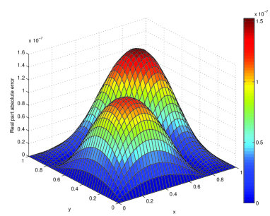
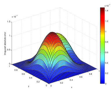
Figure 2: Surface plot of absolute error obtained for Test problem 1 by using the method of [1] with $N_{x}=N_{y}=20$ and $\triangle t=1/20$ (left panel for real part and right panel for imaginary part).

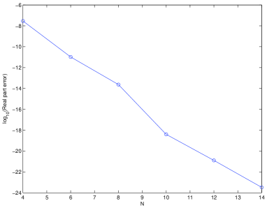
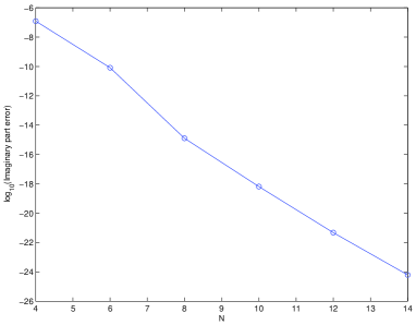
Figure 3: Exponential convergence in $N$ for Test problem 1 with $h=1/50$ (left panel for real part and right panel for imaginary part).

5.2 Test Problem 2

We consider problem (1.1) with $c=-2.5$, $d=2.5$, $t_{0}=0$, $T=1$, $\psi(x,y)=0$ and the following initial condition

$$\phi(x,y)=\exp\big{(}-{\rm i}k_{0}x-(x^{2}+y^{2})\big{)},\ x\in(c,d)\times(c,d).$$

The exact solution is given by

$$u(x,y,t)=\frac{{\rm i}}{{\rm i}-4t}\exp\Big{(}-\frac{{\rm i}(x^{2}+y^{2}+{\rm i}k_{0}x+{\rm i}k_{0}^{2}t)}{{\rm i}-4t}\Big{)}.$$ (5.2)

The boundary conditions can be obtained easily from (5.2).

This test problem is given in [1]. Figure 4 shows the surface plot of absolute error for Test Problem 2 with $N=25$ and $h=1/25$ at $T=1$. Figure 5 shows the convergence rates for Test problem 2 with $h=1/100$ at $T=1$. Table 5.1 shows the absolute errors for Test Problem 2 with $N=25$ and $h=1/20$. Table 5.2 shows the absolute errors for Test Problem 2 by using the method of [1] with $N_{x}=N_{y}=\frac{d-c}{\Delta x}=\frac{d-c}{\Delta y}=50$ and $\Delta t=1/20$ (see [1, Tab. 8]). Comparing Table 5.1 with Table 5.2, we can see our method is better than the method of the [1].

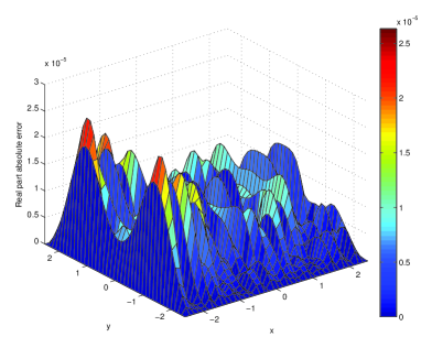
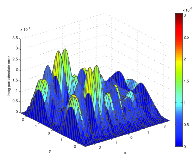
Figure 4: Surface plot of absolute error obtained for Test problem 2 with $N=25$ and $h=1/25$ (left panel for real part and right panel for imaginary part).

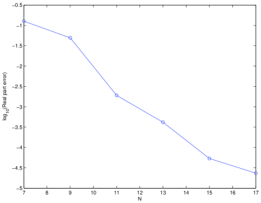
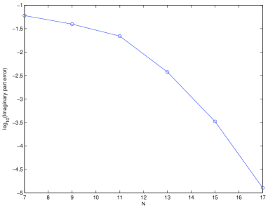
Figure 5: Exponential convergence in $N$ for Test problem 2 with $h=1/100$ (left panel for real part and right panel for imaginary part).

Table 5.1: Absolute errors for solving Test problem 2 with $N=25$ and $h=1/20$.

$t$	Maximum absolute error		Average absolute error
	Real part	Imaginary part	Real part	Imaginary part
0.10	5.5837e-05	7.2420e-05	5.2562e-06	6.5224e-06
0.25	1.1025e-04	1.6687e-04	1.3543e-05	1.2252e-05
0.50	6.4010e-05	6.5695e-05	1.8633e-05	1.8118e-05
0.75	6.6335e-05	8.7873e-05	1.8833e-05	1.8476e-05
1.00	8.9998e-05	9.2257e-05	1.4600e-05	1.6865e-05

Table 5.2: Absolute error for solving Test problem 2 by using the method of [1, Table 8] with $N_{x}=N_{y}=50$ and $\Delta t=1/20$.

t	Maximum absolute error		Average absolute error
	Real part	Imaginary part	Real part	Imaginary part
0.10	5.6517e-05	5.7493e-05	9.4025e-06	9.0740e-06
0.25	2.6182e-04	1.1500e-04	2.2048e-05	1.1013e-05
0.50	1.2792e-04	1.3972e-04	2.8362e-05	3.4913e-05
0.75	1.3312e-04	1.2511e-04	3.5252e-05	2.8212e-05
1.00	1.3647e-04	9.8227e-05	3.7975e-05	3.1640e-05

6 Concluding remarks

In the paper, we proposed a Galerkin-Legendre spectral method with implicit Runge-Kutta method for two-dimensional linear Schrödinger equation with the nonhomogeneous Dirichlet boundary conditions and initial condition. Optimal a priori error bounds are derived in the $L^{2}$-norm for the semidiscrete formulation. Our numerical results confirm the exponential convergence in space.

References

- [1] A. Mohebbi, M. Dehghan, The use of compact boundary value method for the solution of two-dimensional Schrödinger equation, J. Comput. Appl. Math. 225 (2009) 124–134.
- [2] R. Abdur, A. Ismail, Numerical studies on two-dimensional Schrödinger equation by chebyshev spectral collocation method, Sci. Bull. Politeh. Univ. Buchar. Ser. A 73 (2011) 101–110.
- [3] M. Dehghan, F. Emami-Naeini, The sinc-collocation and sinc-galerkin methods for solving the two-dimensional Schrödinger equation with nonhomogeneous boundary conditions, Appl. Math. Model. 73 (2013) 9379–9397.
- [4] M. Subasi, On the finite-difference schemes for the numerical solution of two dimensional Schrödinger equation, Numer. Methods Partial Differ. Equ. 18 (2002) 752–758.
- [5] X. Antoine, C. Besse, V. Mouysset, Numerical schemes for the simulation of the two-dimensional Schrödinger equation using non-reflecting boundary conditions, Math. Comput. 73 (2004) 1779–1799.
- [6] J. Kalita, P. Chhabra, S. Kumar, A semi-discrete higher order compact scheme for the unsteady two-dimensional Schrödinger equation, J. Comput Appl. Math. 197 (2006) 141–149.
- [7] M. Dehghan, A. Shokri, A numerical method for two-dimensional Schrödinger equation using collocation and radial basis functions, Comput. Math. Appl. 54 (2007) 136–146.
- [8] M. Dehghan, D. Mirzaei, The dual reciprocity boundary element method (DRBEM) for two-dimensional sine-Gordon equation, Comput. Methods Appl. Mech. Engrg. 197 (2008) 476–486.
- [9] Z. Tian, P. Yu, High-order compact adi (hoc-adi) method for solving unsteady 2d Schrödinger equation, Comput. Phys. Commun. 181 (2010) 861–868.
- [10] Z. Gao, S. Xie, Fourth-order alternating direction implicit compact finite difference schemes for two-dimensional Schrödinger equations, Appl. Numer. Math. 61 (2011) 593–614.
- [11] J. Shen, T. Tang, Spectral and High-Order Methods with Applications, Science Press, Beijing, 2006.
- [12] J. Shen, T. Tang, L.L. Wang, Spectral Methods: Algorithms, Analysis and Applications, Springer-Verlag, New York, 2011.
- [13] J. Shen, Efficient spectral-Galerkin method. I. Direct solvers of second- and fourth-order equations using Legendre polynomials, SIAM J. Sci. Comput. 15 (1994) 1489–1505.
- [14] J.L. Lions, E. Magenes, Non-Homogeneous Boundary Value Problems and Applications, Vol.I, Springer-Verlag, New York, 1972.
- [15] V. Thomée, Galerkin Finite Element Methods for Parabolic Problems, 2nd Ed, Springer-Verlag, Berlin Heidelberg, 2006.
- [16] W.H. Steeb, Problems and Solutions in Introductory and Advanced Matrix Calculus, World Scientific Publishing, London, 2006.
- [17] J.C. Butcher, Implicit Runge Kutta Processes, Math. Comp. 18 (1964) 50–64.
- [18] C. Canuto, M.Y. Hussaini, A. Quarteroni, T.A. Zang, Spectral Methods in Fluid Mechanics, Springer-Verlag, New York, 1988.