Anderson localization in metallic nanoparticle arrays

Abstract

Anderson localization has been observed in various types of waves, such as matter waves, optical waves and acoustic waves. Here we reveal that the effect of Anderson localization can be also induced in metallic nonlinear nanoparticle arrays excited by a random electrically driving field. We find that the dipole-induced nonlinearity results in ballistic expansion of dipole intensity during evolution; while the randomness of the external driving field can suppress such an expansion. Increasing the strength of randomness above the threshold value, a localized pattern of dipole intensity can be generated in the metallic nanoparticle arrays. By means of statistics, the mean intensity distribution of the dipoles reveals the formation of Anderson localization. We further show that the generated Anderson localization is highly confined, with its size down to the scale of incident wavelength. The reported results might facilitate the manipulations of electromagnetic fields in the scale of wavelength.
OCIS:(190.1450) Bistability; (190.6135) Spatial solitons; (250.5403) Plasmonics.

I Introduction

Anderson localization (AL) is a fundamental wave phenomenon that occurs in strongly disordered media anderson . In 1958, P. W. Anderson first suggested the possibility of electron localization inside a semiconductor, where the essential randomness is introduced anderson . To date, it has been reported that AL has been observed in various types of waves, such as matter wavesbilly ; roati ; ludlam ; chabe , optical waves scheffold ; schwartz ; karbasi2012 ; karbasi2013 , and acoustic waves hu .

Due to the diffraction limit of optical waves, the realization of optical AL at the extremely narrow scale is generally difficult to achieve in dielectric media, such as photonic lattices and optical fibres scheffold ; schwartz ; karbasi2012 ; karbasi2013 . However, it has been suggested that surface plasmon polaritons, which travel along a metal-dielectric interface, are a highly confined electromagnetic field with a size smaller than the wavelength. Therefore, to realize highly confined AL, an important candidate is based on plasmonics. Recently, the coupling plasmonic waveguide systemshi ; deng and the graphene plasmonic waveguide systemxu were proposed for producing the extremely narrow AL by introducing random potential into these waveguide systems.

It has been reported that the AL of electromagnetic polar waves in a random linear chain of dipoles has been studied PRB83 . In this work, we propose the realization of AL of surface plasmon polaritons in the arrays of metallic nanoparticles. Using a homogeneous electrically driving field, the nonlinear modulation instability and the bistability of optically induced dipoles in the metallic nanoparticle arrays have been studied in detail prl ; oe ; sr . Here, to realize AL of surface plasmon polaritons, a random electrically driving field, which has been used to create optical lattices with random perturbations schwartz , is utilized to excited the metallic nanoparticle arrays. Our numerical simulations demonstrate that the generated AL is highly confined, with its size down to the scale of incident wavelength.

The remainder of this paper is organized as follows. In section II, we introduce the nonlinearly coupling equations that describe the dynamics of particle’s dipoles excited by the external field in the arrays of metallic nanoparticles. In section III, we study the dynamics of the bright plasmonic dipole mode induced by the homogeneous driving field. In section IV, we investigate the generation of AL of dipole intensity by introducing the random electrically driving field. In section V, we investigate the size of the generated AL in the present system, finding that the size of the AL can be reduced to the scale of a wavelength of the excited field. The paper is concluded in section VI. The appendix presents the detailed parameters of the model.

II Model and basic equations

In the nanoparticle arrays, each spherical silver nanoparticle is arrayed linearly equidistant and embedded in a SiO₂ host, as shown in Fig. 1. The appendix presents the specific parameters of these silver nanoparticles. Surface plasmon polaritons could be excited by the electrical field imposed on these nanoparticle arrays, and the dynamics of such excited surface plasmon polaritons can be modelled using the following coupling equations prl ; oe ; sr

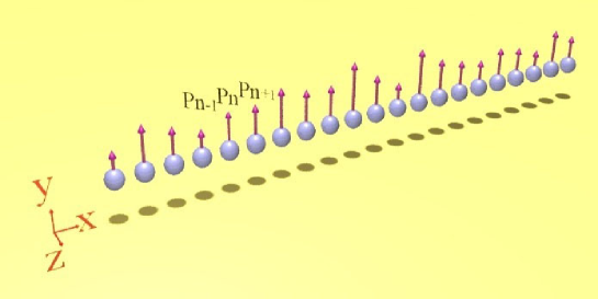
Figure 1: Schematic illustration of an array of spherical silver nanoparticles embedded in a SiO₂ host; the radius of the sphere is $a$, and the center-to-center distance of two adjacent particles is $d$. The dipoles are induced by an electrical driving field.

$$-i\frac{dP_{n}^{\perp}}{d\tau}+(-i\gamma+\Omega+|P_{n}|^{2})P_{n}^{\perp}+\sum_{m\neq n}G_{n,m}^{\perp}P_{m}^{\perp} = E_{n}^{\perp},$$ (1)

$$-i\frac{dP_{n}^{\parallel}}{d\tau}+(-i\gamma+\Omega+|P_{n}|^{2})P_{n}^{\parallel}+\sum_{m\neq n}G_{n,m}^{\parallel}P_{m}^{\parallel} = E_{n}^{\parallel},$$ (2)

where $P_{n}^{\bot,\parallel}=p_{n}^{\perp,\parallel}\sqrt{\chi^{(3)}}/(\sqrt{2(\varepsilon_{\infty}+2\varepsilon_{h})}\varepsilon_{h}a^{3})$ are the dimensionless slowly varying amplitudes of the vertical and parallel dipoles of the $n^{\mathrm{th}}$ particle, respectively. The indices ‘$\perp$’ and ‘$\parallel$’ represent the vertical and parallel directions with respect to the array axis, respectively. Thus, the total intensity of the dipole for the $n^{\mathrm{th}}$ particle is given as $|P_{n}|^{2}=|P_{n}^{\perp}|^{2}+|P_{n}^{\parallel}|^{2}$. $\gamma=\nu/(2\omega_{0})+(k_{0}a)^{3}\varepsilon_{h}/(\varepsilon_{\infty}+2\varepsilon_{h})$ is the scaled damping, with $k_{0}=\omega_{0}/c\sqrt{\varepsilon_{h}}$. $\Omega=(\omega-\omega_{0})/\omega_{0}$ is the detuning frequency of the dipoles. For a wavelength of $400nm$, $\Omega=0$. $\tau=\omega_{0}t$ is the scaled elapsed time. $E_{n}^{\perp,\parallel}=-3\varepsilon_{h}\sqrt{\chi^{(3)}}E_{n}^{ex,\perp,\parallel}/\sqrt{8(\varepsilon_{\infty}+2\varepsilon_{h})^{3}}$ represent the slowly varying amplitudes of the external optical fields in the respective directions. $G_{n,m}^{\perp,\parallel}$ is the linearly coupling parameter between the $n^{\mathrm{th}}$ and $m^{\mathrm{th}}$ particles in the corresponding directions and is induced by the long-range dipole-dipole interactions. According to prl , $G_{n,m}^{\perp,\parallel}$ can be expressed as follows:

$$G_{n,m}^{\perp} = \frac{\eta}{2}\left[(k_{0}d)^{2}-\frac{ik_{0}d}{|n-m|}-\frac{1}{|n-m|^{2}}\right]\frac{e^{-ik_{0}d|n-m|}}{|n-m|},$$ (3)

$$G_{n,m}^{\parallel} = \eta\left(\frac{ik_{0}d}{|n-m|}+\frac{1}{|n-m|^{2}}\right)\frac{e^{-ik_{0}d|n-m|}}{|n-m|},$$ (4)

where $\eta=\frac{3\varepsilon_{h}}{\varepsilon_{\infty}+2\varepsilon_{h}}(\frac{a}{d})^{3}$. Note that Eqs. (1) and (2) are suitable for cases of finite and infinite nanoparticle chains. The real-time evolution methods can be used to solve the $P_{n}$ in Eqs. (1) and (2).

For simplification, the optically induced dipole in the vertical direction (i.e., the character of ‘$\perp$’) is considered, while neglecting the induced dipole that is polarized along the parallel direction. Therefore, the dipole of the n^th particle can be written as $\mathbf{P}_{n}=(P^{\perp}_{n},P^{\parallel}_{n})=(P_{n},0)$. It was shown that in stationary conditions, the induced dipole exhibits a standard bistable curve that consists of three branches, namely, the low, middle, and top branchesoe . It was suggested that the dipole evolution dynamics is stable when the dipole is initially located at the low and top branches; however, it becomes unstable when the dipole is initially located at the middle branchoe .

III Dynamics of bright plasmonic dipole mode

We previously demonstrated that mai , using a homogeneous electrically driving field, a dipole kink could be formed when two adjacent particles’ dipole intensities were initially located at the low and top branches with respect to the bistable curve. Localized dipole modes could also be formed when two kinks were created in the nanoparticle arrays. As the intensity of the external field ($|E_{0}|^{2}$) is increased beyond the threshold, the kink begins to move, leading to the dipole intensity ($|Pv|^{2}$) jumping from the low branch to the top branch, thereby breaking the stability of the dipole mode mai .

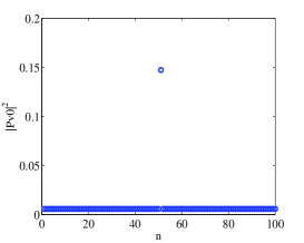
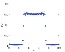
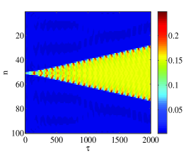
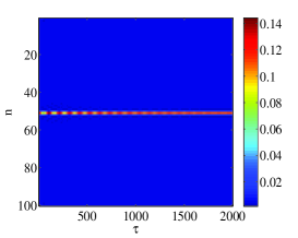
Figure 2: Bright plasmonic dipole mode in a 100-particle system excited by a homogeneous electric field of $|E_{0}|^{2}=0.90\times 10^{-4}$ under $\Omega=-0.1$ (the incident wavelength is approximately 440 nm): (a) initial dipole intensity at $\tau=0$, (b) dipole intensity at $\tau=2000$, (c) the evolution of the dipole intensity under and excitation of $|E_{0}|^{2}=0.90\times 10^{-4}$, and (d) the evolution of the dipole intensity under and excitation of $|E_{0}|^{2}=0.6\times 10^{-4}$, which is below the threshold value $|E_{c}|^{2}$.

Here we produce the bright dipole modes, as shown in Figs. 2(a)-2(c). As mentioned, this can be achieved by using the homogeneous external field and initially setting one of the particle’s dipole intensity at the top branch, while the other particle’s dipole is at the low branch. In our simulation, we set the external field as $|E_{0}|^{2}=0.90\times 10^{-4}$, and the direction of the driving field is vertical to the array direction. Figure 2(a) shows the corresponding initial state of the dipole intensities, while Fig. 2(b) illustrates the dipole intensity after the real-time evolution of $\tau=2000$. It clearly shows that the width of the bright dipole mode is broadening during the dipole evolution. This result means that, during the course of evolution, the dipoles of more particles jump from the low branch to the top branch. Figure 2(c) shows the real-time evolution of the dipole intensity. The blue-coloured area represents the intensity of dipoles that are located at the low branch, while the yellow-coloured area corresponds to the intensity of dipoles that are located at the top branch. The broadening behaviour of the dipole mode illustrated in Fig. 2(c) is similar to the motion of shock waves that was observed in the discrete nonlinear dissipative medium PRE62 . According to Ref. oe , the speed of the kink is related to $|E_{0}|^{2}$: the larger $|E_{0}|^{2}$ is, the faster is the speed of the kink. Additionally, note that there is a threshold of $|E_{0}|^{2}$ for the kink’s motion. In the present system, the threshold value can be achieved as $|E_{c}|^{2}=0.65\times 10^{-4}$. Below this threshold, the kink stops, as shown in Fig. 2(d).

IV Anderson localization of plasmonic dipole mode

To observe AL of surface plasmon polaritons in the present nanoparticle arrays, we introduce a random electrical driving field to excite the plasmonic dipoles. The external random electrical fields consist of a series of independent electrical fields. Each electrical field has a size of 40 nm and is successively imposed on the nanoparticle arrays. Note that such a narrow electrical driving field is achievable since recent work has reported that the size of the light spot can be reduced to a scale of less than 0.1$\lambda^{2}$ xiexiangsheng . By optimizing the system, as well as the modulations of optical field, a narrower light spot is expected xie2014 .

In the simulations, the varying range of the external driving fields that are imposed on the 100-particle system is set as $|E_{0}|^{2}=0.45\times 10^{-4}\sim 1.35\times 10^{-4}$. It was demonstrated that the induced dipole intensity relies on the intensity of the driving field mai . Therefore, for a random electrical driving field, the induced dipole intensity of each particle is different from that induced from other particles. Hence, the excited dipoles of the nanoparticle arrays can be considered as a random system, which provides possibility for the generation of localized dipole modes. To observe this effect, the dipole intensity of the middle nanoparticle is set to the top branch; see Fig. 3(a), while the dipole intensities of the other nanoparticles are located at the low branch. Figure 3(b) depicts the intensity distribution after the real-time evolution of $\tau=2000$. Figure 3(c) shows the evolution dynamics of the dipole intensity. It shows that the pattern still broadens in the short stage, but it becomes localized for a longer propagation stage, indicating the formation of a stable localized bright dipole mode. This behaviour is very different from that observed in Figs. 2(a)-2(c). We attribute this phenomenon of a localized pattern to the introduction of a random electrical driving field. Owing to the randomness of the driving field, for the driving intensity $|E_{0}|^{2}$ below the threshold, the dipole-induced nonlinearity is negligible, and the dipole evolution becomes stable, which helps to suppress the expansion of dipole intensity.

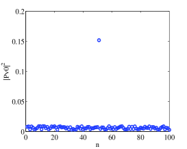
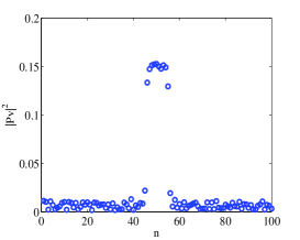
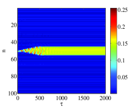
Figure 3: Localized plasmonic dipole mode in a 100-particle system excited by the random electrical driving field under $\Omega=-0.1$: (a) initial dipole intensity distribution at $\tau=0$, (b) the dipole intensity distribution at $\tau=2000$, and (c) the evolution of dipole intensity.

To investigate the influence of statistical regularities of the random electrical driving field on the formation of localized dipole modes, we perform 200 real-time evolutions of dipole modes excited by the random electrical field. For each real-time simulation, the electrical field imposed on the nanoparticles is different, but the varying range of the driving field is kept the same, i.e., set as $|E_{0}|^{2}=0.45\times 10^{-4}\sim 1.35\times 10^{-4}$. In this case, we can observe through simulations the phenomenon of AL of the surface plasmon polaritons, as evident in Fig. 4. Figure 4(a) shows the mean value of the dipole intensity after real-time evolution at $\tau=2000$, with the detuning parameter set as $\Omega=-0.1$. The blue scattered circle denotes the calculated mean dipole intensity at $\tau=2000$; while the red solid curve shows the fitting results. Figure 4(b) illustrates the evolution of the dipole intensity modes. Both Figs. 4(a) and 4(b) clearly depict a nice localized dipole mode, i.e., Anderson localization. Note that Fig. 4 is the statistical results after 200 real-time evolutions, but each simulation, e.g., see Fig. 3, can produce a localized dipole pattern. We should point out that the observed localized pattern shown in Fig. 4 is not caused by the dipole-induced nonlinearity. This can be verified by the results shown in Fig. 2. Due to the randomness of the driving field, for the driving intensity below the threshold value, the dipole intensity $|P_{v}|^{2}$ is invariant with time (it is stable during evolution). Under this circumstance, the nonlinear model described by Eqs. (1) and (2) can be reduced to a linear system. As a result, the randomness of the driving field, as well as the long-range dipole-dipole interactions, helps to suppress the dipole expansion, eventually leading to Anderson localization.

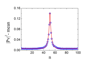
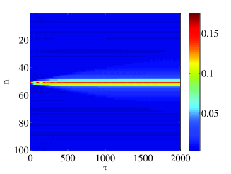
Figure 4: The statistical results of 200 real-time evolutions of dipole intensity excited by the random electrical driving field under $\Omega=-0.1$. The varying range intensity of the random driving field for each simulation is kept the same, i.e., set as $|E_{0}|^{2}=0.45\times 10^{-4}\sim 1.35\times 10^{-4}$: (a) Mean distribution of dipole intensity at $\tau=2000$. The blue circles denote the calculated mean value; while the red curve represents the fitting result of $0.14exp[\pm(x-51)/2.5]+0.007$. (b) The evolution dynamics of the mean dipole intensity.

Next, we investigate the relation between the strength of randomness of the electrical driving field and the formation of AL. For this purpose, a random factor $\kappa$ that describes the strength of the randomness is introduced, as follows:

$${\left|E\right|}^{2}={\left|E_{0}\right|}^{2}\pm\kappa{\left|E_{0}\right|}^{2},$$ (5)

Equation (5) indicates that the electrical driving field varies from ${\left|E_{0}\right|}^{2}-\kappa{\left|E_{0}\right|}^{2}$ to ${\left|E_{0}\right|}^{2}+\kappa{\left|E_{0}\right|}^{2}$. Increasing the value of $\kappa$ will broaden the varying range of the random electrical driving field, and hence enhances the strength of the randomness. As a result, the probability that the intensity of the driving field is below the threshold intensity $|E_{c}|^{2}$ is also increased.

To observe the effect of $\kappa$ on the formation of AL, we perform simulations with different values of $\kappa$, as shown in Fig. 5. Figures 5(a)-5(c) present the results of a single real-time evolution with (a) $\kappa$=0.2, (b) $\kappa$=0.4, and (c) $\kappa$=0.6, respectively. From Figs. 5(a)-5(c), we can observe that the width of the bright plasmonic dipole mode decreases as the strength of the randomness $\kappa$ increases. In particular, for the case of $\kappa=0.4,0.6$, see Figs. 5(b) and 5(c), we can observe the formation of a stable localized dipole pattern. To observe the phenomenon of AL, we perform the statistical calculation of such dipole intensity after 200 real-time evolutions, keeping the parameter $\kappa$ unchanged. The mean values of the statistical results are shown in Figs. 5(d)-5(f). From these numerical results, it is shown that the effect of AL becomes stronger with a larger $\kappa$. Note that for each real-time simulation, an evolved localized pattern induced by the random electrical field was observed, e.g., see Fig. 3. However, by means of statistics, the mean intensity distribution of $|Pv|^{2}$ after 200 real-time simulations reveals the phenomenon of AL, as shown in Fig. 5. Furthermore, it is shown that for a larger $\kappa$, the probability that the external driving intensity is less than the threshold value becomes larger, which leads to a narrower localized pattern.

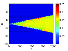
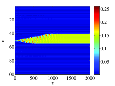
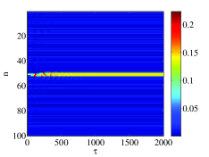
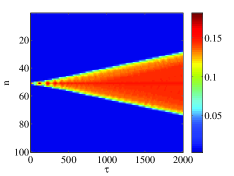
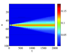
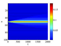
Figure 5: (a)$\sim$(c) The evolution of dipole intensity in a 100-particle system excited by the random electrical driving field under $\Omega=-0.1$, $|E_{0}|^{2}=0.9\times 10^{-4}$: (a) $\kappa=0.2$, (b) $\kappa=0.4$, and (c) $\kappa=0.6$. (d)$\sim$(f) The corresponding statistical results for (a)$\sim$(c) after 200 real-time evolutions: (d) $\kappa=0.2$, (e) $\kappa=0.4$, and (f) $\kappa=0.6$.

V Extremely narrow Anderson localization

We further study the effect of $\kappa$ on the size of the Anderson-localized dipole mode. Here, we introduce the formula for calculating the width of the dipole mode, which is written as

$$W=\frac{\left(\sum^{N}_{n=1}{\left|P_{n}\right|}^{2}\right)^{2}}{\sum^{N}_{n=1}{\left|P_{n}\right|}^{4}},$$ (6)

where $W$ denotes the width of the localized mode, and $N$ the number of nanoparticles. Note that in the finite nanoparticle array, the value of the dipole that is located at the low branch is not zero, which would give rise to calculation errors when using Eq. (6). To eliminate this error, ${P_{n}}$ should be rescaled by reducing the average value of the dipole intensity that is located at the low branch.

Using equation (6), we can obtain the relation between $W$ and $\kappa$, as shown in Fig. 6. The employed parameters are the same as those shown in Fig. 5. Both Figs. 6(a) and 6(b) show that with a larger value of $\kappa$, the value of $W$ becomes smaller, suggesting that the statistical width of the localized dipole patterns becomes narrower. In particular, in the case of $\kappa=0.6$, the statistical width of the dipole mode is approximately 7 particles (200 nm), which is in the scale of one incident wavelength, as shown from the violet curve in Fig. 6(b). The generated extremely narrow localized dipole mode in nanoparticle arrays may have potential applications in highly precise detection and manipulation of electromagnetic fields.

Further, it is interesting to find that there exists a threshold value $\kappa_{c}$, above which the AL of the dipole intensity can be generated, and below which the ballistic expansion of the dipole intensity occurs. The existence of $\kappa_{c}$ is resulted from the fact that there is a critical driving intensity $|E_{c}|^{2}$ for the kink moving. To generated localized patterns, the lower limiting value $|E_{0}|^{2}-\kappa|E_{0}|^{2}$ of the random driving intensity should be less than $|E_{c}|^{2}$. Based on this relation, we can find $\kappa_{c}=0.278$. Therefore, for the cases of $\kappa=0$ and $\kappa=0.2$, we cannot obtain the localized patterns, as shown in Figs. 5(a) and 5(d) and Fig. 6(b); while for the cases of $\kappa=0.4$ and $\kappa=0.6$, the localized patterns can be generated, as shown in Fig. 5 and Fig. 6.

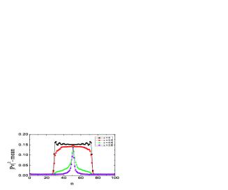
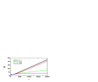
Figure 6: The statistical results of 200 real-time simulations with different values of $\kappa$. The detuning is set as $\Omega=-0.1$. (a) The distribution of mean value of the dipole intensity at $\tau=2000$; (b) the width evolution of localized dipole modes for different values of $\kappa$.

Obviously, $\kappa_{c}$ strongly relies on the external driving intensity $|E_{0}|^{2}$, as well as the critical driving intensity $|E_{c}|^{2}$ that is determined by the structural parameters, such as the radius of the metal sphere and the distance between two adjacent particles. For the present system we considered here (i.e., the critical driving intensity is fixed to $|E_{c}|^{2}=0.65\times 10^{-4}$), the relation between $\kappa_{c}$ and $|E_{0}|^{2}$ can be determined by the expression $|E_{0}|^{2}-\kappa_{c}|E_{0}|^{2}=|E_{c}|^{2}$, with the result shown in Fig. 7. Figure 7 shows that increasing $|E_{0}|^{2}$ can also increases $\kappa_{c}$. This phenomenon can be understood as the following: the increase of the electrical driving intensity would strengthen the dipole-induced nonlinearity, and hence the expansion of the dipole intensity. As a result, to observe the localized modes, a stronger randomness (i.e., with a larger $\kappa$) of the electrical driving field is required.

Figure 7: The relation between $\kappa_{c}$ and the middle value of random external field($|E_{0}|^{2}$) with the same settings as discussed above.

VI Conclusion

In conclusion, we performed numerical analysis of Anderson localization of surface plasmon polaritons in a finite nonlinear nanoparticle array. Unlike the conventional Anderson localization, which is generally based on the structural disorder in a medium, here the random electrical driving field was utilized to excite the Anderson-localized patterns. It was shown that the dipole-induced nonlinearity results in ballistic expansion of dipole intensity; while the randomness of the external driving field can suppress such an expansion. Our numerical simulations by means of statistics confirmed that the effect of Anderson localization can be generated. We further demonstrated that the generated Anderson localization is highly confined, with its size down to the scale of one incident wavelength. Our results might provide a new scheme for the manipulations of electromagnetic fields in the scale of wavelength.

The possibility for experimentally generating the Anderson-localized dipole mode can be enhanced by reasonably adjusting the structure parameters such as increasing the radius of particle, as well as the center-to-center distance between two adjacent particles. Moreover, it is also possible to consider the random cell that contains two or more particles, which would significantly alleviate the requirements of driving field.

Parameters The radius of the nanoparticle is fixed to $a=10$ nm, and the distance between two adjacent particles is fixed to $d=30$ nm. An external optical field is launched into the host and the dipole of the particles is excited. The dispersion of the host can be neglected because the permittivity of SiO₂ is nearly $\varepsilon_{h}\simeq 2.15$ for the optical wavelength range. The linear part of the dielectric constant of the silver particle follows the Drude model, which can be expressed as $\varepsilon_{\mathrm{Ag}}^{\mathrm{L}}=\varepsilon_{\infty}-\omega_{P}^{2}/[\omega(\omega-i\nu)]$, where $\varepsilon_{\infty}=4.96$, $\hbar\omega_{P}=9.54$ eV and $\hbar\nu$=0.055 eV oe18 . The nonlinear part of the dielectric constant is selected as the standard cubic type, which can be obtained as $\varepsilon_{\mathrm{Ag}}^{\mathrm{NL}}=\chi^{(3)}|E_{n}|^{2}$, where $\chi^{(3)}\simeq 3\times 10^{-9}$ esu for the silver spheres with a radius of 10 nmoe20 , and $E_{n}$ is the local field inside the $n^{\mathrm{th}}$ particle. The frequency of the surface plasmon resonance of the silver nanoparticles, namely, $\omega_{0}$, can be expressed as $\omega_{0}=\omega_{P}/\sqrt{\varepsilon_{\infty}+2\varepsilon_{h}}$.

References

- (1) P. W. Anderson, “Absence of Diffusion in Certain Random Lattices,” Phys. Rev. 109, 1492-1505 (1958).
- (2) J. Billy, V. Josse, Z. Zuo, A. Bernard , B. Hambrecht, P. Lugan, D. Clément, L. Sanchez-Palencia, P. Bouyer, and A. Aspect, “Direct observation of Anderson localization of matter waves in a controlled disorder,” Nature 453, 891-894 (2008).
- (3) G. Roati, C. D’Errico, L. Fallani, M. Fattori, C. Fort, M. Zaccanti, G. Modugno, M. Modugno, and M. Inguscio, “Anderson localization of a non-interacting Bose-Einstein condensate,” Nature, 453, 895-898 (2008).
- (4) J. J. Ludlam, S. N. Taraskin, S. R. Elliott, and D. A. Drabold, “Universal features of localized eigenstates in disordered systems,” 17, 321-327 (2005).
- (5) J. Chabé, G. Lemarié, B. Grémaud, D. Delande, P. Szriftgiser, and J. C. Garreau, “Experimental Observation of the Anderson Metal-Insulator Transition with Atomic Matter Waves,” Phys. Rev. Lett. 101, 1-30 (2008).
- (6) F. Scheffold, R. Lenke, R. Tweer and G. Maret, “Localization or classical diffusion of light,” Nature 398, 206-207 (1999).
- (7) T. Schwartz, G. Bartal, S. Fishman and M. Segev, “Transport and Anderson localization in disordered two-dimensional photonic lattices,” Nature 446, 52-55 (2007).
- (8) S. Karbasi, C. R. Mirr, P. G. Yarandi, R. J. Frazier, K. W. Koch and A. Mafi, “Observation of transverse Anderson localization in an optical fiber,” Opt. Lett. 37, 2304-2306 (2012).
- (9) S. Karbasi, R. J. Frazier, K. W. Koch, T. Hawkins, J. Ballato and A. Mafi, “Image transport through a disordered optical fibre mediated by transverse Anderson localization,” Nat. Commun. 5, 163-180 (2013).
- (10) H. Hu, A. Strybulevych, J. H. Page, S. E. Skipetrov and B. A. V. Tiggelen, “Localization of ultrasound in a three-dimensional elastic network,” Nature Phys. 4, 945-948 (2008).
- (11) H. Deng, F. Ye, B. A. Malomed, X. Chen, and N. C. Panoiu, “Optically and electrically tunable dirac points and zitterbewegung in graphene-Based photonic superlattices,” Phys. Rev. B 91, 201402 (2015).
- (12) H. Deng, X. Chen, B. A. Malomed, N. C. Panoiu and F. Ye, “Transverse Anderson localization of light near Dirac points of photonic nanostructures,” Sci. Rep. 5, 15585 (2015).
- (13) Y. Xu and H. D. Deng, “Tunable Anderson localization in disorder graphene sheet arrays,” Opt. Lett. 41, 567-570 (2016).
- (14) S. Faez, A. Lagendijk, and A. Ossipov, “Critical scaling of polarization waves on a heterogeneous chain of resonators,” Phys. Rev. B, 83, 210-216 (2010).
- (15) R. E. Noskov, P. A. Belov and Y. S. Kivshar, “Subwavelength modulational instability and plasmon oscillons in nanoparticle arrays,” Phys. Rev. Lett. 108, 324-329 (2012).
- (16) R. E. Noskov, P. A. Belov and Y. S. Kivshar, “Subwavelength plasmonic kinks in arrays of metallic nanoparticles,” Opt. Express, 20, 2733-2739 (2012).
- (17) R. E. Noskov, P. A. Belov and Y. S. Kivshar, “Oscillons, soltions, and domain walls in arrays of nonlinear plasmonic nanoparticles,” Sci. Rep. 2, 873 (2012).
- (18) Z. Mai, S. Fu, Y. Li, X. Zhu, Y. Liu and J. Li, “Control of the stability and soliton formation of dipole moments in a nonlinear plasmonic finite nanoparticle array,” Photonics Nanostruct.Fundam. Appl. 13, 42-49 (2015).
- (19) M. Salerno, B. A. Malomed, and V. V. Konotop, “Shock wave dynamics in a discrete nonlinear Schrodinger equation with internal losses,” Phys. Rev. E, 62, 8651-8656 (2000).
- (20) L. Yang, X. Xie, S. Wang and J. Zhou, “Minimized spot of annular radially polarized focusing beam,” Opt. Lett. 38, 1331-1333 (2013).
- (21) X. Xie, Y. Chen, K. Yang, and J. Zhou, “Harnessing the point-spread function for high-resolution far-field optical microscopy,” Phys. Rev. Lett. 113, 263901 (2014).
- (22) P. B. Johnson and R. W. Christy, “Optical constants of the noble metals,” Phys. Rev. B, 6, 4370-4379 (1972).
- (23) V. P. Drachev, A. K. Buin, H. Nakotte and V. M. Shalaev, “Size dependent for conduction electrons in Ag nanoparticles,” Nano Lett. 4, 1535-1539 (2004).