Abstract

We study sine polynomials of the form

$$\kappa\,\sin(x)+\sum_{k=2}^{n-1}\sin(kx)+\lambda\,\sin(nx)\qquad(\kappa,\lambda\in\mathbb{R})$$

that is nonnegative for all $x\in[0,\pi]$. These include, in particular,

$$\frac{5}{4}\,\sin(x)+\sum_{k=2}^{n-1}\sin(kx)+\frac{2n-3}{4n}\,\sin(nx))\qquad(n\mbox{ odd }),$$

and

$$\left(n+\frac{1}{2}\right)\,\sin(x)+\sum_{k=2}^{n}\sin(kx)\hskip 68.2866pt(n\mbox{ even }).$$

We also characterize all nonnegative sine polynomials of degree 3 and all nonnegative cosine polynomials of degree 2.

Mathematics Subject Classification (2010). 26D05, 42A05.

Keywords. Trigonometric sums, positivity, inequalities, symbolic computation.

Acknowledgments. This research was inspired while the author was visiting the National Center for Theoretical Sciences (No. 1 Sec. 4 Roosevelt Rd., National Taiwan University, Taipei, 106, Taiwan) in January, 2016. The author is grateful for the support and hospitality of the Center.

The research of this author is partially supported by the Hong Kong Government GRF Grant PolyU 5012/10P and the Hong Kong Polytechnic University Grants G-YK49 and G-U751.

1 Introduction

Nonnegative trigonometric polynomials are useful. Many excellent surveys on their history and applications are available in the literature. See, for example, Brown [3], Dumitrescu [4], and Koumandos [6], and the many references therein.

Notations. For convenience, we adopt the following notations:

$$c_{k}=c(k):=\cos(kx)\,,$$

$$s_{k}=s(k):=\sin(kx)\,,$$

$$[a_{1},a_{2},...,a_{n}]_{s}:=\sum_{k=1}^{n}a_{k}s_{k}\,,$$

$$[a_{0},a_{1},...,a_{n}]_{c}:=\sum_{k=0}^{n}a_{k}c_{k}\,,$$

where $\left\{a_{k}\right\}_{1}^{n}$ is a given sequence of real numbers. We use the acronym NN as an abbreviation for either the adjective “nonnegative” or the “property of being nonnegative”, depending on the context. The property usually concerns an expression depending on some variable $x$ in some interval $I$. When the interval $I$ is not explicitly specified, the default is $[0,\pi]$. We also abbrviate “lefthand (righthand) side” to RHS (LHS).

In 1958, Vietoris [11] proved a deep result concerning NN trigonometric polynomials. It was improved by Belov [2] in 1995.

Theorem 1 (Vietoris-Belov).

Suppose that $\left\{a_{k}\right\}_{0}^{\infty}$ is a sequence of non-increasing positive numbers satisfying the condition

$$\sum_{k=1}^{m}(-1)^{k-1}k\,a_{k}\geq 0,\quad\mbox{ for all (even) }m\geq 1.$$

Then for all $x\in[0,\pi]$ and $m\geq 1$,

$$\sum_{k=0}^{m}a_{k}\,c_{k}\geq 0\qquad\mbox{ and }\qquad\sum_{k=1}^{m}a_{k}\,s_{k}\geq 0.$$

For sine polynomials with $a_{k}\searrow$, (B) is also necessary for all its partial sums to be NN.

Remark 1.

Frequently, Theorem 1 is applied to a finite sequence $\left\{a_{k}\,:\,k\leq n\right\}$ (simply take $a_{k}=0$ for $k>n$). The length of the sequence $n$ is called the degree of the trigonometric polynomial. Then (B) consists of $\frac{n}{2}$ (if $n$ is even) or $\frac{n-1}{2}$ inequalities. ∎

Remark 2.

The original Vietoris result covers a smaller family of polynomials including

$\hskip 56.9055pta_{0}=a_{1}=1,\qquad\textstyle a_{2k+1}=a_{2k}=\frac{1\cdot 3\cdot 5\cdots(2k-1)}{2\cdot 4\cdot 6\cdots(2k)}\quad(k=1,2,...).$ ∎

Remark 3.

Vietoris’ (but not Belov’s) result has recently been extended by the author [9] to sine polynomials with non-decreasing and non-decaying coefficients. ∎

Contrast Theorem 1 with the following NN criterion, due to Fejér [5], in which only the NN of the entire polynomial, not its partial sums, is asserted.

Theorem 2 (Fejér).

Suppose $a_{k}\searrow$, ${}>0$, $k\leq n$, satisfy

$$a_{k}+a_{k+2}\geq 2a_{k+1},\qquad k=1,2,...,n-2.$$

Then

$$\sum_{k=1}^{n-1}a_{k}\,s_{k}+\frac{a_{n}}{2}\,s_{n}\quad\mbox{ is NN in }[0,\pi].$$

Remark 4.

Among the simplest examples are $[n,n-1,n-2,...,1]_{s}$ (attributed to E. Lukács by Fejér [5]) and

$$\sigma(x)=[\,1,1,...,1,\textstyle\frac{1}{2}\,]_{s}.$$ (1.1)

None of their proper partial sums are NN.

New NN polynomials can be constructed by taking positive linear combinations of known ones. For instance,

$$[2,1]_{s}+[2,2,2,2,1]_{s}=[4,3,2,2,1]_{s}$$

is NN; but it satisfies neither Theorem 1 nor Theorem 2. ∎

Remark 5.

Strangely enough, no cosine analog of Theorem 2 is known. ∎

A long term goal of the author is to establish general NN criteria that extend or unify these known results. In the meantime, the discovery of new families of NN polynomials will help to achieve that goal. It is the purpose of this article to present such a new family that includes $\sigma$ as a particular case.

In Section 2, we show that, for odd $n$,

$$\phi(x)=\textstyle[\frac{5}{4},1,1,\cdots,1,\frac{2n-3}{4}]_{s},$$ (1.2)

is NN. Here, all the middle coefficients are 1. The proof is non-trivial. In Section 3, we consider polynomials of the more general form $[\kappa,1,1,\cdots,1,\lambda]_{s}$.

Remark 6.

Belov’s criterion (B) imposes multiple inequalities on the coefficients and reaps multiple (all partial sums) NN results. It is natural to wonder whether imposing only a single inequality, namely, the $n$-th one (i.e. (1.5) below), can lead to any useful conclusion. It turns out that (1.5) alone is not enough to guarantee NN. However, it is known that (1.5) is necessary for NN. In fact, the following more general assertion holds. ∎

Proposition 3.

Let $\left\{a_{k}\right\}_{1}^{n}$ be a finite sequence of real numbers, positive or negative.

1. A necessary condition for $[a_{1},...,a_{n}]_{s}$ to be NN in a right neighborhood of $x=0$ is

   $$\sum_{k=1}^{n}ka_{k}\geq 0.$$ (1.3)

   In case it is known that $\sum ka_{k}=0$, an additional necessary condition is

   $$\sum_{k=1}^{n}k^{3}a_{k}\leq 0.$$ (1.4)

2. A necessary condition for $[a_{1},...,a_{n}]_{s}$ to be NN in a left neighborhood of $x=\pi$ is

   $$\sum_{k=1}^{n}\,(-1)^{k+1}ka_{k}\geq 0.$$ (1.5)

   In case it is known that

   $$\sum\,(-1)^{k+1}ka_{k}=0,$$ (1.6)

   an additional necessary condition is

   $$\sum_{k=1}^{n}\,(-1)^{k+1}k^{3}a_{k}\leq 0.$$ (1.7)

[In an earlier version, (1.4) and (1.6) had the typo where $\leq$ was mistakenly typed as $\geq$.]

Proof. We only give the proof of (i), that of (ii) being similar. Denote $f(x)=\sum a_{k}s_{k}.$ Since $f(0)=0$ and $f(x)\geq 0$ for $x\in(0,\epsilon)$ for some $\epsilon>0$, we have $f^{\prime}(0)\geq 0$. Note that $f^{\prime}(x)=\sum ka_{k}c_{k}$. Substituting $x=0$ in this identity gives (1.3).

If it happens that $\sum ka_{k}=0$, then $f^{\prime}(0)=0$. Note that $f^{\prime\prime}(x)=-\sum k^{2}a_{k}s_{k}$ and $f^{\prime\prime\prime}(x)=-\sum k^{3}a_{k}c_{k}$. Hence, $f^{\prime\prime}(0)=0$ and $f^{\prime\prime\prime}(0)=-\sum k^{3}a_{k}$. The only way that $f(x)$ can be NN in $(0,\epsilon)$ is to have $f^{\prime\prime\prime}(0)\geq 0$, yielding the desired necessary condition (1.4).   

Remark 7.

$\sigma$ of (1.1) satisfies (1.6) and (1.7) when $n$ is even. When $n$ is odd, it satisfies (1.5) with strict inequality. On the other hand, $\phi$ of (1.2) satisfies (1.6) and (1.7) (with equality) when $n$ is odd (see (3.6) below). ∎

Remark 8.

It is easy to show that, after replacing $\geq$ by $>$, condition (1.3) (or (1.5)) is sufficient for the sine polynomial to be NN in some right (left) neighborhood of $x=0$ ($x=\pi$). However, this simple fact is not too useful because there is no information on how large this neighborhood can be. ∎

We will make use of the well-known inequalities (for $t\geq 0$)

$$\hskip 56.9055pt\sin(t)\leq t,\qquad\cos(t)\geq 1-\frac{t^{2}}{2}$$ (1.8)

$$\hskip 62.59605ptt-\frac{t^{3}}{6}\,\,\leq\,\,\sin(t)\,\,\leq\,\,t-\frac{t^{3}}{6}+\frac{t^{5}}{120}$$ (1.9)

$$1-\frac{t^{2}}{2}+\frac{t^{4}}{24}-\frac{t^{6}}{720}\,\,\leq\,\,\cos(t)\,\,\leq\,\,1-\frac{t^{2}}{2}+\frac{t^{4}}{24}$$ (1.10)

in the next section. These can be proved by iteratively integrating the simple inequality $\cos(t)\leq 1$. The polynomials involved are truncated Taylor series of $\sin$ and $\cos$, respectively.

The Sturm procedure is a useful technique for proving the NN of specific trigonometric polynomials with given constant coefficients. In a nutshell, the NN of a given trigonometric polynomial is equivalent to that of a corresponding algebraic polynomial. The latter can be verified using the classical Sturm result on the exact number of real solutions of an algebraic polynomial in a given interval of real numbers, with the help of a computer software. In our study, we used the extremely helpful mathematical software MAPLE 2016. Detailed expositions can be found in [9], [1], and [10].

2 $\phi=[\,\frac{5}{4},1,1,...,1,\frac{2n-3}{4n}\,]_{s}\,$, $n\geq 3$, Odd

Other than the first and last, all coefficients of $\phi$ are 1.

Lemma 1.

For odd $n\geq 3$, $\phi$ is NN in $[0,\pi]$.

Proof. The Sturm procedure have been used to confirm the conclusion for $n=3,5,7$, and $9$. In the following, we assume that $n\geq 11$.

In $\big{[}0,\frac{\pi}{n}\big{]}$, all terms of the polynomial in question are NN. Hence, the sum is positive. It remains to establish NN in the remaining interval $\big{[}\frac{\pi}{n},\pi\big{]}$. By applying the reflection $x\mapsto\pi-x$, we see that this is equivalent to the NN, in $\big{[}0,\pi-\frac{\pi}{n}\big{]}$, of

$$\textstyle S_{1}=\left[\,\frac{5}{4},-1,1,-1,1,...\,,-1,\frac{2n-3}{4n}\,\right]_{s}.$$

The product-to-sum identity gives

$$8c{\textstyle\left(\frac{1}{2}\right)}S_{1} = 5s{\textstyle\left(\frac{1}{2}\right)}+s{\textstyle\left(\frac{3}{2}\right)}-\frac{2n+3}{n}\,s{\textstyle\left(n-\frac{1}{2}\right)}+\frac{2n-3}{n}\,s{\textstyle\left(n+\frac{1}{2}\right)}$$ (2.1)

$$= 5s{\textstyle\left(\frac{1}{2}\right)}+s{\textstyle\left(\frac{3}{2}\right)}+4s{\textstyle\left(\frac{1}{2}\right)}c(n)-\frac{6}{n}\,c{\textstyle\left(\frac{1}{2}\right)}s(n).$$

By substituting $2x$ for $x$ in (2.1), we see that the desired assertion is the same as the NN of

$$S_{2}=5s_{1}+s_{3}+4s_{1}c_{2n}-\frac{6}{n}\,c_{1}s_{2n}$$ (2.2)

in $\big{[}0,\frac{\pi}{2}-\frac{\pi}{2n}\big{]}$. We establish this claim separately in each of five subintervals:

$$\bigcup_{k=1}^{5}I_{k}=[\,0.14,1.4\,]\cup\big{[}1.4,{\textstyle\frac{\pi}{2}-\frac{\pi}{2n}\big{]}\cup\big{[}\frac{\pi}{2n},0.14\big{]}\cup\big{[}\frac{\pi}{4n},\frac{\pi}{2n}\big{]}\cup\big{[}0,\frac{\pi}{4n}\big{]}.}$$ (2.3)

The following numbered paragraphs correspond to these subintervals in the same order.

1. Since $c_{2n}\leq 1$ and $s_{2n}\leq 1$, (2.2) yields

   $$S_{2}\geq S_{3}:=s_{1}+s_{3}-\frac{6}{n}\,c_{1},$$ (2.4)

   for all $n$. In particular, with the choice $n=11$,

   $$S_{2}\geq s_{1}+s_{3}-\frac{6}{11}\,c_{1}.$$ (2.5)

   Using the Sturm procedure for general trigonometric polynomials, as described in [10], we can verify that the RHS of (2.5) is NN in $I_{1}$.

2. Differentiating (2.4) gives

   $$S_{3}^{\prime}(x)=c_{1}+3\,c_{3}+\frac{6}{n}\,s_{1}.$$ (2.6)

   At $x=\frac{\pi}{2}-\frac{\pi}{2n}$,

   $$S_{3}^{\prime} = \sin{\textstyle\left(\frac{\pi}{2n}\right)}-3\,\sin{\textstyle\left(\frac{3\pi}{2n}\right)}+\frac{6}{n}\,\cos{\textstyle\left(\frac{\pi}{2n}\right)}$$ (2.7)

   $$\leq \sin{\textstyle\left(\frac{\pi}{2n}\right)}-3\,\sin{\textstyle\left(\frac{3\pi}{2n}\right)}+\frac{6}{n}\,.$$

   Using the first inequality of (1.8) for the first term and the LHS of (1.9) for the second term, we can show that the last expression of (2.7) is ${}\leq 0$, implying that $S_{3}^{\prime}\big{(}\frac{\pi}{2}-\frac{\pi}{2n}\big{)}\leq 0$. Differentiating (2.6) gives

   $$S_{3}^{\prime\prime}(x)=(-s_{1}-9s_{3})+\frac{6}{n}\,c_{1}.$$

   In $I_{2}$, the two terms in the RHS of the above expression are nonnegative. Thus, $S_{3}^{\prime\prime}(x)>0$, implying that $S_{3}^{\prime}$ is increasing in this interval. Consequently, $S_{3}^{\prime}$ is nonnegative in $I_{2}$, implying that $S_{3}$ is decreasing there. At the right endpoint,

   $$S_{3} = \cos{\textstyle\left(\frac{\pi}{2n}\right)}-\cos{\textstyle\left(\frac{3\pi}{2n}\right)}-\frac{6}{n}\,\sin{\textstyle\left(\frac{\pi}{2n}\right)}$$ (2.8)

   $$\geq \cos{\textstyle\left(\frac{\pi}{2n}\right)}-\cos{\textstyle\left(\frac{3\pi}{2n}\right)}-\frac{3\pi}{n^{2}}\,.$$

   Using the appropriate inequality of (1.8) for the first terms and of (1.10) for the second term, we can show that the expression in the second line of (2.8) is NN. Hence, $S_{3}$ is NN at $x=\frac{\pi}{2}-\frac{\pi}{2n}$. Since $S_{3}$ is decreasing, it is NN in $I_{2}$. By (2.4), $S_{2}$ is NN in the same interval.

3. Using (2.6), we can easily verify that $S_{3}$ is increasing in $[0,0.14]$. At $x=\frac{\pi}{2n}$,

   $$S_{3} = \sin{\textstyle\left(\frac{\pi}{2n}\right)}+\sin{\textstyle\left(\frac{3\pi}{2n}\right)}-\frac{6}{n}\,\cos{\textstyle\left(\frac{\pi}{2n}\right)}$$

   $$\geq \sin{\textstyle\left(\frac{\pi}{2n}\right)}+\sin{\textstyle\left(\frac{3\pi}{2n}\right)}-\frac{6}{n}\,.$$

   Using (1.8), we can show that the last expression, and hence, also $S_{3}$ is NN.

4. We estimate the first two terms in (2.2) using (1.9):

   $$5\,s_{1}+s_{3}\geq 8x-\frac{16}{3}\,x^{3}.$$

   In this interval, the third term in (2.2) is ${}\leq 0$, and

   $$|c_{2n}|=|\cos(2nx)|=\sin\big{(}2nx-{\textstyle\frac{\pi}{2}}\big{)}\leq 2nx-{\textstyle\frac{\pi}{2}}.$$

   Hence

   $$4s_{1}c_{2n}\geq-4x|\cos(2nx)|\geq-4x\big{(}2nx-{\textstyle\frac{\pi}{2}}\big{)}.$$

   To estimate the fourth term, note that $c_{1}\leq 1$ and

   $$s_{2n}=\cos(y)\leq 1-\frac{y^{2}}{2}+\frac{y^{4}}{24}\,,$$

   where $y=2nx-\frac{\pi}{2}\in[0,\frac{\pi}{2}]$. Applying these estimates to (2.2), we obtain

   $$\textstyle nS_{2}\geq-\frac{1}{4}\,y^{4}-\frac{2}{3n^{2}}\,y^{3}+\left[1-\frac{\pi}{n^{2}}\right]\,y^{2}+\left[4-\pi-\frac{\pi^{2}}{2n^{2}}\right]\,y+\left[2\pi-6-\frac{\pi^{3}}{12n^{2}}\right].$$

   For any fixed $y\in\big{[}0,\frac{\pi}{2}\big{]}$, the RHS is increasing in $n$. The Sturm procedure can be applied to show that, for the choice $n=11$, the RHS is NN in $\big{[}0,\frac{\pi}{2}\big{]}$. Hence, $S_{2}$ is NN for all $n\geq 11$.

5. For this last subinterval, we apply the transformation: $x\mapsto\alpha x$, $\alpha=\frac{1}{2n}\in\big{(}0,\frac{1}{22}\big{]}$, to $S_{2}$. The desired assertion is equivalent to the NN of

   $$S_{5}=5s(\alpha)+s(3\alpha)+4c(1)s(\alpha)-12\alpha s(1)c(\alpha).$$

   Applying the LHS of (1.9) and (1.10) to the first three terms, and the RHS of the inequalities to the last term, we obtain a lower bound for

   $$\frac{S_{2}}{\alpha x^{5}}\geq\left[{\frac{\alpha^{2}}{1080}}-{\frac{\alpha^{4}}{240}}\right]{x}^{4}+\left[\frac{\alpha^{2}}{45}-{\frac{1}{180}}+\frac{\alpha^{4}}{12}\right]{x}^{2}+\left[\frac{1}{15}-\frac{2\alpha^{2}}{3}-\frac{\alpha^{4}}{2}\right].$$

   By ignoring those positive terms involving $\alpha$ and estimating the negative ones using $\alpha\leq\frac{1}{22}$ and $x\leq\frac{\pi}{2}$, we see that

   $$\frac{S_{2}}{\alpha x^{5}} \geq -\,{\frac{\alpha^{4}}{240}}\,{x}^{4}-\,{\frac{1}{180}}\,{x}^{2}+\left[\frac{1}{15}-\frac{2\alpha^{2}}{3}-\frac{\alpha^{4}}{2}\right]$$

   $$\geq -\,{\frac{\big{(}\frac{1}{22}\big{)}^{4}}{240}}\,{\left(\frac{\pi}{2}\right)}^{4}-\,{\frac{1}{180}}\,{\left(\frac{\pi}{2}\right)}^{2}+\frac{1}{15}-\frac{2\big{(}\frac{1}{22}\big{)}^{2}}{3}-\frac{\big{(}\frac{1}{22}\big{)}^{4}}{2}\quad>\quad 0.$$

The proof of the Lemma is now complete.   

3 $[\kappa,\,1,\,1,\,...,\,1,\,\lambda]_{s}\,$, $n\geq 3$

In this section, we present our main result which concerns the family of sine polynomials of the form given in the section heading, with $\kappa,\lambda\in\mathbb{R}$, and all other coefficients 1. Define

$${\cal P}_{n}=\left\{(\kappa,\lambda):[\kappa,1,1,\cdots,1,\lambda]_{s}\mbox{ is NN for }x\in[0,\pi]\right\}.$$

When $n$ is clear from the context, we suppress the subscript and write simply $\cal P$.

Theorem 4.

For any $\lambda$, there exists $\kappa_{0}=\kappa_{0}(\lambda;n)$ such that $(\kappa,\lambda)\in{\cal{P}}_{n}$ iff $\kappa\geq\kappa_{0}$.

• For odd $n$,

  $$\kappa_{0} = \textstyle\frac{n+1}{2}-n\lambda,\hskip 25.60747pt\lambda\in\big{(}-\infty,\frac{2n-3}{4n}\,\big{]}$$ (3.1)

  $$\kappa_{0} > \textstyle\frac{n+1}{2}-n\lambda,\hskip 25.60747pt\lambda\in\big{(}\frac{2n-3}{4n},\frac{1}{2}\,\big{]}$$ (3.2)

  $$\kappa_{0} > 1,\hskip 64.87228pt\textstyle\lambda\in\big{(}\frac{1}{2},\infty\big{)}\,.$$ (3.3)

• For even $n$,

  $$\kappa_{0} > \textstyle 1,\hskip 65.44133pt\lambda\in\big{(}-\infty,\frac{1}{2}\big{)}\hskip 17.07164pt$$ (3.4)

  $$\kappa_{0} = \textstyle n\lambda-\frac{n-1}{2},\hskip 25.60747pt\lambda\in\big{[}\,\frac{1}{2},\infty\big{)}\,.$$ (3.5)

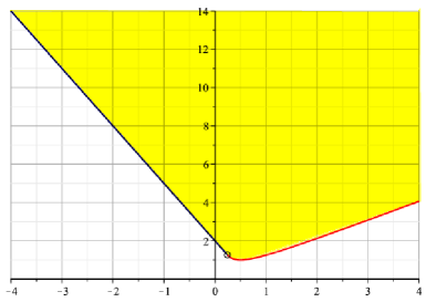
$A$

$\circ$

$B$

${\cal{P}}_{3}$

Figure 1: ${\cal{P}}_{3}$, $A=\big{(}\frac{2n-3}{4n},\frac{5}{4}\big{)}$, $B=\big{(}\frac{1}{2},1\big{)}$

Remark 9.

The expressions for $\kappa_{0}$ look complicated. A geometric visualization for the simplest cases will be helpful. Figure 1 depicts the case $n=3$. The yellow region is ${\cal{P}}$, the boundary of which is given by the curve $\kappa=\kappa_{0}(\lambda)$. The curve consists of a straight line (given by (3.1)), of slope $-n$, starting from $-\infty$, ending at the point $A$, and continues along a curvilinear path (in red, given by the equation $\kappa=\lambda+\frac{1}{4\lambda}$). The red curve attains a minimum at $B=\big{(}\frac{1}{2},1\big{)}$ ; see (3.3). If we extend the rectilinear boundary of $\cal P$ beyond $A$, it lies below the red curve, a fact manifested in (3.2). ∎

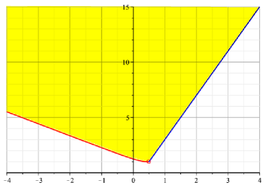
$A$

${\cal{P}}_{4}$

Figure 2: ${\cal{P}}_{4}$, $A=\big{(}\frac{1}{2},1\big{)}$

Figure 2 depicts the $n=4$ case. In contrast to the odd-order case, the rectilinear boundary of ${\cal{P}}$ starts from $A$ and points up towards $\lambda=\infty$; $A$ is the lowest point of ${\cal{P}}$. The red curvilinear path has a more complicated equation: $\textstyle\kappa=\frac{9\lambda^{2}+9\lambda+2\,\sqrt{(6\lambda^{2}-3\lambda+1)^{3}}-2}{27\lambda^{2}}\,.$

In the odd case, the point $A$ varies according to $n$, while in the even case, $A$ is fixed. The $y$-intercept of the boundary curve of ${\cal P}$ is $\frac{n+1}{2}$ for odd $n$, but is always $\frac{5}{4}$ for even $n$.

Proof. The existence of a smallest $\kappa_{0}$ for a given $\lambda$ follows from the convexity of ${\cal{P}}$.

By Lemma 1, $\textstyle\big{(}\frac{5}{4},\frac{2n-3}{4n}\big{)}\in{\cal P},$ $n$ odd. It is well-known that

$$\theta=n\sin(x)-\sin(nx)$$

is NN. Hence, for any $t>0$, $\phi+t\theta$ is NN and it corresponds to

$$\textstyle\big{(}nt+\frac{5}{4},\frac{2n-3}{4n}-t\big{)}\in{\cal P}.$$

These points are exactly the parametric representation of the straight line given by (3.1). We need to show they are actually boundary points.

It is easy to verify that both $\phi$ and $\theta$ satisfy (1.6). Hence $\phi+t\theta$ satisfies (1.6). Suppose we decrease the first coefficient $\kappa$. Then (1.4) is no longer satisfied and the polynomial is no longer NN. Thus, the corresponding $\kappa$ must be the smallest possible.

Similar arguments can be used to prove (3.5) for the even $n$ case, by using $\sigma$ of (1.1) which corresponds to $\big{(}1,\frac{1}{2}\big{)}\in{\cal P}$ (in place of $\phi$) and the NN polynomial $n\sin(x)+\sin(nx)$ to construct the rectilinear boundary of ${\cal P}$.

Next, we look at (3.2). Besides satisfying (1.6), $\phi$ satisfies (1.7) with equality, which is equivalent to the easily verified identity

$$1+4\,\sum_{k=1}^{2k}\,(-1)^{k+1}k^{3}+(4k-1)(2k+1)^{2}=0\,.$$ (3.6)

Let $\lambda>\frac{2n-3}{4n}$ and $\kappa=\frac{n+2}{2}-n\lambda$, then the polynomial corresponds to $\varphi=\phi-t\theta$ for some $t>0$. Since both $\phi$ and $\theta$ satisfy (1.6), so does $\varphi$. Now $\phi$ satisfies (1.7) with equality, but $-t\theta$ violates (1.7). Hence, $\varphi$ violates (1.7). By Proposition 3, $\theta$ cannot be NN.

To prove (3.3) and (3.4), we note that direct computation gives

$$\sigma(x)=\frac{c\big{(}\frac{1}{2}\big{)}}{2s\big{(}\frac{1}{2}\big{)}}\,(1-c_{n}).$$

This implies that $\sigma\big{(}\frac{2\pi}{n}\big{)}=\sigma^{\prime}\big{(}\frac{2\pi}{n}\big{)}=0$. For $\lambda>\frac{1}{2}$,

$$\eta=[1,1,\cdots,\lambda]_{s}=\sigma+\big{(}\lambda-\textstyle\frac{1}{2}\big{)}s_{n}.$$

It follows that $\eta\big{(}\frac{2\pi}{n}\big{)}=0$ and $\eta^{\prime}\big{(}\frac{2\pi}{n}\big{)}=\big{(}\lambda-\frac{1}{2}\big{)}c_{n}\big{(}\frac{2\pi}{n}\big{)}<0$. Consequently, $\eta(x)$ is negative in a right neighborhood of $x=\frac{2\pi}{n}$, and so $(1,\lambda)\not\in\cal P$.   

The equation of the curvilinear boundary of ${\cal P}_{3}$ is determined as follows. Since

$$\kappa\sin(x)+\sin(2x)+\lambda\sin(3x)=\sin(x)\left[4\lambda X^{2}+2X+(\kappa-\lambda)\right],$$

where $X=\cos(x)$, NN of the sine polynomial on the LHS is equivalent to the NN, in $[-1,1]$, of the algebraic polynomial in $X$ in square brackets on the RHS. It is obvious that the latter assertion is true if $\kappa$ is greater than or equal to

$$-\min_{\scriptscriptstyle X\in[-1,1]}\left\{4\lambda X^{2}+2X-\lambda\right\}$$

and the desired conclusion follows.

In theory, the same technique can be used to study the case of general $n$. The NN of $\phi$ is equivalent to that of an algebraic polynomial (determined using Chebyshev polynomials). Then $\kappa_{0}$ is the absolute value of the minimum value of this polynomial in $[-1,1]$. The determination of this value, however, becomes more difficult for large $n$.

The knowledge of ${\cal P}_{3}$ allows us to characterize all NN sine polynomials of degree 3 and all NN cosine polynomials of degree 2.

Corollary 1.

The sine polynomial $[a,b,c]_{s}$ is NN in $[0,\pi]$ iff

• $|b|\geq 4c$   and    $a-2|b|+3c\geq 0$, or

• $|b|<4c$   and    $a\geq c+\frac{b^{2}}{4c}$.

In all cases, a necessary condition is that $a\geq|b|$.

Proof. The case $b=0$ is trivial.

By making use of the reflection $x\mapsto-x$, we see that, without loss of generality, we may assume that $b>0$. The general case can be reduced to the case $b=1$ by dividing the sine polynomial by $b$ and then we are back to the ${\cal P}_{3}$ setting.   

Corollary 2.

The cosine polynomial $a+b\cos(2x)+c\cos(3x)$ is NN in $[0,\pi]$ iff

• $|b|\geq 4c$   and    $a-|b|+c\geq 0$, or

• $|b|<4c$   and    $a\geq c+\frac{b^{2}}{8c}$.

In all cases, a necessary condition is that $2a\geq|b|+c$.

Proof. The identity

$$a+b\cos(2x)+c\cos(3x)=\frac{(2a-c)\sin(x)+b\sin(2x)+c\sin(3x)}{2\sin(x)}$$

shows that the NN of the cosine polynomial in question is equivalent to the NN of the sine polynomial $[2a-c,b,c]_{s}$. The conclusions then follow from Corollary 1.

References

[1] H. Alzer, and M.K. Kwong,
Sturm theorem and a refinement of
Vietoris’ inequality for cosine polynomials,
(with H. Alzer),
arXiv:1406.0689 (math.CA).
[2]
A.S. Belov, Examples of trigonometric series with nonnegative partial sums, Math. USSR Sb. 186, 21¿46 (1995) (Russian); 186, 485¿510 (1995) (English translation).
[3] G. Brown,
Positivity and boundedness of trigonometric sums,
Analysis in Theory and Applications 23 (2007), 380-388.
[4] B. Dumitrescu, Positive Trigonometric Polynomials and Signal
Processing Applications, Springer, 2007.
[5] L. Fejér, Einige Sätze, die sich auf das Vorzeichen einer
ganzen rationalen Funktion beziehen, Monatsh. Math. Phys. 35 (1928),
305-344.
[6] S. Koumandos,
Inequalities for trigonometric sums, in: Nonlinear Analysis, Springer Optim. Appl. 68, P.M.
[7] M.K. Kwong,
An improved Vietoris sine inequalities,
J. Approx Theory, 189 (2015), 29-42.
[8] —,
Improved Vietoris Sine Inequalities for Non-Monotone, Non-Decaying Coefficients,
arXiv:1504.06705 [math.CA] (2015).