Computation of asymptotic expansions of turning point problems via Cauchy’s integral formula: Bessel functions

Abstract

Linear second order differential equations having a large real parameter and turning point in the complex plane are considered. Classical asymptotic expansions for solutions involve the Airy function and its derivative, along with two infinite series, the coefficients of which are usually difficult to compute. By considering the series as asymptotic expansions for two explicitly defined analytic functions, Cauchy’s integral formula is employed to compute the coefficient functions to high order of accuracy. The method employs a certain exponential form of Liouville-Green expansions for solutions of the differential equation, as well as for the Airy function. We illustrate the use of the method with the high accuracy computation of Airy-type expansions of Bessel functions of complex argument.

1 Introduction

In this paper we study linear second order differential equations having a simple turning point. Specifically, we consider the differential equation

$$d^{2}w/dz^{2}=\left\{{u^{2}f(z)+g(z)}\right\}w,$$ (1.1)

where $u$ is positive and large, $f(z)$ has a simple zero (turning point) at $z=z_{0}$ (say), and $f(z)$ and $g(z)$ are analytic in an unbounded domain containing the turning point.

This is a classical problem, with applications to numerous special functions. To obtain asymptotic solutions, the Liouville transformation

$$\frac{2}{3}\zeta^{3/2}=\pm\int_{z_{0}}^{z}f^{1/2}(t)dt,\quad W=\zeta^{-1/4}f^{1/4}(z)w,$$ (1.2)

is applied, where either sign in front of the integral can be chosen. As a result we transform (1.1) to the form

$$d^{2}W/d\zeta^{2}=\left\{u^{2}\zeta+\psi(\zeta)\right\}W,$$ (1.3)

where

$$\psi(\zeta)=\frac{5}{16\zeta^{2}}+\left\{4f(z){f}^{\prime\prime}(z)-5{f}^{\prime 2}(z)\right\}\frac{\zeta}{16f^{3}(z)}+\frac{\zeta g(z)}{f(z)}.$$ (1.4)

The lower integration limit in (1.2) ensures that the turning point $z=z_{0}$ of (1.1) is mapped to the turning point ${\zeta}=0$ of (1.3). Throughout this paper we shall assume that this turning point is bounded away from any other turning points or singularities of (1.1), equivalently $\psi(\zeta)$ is analytic for $0\leq\left|\zeta\right|<R$ for some positive $R$ which is independent of $u$.

When the turning point $z_{0}$ is real and $f(z)$ is real on a real interval around $z_{0}$, the sign in (1.2) is usually chosen in such a way that the new variable $\zeta$ is real when $z$ is real and in a neighborhood of the turning point.

From (Olver:1997:ASF, , Chap. 11, Theorem 9.1) we obtain solutions having the following asymptotic expansions in terms of Airy functions

$$\begin{array}[]{ll}W_{2n+1,j}(u,\zeta)=&\mathrm{Ai}_{j}\left(u^{2/3}\zeta\right)\displaystyle\sum_{s=0}^{n}\frac{\displaystyle{A_{s}(\zeta)}}{\displaystyle{u^{2s}}}\\ &+\frac{\displaystyle{\mathrm{Ai}_{j}^{\prime}\left(u^{2/3}\zeta\right)}}{\displaystyle{u^{4/3}}}\displaystyle\sum\limits_{s=0}^{n-1}{\frac{\displaystyle{B_{s}(\zeta)}}{\displaystyle{u^{2s}}}}+\varepsilon_{2n+1,j}(u,\zeta),\end{array}$$ (1.5)

for $j=0,\pm 1$. Here $\mathrm{Ai}_{j}(u^{2/3}\zeta)=\mathrm{Ai}(u^{2/3}\zeta e^{-2\pi ij/3})$, which are the Airy functions that are recessive in the sectors $\mathrm{\mathbf{S}}_{j}:=\left\{\zeta:|\mathrm{arg}(\zeta e^{-2\pi ij/3})|\leq\pi/3\right\}$ (Fig. 1); see (Olver:2010:AAR, , §9.2(iii)). Also, note that $\mathrm{Ai}_{j}^{\prime}(z)=d\mathrm{Ai}_{j}(z)/dz=e^{-2\pi ij/3}\mathrm{Ai}^{\prime}(ze^{-2\pi ij/3})$.

Figure 1: The sectors ${\rm\bf S}_{j}$ in the complex plane

From Olver’s explicit error bounds we have

$$\varepsilon_{2n+1,j}(u,\zeta)=\mathrm{env}\left\{\mathrm{Ai}_{j}\left(u^{2/3}\zeta\right)\right\}\mathcal{O}\left(u^{-2n-1}\right),$$

as $u\rightarrow\infty$, for $\zeta$ lying in certain domains described in (Olver:1997:ASF, , Chap. 11, §9), and which we assume to be unbounded. For a definition of the envelope function $\mathrm{env}$ for Airy functions, see (Olver:2010:AAR, , §2.8(iii)).

In (1.5) $A_{0}(\zeta)$ is an arbitrary non-zero constant (typically taken to be 1), and for $s=0,1,2,\cdots$, the other coefficients satisfy the recursion relations

$$B_{s}(\zeta)=\frac{1}{2\zeta^{1/2}}\int_{0}^{\zeta}\left\{\psi(t)A_{s}(t)-A_{s}^{\prime\prime}(t)\right\}\frac{dt}{t^{1/2}},$$ (1.6)

and

$$A_{s+1}(\zeta)=-\frac{1}{2}B_{s}^{\prime}(\zeta)+\frac{1}{2}\int\psi(\zeta)B_{s}(\zeta)d\zeta.$$ (1.7)

We remark that the lower integration limit in (1.6) must be $0$ in order for each $B_{s}(\zeta)$ to be analytic at $\zeta=0$, whereas in (1.7) there is no restriction in the choice of integration constant. This will be of significance to us below.

In general, these coefficients are difficult to compute, primarily due to the requirement of repeated integrations. They also show cancellations near the turning point. For complex $\zeta$ close to $0$ one can compute these coefficients in a numerically stable way by considering power series expansions for the coefficients, as done in Amos:1986:A6A ; Amos:1977:C6S , where they are expanded in powers of $\omega=\sqrt{1-z^{2}}$. For other computational approaches to compute the coefficients, and in particular for real values of $\zeta$, see Temme:1997:NAF .

The purpose of this paper is to provide a more simple means of computing a large number of these terms. We shall employ Cauchy’s integral formula to do so, and our results will be valid for real and complex $\zeta$ lying in a bounded (but not necessarily small) domain containing the turning point $\zeta=0$. Our approach can potentially be extended to other situations, including the cases of simple poles (Olver:1997:ASF, , Chap. 12), and coalescing turning points.

We illustrate the use of the method with the high accuracy computation of Airy-type expansions of Bessel functions of complex argument.

2 General method

We first present Liouville-Green expansions for solutions of (1.1), a certain form of which will be required for our method. These only involve elementary (exponential) functions, but are not valid at the turning point. The appropriate Liouville-Green transformation is given by (Olver:1997:ASF, , Chap. 10, §2), namely

$$\xi=\frac{2}{3}\zeta^{3/2},\ V=f^{1/4}(z)w.$$ (2.1)

With these, equation (1.1) is transformed to equation

$$d^{2}V/d\xi^{2}=\left\{u^{2}+\phi(\xi)\right\}V,$$ (2.2)

where

$$\phi(\xi)=\frac{4f(z)f^{\prime\prime}(z)-5f^{\prime 2}(z)}{16f^{3}(z)}+\frac{g(z)}{f(z)}.$$ (2.3)

The branch for the first of (2.1) will be dependent on the solutions under consideration, as described below. Note, as $\zeta$ completes one circuit about the turning point $\zeta=0$, the variable $\xi$ correspondingly crosses more than one Riemann sheet.

It turns out that solutions where asymptotic expansions appear inside exponentials are more convenient for our purposes. Specifically, from (Olver:1997:ASF, , Chap. 10, Ex. 2.1) we have solutions

$$V_{n}^{\pm}(u,\xi)=\exp\left\{\pm u\xi+\displaystyle\sum_{s=1}^{n-1}(\pm 1)^{s}\frac{E_{s}(\xi)}{u^{s}}\right\}+\varepsilon_{n}^{\pm}(u,\xi).$$ (2.4)

In these, the coefficients are given by

$$E_{s}(\xi)=\int F_{s}(\xi)d\xi\quad(s=1,2,3,\cdots),$$ (2.5)

where

$$F_{1}(\xi)=\frac{1}{2}\phi(\xi),\quad F_{2}(\xi)=-\frac{1}{4}\phi^{\prime}(\xi),$$ (2.6)

and

$$F_{s+1}(\xi)=-\frac{1}{2}F_{s}^{\prime}(\xi)-\frac{1}{2}\displaystyle\sum_{j=1}^{s-1}F_{j}(\xi)F_{s-j}(\xi)\quad(s=2,3,\cdots).$$ (2.7)

Primes are derivatives with respect to $\xi$. The integration constants in (2.5) will be discussed below, and we find that for the odd coefficients $E_{2j+1}(\xi)$ ($j=0,1,2,\cdots$) they must be suitably chosen.

Explicit error bounds for $\varepsilon_{n}^{\pm}(u,\xi)$, which verify the asymptotic validity of the expansions (2.4), are given in Dunster:1998:AOT . In particular, for arbitrary $\delta>0$, under certain conditions on $\psi(\xi)$, we have that $\varepsilon_{n}^{\pm}(u,\xi)=e^{\pm u\xi}\mathcal{O}\left(u^{-n}\right)$ as $\xi\rightarrow\infty$ in certain domains $\Xi^{\pm}$ as described in (Olver:1997:ASF, , Chap. 10, §3). These are the same as those for the corresponding asymptotic solutions of the more common form

$$V\sim\exp\{\pm u\xi\}\sum_{s=0}^{\infty}(\pm 1)^{s}A_{s}(\xi)u^{-s}.$$ (2.8)

It is the relation (2.7) that is the reason why the expansions (2.4) are numerically advantageous: the coefficients $F_{s}(\xi)$ can all be determined explicitly without resorting to integration. Furthermore, from (2.5) we observe that only one integration is required (numerical or explicit) to evaluate each $E_{s}(\xi)$, as opposed to repeated integrals for computing the coefficients $A_{s}(\xi)$ in (2.8).

Remarkably, it turns out that integration is not required to evaluate the even terms $E_{2j}(\xi)$ ($j=1,2,3,\cdots$). To see this, consider the Wronskian of the solutions $V_{n}^{\pm}(u,\xi)$ given by (2.4). Since this is a constant (by Abel’s theorem) we infer that

$$\left\{u+\sum_{j=0}^{\infty}\frac{F_{2j+1}(\xi)}{u^{2j+1}}\right\}\exp\left\{2\sum_{j=1}^{\infty}\frac{E_{2j}(\xi)}{u^{2j}}\right\}\sim\mbox{constant,}$$

which, on taking logarithms, yields

$$\sum_{j=1}^{\infty}\frac{E_{2j}(\xi)}{u^{2j}}\sim-\frac{1}{2}\ln\left\{1+\sum_{j=0}^{\infty}\frac{F_{2j+1}(\xi)}{u^{2j+2}}\right\}+\mbox{constant.}$$ (2.9)

We then asymptotically expand the RHS of this relation in inverse powers of $u^{2}$, and equate the coefficients of both sides. As a result, we find that (to within an arbitrary additive constant in each instance)

$$E_{2}(\xi)=-\frac{1}{2}F_{1}(\xi),\,E_{4}(\xi)=\frac{1}{4}F_{1}^{2}(\xi)-\frac{1}{2}F_{3}(\xi),$$ (2.10)

and so on. In particular, the even coefficients $E_{2j}(\xi)$ ($j=1,2,3,\cdots$) are explicitly given in terms of $F_{2k+1}(\xi)$ ($k=0,1,2,\cdots,j-1$) (which in turn are given by (2.6) and (2.7)).

At this stage we consider Liouville-Green solutions of (1.3). Comparing (1.2), (2.1) and (2.4) we obtain three asymptotic solutions $W_{j}(u,\zeta)$ ($j=0,\pm 1$) of (1.3) which are recessive (respectively) for $\zeta\in\mathrm{\mathbf{S}}_{j}$, possessing the asymptotic expansions

$$W_{0}(u,\zeta)\sim{\zeta^{-1/4}}\exp\left\{-\frac{2}{3}u\zeta^{3/2}+\displaystyle\sum_{s=1}^{\infty}(-1)^{s}\frac{E_{s}(\xi)}{u^{s}}\right\},$$ (2.11)

and

$$W_{j}(u,\zeta)\sim{\zeta^{-1/4}}\exp\left\{\frac{2}{3}u\zeta^{3/2}+\displaystyle\sum_{s=1}^{\infty}\frac{E_{s}(\xi)}{u^{s}}\right\}\ (j=\pm 1),$$ (2.12)

as $u\rightarrow\infty,$ uniformly for $\zeta\in\Omega_{j}$ (say). For $j=0,\pm 1$ the branches are such that ${\rm Re}\left(e^{-ij\pi}\zeta^{3/2}\right)\geq 0$ for $\zeta\in\mathrm{\mathbf{S}}_{j}$ , and ${\rm Re}\left(e^{-ij\pi}\zeta^{3/2}\right)\leq 0$ for $\zeta\notin\mathrm{\mathbf{S}}_{j}$. As is typically the case in practice, for each $j$ we assume that $\Omega_{j}\cap\mathrm{\mathbf{S}}_{j}$ is unbounded.

We remark that, on account of the analyticity of $\psi(\zeta)$ in the disk $0\leq\left|\zeta\right|<R$, the expansions (2.11) and (2.12) certainly hold in the bounded sector $\delta\leq\left|\zeta\right|<R$, $|\mathrm{arg}(\zeta e^{-2\pi ij/3})|\leq\pi-\delta$, where here and elsewhere $\delta$ denotes an arbitrary small positive constant. We also note that the recessive property at $\zeta=\infty$ in $\Omega_{j}\cap\mathrm{\mathbf{S}}_{j}$ uniquely defines $W_{j}(u,\zeta)$ up to a multiplicative constant. Indeed, we have that $W_{j}(u,\zeta)=c_{2n+1,j}W_{2n+1,j}(u,\zeta)$ for some constants $c_{2n+1,j}$, although we shall not use these relations.

Now, since no two from these three solutions are linearly dependent, we can assume they satisfy a connection formula of the form

$$\lambda_{-1}W_{-1}(u,\zeta)=iW_{0}(u,\zeta)+\lambda_{1}W_{1}(u,\zeta),$$ (2.13)

for certain constants $\lambda_{-1}$ and $\lambda_{1}$ (which may of course depend on $u$). The factor $i$ is for convenience.

We note that each $W_{j}(u,\zeta)$ ($j=0,\pm 1$), being a solution of (1.1), is analytic in a neighborhood of the turning point. Based on (1.5), and following Boyd:1987:AEF ; Temme:1997:NAF , we thus can define functions $A(u,z)$ and $B(u,z)$, analytic at $z=z_{0}$ ($\zeta=0$), implicitly by the pair of equations

$$\frac{\displaystyle{1}}{\displaystyle{2\pi^{1/2}u^{1/6}}}W_{0}(u,\zeta)=\mathrm{Ai}_{0}(u^{2/3}\zeta)A(u,z)+\mathrm{Ai}_{0}^{\prime}(u^{2/3}\zeta)B(u,z),$$ (2.14)

and

$$\frac{e^{\pi i/6}\lambda_{1}}{2\pi^{1/2}u^{1/6}}W_{1}(u,\zeta)=\mathrm{Ai}_{1}(u^{2/3}\zeta)A(u,z)+\mathrm{Ai}_{1}^{\prime}(u^{2/3}\zeta)B(u,z),$$ (2.15)

where (as shown below) the multiplicative constants on the LHS of both equations have been chosen to yield the appropriate behavior of $A(u,z)$ and $B(u,z)$ as $u\rightarrow\infty$. We remark that for computational purposes it is more convenient to consider $A(u,z)$ and $B(u,z)$ as functions of $z$, although in deriving their asymptotic expansions we shall regard them as functions of $\zeta$ as necessary.

Next, from the connection formula (2.13), and the corresponding well-known connection formula for the Airy functions

$$\mathrm{Ai}_{-1}\left(u^{2/3}\zeta\right)=e^{-\pi i/3}\mathrm{Ai}_{1}\left(u^{2/3}\zeta\right)+e^{\pi i/3}\mathrm{Ai}_{0}\left(u^{2/3}\zeta\right),$$

we derive from (2.14) and (2.15) the following Airy function representation for the solution which is recessive in $\mathrm{\mathbf{S}}_{-1}$

$$\frac{\displaystyle{e^{-\pi i/6}\lambda_{-1}}}{\displaystyle{2\pi^{1/2}u^{1/6}}}W_{-1}(u,\zeta)=\mathrm{Ai}_{-1}(u^{2/3}\zeta)A(u,z)+\mathrm{Ai}_{-1}^{\prime}(u^{2/3}\zeta)B(u,z).$$ (2.16)

We shall show, using (2.14), (2.15) and (2.16), that $A(u,z)$ and $B(u,z)$ are slowly varying relative to the fast variation of the Airy functions in a full neighborhood of turning point. Specifically, on referring to (1.5), $A(u,z)$ and $B(u,z)$ will admit the following asymptotic expansions as $u\rightarrow\infty$

$$A(u,z)\sim\displaystyle\sum_{s=0}^{\infty}\frac{A_{s}(\zeta)}{u^{2s}},\,B(u,z)\sim\frac{1}{u^{4/3}}\displaystyle\sum_{s=0}^{\infty}\frac{B_{s}(\zeta)}{u^{2s}},$$ (2.17)

uniformly with respect to $\zeta$ lying in a certain unbounded domain which contains the disk $0\leq\left|\zeta\right|<R$.

To show the slowly-varying nature of $A(u,z)$ and $B(u,z)$ (for example) when $\zeta\in\left\{\mathrm{\mathbf{S}}_{0}\cap\Omega_{0}\right\}\cup\left\{\mathrm{\mathbf{S}}_{-1}\cap\Omega_{-1}\right\}$, we solve (2.14) and (2.16) for the coefficients, and using the Wronskian for Airy functions (Olver:2010:AAR, , §9.2(iv)), we arrive at the explicit representations

$$\begin{array}[]{ll}A(u,z)=\frac{\displaystyle{\pi^{1/2}}}{\displaystyle{u^{1/6}}}&\left\{e^{\pi i/6}W_{0}(u,\zeta)\mathrm{Ai}_{-1}^{\prime}(u^{2/3}\zeta)\right.\\ &\left.-\lambda_{-1}W_{-1}(u,\zeta)\mathrm{Ai}_{0}^{\prime}(u^{2/3}\zeta)\right\},\end{array}$$ (2.18)

and

$$\begin{array}[]{ll}B(u,z)=\frac{\displaystyle{\pi^{1/2}}}{\displaystyle{u^{1/6}}}&\left\{\lambda_{-1}W_{-1}(u,\zeta)\mathrm{Ai}_{0}(u^{2/3}\zeta)\right.\\ &\left.-e^{\pi i/6}W_{0}(u,\zeta)\mathrm{Ai}_{-1}(u^{2/3}\zeta)\right\}.\end{array}$$ (2.19)

Then for $\zeta\in\left\{\mathrm{\mathbf{S}}_{0}\cap\Omega_{0}\right\}\cup\left\{\mathrm{\mathbf{S}}_{-1}\cap\Omega_{-1}\right\}$ each product pair of functions on the RHS of (2.18) and (2.19) consists of one exponentially small function times an exponentially large one. Consequently these forms are numerically satisfactory in that domain.

At this stage the integration constants in (2.5) are arbitrary, and indeed do not have to be independent of $u$. Therefore, for notational convenience, in (2.18) and (2.19) we shall absorb the coefficient $\lambda_{-1}$ into the expansion (2.12) for $W_{-1}(u,\zeta)$, by redefining the Liouville-Green coefficients if necessary. For example,we can redefine $E_{1}(\xi)$ to be $E_{1}(\xi)-\frac{1}{2}u\ln\left(\lambda_{-1}\right)$ and $E_{2}(\xi)$ to be $E_{2}(\xi)-\frac{1}{2}u^{2}\ln\left(\lambda_{-1}\right)$: as a result $\lambda_{-1}W_{-1}(u,\zeta)$ is scaled to become $W_{-1}(u,\zeta)$, whereas from (2.11) we see that $W_{0}(u,\zeta)$ is unchanged.

We now use (A.3) and (A.4), along with the corresponding expansions (which are valid for $\left|{\arg\left({\zeta e^{2\pi i/3}}\right)}\right|\leq\pi-\delta$)

$$\mathrm{Ai}_{-1}\left(u^{2/3}\zeta\right)\sim\frac{e^{-\pi i/6}}{2\pi^{1/2}u^{1/6}\zeta^{1/4}}\exp\left\{u\xi+\sum\limits_{s=1}^{\infty}\frac{a_{s}}{su^{s}\xi^{s}}\right\},$$

and

$$\mathrm{Ai}_{-1}^{\prime}\left(u^{2/3}\zeta\right)\sim\frac{e^{-\pi i/6}u^{1/6}\zeta^{1/4}}{2\pi^{1/2}}\exp\left\{u\xi+\sum\limits_{s=1}^{\infty}\frac{\tilde{{a}}_{s}}{su^{s}\xi^{s}}\right\}.$$

Then, from (2.18) and (2.19), along with the defining expansions (2.4), we obtain our main result, the slowly-varying expansions

$$\begin{array}[]{ll}A(u,z)\sim&\exp\left\{\displaystyle\sum_{j=1}^{\infty}\frac{\displaystyle{E_{2j}(\xi)+\tilde{a}_{2j}\xi^{-2j}/(2j)}}{\displaystyle{u^{2j}}}\right\}\\ &\times\mathrm{cosh}\left\{\displaystyle\sum_{j=0}^{\infty}\frac{\displaystyle{E_{2j+1}(\xi)-\tilde{a}_{2j+1}\xi^{-2j-1}/(2j+1)}}{\displaystyle{u^{2j+1}}}\right\},\end{array}$$ (2.20)

and

$$\begin{array}[]{ll}B(u,z)\sim&\frac{\displaystyle{1}}{\displaystyle{u^{1/3}\zeta^{1/2}}}\exp\left\{\displaystyle\sum_{j=1}^{\infty}\frac{\displaystyle{E_{2j}(\xi)+a_{2j}\xi^{-2j}/(2j)}}{\displaystyle{u^{2j}}}\right\}\\ &\times\mathrm{sinh}\left\{\displaystyle\sum_{j=0}^{\infty}\frac{\displaystyle{E_{2j+1}(\xi)-a_{2j+1}\xi^{-2j-1}/(2j+1)}}{\displaystyle{u^{2j+1}}}\right\}.\end{array}$$ (2.21)

These asymptotic expansions certainly hold for (at least) $-\pi+\delta\leq\mathrm{arg}(\zeta)\leq\frac{1}{3}\pi-\delta,$ $0<\left|\zeta\right|<R$. Similar slowing-varying expansions can be obtained for all other values of $\mathrm{arg}(\zeta)$ near the turning point, by solving for $A(u,z)$ and $B(u,z)$ from a suitably chosen pair from the three equations (2.14), (2.15) and (2.16). Each of these expansions can be expressed in the same form as above, except that the coefficients $E_{s}(\xi)$ may differ by the integration constants in (2.5).

In fact, if these integration constants are arbitrarily chosen, we find that the RHS of (2.20) and (2.21) generally each has a branch point at $\zeta=0$ ($z=z_{0}$). Hence, being multi-valued (in fact unbounded) for small $\zeta$, the expansions are generally only valid for restricted $\arg(\zeta)$ near the turning point. It is only for specific integration constants in (2.5), at least for the odd coefficients $E_{2j+1}(\xi)$ ($j=0,1,2\cdots$), that the expansions are single-valued, and hence by a continuity argument (2.20) and (2.21) hold for $0<\left|\zeta\right|<R$, with $\mathrm{arg}(\zeta)$ unrestricted. This essentially corresponds to the choice of the lower integration constant in (1.6), which (as remarked above) ensures that each coefficient $B_{s}(\zeta)$ is analytic at $\zeta=0$.

Recalling that $\xi=\frac{2}{3}\zeta^{3/2}$, it is straightforward to show that the expansions (2.20) and (2.21) are single-valued at $\zeta=0$ if $\zeta^{1/2}E_{2j+1}(\xi)$ and $E_{2j}(\xi)$ ($j=0,1,2,\cdots$) are meromorphic: here and throughout meromorphic means with respect to $\zeta$, and at $\zeta=0$. If we assume for the moment that this is true for $\zeta^{1/2}E_{2j+1}(\xi)$ and $E_{2j}(\xi)$, then on re-expanding (2.20) and (2.21) into the forms (2.17), we deduce that the coefficients $A_{s}(\zeta)$ and $B_{s}(\zeta)$ in the latter expansions must be single-valued. By a uniqueness argument these coefficients must satisfy (1.6) and (1.7), and moreover single-valuedness means the lower integration limit in the former must indeed be 0. But in this case we know that $A_{s}(\zeta)$ and $B_{s}(\zeta)$ are actually analytic at $\zeta=0$. We deduce that if $\zeta^{1/2}E_{2j+1}(\xi)$ and $E_{2j}(\xi)$ are meromorphic then (2.20) and (2.21) have a removable singularity when they are re-expanded into the forms (2.17). With an appropriate choice of integration constant for each $E_{2j+1}(\xi)$ ($j=0,1,2,\cdots$) we now show that this is indeed so.

To this end, we first note from (1.4) and (2.3) that

$$\phi(\xi)=\frac{\psi(\zeta)}{\zeta}-\frac{5}{16\zeta^{3}},$$ (2.22)

and hence this function is meromorphic. Therefore, on noting that $d\xi/d\zeta=\zeta^{1/2}$, we find by induction from (2.5) - (2.7) that $\zeta^{1/2}F_{2j}(\xi)$ and $F_{2j+1}(\xi)$ are also meromorphic.

To establish the desired meromorphicity of $\zeta^{1/2}E_{2j+1}(\xi)$ and $E_{2j}(\xi)$, let us consider these separately. Firstly, from (2.5) we see that $\zeta^{1/2}{E_{2j+1}(\xi)}$ is meromorphic if and only if the Laurent-type expansion

$$\zeta^{1/2}E_{2j+1}(\xi)=\zeta^{1/2}\int\zeta^{1/2}F_{2j+1}(\xi(\zeta))d\zeta=\alpha_{2j+1}\zeta^{1/2}+\sum_{k=-2j-1}^{\infty}\alpha_{2j+1,k}\zeta^{k},$$ (2.23)

satisfies $\alpha_{2j+1}=0$. Clearly the integration constants in (2.5) can be selected in order for this to be so, and we assume this from now on.

Next consider the even terms. Again from (2.5), we observe that

$$E_{2j}(\xi)=\int\zeta^{1/2}F_{2j}(\xi(\zeta))d\zeta,$$ (2.24)

must either be meromorphic, or have a logarithmic singularity at $\zeta=0$. However, the latter possibility can immediately be discarded by referring to (2.9) along with the meromorphicity of $F_{2j+1}(\xi)$. We note that the integration constants in (2.24) do not affect the meromorphicity of $E_{2j}(\xi)$, and hence they can be arbitrarily chosen.

In summary, we have established that $\alpha_{2j+1}=0$ in (2.23) is a necessary and sufficient condition for the expansions (2.20) and (2.21) to be valid in a neighborhood of the turning point with $\mathrm{arg}(\zeta)$ unrestricted.

In practice there are several ways of ensuring the correct choice of $E_{2j+1}(\xi)$. If each of these functions can be explicitly determined from (2.5), then a symbolic algebra system could be used to determine the expansion (2.23), and if $\alpha_{2j+1}\neq 0$ one can simply subtract this constant from the function given by the anti-derivative derived from (2.5).

If explicit integration of (2.5) is not possible, and quadrature is required, then from (2.23) we observe that

$$\alpha_{2j+1}=\frac{1}{2}\left\{E_{2j+1}(\xi^{\ast})+E_{2j+1}(\xi)\right\},$$ (2.25)

where $\xi^{\ast}=\xi(\zeta e^{2\pi i})$. Since the coefficients will be computed numerically on a loop surrounding $\zeta=0$, the values on the RHS of (2.25) can also be computed, provided $\xi$ and $\xi^{\ast}$ correspond to the initial and terminal points of the loop. Hence, as in the case of the explicitly known coefficients, these numerically computed values can be subtracted from the initial values of $E_{2j+1}(\xi)$ evaluated from (2.5).

In the common situation where $\psi(\zeta)$ is real in some real interval $(-a,a)$ where $a>0$, this numerical method can be simplified somewhat. Specifically, if we choose the lower limit of integration in (2.5) to be at a real point on our path of integration, $\xi=\xi(\zeta_{0})$ say, where $0<\zeta_{0}<a$, then we similarly find from (2.23) that

$$\alpha_{2j+1}=\mathrm{Re}\left\{E_{2j+1}\left(\xi(\zeta_{0}e^{\pi i})\right)\right\},$$ (2.26)

and we can then proceed as above.

We summarize the principal result as follows.

Theorem 2.1

For the differential equation

$$d^{2}w/dz^{2}=\left\{{u^{2}f(z)+g(z)}\right\}w,$$ (2.27)

assume $u$ is positive and large, $f(z)$ has a simple zero at $z=z_{0}$, and $f(z)$ and $g(z)$ are analytic in a domain $D$ containing $z_{0}$. Further assume that $f(z)$ does not vanish in the disk $D\left(z_{0},\rho\right):=\left\{z:0<\left|z-z_{0}\right|<\rho\right\}\subset D$. Define variables $\xi$ and $\zeta$ by

$$\xi=\frac{2}{3}\zeta^{3/2}=\int_{z_{0}}^{z}f^{1/2}(t)dt,$$ (2.28)

and let $\mathrm{Ai}_{j}(u^{2/3}\zeta)$ ($j=0,\pm 1$) denote the Airy functions $\mathrm{Ai}(u^{2/3}\zeta e^{-2\pi ij/3})$. Then there exist three numerically satisfactory solutions of (2.27) given by

$$w_{j}\left(u,z\right)=\zeta^{1/4}f^{-1/4}(z)\left\{\mathrm{Ai}_{j}(u^{2/3}\zeta)A(u,z)+\mathrm{Ai}_{j}^{\prime}(u^{2/3}\zeta)B(u,z)\right\}.$$ (2.29)

In these, the coefficient functions $A(u,z)$ and $B(u,z)$ are analytic at $z=z_{0}$, and possess the asymptotic expansions (2.20) and (2.21) in a domain that includes $D\left(z_{0},\rho\right)$. Here $a_{1}=a_{2}=\frac{5}{72}$, $\tilde{a}_{1}=\tilde{a}_{2}=-\frac{7}{72}$, and in both cases subsequent terms are given by (A.2). The coefficients $E_{s}(\xi)$ ($s=1,2,3,\cdots$) are given by (2.5) - (2.7), where the integration constants for the odd coefficients in (2.5) must be selected so that $\zeta^{1/2}E_{2j+1}(\xi)$ ($j=0,1,2,\cdots$) is meromorphic as a function of $\zeta$ at $\zeta=0$; i.e. $\zeta^{1/2}E_{2j+1}(\xi)$ possesses the Laurent expansion (2.23) with $\alpha_{2j+1}=0$.

Remark 2.1

The even terms $E_{2j}(\xi)$ ($j=1,2,3,\cdots$) can alternatively be evaluated by expanding the RHS of (2.9) in inverse powers of $u^{2}$, and equating the coefficients of both sides. This avoids integration for evaluating these terms. We also note that the expansions (2.20) and (2.21) are valid in the same domains as those for the corresponding asymptotic solutions of (Olver:1997:ASF, , Chap. 11, Theorem 9.1), and can be unbounded provided $f(z)$ and $g(z)$ have the appropriate behavior at $\infty$ (see (Olver:1997:ASF, , Chap. 11, Sect. 9.3)).

Our focus is to utilize the expansions (2.20) and (2.21) to efficiently compute $A(u,z)$ and $u^{4/3}B(u,z)$ to $\mathcal{O}\left(u^{-2m}\right)$ for some prescribed $m$. As we shall see in the application to Bessel functions below, in general it may be more convenient to consider scaled functions

$$\mathcal{A}(u,z)=\phi(u,z)A(u,z),\,\mathcal{B}(u,z)=\phi(u,z)B(u,z),$$ (2.30)

where $\phi(u,z)$ is some suitably chosen function which is analytic in a domain $\Omega$ (say) in which the expansion (2.20) is valid.

Our aim is to employ the Cauchy integrals

$$\mathcal{A}(u,z)=\frac{1}{2\pi i}\oint\limits_{\mathcal{L}}\frac{\phi(u,t)A(u,t)}{t-z}dt,\,\mathcal{B}(u,z)=\frac{1}{2\pi i}\oint\limits_{\mathcal{L}}\frac{\phi(u,t)B(u,t)}{t-z}dt,$$ (2.31)

where $\mathcal{L}$ is a positively orientated closed loop lying in $\Omega$ and surrounding $t=z$ and $t=z_{0}$, and therefore (2.20) and (2.21) can be inserted in the respective integrands. As we showed above, the asymptotic expansions (2.20) and (2.21) are in theory valid close to the turning point $\xi=\zeta=0$ ($z=z_{0}$) as $u\rightarrow\infty$. However, for fixed $u$ the terms in the series become unbounded as $\xi\rightarrow 0$, and therefore these series are numerically unsatisfactory near the turning point. It is for this reason that we use the Cauchy integral formulas (2.31) for their numerical approximation.

At this point, it is important to realize that we will needed to compute the coefficients $E_{s}(\xi)$ in (2.20) and (2.21) at specific fixed points on $\mathcal{L}$. Since this computation is done once and for all the computational efficiency in the computation of these coefficients is not so important. And, as noted earlier, if the integrals in (2.5) cannot be explicitly evaluated, only one numerical evaluation of an integral is required for each odd coefficient.

For our purposes it will be sufficient to consider a circular path of integration with center at $z_{c}$, not necessarily with $z_{c}=z_{0}$, but which in any case must contain the turning point $z_{0}$. For computing the integral, we therefore use the parametrization $t(\theta)=z_{c}+Re^{i\theta}$, $\theta\in[0,2\pi]$ and we have

$$\mathcal{A}(u,z)=\frac{1}{2\pi}\int_{0}^{2\pi}F(\theta)d\theta,\,F(\theta)=\mathcal{A}(u,t(\theta))\frac{t(\theta)-z_{c}}{t(\theta)-z},$$ (2.32)

and likewise for $\mathcal{B}(u,z)$. The function $F(\theta)$ is periodic and we are integrating over one period. Since the function is infinitely differentiable as a function of $\theta$ we can expect that the trapezoidal rule will give good convergence (Gil:2007:NSF, , Thm. 5.6). We write $\theta_{j}=2\pi j/N$ ( $j=0,1,\dots N$) and we have

$$\int_{0}^{2\pi}F(\theta)d\theta\approx\frac{2\pi}{N}\left\{\frac{1}{2}(F(\theta_{0})+F(\theta_{N}))+\sum_{j=1}^{N-1}F(\theta_{j})\right\},$$

and therefore

$$\mathcal{A}(u,z)\approx\frac{1}{N}\sum_{j=1}^{N}F(2\pi j/N).$$ (2.33)

Numerical experiments show that $N$ does not need to be large and that, for instance in our application to Bessel equation (see §5.2), $N=500$ is enough for more than $15$-digits accuracy in a wide region around the turning point (namely for $z_{c}=2$, $R=1.8$); the number can be reduced for smaller regions, and for $z_{c}=1$, $R=0.5$, $15$ digits accuracy is reached with $N=150$. This is consistent with the expected good performance of the trapezoidal rule.

For the derivatives of solutions $w_{j}(u,z)$ (say) of (1.1), suppose scaled coefficient functions $\mathcal{A}(u,z)$ and $\mathcal{B}(u,z)$ are defined by

$$\lambda_{j}w_{j}(u,z)=\mathrm{Ai}_{j}\left(u^{2/3}\zeta\right)\mathcal{A}(u,z)+\mathrm{Ai}_{j}^{\prime}\left(u^{2/3}\zeta\right)\mathcal{B}(u,z)\ (j=\pm 1),$$ (2.34)

for some appropriate connection coefficients $\lambda_{\pm 1}$. We can then proceed similarly as before, by defining corresponding coefficients $\mathcal{C}(u,z)$ and $\mathcal{D}(u,z)$ by

$$\lambda_{j}w_{j}^{\prime}(u,z)=\mathrm{Ai}_{j}\left(u^{2/3}\zeta\right)\mathcal{C}(u,z)+\mathrm{Ai}_{j}^{\prime}\left(u^{2/3}\zeta\right)\mathcal{D}(u,z)\ (j=\pm 1).$$ (2.35)

Then, solving for these coefficients, we obtain the same expressions as for the previous coefficients, but with $w_{j}\left({u,z}\right)$ substituted by their derivatives. Then, to obtain similar expansions to (2.20) and (2.21), we would also need the Liouville-Green expansions for the derivatives of these functions, which can be obtained by differentiation of the corresponding expansions for the functions themselves.

A preferable way to compute the new coefficients is to differentiate (2.34). After differentiating with respect to $z$, using the Airy differential equation to eliminate the second derivative of the Airy functions, then solving and comparing to (2.35), we obtain the relations

$$\mathcal{C}(u,z)={\mathcal{A}}^{\prime}(u,z)+u^{4/3}\zeta(z)\zeta^{\prime}(z)\mathcal{B}(u,z),$$ (2.36)

and

$$\mathcal{D}(u,z)=u^{2/3}\zeta^{\prime}(z)\mathcal{A}(u,z)+{\mathcal{B}}^{\prime}(u,z).$$ (2.37)

To compute the derivatives of the coefficients we can also use Cauchy’s integral formula to write

$$\mathcal{A}^{\prime}(u,z)=\frac{1}{2\pi i}\oint\limits_{\mathcal{L}}\frac{\mathcal{A}(u,t)}{(t-z)^{2}}dt,\ \mathcal{B}^{\prime}(u,z)=\frac{1}{2\pi i}\oint\limits_{\mathcal{L}}\frac{\mathcal{B}(u,t)}{(t-z)^{2}}dt.$$ (2.38)

Then, from (2.30), (2.31), and (2.36) - (2.38) we obtain

$$\mathcal{C}(u,z)=\frac{1}{2\pi i}\oint\limits_{\mathcal{L}}\frac{\mathcal{A}(u,t)+u^{4/3}{(t-z)}\zeta(t)\zeta^{\prime}(t)\mathcal{B}(u,t)}{(t-z)^{2}}dt,$$ (2.39)

and

$$\mathcal{D}(u,z)=\frac{{1}}{{2\pi i}}\oint\limits_{\mathcal{L}}\frac{\mathcal{B}(u,t)+u^{2/3}{(t-z)}\zeta^{\prime}(t)\mathcal{A}(u,t)}{{(t-z)^{2}}}dt.$$ (2.40)

We then use the computed values of $\mathcal{A}(u,t)$ and $\mathcal{B}(u,t)$ on $\mathcal{L}$, and proceed as above. Again, the trapezoidal rule is a good choice; in fact, it is in some sense optimal Bornemann:2011:AAS .

We remark that it is desirable that (2.36) and (2.37) be numerically stable, in the sense that, for large $u$, there is no cancellation in leading order terms in the two terms in either representation. The choice of scaling function $\phi(u,z)$ in (2.30) should be such that this is indeed the case.

3 Bessel’s equation: preliminary transformations

We illustrate the new technique using the Airy function asymptotic expansions for Bessel functions. The first step in doing so, is to apply the Liouville transformations described in §§1 and 2 to Bessel’s equation. To this end, we first note that functions $w=z^{1/2}J_{\nu}(\nu z)$, $w=z^{1/2}H_{\nu}^{(1)}(\nu z)$ and $w=z^{1/2}H_{\nu}^{(2)}(\nu z)$ satisfy

$$\frac{d^{2}w}{dz^{2}}=\left\{\nu^{2}\frac{1-z^{2}}{z^{2}}-\frac{1}{4z^{2}}\right\}w.$$

Here $\nu$ plays the role of our large positive parameter $u$, and $z$ is complex.

From (1.2), and taking the negative sign, let

$$\frac{2}{3}\zeta^{3/2}=\ln\left\{\frac{1+\left({1-z^{2}}\right)^{1/2}}{z}\right\}-\left({1-z^{2}}\right)^{1/2},$$ (3.1)

and

$$W=\zeta^{-1/4}\left(\frac{1-z^{2}}{z^{2}}\right)^{1/4}w.$$

The transformed variable $\zeta$ is real for real $z\in(0,1)$ ($\zeta\in(0,+\infty)$), and $\zeta(z)$ can be defined by analytic continuation in the whole complex plane cut along the negative real axis. This transformation, and its correspondence in the $z$-plane, is depicted in Fig. 2.

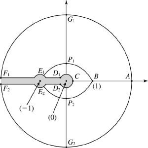
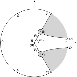
Figure 2: $z$-domain (left) and $\zeta$-domain (right), with corresponding points. These figures were taken from http://dlmf.nist.gov/10.20; they are copyrighted by NIST and used with permission.

Observe that, if we are assuming that the principal values are taken, the expression (3.1) should not be used in all the complex plane and, for instance, for real $z>1$ we would have complex values of $\zeta$, when $\zeta$ should be real for real $z>0$. This problem is solved by taking the following:

$$\frac{2}{3}(-\zeta)^{3/2}=\left(z^{2}-1\right)^{1/2}-\arctan\left\{\left(z^{2}-1\right)^{1/2}\right\},$$ (3.2)

which in fact is an alternative when $\Re z>1$ (and in fact a larger region). We can also write this in terms of logarithms as

$$\zeta(z)=\left\{\begin{array}[]{l}\left(\frac{\displaystyle{3}}{\displaystyle{2}}\right)^{2/3}\left[\log\frac{\displaystyle{1+\sqrt{1-z^{2}}}}{\displaystyle{z}}-\sqrt{1-z^{2}}\right]^{2/3},\,\Re(z)\leq 1,z\notin{\mathbb{R}}^{-},\\ -\left(\frac{\displaystyle{3}}{\displaystyle{2}}\right)^{2/3}\left[i\log\frac{\displaystyle{1+i\sqrt{z^{2}-1}}}{\displaystyle{z}}+\sqrt{z^{2}-1}\right]^{2/3},\,\Re(z)>1.\end{array}\right.$$ (3.3)

We get (1.3), with $u$ replaced by $\nu$, and

$$\psi(\zeta)=\frac{\displaystyle{5}}{\displaystyle{16\zeta^{2}}}+\frac{\displaystyle{\zeta z^{2}(z^{2}+4)}}{\displaystyle{4(z^{2}-1)^{3}}}.$$

From (Olver:1997:ASF, , Chap. 11, §10)) we identify the asymptotic solutions by

$$J_{\nu}(\nu z)=\frac{1}{\nu^{1/3}}\left(\frac{4\zeta}{1-z^{2}}\right)^{1/4}W_{0}(\nu,\zeta),$$ (3.4)

$$H_{\nu}^{(1)}(\nu z)=\frac{2e^{-\pi i/3}}{\nu^{1/3}}\left(\frac{4\zeta}{1-z^{2}}\right)^{1/4}W_{-1}(\nu,\zeta),$$ (3.5)

and

$$H_{\nu}^{(2)}(\nu z)=\frac{2e^{\pi i/3}}{\nu^{1/3}}\left(\frac{4\zeta}{1-z^{2}}\right)^{1/4}W_{1}(\nu,\zeta).$$ (3.6)

For the corresponding Liouville-Green expansions, set

$$\xi=\frac{2}{3}\zeta^{3/2},$$

and define

$$V=\left(\frac{1-z^{2}}{z^{2}}\right)^{1/4}w.$$

For our purposes we only need to consider $\left|\arg(z)\right|\leq\frac{1}{2}\pi$, and so $\arg(\zeta)\leq 0$. Thus, taking $\arg(\xi)=0$ when $\arg(\zeta)=0$, and letting $\xi$ depend continuously on $\zeta$ in the region corresponding to $\left|\arg(z)\right|\leq\frac{1}{2}\pi$, we find that $\arg(\xi)\leq 0$.

We observe then that $\xi\rightarrow+\infty$ as $z\rightarrow 0^{+}$ ($\zeta\rightarrow+\infty)$. Also, $\left|\xi\right|\rightarrow\infty$ as $z\rightarrow i\infty$, such that $\xi=iz-\frac{1}{2}i\pi+\mathcal{O}\left(z^{-1}\right)$ ($\arg(\xi)\rightarrow-\pi)$. In addition, $\left|\xi\right|\rightarrow\infty$ as $z\rightarrow-i\infty$, such that $\xi=iz+\frac{1}{2}i\pi+\mathcal{O}\left(z^{-1}\right)$ ($\arg(\xi)\rightarrow-2\pi)$.

Then we have the transformed equation (1.3), again with $u$ replaced by $\nu$, and

$$\phi(\xi)=\frac{z^{2}(z^{2}+4)}{4(z^{2}-1)^{3}},$$

Now consider the coefficients given by (2.5) - (2.7). In general, we prefer to numerically evaluate with respect to $z$, since $\xi$ is given explicitly in terms of $z$, but not vice versa. Thus, on account of

$$\frac{dz}{d\xi}=-\frac{z}{(1-z^{2})^{1/2}},$$

we have $E_{s}(\xi)=\hat{E}_{s}(z)$ (say), where

$$\hat{E}_{s}(z)=\int_{z}^{\infty}t^{-1}(1-t^{2})^{1/2}\hat{F}_{s}(t)dt\quad(s=1,2,3,\cdots),$$ (3.7)

in which

$$\hat{F}_{s}(z)=F_{s}\left(\xi(z)\right)\quad(s=1,2,3,\cdots).$$

Thus

$$\hat{F}_{1}(z)=\frac{z^{2}(z^{2}+4)}{8(z^{2}-1)^{3}},\,\hat{F}_{2}(z)=\frac{z}{2(1-z^{2})^{1/2}}\hat{F}_{1}^{\prime}(z),$$ (3.8)

and

$$\hat{F}_{s+1}(z)=\frac{z}{2(1-z^{2})^{1/2}}\hat{F}_{s}^{\prime}(z)-\frac{1}{2}\sum_{j=1}^{s-1}\hat{F}_{j}(z)\hat{F}_{s-j}(z)\quad(s=2,3,\cdots).$$ (3.9)

For convenience we have chosen the integration constants so that all coefficients vanish at $z=\infty$.

In the general case, the coefficients $\hat{E}_{s}(z)$ can be computed numerically by quadrature via (3.7). But for Bessel’s equation it turns out that the coefficients can be explicitly computed, and in particular they have the expression

$$\hat{E}_{s}(z)=\frac{P_{s}(z^{2})}{(1-z^{2})^{3s/2}},$$ (3.10)

where $P_{s}(x)$ are polynomials of degree $s$ in $x$.

Before establishing this, we note for the odd terms that

$$\hat{E}_{2j+1}(z)=\frac{1}{(1-z)^{1/2}}\left[\frac{P_{2j+1}(z^{2})}{(1-z^{2})^{3j+1}(1+z)^{1/2}}\right]\ (j=0,1,2\cdots),$$

where the term in the square brackets is meromorphic at $z=1$. Hence, on expanding around the turning point $\zeta=0$ ($z=1$), we deduce that (2.23) holds with $\alpha_{2j+1}=0$, as desired.

In order to establish (3.10), we first show that the coefficients $\hat{F}_{s}(z)$ have the form

$$\hat{F}_{s}(z)=\frac{z^{2}Q_{s}(z^{2})}{(1-z^{2})^{\frac{3}{2}(s+1)}},$$ (3.11)

with $Q_{s}(t)$ a polynomial of degree not larger than $s$ in $t$.

We firstly observe that $\hat{F}_{1}(z)$ has this form. Next, we substitute (3.11) in (3.9) and then, for (3.11) and (3.9) to hold, we have that the polynomials must satisfy

$$Q_{s+1}(t)=\left[1+\frac{1}{2}(3s+1)t\right]Q_{s}(t)+t(1-t)Q_{s}^{\prime}(t)-\frac{t}{2}\sum_{j=1}^{s-1}Q_{j}(t)Q_{s-j}(t),$$ (3.12)

which, starting from $Q_{1}(t)=(1/2+t/8)$, shows that $Q_{n}$ is of degree not larger than $n$ and that (3.11) holds with polynomials given by (3.12).

Now, the coefficients $\hat{E}_{s}$ can be computed from

$$\hat{E}_{s}(z)=-\int_{a}^{z}\hat{F}_{s}(r)\frac{\left(1-r^{2}\right)^{1/2}}{r}dr=-\int_{a}^{z}\frac{rQ_{s}(r^{2})}{(1-r^{2})^{1+3s/2}}dr,$$

where the starting point $a$ is chosen depending on the solution to be matched. These integrals can be explicitly computed. We have

$$\int\frac{rQ_{s}(r^{2})}{(1-r^{2})^{1+3s/2}}dr=\frac{1}{2}\int\frac{{Q_{s}(t)}}{{(1-t)^{1+3s/2}}}dt,$$

and because $Q_{s}$ is a polynomial of degree not larger than $s$ we are left with integrals of the form

$$\int\frac{t^{k}}{(1-t)^{a}}dt=H(t)+C,\,H(t)=\frac{R_{k}(t)}{(1-t)^{a-1}},$$ (3.13)

with $k<a-1$ and $R_{k}$ a polynomial of degree not larger than $k$ which can be computed by differentiating (3.13). Because $k<a-1$, we have $H(\infty)=0$.

The polynomials $P_{s}$ in (3.10) have the properties:

$$P_{2s}(0)=0,\,P_{2s+1}(0)=C_{2s+1},$$

where $C_{2s+1}$ are the coefficients in the Stirling asymptotic series

$$\log{\rm\Gamma}(u)=\left(u-\frac{1}{2}\right)\log(u)-u+\frac{1}{2}\log(2\pi)+\sum_{j=0}^{\infty}\frac{C_{2j+1}}{u^{2j+1}},\,u\rightarrow\infty.$$

We found that the property $P_{2s+1}(0)=C_{2s+1}$ holds by comparing (3.4) with a similar expansion for $J_{\nu}(\nu z)$ but matching the solution at $z=0$, using that $J_{\nu}(\nu z)\sim(\nu z/2)^{\nu}/{\rm\Gamma}(\nu+1)$ as $z\rightarrow 0$.

The first few polynomials are

$$\begin{array}[]{l}P_{1}(x)=\frac{1}{24}(2+3x),\\ \\ P_{2}(x)=-\frac{1}{16}x(x+4),\\ \\ P_{3}(x)=\frac{1}{5760}(-16+1512x+3654x^{2}+375x^{3}),\\ \\ P_{4}(x)=\frac{1}{128}x(32+288x+232x^{2}+13x^{3}).\end{array}$$

Next, using

$$H_{\nu}^{(1)}(\nu z)\sim\left(\frac{2}{\pi\nu z}\right)^{1/2}\exp\left\{i\nu z-\frac{1}{2}\nu\pi i-\frac{1}{4}\pi i\right\},$$

as $z\rightarrow\infty$ we match the solutions that are recessive in the upper half $z$-plane, yielding

$$H_{\nu}^{(1)}(\nu z)=-i\left(\frac{2}{\pi\nu}\right)^{1/2}\frac{1}{(1-z^{2})^{1/4}}V_{-1}(\nu,\xi),$$ (3.14)

as $\nu\rightarrow\infty$, uniformly for $z$ lying in a domain which contains the first quadrant (excluding a neighborhood of the turning point $z=1$).

Furthermore, we know

$$J_{\nu}(\nu z)=\frac{c_{0}(\nu)}{(1-z^{2})^{1/4}}V_{0}(\nu,\xi),$$

as $\nu\rightarrow\infty$ in a domain which contains $\mathrm{Re}(z)\geq 0$, excluding a neighborhood of the interval $[1,\infty)$. Using $\xi=iz-\frac{1}{2}i\pi+\mathcal{O}\left(z^{-1}\right)$, (2.11) and

$$J_{\nu}(\nu z)\sim-\left(\frac{1}{2\pi\nu z}\right)^{1/2}\exp\left\{-i\nu z+\frac{1}{2}\nu\pi i+\frac{1}{4}\pi i\right\},$$

as $z\rightarrow i\infty$, we find that $c_{0}(\nu)=(2\pi\nu)^{-1/2}$, and hence

$$J_{\nu}(\nu z)=\left(\frac{1}{2\pi\nu}\right)^{1/2}\frac{1}{\left(1-z^{2}\right)^{1/4}}V_{0}(\nu,\xi).$$ (3.15)

We remark that the expansions (3.14) and (3.15) are a reformulation of the Debye expansions (Olver:2010:BF, , §10.19(ii)) for $z\in\left(0,1\right)$, which also holds for certain complex values. Debye expansions valid for $1<z<\infty$ are also given in this reference.

4 Bessel’s equation: turning point coefficient functions

We now define the (scaled) turning point coefficient functions for Bessel’s equation. Taking $w_{-1}(u,z)=H_{\nu}^{(1)}(z)$ and $w_{1}(u,z)=H_{\nu}^{(2)}(z)$ in (2.34) these are defined by

$$e^{\pi i/3}H_{\nu}^{(1)}(\nu z)=\mathrm{Ai}_{-1}\left(\nu^{2/3}\zeta\right)\mathcal{A}(\nu,z)+\mathrm{Ai}_{-1}^{\prime}\left(\nu^{2/3}\zeta\right)\mathcal{B}(\nu,z),$$ (4.1)

and

$$e^{-\pi i/3}H_{\nu}^{(2)}(\nu z)=\mathrm{Ai}_{1}\left(\nu^{2/3}\zeta\right)\mathcal{A}(\nu,z)+\mathrm{Ai}_{1}^{\prime}\left(\nu^{2/3}\zeta\right)\mathcal{B}(\nu,z).$$ (4.2)

Comparing these two representations with (3.4) and (3.5) we perceive that in (2.30) the scaling function here is given by

$$\phi(\nu,z)=\frac{2^{3/2}}{\nu^{1/3}}\left(\frac{\zeta}{1-z^{2}}\right)^{1/4}.$$ (4.3)

From (2.14) and (3.15) we also have

$$2J_{\nu}(\nu z)=\mathrm{Ai}\left(\nu^{2/3}\zeta\right)\mathcal{A}(\nu,z)+\mathrm{Ai}^{\prime}\left(\nu^{2/3}\zeta\right)\mathcal{B}(\nu,z).$$ (4.4)

A similar relation for $-2Y_{\nu}(\nu z)$ is obtained by replacing $\mathrm{Ai}$ and its derivative by $\mathrm{Bi}$ and its derivative in (4.4).

As described earlier, the idea for computing the slowly varying coefficients $\mathcal{A}(\nu,z)$ and $\mathcal{B}{(\nu,z)}$ in a region containing the turning point $z=1$ is to invoke Cauchy’s integral formula (2.31). In this, the integration is taken along a positively oriented closed loop containing $z$ in its interior, but not the origin; additionally, it should not cross the negative real axis in the $z$-plane; in this way, we can guarantee that in the $\zeta$ plane we stay away from the shaded region in Fig. 2 (right) and therefore that all the functions appearing in the integration are analytic in a domain containing the path of integration and its interior (and therefore Cauchy’s integral formula holds for this integration path). For our purposes it will be sufficient to consider a circular path of integration in (2.32), which can be centered or not at $z=1$, but which in any case must contain $z=1$, but not $z=0$.

From (2.21), (2.30) and (4.3), we have the following expansion which we use to compute $\mathcal{B}(\nu,z)$ on the path of integration

$$\mathcal{B}(\nu,z)\sim\frac{\displaystyle{2\sqrt{2}\exp\left\{\alpha(\nu,z)\right\}}}{\displaystyle{\nu^{2/3}\zeta^{1/4}(1-z^{2})^{1/4}}}\sinh\left\{\frac{\displaystyle{1}}{\displaystyle{\nu}}\beta(\nu,z)\right\},$$

where, formally,

$$\alpha(\nu,z)=\sum_{j=1}^{\infty}\frac{\hat{E}_{2j}(z)+d_{2j}(\xi)}{\nu^{2j}},$$

and

$$\beta(\nu,z)=\sum_{j=0}^{\infty}\frac{\hat{E}_{2j+1}(z)-d_{2j+1}(\xi)}{\nu^{2j}},$$

in which

$$d_{s}(\xi)=a_{s}/(s\xi^{s}).$$

where $a_{1}=a_{2}=\frac{5}{72},$ and subsequent terms given by (A.2).

We observe that the cancellation of the coefficient as $\nu\rightarrow\infty$ is located in the $\sinh$ term. In order to avoid loss of accuracy, it is better to write

$$\mathcal{B}(\nu,z)\sim\frac{\displaystyle{2\sqrt{2}\beta(\nu,z)\exp\left\{\alpha(\nu,z)\right\}}}{\displaystyle{\nu^{5/3}\zeta^{1/4}(1-z^{2})^{1/4}}}\mathrm{sinhc}\left\{\frac{\displaystyle{\beta(\nu,z)}}{\displaystyle{\nu}}\right\},$$ (4.5)

where the function $\mathrm{sinhc}(x)=\mathrm{sinh}(x)/x$ can be computed for small $x$ with the Maclaurin series

$$\mathrm{sinhc}(x)=\sum_{k=0}^{\infty}\frac{x^{2k}}{(2k+1)!}.$$

Several properties that could be expected for the coefficient $\mathcal{B}(\nu,z)$ can be seen to hold explicitly from (4.5):

1. It is real for real values of $z$.

2. $\mathcal{B}(\nu,z)=\mathcal{O}(\nu^{-5/3})$ as $\nu\rightarrow\infty$, more specifically

   $$\begin{array}[]{ll}\mathcal{B}(\nu,z)&=\frac{\displaystyle{2\sqrt{2}}}{\displaystyle{\nu^{5/3}\zeta^{1/4}(1-z^{2})^{1/4}}}(\hat{E}_{1}(z)-d_{1}(\xi))F(\nu,z)\\ &=\frac{\displaystyle{2\sqrt{2}}}{\displaystyle{\nu^{5/3}\zeta^{1/4}(1-z^{2})^{1/4}}}\left(\frac{\displaystyle{2+3z^{2}}}{\displaystyle{24(1-z^{2})^{3/2}}}-\frac{\displaystyle{5}}{\displaystyle{72\xi}}\right)F(\nu,z),\end{array}$$

   where $F(\nu,z)=1+\mathcal{O}(\nu^{-2})$.

3. Only even powers of $\nu^{-1}$ appear if $F(\nu,z)$ is expanded in powers of $\nu^{-1}$.

Proceeding similarly with the $\mathcal{A}(\nu,z)$ coefficient, we get

$$\mathcal{A}(\nu,z)\sim\frac{\displaystyle{2\sqrt{2}\zeta^{1/4}\exp\left\{\tilde{\alpha}(\nu,z)\right\}}}{\displaystyle{\nu^{1/3}(1-z^{2})^{1/4}}}\cosh\left\{\frac{\displaystyle{1}}{\displaystyle{\nu}}\tilde{\beta}(\nu,z)\right\},$$ (4.6)

where

$$\tilde{\alpha}(\nu,z)=\sum_{j=1}^{\infty}\frac{\hat{E}_{2j}(z)+\tilde{d}_{2j}(\xi)}{\nu^{2j}},$$

$$\tilde{\beta}(\nu,z)=\sum_{j=0}^{\infty}\frac{\hat{E}_{2j+1}(z)-\tilde{d}_{2j+1}(\xi)}{\nu^{2j}},$$

and

$$\tilde{d}_{s}(\xi)=\tilde{a}_{s}/(s\xi^{s}),$$

in which $\tilde{a}_{1}=\tilde{a}_{2}=-\frac{7}{72}$, and subsequent terms satisfying the same recursion formula (A.2) as for the $a_{s}$ coefficients.

For the function $\mathcal{A}(\nu,z)$, we have the expected properties from (4.6):

1. It is real for real values of $z$.

2. $\mathcal{A}(\nu,z)=\mathcal{O}(\nu^{-1/3})$ as $\nu\rightarrow\infty$, more specifically

   $$\mathcal{A}(\nu,z)=\frac{2\sqrt{2}\zeta^{1/4}G(\nu,z)}{\nu^{1/3}(1-z^{2})^{1/4}},$$ (4.7)

   where $G(\nu,z)=1+\mathcal{O}(\nu^{-2})$.

3. Only even powers of $\nu^{-1}$ appear if $G(\nu,z)$ is expanded in powers of $\nu^{-1}$.

For the derivatives ${H_{\nu}^{(1)}}^{\prime}(\nu z)$ and ${H_{\nu}^{(2)}}^{\prime}(\nu z)$ we proceed as before and we express them in the form

$$e^{i\pi/3}\nu{H_{\nu}^{(1)}}^{\prime}(\nu z)=\mathrm{Ai}_{-1}(\nu^{2/3}\zeta)\mathcal{C}(\nu,z)+\mathrm{Ai}_{-1}^{\prime}(\nu^{2/3}\zeta)\mathcal{D}(\nu,z),$$ (4.8)

and

$$e^{-i\pi/3}\nu{H_{\nu}^{(2)}}^{\prime}(\nu z)=\mathrm{Ai}_{1}(\nu^{2/3}\zeta)\mathcal{C}(\nu,z)+\mathrm{Ai}_{1}^{\prime}(\nu^{2/3}\zeta)\mathcal{D}(\nu,z).$$ (4.9)

Solving (4.8) and (4.9) for $\mathcal{C}(\nu,z)$ and $\mathcal{D}(\nu,z)$, and considering the Airy-type expansions for the derivatives (Olver:2010:BF, , 10.20.9), we find that

$$\mathcal{C}(\nu,z)=\mathcal{O}(\nu^{-1/3}),\,\mathcal{D}(\nu,z)=\mathcal{O}(\nu^{1/3}),$$

as $\nu\rightarrow\infty$. From the behavior noted above of $\mathcal{A}(\nu,z)$ and $\mathcal{B}(\nu,z)$ for large $\nu$ (which also hold for their derivatives), we see that in the dominant coefficient $\mathcal{D}(\nu,z)$ the first term in (2.37) is the largest, which is indeed $\mathcal{O}(\nu^{1/3})$, while for the coefficient $\mathcal{C}(\nu,z)$ both terms in (2.36) are $\mathcal{O}(\nu^{-1/3})$, which is the correct order of this coefficient. Therefore, once the cancellation for the coefficient $\mathcal{B}(\nu,z)$ is avoided, no cancellations occur as $\nu\rightarrow\infty$, and we expect both (2.36) and (2.37) to be numerically stable.

There are two possible approaches in numerically evaluating the coefficients $\mathcal{C}(\nu,z)$ and $\mathcal{D}(\nu,z)$. With $\mathcal{A}(\nu,z)$ and $\mathcal{B}(\nu,z)$ computed on the path of integration as described above, the first method is to numerically evaluate the integrals (2.39) and (2.40).

Alternatively, one can use (2.36) and (2.37), with ${\mathcal{A}}(\nu,z)$ and $\mathcal{B}(\nu,z)$, and their derivatives, computed via Cauchy integral formulas. Then, $\zeta$ and $\zeta^{\prime}$ can be evaluated directly from (3.1), (3.2) and (3.3). There is, however, a possible loss of accuracy as $z\rightarrow 1$ in the computation of $\zeta^{\prime}(z)$ but it can be easily eliminated. We have

$$\zeta^{\prime}(z)=-\frac{\left(1-z^{2}\right)^{1/2}}{z\zeta^{1/2}},$$

and both the numerator and the denominator tend to $0$ as $z\rightarrow 1$ which implies loss of accuracy. In order to avoid this we put $\delta=\sqrt{1-z^{2}}$ and when $|\delta|$ is small we consider the Maclaurin series for

$$f(\delta)=\frac{3^{1/3}}{\delta}\left(\log\left(\frac{1+\delta}{\sqrt{1-\delta^{2}}}\right)-\delta\right)^{1/3}=1+\frac{1}{5}d^{2}+\frac{18}{175}d^{4}+\ldots$$

and compute

$$\zeta^{\prime}(z)=-\frac{2^{1/3}}{zf(\delta)}.$$ (4.10)

Returning to $\mathcal{A}(\nu,z)$ and $\mathcal{B}(\nu,z)$, we end this section describing a more direct, but less stable, method for their computation (again, on the path of integration of (2.31)). From (4.1) and (4.2) we have the exact representations

$$\begin{array}[]{ll}\mathcal{A}(\nu,z)=-2\pi i&\left\{e^{i\pi/3}H_{\nu}^{(1)}(\nu z)\mathrm{Ai}_{1}^{\prime}(\nu^{2/3}\zeta)\right.\\ &\left.-e^{-i\pi/3}H_{\nu}^{(2)}(\nu z)\mathrm{Ai}_{-1}^{\prime}(\nu^{2/3}\zeta)\right\},\end{array}$$ (4.11)

and

$$\begin{array}[]{ll}\mathcal{B}(\nu,z)=2\pi i&\left\{e^{i\pi/3}H_{\nu}^{(1)}(\nu z)\mathrm{Ai}_{1}(\nu^{2/3}\zeta)\right.\\ &\left.-e^{-i\pi/3}H_{\nu}^{(2)}(\nu z)\mathrm{Ai}_{-1}(\nu^{2/3}\zeta)\right\}.\end{array}$$ (4.12)

Now, because we are assuming that a method to compute the Airy functions is available (we are precisely considering expansions in terms of Airy functions), we could compute these coefficients on the Cauchy contour without the need to substitute the Airy functions by their Liouville-Green expansions, as done before. For examples of Fortran implementations of complex Airy functions see Amos:1986:A6A ; Fabijonas:2004:A8A ; Gil:2002:A8A .

As before, the integration path is chosen in such a way that the functions appearing in (4.11) and (4.12) can be computed without recourse to the Airy-type expansion. With respect to the cylinder functions involved in the computation of the coefficients, we use (3.14) and (3.15), along with $H_{\nu}^{(2)}(\nu z)=\overline{H_{\nu}^{(1)}(\nu\overline{z})}$.

In order to compute the coefficients in a numerically stable way along the contour of integration, we need to verify that the two terms are not suffering cancellations, which would happen if the two terms are exponentially large and cancel each order. If both Hankel functions are large, one should be replaced by the $J$ Bessel function. For example, we see that inside the eye-shaped curve (Fig 2), the expression for $\mathcal{B}(\nu,z)$ in (4.12) is unstable because two exponentially large quantities are subtracting: all terms in this expression are dominant inside the eye-shaped curve. Outside the eye, this expression is in principle stable because in each term a dominant function multiples a recessive function.

Inside the eye we can write a satisfactory expression using $H_{\nu}^{(2)}(\nu z)=2J_{\nu}(\nu z)-H_{\nu}^{(1)}(\nu z)$. We obtain

$$\mathcal{B}(\nu,z)=2\pi i\left\{H_{\nu}^{(1)}(\nu z)\mathrm{Ai}_{0}(\nu^{2/3}\zeta)-2e^{-i\pi/3}J_{\nu}(\nu z)\mathrm{Ai}_{-1}(\nu^{2/3}\zeta)\right\}.$$ (4.13)

This expression not only can be used inside the eye-shaped region, but also for the rest of the half plane $\Im(z)\geq 0$; however, close to the real axis when $z>1$ we get higher accuracy from Liouville-Green expansions using (4.12). In our numerical algorithms we use (4.12) when $\Re\left(z\right)>1$ and (4.13) in the rest of this half plane. But, as described before, if we also expand the Airy functions instead of computing them separately, we obtain asymptotic expansions for the coefficient away from the turning point and switching from one expression to the other for the coefficients is not needed in this case. See Sect. 4.

Similarly for $\mathcal{A}(\nu,z)$ we have

$$\mathcal{A}(\nu,z)=-2\pi i\left\{H_{\nu}^{(1)}(\nu z)\mathrm{Ai}_{0}^{\prime}(\nu^{2/3}\zeta)-2e^{-i\pi/3}J_{\nu}(\nu z)\mathrm{Ai}_{-1}^{\prime}(\nu^{2/3}\zeta)\right\}.$$

We could do analogous substitutions to get a satisfactory formula when $\Im z\leq 0$. However this is not really necessary because the coefficients $\mathcal{A}(\nu,z)$ and $\mathcal{B}(\nu,z)$ are real on the real line and, as commented before, analytic in a domain containing the integration path. Therefore, by Schwarz reflection principle, in this domain $\mathcal{A}(\nu,\bar{z})=\overline{\mathcal{A}(\nu,z)}$ and $\mathcal{B}(\nu,\bar{z})=\overline{\mathcal{B}(\nu,z)}$. From a computational point of view, this reduces by one half the complexity of evaluating the Cauchy integral, provided we take a symmetric contour with respect to the real axis, as we will do.

This more direct approach has some disadvantages with respect to the expansions in terms of stability. First, we notice that, even when the solutions are chosen adequately, there still remains some cancellation in the $\mathcal{B}(\nu,z)$ coefficient for large orders. Additionally, there is also some accuracy degradation in the computation of Airy functions for large arguments due to unavoidable loss of accuracy in the computation of exponentials of large argument, as we next describe.

5 Numerical results

We now give several numerical illustrations for the performance of both the Liouville-Green expansions and the approximation around the turning point. For this purpose, we have coded our algorithms in Fortran 90, and compared with the values given by Amos’ algorithm (which has typically 13-14 digits accuracy). Amos’ algorithm uses a variety of methods for computing Bessel functions, depending on the values of $\nu$ and $z$, and in particular Airy-type expansions close to the turning point. We have also tested our methods using Maple^TM. The comparison with Amos’ algorithm is used as an exhaustive testbench of the numerical stability of our approximations in fixed precision arithmetic; both Amos’ program and our the implementation are fast enough to provide many thousands of function values in just a second. The tests in variable precision with Maple^TM are much slower and much less exhaustive, but they will allow us to explore higher accuracies.

5.1 Testing of the new Liouville-Green approximations

Here we numerical evaluate the new expansions (3.14) and (3.15). We notice that the analytic continuation formulas of (Olver:2010:BF, , §10.11) can be used to compute cylinder functions for $\Re z<0$ from the values for $\Re z>0$. For instance, we have

$$J_{\nu}(ze^{\pm\pi i})=e^{\pm\nu\pi i}J_{\nu}(z).$$

Therefore, testing for $\Re z>0$ is enough. However, we are also considering the case $\Re z<0$ for the case of $J_{\nu}(z)$ in order to show the full validity region of the expansion (3.15).

A test of the performance of the truncated expansion

$$J_{\nu}(\nu z)\approx\left(\frac{1}{2\pi\nu}\right)^{1/2}\frac{1}{\left(1-z^{2}\right)^{1/4}}\exp\left\{-\nu\xi+\displaystyle\sum_{s=1}^{n}(-1)^{s}\frac{E_{s}(\xi)}{\nu^{s}}\right\},$$ (5.1)

can be seen in Fig. 3. The figure shows the comparison of the function values obtained with $n=14$ in (5.1) against those obtained with Amos’ algorithm Amos:1986:A6A for computing $J_{\nu}(\nu z)$ with $\nu=100$. Fig. 3 shows the comparison for random values of the variable $z$ generated in the domain $-2<\Re{z}<2,\,-2<\Im z<2$, respectively. The points where the relative error is greater than $10^{-12}$ are plotted in the figures. As the figure shows, and as expected, the Liouville-Green expansion (3.15) loses accuracy close to the turning point and for real values of $z$ with $|z|>1$. It is worth noting than in the neighborhood of the turning point we can consider our expansions with coefficients computed via Cauchy integrals that we are discussing next, while for $z>1$ we can compute $J_{\nu}(\nu z)$ using its relation with Hankel functions and the Liouville-Green expansions for these functions or, alternatively, we can use (4.4) with coefficients computed from its asymptotic approximation. It appears then that for $\nu\geq 10$ it is possible to compute $J_{\nu}(\nu z)$ in the whole complex $z$-plane with around $15$ digits accuracy only by resorting to asymptotic approximations.

Finally, the performance of the Liouville-Green approximation

$$H_{\nu}^{(1)}(\nu z)\approx-i\left(\frac{2}{\pi\nu}\right)^{1/2}\frac{1}{\left({1-z^{2}}\right)^{1/4}}\exp\left\{\nu\xi+\displaystyle\sum_{s=1}^{n}\frac{E_{s}(\xi)}{\nu^{s}}\right\},$$ (5.2)

for $\Im z>0$, with again $n=14$, is illustrated in Fig. 4. As expected, the expansion fails in the proximity of $z=1$.

Figure 3: Comparison of the function values obtained with the expansion (3.15) against those obtained with Amos’ algorithm Amos:1986:A6A for computing $J_{\nu}(\nu z)$ with $\nu=100$ and $-2<\Re{z}<2,\,-2<\Im z<2$. The points where the relative error is greater than $10^{-12}$ are plotted.

Figure 4: Comparison of the function values obtained with the expansion (3.14) against those obtained with Amos’ algorithm Amos:1986:A6A for computing $H^{(1)}_{\nu}(\nu z)$ with $\nu=100$ and $0<\Re{z}<2,\,0<\Im z<2$. The points where the relative error is greater than $10^{-12}$ are plotted.

5.2 Airy-type expansions via Cauchy’s integral formula

We now test the accuracy in the computation of the Airy type expansion (4.1) for $H_{\nu}^{(1)}(\nu z)$. We employ two different approaches in the approximation of the coefficient functions $\mathcal{A}(\nu,z)$ and $\mathcal{B}(\nu,z)$, both of which use the Cauchy integral formulas (2.31). In the first approach, on the Cauchy contour we use the Liouville-Green expansions only for the cylinder functions, and we assume an algorithm for computing complex Airy functions is available; we have used both Amos’ algorithm Amos:1986:A6A and our own algorithm Gil:2002:A8A , with similar results. Thus, in (4.1) $\mathcal{A}(\nu,z)$ and $\mathcal{B}(\nu,z)$ (expressed by the appropriate Airy and cylinder functions) are approximated by using the Liouville-Green expansions (5.1) and (5.2) in the integrands of (2.31), but with the Airy functions computed from the algorithms cited.

The second approach uses the Liouville-Green approximations for both the Airy functions and the cylinder functions in approximating $\mathcal{A}(\nu,z)$ and $\mathcal{B}(\nu,z)$ in (4.1) (although again we do use Airy algorithms to compute $\mathrm{Ai}_{-1}\left(\nu^{2/3}\zeta\right)$ and $\mathrm{Ai}_{-1}^{\prime}\left(\nu^{2/3}\zeta\right)$ when computing $H_{\nu}^{(1)}(\nu z)$ with (5.3)). Hence in this case, from (4.1), (4.5) and (4.6), we have for $z$ inside $\mathcal{L}$

$$e^{i\pi/3}H_{\nu}^{(1)}(\nu z)\approx\mathrm{Ai}_{-1}\left(\nu^{2/3}\zeta\right)\mathcal{A}_{m}(\nu,z)+\mathrm{Ai}_{-1}^{\prime}\left(\nu^{2/3}\zeta\right)\mathcal{B}_{m}(\nu,z),$$ (5.3)

where

$$\mathcal{A}_{m}(\nu,z)=\frac{1}{2\pi i}\oint\limits_{\mathcal{L}}\frac{\displaystyle{2\sqrt{2}\zeta^{1/4}\exp\left\{\tilde{\alpha}_{m}(\nu,t)\right\}}}{\displaystyle{\nu^{1/3}(1-t^{2})^{1/4}(t-z)}}\cosh\left\{\frac{\displaystyle{1}}{\displaystyle{\nu}}\tilde{\beta}_{m}(\nu,t)\right\}dt,$$ (5.4)

$$\mathcal{B}_{m}(\nu,z)=\frac{1}{2\pi i}\oint\limits_{\mathcal{L}}\frac{\displaystyle{2\sqrt{2}\beta_{m}(\nu,t)\exp\left\{\alpha_{m}(\nu,t)\right\}}}{\displaystyle{\nu^{5/3}\zeta(t)^{1/4}(1-t^{2})^{1/4}(t-z)}}\mathrm{sinhc}\left\{\frac{\displaystyle{\beta_{m}(\nu,t)}}{\displaystyle{\nu}}\right\}dt,$$ (5.5)

in which

$$\tilde{\alpha}_{m}(\nu,t)=\sum_{j=1}^{m}\frac{\hat{E}_{2j}(t)+\tilde{d}_{2j}\left(\xi(t)\right)}{\nu^{2j}},$$

$$\tilde{\beta}_{m}(\nu,t)=\sum_{j=0}^{m-1}\frac{\hat{E}_{2j+1}(t)-\tilde{d}_{2j+1}\left(\xi(t)\right)}{\nu^{2j}},$$

$$\alpha_{m}(\nu,t)=\sum_{j=1}^{m}\frac{\hat{E}_{2j}(t)+d_{2j}\left(\xi(t)\right)}{\nu^{2j}},$$

and

$$\beta_{m}(\nu,t)=\sum_{j=0}^{m-1}\frac{\hat{E}_{2j+1}(t)-d_{2j+1}\left(\xi(t)\right)}{\nu^{2j}}.$$

Two different tests of the accuracy of the Airy-type asymptotic expansion for $H_{\nu}^{(1)}(\nu z)$ (with coefficients evaluated by Cauchy’s integral formula), for $z$ fixed or $\nu$ fixed, are considered. The results are shown in Fig. 5, for which the Airy function has been evaluated both using Gil:2002:A8A and Amos:1986:A6A , with similar results. In all cases we take $m=7$, which means we are considering terms up to $\mathcal{O}(\nu^{-n})$, $n=2m=14$. Of course, similar tests can be made for other solutions of the Bessel equation (for instance $J_{\nu}(\nu z)$ or $Y_{\nu}(\nu z)$), and the accuracy results are very similar, as can be expected since all solutions are computed with the same coefficients.

In Fig. 5, the relative error in the comparison of the function values obtained with the Airy-type expansion for $H_{\nu}^{(1)}(\nu(1+0.1i)),\,2<\nu<400$ against those obtained with Amos’ algorithm is shown. Several different sources of error are apparent in the figure: the error for $\nu$ small due to the Liouville-Green approximations for cylinder functions used in the Airy-type expansions, the small increase in the error due to rounding for $\nu$ large caused by the $\mathcal{B}(\nu,z)$ coefficient, and the unavoidable loss of accuracy in the computation of Airy functions for large arguments.

Figure 5: Relative errors in the comparison of the function values obtained with the Airy-type expansion with $n$ terms for $H^{(1)}_{\nu}(\nu(1+0.1i))$ against those obtained with Amos’ algorithm Amos:1986:A6A . In the evaluation of the coefficients the Airy functions are also computed with Amos:1986:A6A

In Fig. 6 we show the same results as in Fig. 5, but using the asymptotic expansions for the coefficients given in Sect. 4. We observe a clear improvement over Fig. 5, particularly for low $\nu$. As $\nu$ becomes larger, there a slow increase in accuracy loss (smaller than in the previous case). This is due to the increasing inaccuracies in the computation of Airy functions as the argument becomes larger, which give rise to errors in the computation of the Hankel function when using (4.1). These inaccuracies are unavoidable in finite precision arithmetic and, as described in Gil:2002:A8A , can only be removed by considering scaled functions (with the dominant exponential factor exactly scaled out).

Figure 6: Relative errors in the comparison of the function values obtained with the Airy-type expansion for $H^{(1)}_{\nu}(\nu(1+0.1i))$ against those obtained with Amos’ algorithm Amos:1986:A6A . The asymptotic expansion of the coefficients is considered over the Cauchy contour. We take $n=14=2m$ in Eqs. (5.4) and (5.5).

Figure 7: Same as Fig. 6 but for smaller $\nu$ and four selections of $n=2m$: $n=6,10,14,18$.

Figure 8: Comparison of the function values obtained with the Airy-type expansion for $H^{(1)}_{10}(10z)$ against those obtained with Amos’ algorithm Amos:1986:A6A . The points where the relative error is greater than $10^{-13}$ are plotted. We take $n=2m=14$.

Fig. 7 shows the same tests, but focusing in smaller values of $\nu$ and for two selections in the number of terms for the expansion. We observe two tendencies, particularly for $n=2m=18$: a decrease of the error as $\nu$ increases due to the fact that the expansion becomes more accurate, and a slow increase of the error due to the finite precision computation of the Airy functions in the expression for $H^{(1)}_{\nu}(\nu z)$; this error increase is not attributable to our approach. These tendencies give an optimal accuracy for $\nu$ close to $5$. As commented, the accuracy for larger $\nu$ in finite precision arithmetic can be improved by considering scaled functions.

In Fig. 8 we plot the points where the relative error is greater than $10^{-13}$ in the comparison of the function values obtained with the Airy-type expansion for $H^{(1)}_{10}(10z)$ against those obtained with Amos’ algorithm. The random $z$ points in the test have been generated inside the semi-circle limited by the integration contour used to compute the coefficient functions $A(\nu,z)$ and $B(\nu,z)$ of the Airy-type asymptotic expansion (a circle of center $z_{c}=2$ and radius $R=1.8$). As can be seen in the figure, the accuracy obtained with the expansion is better than $10^{-13}$ in a large portion of the domain although, as expected, it worsens when approaching the integration contour. This figure illustrates the accuracy in the discretization of the Cauchy integral in a large region, but with $z$ not too close to the contour of integration.

Preliminary tests show that the time spent for the computation of the Liouville-Green expansions in §3 and the Airy-type expansions in §4 is similar to the time for the implementations of Debye and Airy-type expansions in Amos’ algorithm Amos:1986:A6A . However, as expected, when the Cauchy’s integral formula is used our approach becomes slower for computing a single function value, because we need to compute the coefficients a number of times over the contour.

The advantage of the Cauchy approach is that the most costly computation is the evaluation of the coefficients $E_{j}(\xi)$ and the numerators in the sums of Eqs. (2.20) and (2.21), but this computation is done once and for all over the contour. Our approach permits the selection of a convenient Cauchy contour depending on the application. If many functions values are needed in a certain $z$-region, a good approach is to precompute the coefficients in a circuit containing this region (if it is possible and the shaded regions of Fig. 2 can be avoided), and then applying the discretized version of Cauchy integral formula (Eq. (2.33)) as many times as needed (and the recomputation of the sums in Eqs. (2.20) and (2.21) if $\nu$ is also varying).

At this point, it is important to stress that the main interest of the Cauchy technique lies in the computability more than in the efficiency (although it is efficient). It provides a new and direct method of computation of the coefficients of Airy-type expansions with potential applications to more complicated cases.

In addition to the tests in fixed precision arithmetic, we have performed additional test in variable precision using Maple^TM. Firstly, we have checked that the coefficients in the Airy-type expansions are computed in a numerically stable way with our scheme and that the remaining error degradation in Fig. 6 is due to loss of accuracy in the computation of the Airy functions when using (5.3). For this purpose, we have used Maple^TM for computing the coefficients with a fixed number of digits (we take 16 digits) and then computed the Hankel function using (5.3) with a sufficiently high number of digits. When we test the value of the Hankel function with, say $50$ digits, we observe that the error is always close to $16$ digits accuracy, which shows that the coefficients have been consistently computed with that accuracy and without accuracy loss for high $\nu$. This is illustrated in Fig. 9.

Figure 9: Error in the computation of $H_{\nu}^{(1)}(\nu z)$ for $z=1+0.1i$ when the coefficients over the Cauchy contour are computed with $16$ digits and using their LG asymptotic expansion. The rest of computations are performed with $50$ digits using Maple. As before, $n=14$.

In all the computations, we have used $500$ points in the contour of integration. The error associated with the discretization of the Cauchy integral is so small that it has no impact on the previous results. For observing this error, a higher number of digits should be considered. Fig. 10 shows the results when $500$ points over the Cauchy contour are considered and the computations are done with $50$ digits.

Figure 10: Error in the computation of $H_{\nu}^{(1)}(\nu z)$ for $z=1+0.1i$ and various selections of $n=2m$ when the coefficients over the Cauchy contour and the rest of computation are performed with $50$ digits using Maple. The limit in the minimal possible error (close to $10^{-26}$) is due to the discretization of the Cauchy integral with $N=500$ points

As can be expected, because the integrand is periodic, the trapezoidal rule has exponential convergence. Indeed, we have checked that smallest reachable error roughly depends on the number of points over the Cauchy contour as $10^{-N/20}$.

We have checked numerically that when the effect of discretization of the Cauchy integral is negligible, the relative error when $n$ terms in the asymptotic expansion of the coefficients are considered, the relative error in the computation of $H^{(1)}_{\nu}(\nu z)$ close to the turning point varies as $C_{n+1}/\nu^{n+1}$, where $C_{n+1}$ does not depend on $\nu$ and increases with $n$. This is the expected behavior for an asymptotic expansion for large $\nu$. Some estimations of these constants close to $z=1$ are shown in table 1

$$\begin{array}[]{lllllllll}\hline\cr n&4&6&8&10&12&14&16&18\\ \hline\cr C_{n+1}&0.00015&0.00013&0.00021&0.00051&0.0018&0.0089&0.056&0.46\\ \hline\cr\end{array}$$

Table 1: Computational error constants for the computation of $H^{(1)}_{\nu}(\nu z)$ close to $z=1$. The relative error is in good approximation given by $C_{n+1}/\nu^{n+1}$

It would be important to be able to establish strict error bounds and to compare them with these experimental errors. This should be achievable by bounding the errors in the Liouville-Green expansions used for the coefficients, similar to the error bounds given in Dunster:1998:AOT , and again appealing to Cauchy’s integral formula. This will be considered in a subsequent paper.

Appendix A Appendix: Exponential-form expansions for Airy functions

Firstly, the Airy functions $\mathrm{Ai}_{j}\left(u^{2/3}\zeta\right)$ satisfy

$$d^{2}w/d\zeta^{2}=u^{2}\zeta w.$$ (A.1)

Letting $\xi=\int\zeta^{1/2}d\zeta=\frac{2}{3}\zeta^{3/2}$ (as in (2.1)), we then have that the functions $V=\zeta^{1/4}\mathrm{Ai}_{j}\left(u^{2/3}\zeta\right)$ satisfy

$$\frac{d^{2}V}{d\xi^{2}}=\left\{u^{2}-\frac{5}{36\xi^{2}}\right\}V.$$

An asymptotic solution of the form (2.4) now applies. In particular, on identifying solutions of (A.1) that are recessive at $\zeta=+\infty$, we have that there exists a constant $c(u)$ such that

$$\mathrm{Ai}\left(u^{2/3}\zeta\right)\sim c(u)\zeta^{-1/4}\exp\left\{-u\xi+\displaystyle\sum_{s=1}^{\infty}(-1)^{s}\frac{e_{s}(\xi)}{u^{s}}\right\},$$

as $u^{2/3}\zeta\rightarrow\infty$ in the sector $\left|\arg\left(\zeta\right)\right|\leq\pi-\delta$ ($\delta>0)$.

The coefficients in this expansion are given by (2.5) - (2.7), with $E$ and $F$ replaced by $e$ and $f$, respectively, and $\phi(\xi)=-\frac{5}{{36}}\xi^{-2}$. In particular, $e_{s}(\xi)=\int_{\infty}^{\xi}f_{s}(t)dt$, where

$$f_{1}(\xi)=-\frac{5}{72\xi^{2}},\quad f_{2}(\xi)=-\frac{5}{72\xi^{3}},$$

and

$$f_{s+1}(\xi)=-\frac{1}{2}f_{s}^{\prime}(\xi)-\frac{1}{2}\displaystyle\sum_{j=1}^{s-1}f_{j}(\xi)f_{s-j}(\xi)\quad(s\geq 2).$$

Thus

$$f_{s}(\xi)=-\frac{a_{s}}{\xi^{s+1}},\quad e_{s}(\xi)=\frac{a_{s}}{s\xi^{s}}\quad(s=1,2,3,\cdots),$$

where $a_{1}=a_{2}=\frac{5}{72}$, and

$$a_{s+1}=\frac{1}{2}(s+1)a_{s}+\frac{1}{2}\displaystyle\sum_{j=1}^{s-1}a_{j}a_{s-j}\quad(s\geq 2).$$ (A.2)

From the well-known leading term

$$\mathrm{Ai}\left(u^{2/3}\zeta\right)\sim\frac{e^{-u\xi}}{2\pi^{1/2}u^{1/6}\zeta^{1/4}}\quad\left(u^{2/3}\zeta\rightarrow\infty\right),$$

we obtain $c(u)=1/\left(2\pi^{1/2}u^{1/6}\right)$, and hence we deduce that

$$\mathrm{Ai}\left(u^{2/3}\zeta\right)\sim\frac{1}{2\pi^{1/2}u^{1/6}\zeta^{1/4}}\exp\left\{-u\xi+\displaystyle\sum_{s=1}^{\infty}(-1)^{s}\frac{a_{s}}{su^{s}\xi^{s}}\right\},$$ (A.3)

which is uniformly valid for $\left|\arg\left(\zeta\right)\right|\leq\pi-\delta$ ($\delta>0$). Expansions for $\mathrm{Ai}_{\pm 1}\left(u^{2/3}\zeta\right)$ can be obtained directly from this.

Next, from differentiating (A.1) we find that $y=\zeta^{-1/2}\mathrm{Ai}_{j}^{\prime}\left(u^{2/3}\zeta\right)$ satisfy

$$\frac{d^{2}y}{d\zeta^{2}}=\left\{u^{2}\zeta+\frac{3}{4\zeta^{2}}\right\}y.$$

Thus, again with $\xi=\frac{2}{3}\zeta^{3/2}$, we have that $\tilde{V}=\zeta^{-1/4}\mathrm{Ai}_{j}^{\prime}\left(u^{2/3}\zeta\right)$ satisfy

$$\frac{d^{2}\tilde{V}}{d\xi^{2}}=\left\{u^{2}+\frac{7}{36\xi^{2}}\right\}\tilde{V}.$$

Similarly to (A.3), on using (Olver:2010:AAR, , (9.7.6)), we deduce that

$$\mathrm{Ai}^{\prime}\left(u^{2/3}\zeta\right)\sim-\frac{u^{1/6}\zeta^{1/4}}{2\pi^{1/2}}\exp\left\{-u\xi+\displaystyle\sum_{s=1}^{\infty}(-1)^{s}\frac{\tilde{a}_{s}}{su^{s}\xi^{s}}\right\},$$ (A.4)

for $\left|\arg(\zeta)\right|\leq\pi-\delta$, where $\tilde{a}_{1}=\tilde{a}_{2}=-\frac{7}{72}$, and subsequent terms also satisfy (A.2). Expansions for $\mathrm{Ai}_{\pm 1}^{\prime}\left(u^{2/3}\zeta\right)$ can be obtained directly from this.

- (1) Amos, D.E.: Algorithm 644: a portable package for Bessel functions of a complex argument and nonnegative order. ACM Trans. Math. Software 12(3), 265–273 (1986)
- (2) Amos, D.E., Daniel, S.L., Weston, M.K.: CDC 6600 subroutines IBESS and JBESS for Bessel functions and . ACM Trans. Math. Software 3(1), 76–92 (1977)
- (3) Bornemann, F.: Accuracy and stability of computing high-order derivatives of analytic functions by Cauchy integrals. Found. Comput. Math. 11(1), 1–63 (2011)
- (4) Boyd, W.G.C.: Asymptotic expansions for the coefficient functions that arise in turning-point problems. Proc. Roy. Soc. London Ser. A 410(1838), 35–60 (1987)
- (5) Dunster, T.M.: Asymptotics of the eigenvalues of the rotating harmonic oscillator. J. Comput. Appl. Math. 93(1), 45–73 (1998)
- (6) Fabijonas, B.R.: Algorithm 838: Airy functions. ACM Trans. Math. Software 30(4), 491–501 (2004)
- (7) Gil, A., Segura, J., Temme, N.M.: Algorithm 819: AIZ, BIZ: two Fortran 77 routines for the computation of complex Airy functions. ACM Trans. Math. Software 28(3), 325–336 (2002)
- (8) Gil, A., Segura, J., Temme, N.M.: Numerical methods for special functions. SIAM, Philadelphia, PA (2007)
- (9) Olver, F.W.J.: Asymptotics and special functions. AKP Classics. A K Peters Ltd., Wellesley, MA (1997). Reprint of the 1974 original [Academic Press, New York]
- (10) Olver, F.W.J.: Airy and related functions. In: NIST handbook of mathematical functions, pp. 193–213. U.S. Dept. Commerce, Washington, DC (2010)
- (11) Olver, F.W.J., Maximon, L.C.: Bessel functions. In: NIST handbook of mathematical functions, pp. 215–286. U.S. Dept. Commerce, Washington, DC (2010)
- (12) Temme, N.M.: Numerical algorithms for uniform Airy-type asymptotic expansions. Numer. Algorithms 15(2), 207–225 (1997)