Approximating Certain Cell-Like Maps by Homeomorphisms^‡

Abstract.

Given a proper map $f:M\rightarrow Q$, having cell-like point-inverses, from a manifold-without-boundary $M$ onto an ANR $Q$, it is a much-studied problem to find when $f$ is approximable by homeomorphisms, i.e., when the decomposition of $M$ induced by $f$ is shrinkable (in the sense of Bing). If dimension $M\geq 5$, J. W. Cannon’s recent work focuses attention on whether $Q$ has the disjoint disc property (which is: Any two maps of a 2-disc into $Q$ can be homotoped by an arbitrarily small amount to have disjoint images; this is clearly a necessary condition for $Q$ to be a manifold, in this dimension range). This paper establishes that such an $f$ is approximable by homeomorphisms whenever dimension $M\geq 5$ and $Q$ has the disjoint disc property. As a corollary, one obtains that given an arbitrary map $f:M\rightarrow Q$ as above, the stabilized map $f\times id(\mathbb{R}^{2}):M\times\mathbb{R}^{2}\rightarrow Q\times\mathbb{R}^{2}$ is approximable by homeomorphisms. The proof of the theorem is different from the proofs of the special cases in the earlier work of myself and Cannon, and it is quite self-contained. This work provides an alternative proof of L. Siebenmann’s Approximation Theorem, which is the case where $Q$ is given to be a manifold.







The Edwards’ Manuscript Project. This article is one of three highly influential articles on the topology of manifolds written by Robert D. Edwards in the 1970’s but never published. This article “Approximating certain cell-like maps by homeomorphisms”presents the definitive theorem on the recognition of high-dimensional manifolds among resolvable generalized manifolds. The theorem says that every cell-like map from an $n$-manifold ($n\geq 5$) to an ANR is approximable by homeomorphisms provided that the ANR has the disjoint disc property. (This work garnered Edwards an invitation to give a one-hour plenary address to the 1978 International Congress of Mathematicians.) The second article “Suspensions of homology spheres”presents the initial solutions of the fabled Double Suspension Conjecture. The third article “Topological regular neighborhoods”develops a comprehensive theory of regular neighborhoods of locally flatly embedded topological manifolds in high dimensional topological manifolds. The manuscripts of these three articles have circulated privately since their creation. The organizers of the Workshops in Geometric Topology (http://sites.coloradocollege.edu/geometrictopology2016/) with the support of the National Science Foundation have facilitated the preparation of electronic versions of these articles to make them publicly available. Preparation of the electronic manuscripts was supported by NSF Grant DMS-0407583. Final editing was carried out by Fredric Ancel, Craig Guilbault and Gerard Venema.

1. Introduction

Approximation Theorem: Suppose $f:M\rightarrow Q$ is a proper cell-like map from a manifold-without-boundary $M$ onto an ANR $Q$, and suppose that $Q$ has the disjoint disc property and that $\dim M\geq 5$. Then $f$ is arbitrarily closely approximable by homeomorphisms. Stated another way, the decomposition of $M$ induced by $f$ is shrinkable (in the sense of Bing).

2. Shrinking Certain 0-dimensional decompositions

The goal of this section is to prove the following theorem. We are assuming for proofs that M is compact.

$\boldsymbol{0}$-Dimensional Shrinking Theorem. Suppose $f:M\rightarrow Q$ is a cell-like map of a manifold $M$ onto a quotient space $Q$, and suppose

• the image of the nondegeneracy set of $f$ has dimension 0, and

• the nondegeneracy set of $f$ has codemension $\geq 3$ in $M$.

Then the decomposition of $M$ induced by $f$ is shrinkable; that is, $f$ is arbitrarily closely approximable by homeomorphisms.

Note. There is no dimension restriction on $M$ in this theorem (or anywhere in this section). Nor is there any restriction on the $closure$ in $Q$ of the image of the nondegeneracy set - it may be all of $Q$. This is why the theorem will be useful, in sections 3 and 4.

The above theorem will be derived from the following theorem, which amounts to the special case when the decomposition is countable and null.

Countable Shrinking Theorem. Suppose $f:M\rightarrow Q$ is a cell-like map of a manifold $M$ onto a quotient space $Q$, and suppose

• the nontrivial point-inverses of $f$ comprise a countable null collection, where null means that their diameters tend to 0, and

• each nontrivial point-inverse of $f$ has codimension $\geq 3$ in M.

Then the decomposition of $M$ induced by $f$ is shrinkable; that is, $f$ is arbitrarily closely approximable by homeomorphisms.

Notes.

(1). Both of these theorems are false when codimension $\geq 3$ is replaced by codimension $\geq 2$, even assuming $f$ is cellular. In dimension 3, Bing’s countable planar-Knaster-continua decomposition [Bi2] provides a counterexample to the two theorems. In dimensions $\geq 4$, Eaton’s generalized dogbone space [Ea] provides a counterexample to the first theorem, and a modification of this example, implicit in the first proof below, provides a counterexample to the second theorem.

(2). As an incidental fact, recall that in either theorem, even without conditions (2), the quotient space $Q$ is necessarily an ANR, since by hypothesis $Q$ is a union of two finite dimensional subsets (namely, the image of the nondegeneracy set of $f$, and its complement), hence $Q$ is finite dimensional. (See [Hu-Wa].)

Proof that Countable Shrinking Theorem $\Rightarrow$ 0-Dimensional Shrinking Theorem. In brief, the idea is to tube together the nontrivial point inverses of $f$ in such a manner as to come up with a countable null collection. (This sort of operation, for the closed-0-dimensional situation, was done in [Ea-Pi] and Lemma 2 of [Ed-Mi], and probably elsewhere, too.)

The rationale is this. Given $f:M\rightarrow Q$ as in the first theorem, suppose that for any $\epsilon>0$ one can come up with a quotient map $g:Q\rightarrow Q_{\#}$, with point-inverses of diameter $<\epsilon$, such that the composition $gf:M\rightarrow Q_{\#}$ is approximable by homeomorphisms. (In our case, this will be because $gf$ satisfies the Countable Shrinking Theorem). Then $f$ is approximable by homeomorphisms. This is an easy, and fairly well-known, consequence of the Bing Shrinking Criterion. (On the other hand, I do not see any easy proof which does not use the BSC.)

We proceed with the proof. If the nondegeneracy set of the given map $f:M\rightarrow Q$ were compact, we would argue as follows. Given $\epsilon>0$, let $\{U_{i}|1\leq i\leq p\}$ be a finite cover of the 0-dimension image of nondeg$(f)$ by disjoint open subsets of $Q$ of diameter $<\epsilon$. Fixing $i$, let $\{N_{j}|1\leq j<\infty\}$ be a strictly decreasing sequence of compact, not-necessarily-connected manifold neighborhoods of nondeg$(f)\cap f^{-1}(U_{i})$ in $f^{-1}(U_{i})$, such that $\cap^{\infty}_{j=1}N_{j}=\mbox{nondeg}(f)\cap f^{-1}(U_{i})$, and such that each component of each $N_{j}$ is null-homotopic in $N_{j-1}$. (Read $f^{-1}(U_{i})$ for $N_{0}$ here.) (The $N_{j^{\prime}s}$ can be chosen to be manifolds because without loss $f^{-1}(U_{i})$ is a PL manifold, since each point inverse of $f$, being cellular by say [Mc], has a PL manifold neighborhood.)

To connect the $N_{j}$’s, we start with $j=1$, and proceed in increasing order of the $j$’s, joining the components of $N_{j}$ together by tubes in $int\;N^{\#}_{j-1}$ (let $N^{\#}_{0}$ be $P^{-1}(U_{i})$ here), to get a compact connected manifold $N^{\#}_{j}$ which is null-homotopic in $N^{\#}_{j-1}$. Then let $Y_{i}=\cap^{\infty}_{j=1}N^{\#}_{j}$, which is a cell-like set containing nondeg$(f)\cap f^{-1}(U_{i})$. We can assume $Y_{i}$ has codemension $\geq 3$, because the connecting operation can be done carefully so that, for example, $Y_{i}-\mbox{nondeg}(f)$ has countably many components, each a locally flatly embedded interval. Let $Q_{\#}$ be the quotient space $M/\{Y_{i}|1\leq i\leq p\}$. Then the quotient map $g:Q\rightarrow Q_{\#}$ serves as the map $g$ in the preceding paragraph.

In the general case, when the nondegeneracy set of the given map $f:M\rightarrow Q$ is not compact, but only $\sigma$-compact, one essentially does a countable number of connecting operations as above, first for the 1-nondegeneracy set of $f$, then for the 1/2-nondegeneracy set of $f$, etc., where the $\epsilon$-nongeneracy set of $f$ is the compact set $\cup\{f^{-1}(q)|\mbox{diam}f^{-1}(q)\geq\epsilon,q\epsilon Q\}$. But some care, and explanation, is required. First, a little care is necessary to ensure that the new intervals, which are introduced to connect nontrivial point-inverses of $f$, miss all of the original nontrivial point-inverses. This is easily done, using the codemension hypothesis. The second point, requiring explanation, is more fundamental. One can do the connecting operation on the 1-nondegeneracy set, then on the 1/2-nondegeneracy set minus the new 1-nondegeneracy set, then on the 1/3-nondegeneracy set minus the new 1/2-nondegeneracy set, etc., and this will produce a countable upper semi-continuous decomposition, but it may not be null, since at the second stage one may actually be producing a countable number of new nondegenerate point-inverses of diameter $\geq 1/2$. One way to get around this is, when working on the 1/2-nondegeneracy set, to allow the finitely many already-constructed new 1-nondegenerate point-inverses to enlarge a little, by connecting to them the 1/2-nondegenerate point-inverses which are sufficiently close. This way one can arrange to have only finitely many 1/2-nondegenerate point-inverses at the end of the second stage. At the next stage, one again allows an arbitrarily small enlargement of the already constructed 1/2-nondegenerate point-inverses, so as to wind up with only a finite number of 1/3-nondegenerate point-inverses. Since the amount of enlarging is arbitrarily small at each stage, one can arrange in the limit that the nondegenerate point-inverses be cell-like and codemension $\geq 3$, as well as countable and null.

The following rigorization of the above proof turns out to be a little bit different in detail, but is the same in spirit, and has the virtue of relative brevity. Basically, the idea is to intertwine the choice of the connecting tubes with the choice of the manifold neighborhood sequence.

Let $N_{1}$ be a not-necessarily-connected compact manifold neighborhood of 1-nondeg$(f)$, so small that each component of $N_{1}$ $(i)$ lies in the 1-neighborhood of some point-inverse in 1-nondeg$(f)$, and $(ii)$ has image in $Q$ of diameter $<\epsilon$ (where $\epsilon>0$ is given at the start, as explained earlier). Let $N_{2}=N_{2,a}\cup N_{2,b}$ be a not-necessarily-connected compact manifold neighborhood of 1/2-nondeg$(f)$, where $N_{2,a}$ and $N_{2,b}$ are disjoint and each is a union of components of $N_{2}$, so small that each component of $N_{2}$ $(i)$ lies in the 1/2-neighborhood of some point-inverse in 1/2-nondeg$(f)$, and $(ii)$ has image in $Q$ of diameter $<\epsilon$, and so that $(iii)$ $N_{2,a}$ is a neighborhood of 1-nondeg$(f)$, $(iv)$ each component of $N_{2,a}$ lies in, and is null homotopic in, some component of $N_{1}$ (but the components of $N_{2,b}$ may have no relation to $N_{1}$ at all), and $(v)$ each component of $N_{2,b}$ has diameter $<1$. One way to do all of this choosing is first to find a partitioning $f$(1/2-nondeg$(f))=C_{2,a}\cup C_{2}$ of the image of the 1/2-nondegeneracy set of $f$ into two disjoint closed (0-dimensional) subsets $C_{2,a}$ and $C_{2,b}$ such that 1-nondeg$(f)\subset f^{-1}(C_{2,a})\subset\;int\;N_{1}$. Then choose in the quotient $Q$ two disjoint open neighborhoods $U_{2,a}$ of $C_{2,a}$ and $U_{2,b}$ of $C_{2,b}$, so small that the preimages $f^{-1}(U_{2,a})$ and $f^{-1}(U_{2,b})$ and their components satisfy conditions $(i)-(v)$ above. Now let $N_{2,a}$ be any compact manifold neighborhood of 1/2-nondeg$(f)\cap f^{-1}(U_{2,a})$ in $f^{-1}(U_{2,a})$, and likewise choose $N_{2,b}$.

At this time, we tube together the various components of $N_{2,a}$ which lie in a common component of $N_{1}$ (but the components of $N_{2,b}$) are not tubed together). We would like these tubes to miss $N_{2,b}$; a priori that may not be possible, because $N_{2,b}$ may disconnect some of the components of $N_{1}$. So what we do is first to choose the various connecting tubes in $N_{1}-\;int\;N_{2,a}$, so thin and well-positioned that they miss 1/2-nondeg$(f)$, but possibly may intersect $N_{2,b}$, and then we throw away from $N_{2,b}$ a small neighborhood of the intersection of the tubes with $N_{2,b}$, producing a smaller manifold $N^{\prime}_{2,b}$ which can take the place of $N_{2,b}$. Finally, let $N^{*}_{2}$ denote the union of $N^{\prime}_{2,b}$ and the tubed-together components of $N_{2,a}$. So $N^{*}_{2}$ has one component for each component of $N_{1}$, and one component for each component of $N^{\prime}_{2,b}$.

This process is now repeated, to construct $N^{*}_{3},N^{*}_{4}$, etc. To save words, let it suffice to say that, in order to construct $N^{*}_{i+1}$ given $N^{*}_{i}$, the above procedure works word-for-word, after making the substitution $N^{*}_{i}$ for $N_{1}$; $N_{i+1}$, $N_{i+1,a}$ and $N_{i+1,b}$ for $N_{2},N_{2,a}$ and $N_{2,b}$ and likewise for the $C$’s and $U$’s; $N^{*}_{i+1}$ for $N^{*}_{2}$; and elsewhere $1/i$ for $1$ and $1/(i+1)$ for $1/2$. (The very first substitution listed is the single exception to the general theme $1\rightarrow i$ and $2\rightarrow i+1$.)

As part of the construction, one is obtaining at each stage an injective correspondence $\alpha_{i}:$ components of $N^{*}_{i}\rightarrow$ components of $N^{*}_{i+1}$, such that for any component $P$ of $N^{*}_{i}$, $\alpha_{i}(P)$ is null-homotopic in $P$. Hence for each $P,\cap^{\infty}_{j=i}\alpha_{j}(\alpha_{j-1}(\ldots(\alpha_{i}(P))\ldots))$ is a cell-like set, $P^{*}$ say, of codemension $\geq 3$ by the usual additional case. (This latter claim uses $(i)$, to conclude that the set $P^{*}$ minus the 1-demensional connecting intervals in $P^{*}$ lies in nondeg$(f)$, hence the codemension $\geq 3$). Then the null collection $\{P^{*}\}$ consisting of all of these cell-like sets, exactly one for each component of each difference manifold $N^{*}_{i}-\cup\alpha_{i-1}$ (components of $N^{*}_{i-1}$), $i\geq 2$ (let $N^{*}_{1}=\emptyset$ here), is the desired null collection. This completes the proof that Countable Shrinking Theorem $\Rightarrow$ 0-Dimensional Shrinking Theorem.

Proof of the Countable Shrinking Theorem. Let $\{Y_{1},Y_{2},\ldots\}$ be the countable null collection of disjoint codimension $\geq 3$ cell-like sets in $M$, which are the nontrivial point-inverses of $f$. Our goal is to prove:

Shrinking Lemma: Given any $Y_{i}$ and any $\epsilon>0$, there is a neighborhood $U$ of $Y_{i}$, $U\subset N_{\epsilon}(Y_{i})$, and there is a homeomorphism $h:M\rightarrow M$, supported in $U$, such that for any $Y_{j}$, if $h(Y_{j})\cap U\neq\emptyset$, then $diam$ $h(Y_{j})<\epsilon$.

Technical Note. The reason for writing $h(Y_{j})\cap U\neq\emptyset$ instead of the equivalent $Y_{j}\cap U\neq\emptyset$, is to make this statement more nearly resemble that of the a-Shrinking Lemma, below.

Given this Lemma, it is an easy matter to show that the Bing Shrinking Criterion holds for the given decomposition $f:M\rightarrow M/\{Y_{i}\}=Q$ as in [Bi1]. For given $\epsilon>0$, the BSC is that there exist a homeomorphism $h:M\rightarrow M$ such that $(i)$ $dist(fh,f)<\epsilon$, and $(ii)$ for each $Y_{i}$, $diam$ $h(Y_{i})<\epsilon$. Such an $h$ can be gotten by applying the above Shrinking Lemma to sufficiently small disjoint neighborhoods of the finitely many $Y_{i}$’s which initially have diameter $\geq\epsilon$.

As an introduction to the proof of the Shrinking Lemma, we consider the trivial demension range case, where each $Y_{i}$ satisfies $2\,dem\,Y_{i}+2\leq m$. In this case, to prove the Lemma for $Y_{i}$ say, one starts by embedding $cY_{i}$ (the cone on $Y_{i}$) in $N_{\epsilon}(Y_{i})$, extending the given embedding $Y_{i}\hookrightarrow N_{\epsilon}(Y_{i})$ of its base $Y_{i}$, so that $dem\,cY_{i}\leq dem\,Y_{i}+1$. (If $2\,dem\,Y_{i}+3\leq m$, this is a classical result of Menger-Nöbeling [Hu-Wa]; if $2\,dem\,Y_{i}+2=m$, see the next paragraph for how to do something just as good.) Then, by general position applied a countable number of times, one can ambient isotope $cY_{i}$ an arbitrarily small amount, keeping its base $Y_{i}$ fixed, to make $cY_{i}$ disjoint from all of the other $Y_{j}$’s. Thus, one now has a guideway in $M$ minus the other $Y_{j}$’s, namely $cY_{i}$, along which to shrink $Y_{i}$. Of course, the other $Y_{j}$’s may converge closer and closer to $cY_{i}$, but as they do so, they must get smaller and smaller, by their nullity. The exact method of constructing the shrinking homeomorphism $h$ at this point is modeled on Bing’s original work, and is discussed fully in the following paragraphs.

Given a cellular set $Y$ in $M$ (for example, a codemension $\geq 3$ cell-like set) and a neighborhood $U$ of $Y$, we can find a coordinate chart $\mathbb{R}^{m}\hookrightarrow M$ of $M$ lying in $U$ such that $Y\subset int\;B^{m}$, where $B^{m}$ is the unit ball in the coordinate chart, and also origin $0\notin Y$. (We hope the reader will be able to tolerate this frequently-occurring abuse of notation, namely out not labeling the embedding $R^{m}\hookrightarrow M$. This will leave upcoming expressions much less cluttered.) Let $Y_{1}\subset\partial B^{m}$ denote the image of $Y$, projected from the origin. (Similarly, for upcoming use, let $Y_{r}\subset\partial\,rB^{m}$ denote the projected image of $Y$, where $rB^{m}$ is the ball of radius $r>0$.)

Lemma. By an arbitrarily small perturbation of the coordinate chart embedding, we can arrange that dem $Y_{1}\leq$ dem $Y$.

To minimize ambiguity here, we emphasize that $Y$, being regarded as a subset of $M$, is left fixed; it is only the coordinate chart embedding $\mathbb{R}^{m}\hookrightarrow M$ that is being changed, in order to change what (the preimage of) $Y$ looks like in $\mathbb{R}^{m}$. Note that some perturbing may be necessary; even a tame cantor set $Y$ in int $B^{m}-0$ can have its projection-image $Y_{1}$ be all of $\partial B^{m}$.

Proof of Lemma: If $Y$ were a locally flatly (on each open stratum) embedded polyhedron in int $B^{m}$, one could achieve the Lemma by making $Y$ PL embedded in $B^{m}$ (PL on each open stratum would suffice). The general proof is the demension theory analogue of this. Actually, it is quickest to think in terms of complements. Let $K=L^{m-y-2}\cup\infty$ be a countable union of $(m-y-2)$-sphere on $\partial B^{m}\approx\mathbb{R}^{m-1}\cup\infty$, where $y=\dim Y$, gotten from the countable union of $(m-y-2)$-planes in $\mathbb{R}^{m-1}$ consisting of all points of $\mathbb{R}^{m-1}$ having at least $y+1$ coordinates rational. (Thus $\partial B^{m}-K\approx\mathbb{R}^{m-1}-L$ is Nöbeling’s $y$-dimensional space.) Any compact subset of $\partial B^{m}-K$ has demension $\leq y$. To arrange that $Y_{1}\subset\partial B^{m}-K$, one applies general position, perturbing the coordinate chart embedding on int$B^{m}$ to make $cK$ (which has dimension $m-y-1$) disjoint from $Y$. $\blacksquare$

Assuming then that dem $Y_{1}\leq$ dem $Y$, let $X=cY_{1}$, that is, $Y_{1}$ coned to the origin in $B^{m}$. By construction, dem $X\leq$ dem $Y+1$. (For upcoming use let $rX=cY_{r}$; it has the same demension as $X$).

To such an $X$, we associate a fixed sequence of special compact neighborhoods $N_{1}\supset int\;N_{1}\supset N_{2}\supset\ldots$ of $X$ in $M$, with $X=\cap_{\ell=1}^{\infty}N_{\ell}$, constructed as follows. Let $O_{1}\supset int\;O_{1}\supset O_{2}\supset\ldots$ be any strictly decreasing sequence of compact neighborhoods of $Y_{1}$ in $\partial B^{m}$ such that $Y_{1}=\cap_{\ell=1}^{\infty}O_{\ell}$. Define $N_{\ell}=c(1+1/\ell)O_{\ell}\cup 1/\ell B^{m}$, that is, $N_{\ell}$ is the cone (to the origin) on the projection image $(1+1/\ell)O_{\ell}\subset\partial(1+1/\ell)B^{m}$, together with the $m$-ball of radius $1\ell$. (See Figure 1).

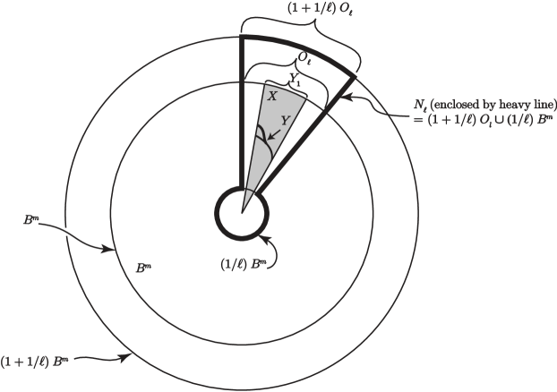
Figure 1.

We emphasize that given $Y$, once its associated $X$ and its neighborhood sequence $\{N_{\ell}\}$ have been constructed, they are fixed entities for the duration of the proof (except that perhaps certain arbitrarily small general positioning ambient isotopies may be applied to them).

We now describe the fundamental squeezing homeomorphism that will be used throughout the proof. Given $X$ and $\{N_{\ell}\}$ as above, and given a finite indexing subsequence $\lambda:\{1,\ldots,p\}\rightarrow\{p,p+1,\ldots\}$ of length $p$, where $p\geq 2$ is arbitrary, say $\lambda:p\leq\lambda(1)<\lambda(2)<\ldots<\lambda(p)$, we define a specific homeomorphism $h_{\lambda}:M\rightarrow M$ which will have the following properties:
$(i)$ $h_{\lambda}$ is fixed off of $N_{\lambda(1)}$ and on $1/\lambda(1)B^{m}$,
$(ii)$ $h_{\lambda}$ is radial and inward-moving in the coordinate chart structure, i.e., each radial line segment in $2B^{m}$ is carried onto itself by $h_{\lambda}$, and each point, if moved, is moved toward the origin,
$(iii)$ $h_{\lambda}(X)\subset 2/p\,B^{m}$, and
$(iv)$ for any connected subset $C$ of $M$ which intersects at most a single $fr\,N_{\lambda(j)}$, the radial-height of $C$ (defined below) is increased by at most $4/p$ under $h_{\lambda}$. Hence, if such a subset $C$ lying in the coordinate patch $\mathbb{R}^{m}\hookrightarrow M$ has euclidean-metric diameter $\leq\eta$, then $h_{\lambda}(C)$ has euclidean-metric diameter $\leq\eta+4/p$.

The radial height of $C$ is the length of the projection of $C\cap\mathbb{R}^{m}$ onto the radius coordinate $[0,\infty)$ in the coordinate chart $\mathbb{R}^{m}\hookrightarrow M$. (Since $C$ is connected, this projection-image of $C\cap\mathbb{R}^{m}$ is an interval. To be technically complete, let us agree that in the special case when this image is the interval $[c,\infty)$, then $(iv)$ above means that the projection-image of $h(C)\cap\mathbb{R}^{m}$ lies in $[c-4/p,\infty)$.)

On each radial line segment of $2B^{m}$, $h_{\lambda}$ will be piecewise linear, with at most $p+1$ “breaks” (changes in derivative); they will be at the (source) levels $\partial(1+1/\lambda(j))B^{m}$, $1\leq j\leq p$, and at $\partial(1/\lambda(1))B^{m}$. Let these $p+1$ decreasing radii be $s(1),\ldots,s(p+1)$. That is, for each $j,1\leq j\leq p$, let $s(j)=1+1/\lambda(j)$, and let $s(p+1)=1/\lambda(1)$. Let $t(1),\ldots,t(p+1)$ be the $p+1$ equally spaced numbers decreasing from $1+1/\ell(1)$ to $1/\ell(1)$; inclusive. That is, if each $j,1\leq j\leq p+1$, let $t(j)=1+1/\lambda(1)-(j-1)/p$. The general idea is to have $h_{\lambda}$ carry the $s$-levels to the $t$-levels. We start by defining $h_{\lambda}$ on the “outer end” of each $N_{\lambda(j)}$, namely on $s(j)O_{\lambda(j)}$, so that $h_{\lambda}(s(j)O_{\lambda(j)}=t(j)O_{\lambda(j)}$. (Necessarily then the image $h_{\lambda}(N_{\lambda(j)})$ must be $ct(j)O_{\lambda(j)}\cup 1/\lambda(1)B^{m}$.) Next, define $h_{\lambda}$ on the cylindrical sleeve $[s(p+1),s(1)](O_{\lambda(j)}-int\;O_{\lambda(j+1)}),1\leq j\leq p$, (here $[a,b]O$ denotes $cl(bO-aO)$, and $O_{\lambda(p+1)}=\phi)$ one at a time, in order of increasing $j$. At the $j$th stage, $h_{\lambda}$ has already been defined on $[s(p+1),s(1)]fr\;O_{\lambda(j)}$, and has there $j+1$ breaks (or no breaks, if $j=1$), at the $j+1$ (source) levels $s(1)fr\;O_{\lambda(j)},\ldots,s(j)fr\;O_{\lambda(j)},s(p+1)fr\;O_{\lambda(j)}$, which are taken respectively by $h_{\lambda}$ to the $j+1$ (target) levels $t(1)fr\;O_{\lambda(j)}\ldots,t(j)fr\;O_{\lambda(j)},t(p+1)fr\;O_{\lambda(j)}$. Define

$$h_{\lambda}|[s(j), s(1)](O_{\lambda(j)}-int\;O_{\lambda(j+1)})=$$

$$h_{\lambda}|[s(j),s(1)]fr\;O_{\lambda(j)}\times\;\mbox{identity}(O_{\lambda(j)}-int\;O_{\lambda(j+1)}),$$

where the meaning of this expression should be clear. In order to define $h_{\lambda}$ on the remaining region $[s(p+1),s(j)](O_{\lambda(j)}-int\;O_{\lambda(j+1)})$ to complete this stage of the definition, we must choose a Urysohn function to tell us where to send the level $s(j+1)(O_{\lambda(j)}-int\;O_{\lambda(j+1)})$. Let

$$\phi:s(j+1)(O_{\lambda(j)}-int\;O_{\lambda(j+1)})\longrightarrow[t(j+1),t(j)]$$

be a map such that $\phi|s(j+1)fr\;O_{\lambda(j)}=$ the radius value of $h_{\lambda}(s(j+1)fr\;O_{\lambda(j)})$ (which one may compute) and $\phi|s(j+1)fr\;O_{\lambda(j+1)}=t(j+1)$. Then define $h_{\lambda}$ on the level $s(j+1)(O_{\lambda(j)}-int\;O_{\lambda(j+1)})$ by $h_{\lambda}(s(j+1)x)=\phi(x)\cdot x$ for each $x\in O_{\lambda(j)}-int\;O_{\lambda(j+1)}$. Finally extend $h_{\lambda}$ in linear fashion over each radial line segment on the regions $[s(p+1),s(j+1)](O_{\lambda(j)}-int\;O_{\lambda(j+1)})$ and $[s(j+1),s(j)](O_{\lambda(j)}-int\;O_{\lambda(j+1)})$. This completes the definition of $h_{\lambda}$.

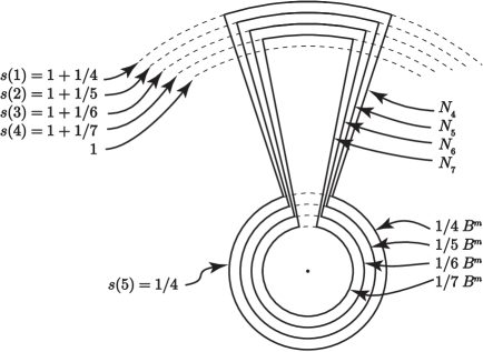
Before applying $h_{\lambda}$

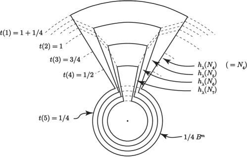
After applying $h_{\lambda}$

Figure 2. The squeezing homeomorphism $h_{\lambda}$. Pictured here is the case $p=4=\lambda(1)<\dots<\lambda(4)=7$.

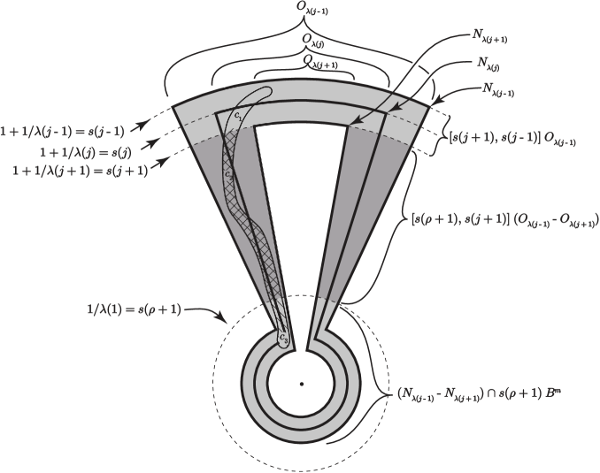
Figure 3.

The only nontrivial property of $h_{\lambda}$ to verify is $(iv)$, and that can be understood by looking at Figures 2 and 3. The $h_{\lambda}$-image of an arbitrary connected set $C\subset N_{\lambda(j-1)}-N_{\lambda(j+1)}$ can be analyzed by breaking $C$ into three pieces. First there is $C_{1}\equiv C\cap[s(j+1),s(j-1)]O_{\lambda(j-1)}$, whose image under $h_{\lambda}$ has radial height $\leq 2/p$. Then there is $C_{2}\equiv C\cap[s(p+1),s(j+1)](O_{\lambda(j-1)}-O_{\lambda(j+1)})$. On each radial interval of $[s(p+1),s(j+1)](O_{\lambda(j-1)}-O_{\lambda(j+1)})$ $h_{\lambda}$ is linear (and compressing), fixed on the inner end of the interval, while all of the outer ends (i.e., $s(j+1)(O_{\lambda(j-1)}-O_{\lambda(j+1)})$ have their images under $h_{\lambda}$ in the region $[t(j+1),t(j-1)]B^{m}$. So the radial height of $C_{2}$ is increased by at most $2/p$, which is the difference between $t(j-1)$ and $t(j+1)$. Finally, there is $C_{3}\equiv C\cap s(p+1)B^{m}$, which is left fixed by $h_{\lambda}$. Combining these facts, one obtains property $(iv)$. This completes our discussion of the standard squeezing homeomorphism $h_{\lambda}$.

We return for a moment to the trivial demension range case, when $2\;dem\;Y_{i}+2\leq m$ for each $i$, to illustrate exactly how the above-constructed shrinking homeomorphism will be called into play. Having fixed $i$ and $\epsilon>0$, earlier we said to nicely embed $cY_{i}$ in $N_{\epsilon}(Y_{i})$; now instead we find a cone $X_{i}=cY_{i,1}$ containing $Y_{i}$, constructed as above so that $dem\>X_{i}\leq dem\>Y_{i}+1$ by working in a coordinate chart of $M$ which lies in $N_{\epsilon}(Y_{i})$. As earlier, $X_{i}$ can be general positioned to intersect none of the other $Y_{j}^{\prime}s$. Let $\{N_{\ell}\}$ be a fixed sequence of neighborhoods of $X_{i}$, constructed as above. The goal now is to choose $p\geq 2$ and a subsequence $\lambda:p\leq\lambda(1)<\lambda(2)<\ldots<\lambda(p)$ so that the associated squeezing homeomorphism $h_{\lambda}$ satisfies the conclusion of the Shrinking Lemma. The precise way to choose this subsequence $\lambda$ is explained in the proof of the following Proposition. We emphasize that in this Proposition, all distances are measured in the given metric on the manifold $M$.

Squeezing Proposition. Suppose $X\subset M$ is any compact cone lying in a coordinate chart of $M$ as described above (that is, $X=c(X\cap\partial B^{m})$, where $B^{m}$ is the standard $m$-ball in the coordinate chart), and suppose $\{N_{\ell}|1\leq\ell<\infty\}$ is a sequence of compact neighborhoods of $X$ as described above. Then given $\epsilon>0$ there exists $\delta>0$ and an integer $p\geq 2$ such that for any subsequence $\lambda:p\leq\lambda(1)<\lambda(2)<\ldots<\lambda(p)$ of integers, the squeezing homeomorphism $h_{\lambda}$ (described above) has the following properties:
(1) $diam\>h_{\lambda}(X)<\epsilon$, and
(2) for any connected subset $C$ of $M$ such that $diam\>C<\delta$ and $C$ intersects at most one of the sets $fr\>N_{\lambda(j)}$, $1\leq j\leq p$, one has that $diam\>h_{\lambda}(C)<\epsilon.$

Proof. The proof of properties (1) and (2) rests on the fact that the two metrics on $\mathbb{R}^{m}\hookrightarrow M$, the one induced from the $M$-metric and the other being the standard euclidean metric, are equivalent. Since $h_{\lambda}$ has support in $2B^{m}$, let us assume without loss that the set $C$ of (2) lies in $3B^{m}$. Given $\epsilon>0$, let $\epsilon^{\prime}>0$ be such that any subset of $3B^{m}$ having euclidean-metric-diameter $<\epsilon^{\prime}$ has $M$-metric-diameter $<\epsilon$. Let $\delta^{\prime}>0$ and $p\geq 2$ be such that $\delta^{\prime}+4/p<\epsilon^{\prime}$. Finally, let $\delta>0$ be such that any subset of $3B^{m}$ having $M$-metric-diameter $<\delta$ has euclidean-metric-diameter $<\delta^{\prime}$. Now given any sequence $\lambda:p\leq\lambda(1)<\ldots<\lambda(p)$, and given any connected set $C$ as in the proposition, $C\subset 3B^{m}$, then the euclidean-metric-diameter of $C$ is $<\delta^{\prime}$, and hence the euclidean-metric-diameter of $h_{\lambda}(C)$ is $\delta^{\prime}+4/p<\epsilon^{\prime}$, and hence the $M$-metric-diameter of $h_{\lambda}(C)$ is $<\epsilon$. $\blacksquare$

In order to prove the general codemension 3 case of this theorem, we do an iterated general positioning operation, just as in the proof of codemension $\geq 3$ engulfing. The inductive hypothesis is provided by the following Lemma; the Shrinking Lemma above can be thought of as the $A=M$ case of this Lemma.

$\boldsymbol{a}$-Shrinking Lemma $(-1\leq a\leq m-2)$. Suppose $A$ is a closed subset of $M$, with dem $A\leq a$. Given any $Y_{i}$ and any $\epsilon>0$, there is a neighborhood $U$ of $Y_{i},U\subset N_{\epsilon}(Y_{i})$, and there is a homeomorphism $h:M\rightarrow M$, supported in $U$, such that for any $Y_{j}$, if $h(Y_{j})\cap U\cap A\neq\varnothing$, then diam $h(Y_{j})<\epsilon$.

This will be proved by induction on increasing $a$. But first we illustrate the general idea by establishing that $(m-2)$-Shrinking Lemma $\Rightarrow$ Shrinking Lemma. We point out, for the reader who would like to gain familiarity with the entire proof a step at a time (as I did), that
(1) In the trivial dimension range case, when $2y+2\leq m$, where $y=\max\{dem\>Y_{i}\}$, one is in effect only using the a-Shrinking Lemma for $a\leq y+1$, whose proof is a trivial general position argument, already used, together with the proof that $(y+1)$-Shrinking Lemma $\Rightarrow$ Shrinking Lemma, as below.
(2) in the “metastable” dimension range case, when $3y+4\leq 2m$ ($y$ as above), one is in effect only using the a-Shrinking Lemma for $a\leq y+1$, whose proof in turn only uses the a-Shrinking Lemma for $a\leq 2y+3-m$, whose proof is the aforementioned trivial general position argument, together with the proof that $(y+1)$-Shrinking Lemma $\Rightarrow$ Shrinking Lemma, as below.

Proof that $\boldsymbol{(m-2)}$-Shrinking Lemma $\Rightarrow$ Shrinking Lemma. Denote by $Y_{0}$ the given $Y_{i}$ in the Shrinking Lemma. Given $\epsilon>0$, let $U_{0}\subset N_{\epsilon}(Y_{0})$ be a saturated neighborhood of $Y_{0}$ (saturated meaning that if any $Y_{j}$ intersects $U_{0}$, it lies in $U_{0}$), so small that if $Y_{j}\subset U_{0}$, $Y_{j}\neq Y_{0}$, then $diam\;Y_{j}<\epsilon$. In $U_{0}$, choose a coordinate patch of $M$ containing $Y_{0}$, and construct there in the manner explained earlier a cone $X_{0}$ containing $Y_{0}$, with dem $X_{0}\leq dem\;Y_{0}+1\leq m-2$, and a special neighborhood basis $\{N_{\ell}\}$ of $X_{0}$. Let $\delta>0$ and $p\geq 2$ be as provided by the Proposition , for this data (without loss $\delta<\epsilon)$. Our goal is to move off of $X_{0}$ those intersecting $Y_{j}$’s (other than $Y_{0}$) which are too big, by using the $(m-2)$-Shrinking Proposition, leaving behind to intersect $X_{0}$ only $Y_{j}$-images of size $<\delta$. Then we iterate this operation $p-1$ more times in order to achieve the desired insulation of $X_{0}$ from $M-N_{\lambda(1)}$. We remark now that, even though these various moves in the successive stages may have overlapping supports, their composition will not stretch any $Y_{j}$ to have diameter $\geq\epsilon$.

To start, let $\mathscr{Y}_{1}$ be the finite subcollection of members of $\mathscr{Y}-\{Y_{0}\}$ which intersect $X_{0}$ and have diameter $\geq\delta$. (Here $\mathscr{Y}$ denotes the entire collection $\{Y_{i}\}$.) Choose a collection $\mathscr{U}_{1}$ of disjoint open saturated neighborhoods of the members of $\mathscr{Y}_{1}$, each member of $\mathscr{U}_{1}$ having diameter $<\epsilon$ and lying in $U_{0}-Y_{0}$. For each member $U$ of $\mathscr{U}_{1}$, apply the $(m-2)$-Shrinking Lemma, with $\epsilon$-value $\min\{\delta,dist\,(\cup\,\mathscr{Y}_{1},M-\cup\,\mathscr{U}_{1})\}$, to find a homeomorphism $h_{U}$, supported in $U$, such that the $h_{U}$-image of any member of $\mathscr{Y}$ lying in $U$ and intersecting $X_{0}$ has diameter $<\delta$. Letting $H_{1}$ be the composition of these $h_{U}$’s, $U\in\mathscr{U}_{1}$, it follows that each member of $H_{1}(\mathscr{Y}-\{Y_{0}\})$ which intersects $X_{0}$ has diameter $<\delta$. So we can choose $\lambda(1)\geq p$ so large that $N_{\lambda(1)}\subset U_{0}$ and each member of $H_{1}(\mathscr{Y}-\{Y_{0}\})$ which intersects $N_{\lambda(1)}$ has diameter $<\delta$,

From now on, the repeating steps are qualitatively the same, but they are a little bit different from the just-completed first step. Let $\mathscr{Y}_{2}$ be the finite subcollection of members of $H_{1}(\mathscr{Y}-\{Y_{0}\})$ which intersect both $fr\,N_{\lambda(1)}$ and $X_{0}$. (Possibly $\mathscr{Y}_{2}\cap H_{1}(\mathscr{Y}_{1})\neq\varnothing$; that is allowable.) Choose a collection $\mathscr{U}_{2}$ of disjoint open $H_{1}(\mathscr{Y})$-saturated neighborhoods of the members of $\mathscr{Y}_{2}$, each having diameter $<\delta$ (which is $<\epsilon$) and lying in $U_{0}-Y_{0}$. For each member $U$ of $\mathscr{U}_{2}$, apply the $(m-2)$-Shrinking Lemma, with $\epsilon$-value $\min\{dist\,(X_{0},M-N_{\lambda(1)}),dist\,(\cup\,\mathscr{Y}_{2},M-\cup\,\mathscr{U}_{2})\}$, to find a homeomorphism $h_{U}$, supported in $U$, such that the $h_{U}$-image of any member of $H_{1}(\mathscr{Y})$ which intersects $X_{0}$ necessarily misses $fr\,N_{\lambda(1)}$. Letting $H_{2}$ be the composition of these $h_{U}$’s, $U\in\mathscr{U}_{2}$, it follows that each member of $H_{2}H_{1}(\mathscr{Y}-\{Y_{0}\})$ which intersects $N_{\lambda(1)}$ has diameter $<\delta$, and also each member of $H_{2}H_{1}(\mathscr{Y})$ intersects at most one of $fr\,N_{\lambda(1)}$ and $X_{0}$. We can now choose $\lambda(2)>\lambda(1)$ so large that each member of $H_{2}H_{1}(\mathscr{Y})$ intersects at most one of $fr\,N_{\lambda(1)}$ and $fr\,N_{\lambda(2)}$.

In general, the argument goes as follows. (The following $k=2$ case was done above). Given $k,\ 2\leq k\leq p$, suppose we have constructed a homeomorphism $G_{h-1}(=H_{k-1}\circ\ldots\circ H_{1}):M\rightarrow M$, supported in $U_{0}-Y_{0}$, and a sequence $p\leq\lambda(1)<\ldots<\lambda(k-1)$, with the properties:
$(1_{k-1})$ each member of $G_{k-1}(\mathscr{Y}-\{Y_{0}\})$ lying in $U_{0}$ has diameter $<\epsilon$, and each member which intersects $N_{\lambda(1)}$ has diameter $<\delta$, and
$(2_{k-1})$ each member of $G_{k-1}(\mathscr{Y})$ intersects at most one of $fr\,N_{\lambda(1)},\ldots,fr\,N_{\lambda(k-1)}$.
We show how to construct the analogous $G_{k}$ and $\lambda(k)$. Let $\mathscr{Y}_{k}$ be the finite subcollection of members of $G_{k-1}(\mathscr{Y}-\{Y_{0}\})$ which intersect both $fr\,N_{\lambda(k-1)}$ and $X_{0}$. Choose a collection $\mathscr{U}_{k}$ of disjoint open $G_{k-1}(\mathscr{Y})$-saturated neighborhoods of the members of $\mathscr{Y}_{k}$, each having diameter $<\delta\>(<\epsilon)$ and lying in $N_{\lambda(k-2)}-Y_{0}$. (Let $N_{\lambda(0)}$ be $U_{0}$ here.) For each member $U$ of $\mathscr{U}_{k}$, apply the $(m-2)$-Shrinking Lemma, with $\epsilon$-value $\min\{dist(X_{0},M-N_{\lambda(k-1)})$, $dist(\cup\mathscr{Y}_{k},M-\cup\mathscr{U}_{k})\}$, to find a homeomorphism $h_{U}$, supported in $U$, such that the $h_{U}$-image of any member of $G_{k-1}(\mathscr{Y})$ which intersects $X_{0}$ necessarily misses $fr\,N_{\lambda(k-1)}$. Letting $H_{k}$ be the composition of these $h_{U}$’s, $U\in\mathscr{U}_{k}$, and letting $G_{k}=H_{k}\circ G_{k-1}$, it follows that $G_{k}$ satisfies properties $(1_{k})$ and $(2^{\prime}_{k})$, where $(2^{\prime}_{k})$ is property $(2_{k})$ with $X_{0}$ in place of $fr\,N_{\lambda(k)}$. To achieve $(2_{k})$, simply choose $\lambda(k)>\lambda(k-1)$ so large that each member of $G_{k}(\mathscr{Y})$ intersects at most one of $fr\,N_{\lambda(k-1)}$ and $fr\,N_{\lambda(k)}$.

After constructing $G_{p}$ in this manner with properties $(1_{p})$ and $(2_{p})$, the final homeomorphism $h$ of the Shrinking Lemma is $h=h_{\lambda}G_{p}$, where $h_{\lambda}$ is the squeezing homeomorphism constructed earlier, corresponding to the finite sequence $\lambda:\lambda(1)<\ldots<\lambda(p)$. It follows from the Squeezing Proposition that $h$, which is supported in $U=U_{0}$, has the desired properties.

This completes the proof that $(m-2)$-Shrinking Lemma $\Rightarrow$ Shrinking Lemma.

Proof that $\boldsymbol{(a-1)}$-Shrinking Lemma $\Rightarrow$ $\boldsymbol{a}$-Shrinking Lemma, for $\boldsymbol{a\leq m-}$ $\boldsymbol{2.}$ As the reader will recognize, this proof is modelled on the preceding proof, but it is a wee bit more complicated.

Let $A,Y_{i}$ and $\epsilon>0$ be as in the hypothesis of the $a$-Shrinking Lemma; as before let $Y_{0}$ denote this $Y_{i}$. Let $U_{0}\subset N_{\epsilon}(Y_{0})$ be a saturated neighborhood of $Y_{0}$; so small that if $Y_{j}\subset U_{0}$, $Y_{j}\neq Y_{0}$, then $diam\,Y_{j}<\epsilon$. In $U_{0}$, choose a coordinate patch of $M,\mathbb{R}^{m}\hookrightarrow M$, containing $Y_{0}$, and construct there in the manner explained earlier a cone $X_{0}$ containing $Y_{0}$, with $dem\,X_{0}\leq dem\,Y_{0}+1\leq m-2$. In addition, we wish to construct $X_{0}$ to be in general position with respect to $A$, in such a manner that $X_{0}\cap A$ lies in a compact subcone $Z$ of $X_{0}$ (i.e. $Z=c(Z\cap c\,\partial B^{m})\subset X_{0}=c(X_{0}\cap\partial B^{m})$) with the property that $dem\,Z\leq dem\,A+dem\,X_{0}-m+1$, hence $dem\,Z\leq a-1$. One way to do this is as follows. First construct $X_{0}$ in the manner described earlier, without regard to $A$. Then, perturbing the coordinate chart structure (i.e. perturbing the embedding $\mathbb{R}^{m}\hookrightarrow M$, as in the earlier Lemma) an arbitrarily small amount (this time moving $X_{0}$ hence $Y_{0}$, but regarding $A$ as being fixed), arrange that $A\cap B^{m}\subset D=cD_{1}$, where $D$ is a subcone of $B^{m}$, $D_{1}=D\cap\partial B^{m}$, and $dem\,D_{1}\leq dem\,A$ and hence $dem\,D\leq dem\,A+1$. This is done by the same argument used to construct $X_{0}$, by moving a certain $\sigma$-compact cone $cK^{m-a-2}$ in $B^{m}$, of demension $m-a-1$, off of $A$. Now, to construct $Z$, perturb the coordinate chart structure again (again moving $X_{0}$ hence $Y_{0}$, but still thinking of $A$, and in addition $D$, is fixed), by first isotoping $\partial B^{m}$ in itself to make the set $X_{0}\cap\partial B^{m}(=X_{0,1}$ in earlier notation) in general position with respect to $D_{1}$ in $\partial B^{m}$ (i.e., dem $X_{0}\cap\partial B^{m}\cap D_{1}\leq dem\,X_{0}\cap\partial B^{m}+dem\,D_{1}-(m-1))$ and then extending this perturbation of $\partial B^{m}$ to a perturbation of $B^{m}$ by coming to the origin. Then $Z$ can be taken to be the final image of $X_{0}\cap D$, which is the same as $c(X_{0}\cap\partial B^{m}\cap D_{1})$. The arithmetic is:

$$dem\,Z=dem\,c(X_{0}\cap\partial B^{m}\cap D_{1}) \leq 1+dem\,(X_{0}\cap\partial B^{m}\cap D_{1})$$

$$\leq 1+dem\,(X_{0}\cap\partial B^{m})+dem\,D_{1}-(m-1)$$

$$\leq dem\,X_{0}+dem\,A-(m-1).$$

We can easily arrange that in addition the origin $0\notin A$, so that $X_{0}\cap A$ lies in a truncated cone $Z_{0}=Z-int\;rB^{m}$, where $r>0$ is small.

Let $\{N_{\ell}=N_{\ell}(Z)\}$ be a fixed special neighborhood basis of $Z$, (not $X_{0}!$), constructed as usual with respect to the given coordinate chart structure, so that in particular the cone structures on $X_{0}$ and the $N_{\ell}$’s are compatible. Let $\delta>0$ and $p\geq 2$ be as provided by the Squeezing Proposition, for this neighborhood sequence $\{N_{\ell}\}$ and the given $\epsilon>0$ (without loss $\delta<\epsilon$, and also $(2/p)B^{m}\cap Z_{0}=\emptyset)$.

The basic idea of the proof is this. For any sequence $\lambda:p\leq\lambda(1)<\ldots<\lambda(p)$, the squeezing homomorphism $h_{\lambda}$, defined earlier, has the property that $h_{\lambda}(X_{0})\subset X_{0}-Z_{0}$, hence $h_{\lambda}(X_{0})\cap A=\emptyset$. So, if before applying such an $h_{\lambda}$, we can find a homeomorphism $(G_{p}$ below) of $U_{0}-Y_{0}$ under which all $Y_{j}$-images which intersect $N_{\lambda(1)}$ are $\delta$-small and each intersects at most one of $fr\,N_{\lambda(1)},\ldots fr\,N_{\lambda(p)}$, then the homeomorphism $h=h_{\lambda}G_{p}$ will satisfy the $a$-Shrinking Lemma.

The details follow. From this point on, the proof is very similar to the preceding one.

To start, let $\mathscr{Y}_{1}$ be the finite subcollection of members of $\mathscr{Y}-\{Y_{0}\}$ which intersect $Z$ and have diameter $\geq\delta$. Choose a collection $\mathscr{U}_{1}$ of disjoint open saturated neighborhoods of the members of $\mathscr{Y}_{1}$, each member of $\mathscr{U}_{1}$ having diameter $<\epsilon$ and lying in $U_{0}-Y_{0}$. For each member $U$ of $\mathscr{U}_{1}$, apply the $(a-1)$-Shrinking Lemma, with $\epsilon$-value $\min\{\delta,dist\;(\cup\mathscr{Y}_{1},M-\cup\mathscr{U}_{1})\}$, to find a homeomorphism $h_{U}$, supported in $U$, such that the $h_{U}$-image of any member of $\mathscr{Y}$ lying in $U$ and intersecting $Z$ has diameter $<\delta$. Letting $H_{1}$ be the composition of these $h_{U}$’s, $U\in\mathscr{U}_{1}$, it follows that each member of $H_{1}(\mathscr{Y}-\{Y_{0}\})$ which intersects $Z$ has diameter $<\delta$. So we can choose $\lambda(1)\geq p$ so large that $N_{\lambda(1)}\subset U_{0}$ and each member of $H_{1}(\mathscr{Y}-\{Y_{0}\})$ which intersects $N_{\lambda(1)}$ has diameter $<\delta$.

From now on, the repeating steps are the same, but they are a little bit different from the just-completed first step. In general, given $k$, $2\leq k\leq p$, suppose we have constructed a homeomorphism $G_{k-1}(=H_{k-1}\circ\ldots\circ H_{1}):M\rightarrow M$, supported in $U_{0}-Y_{0}$, and a sequence $p\leq\lambda(1)<\ldots<\lambda(k-1)$ with the properties:
$(1_{k-1})$ each member of $G_{k-1}(\mathscr{Y}-\{Y_{0}\})$ lying in $U_{0}$ has diameter $<\epsilon$, and each member which intersects $N_{\lambda(1)}$ has diameter $<\delta$, and
$(2_{k-1})$ each member of $G_{k-1}(\mathscr{Y}-\{Y_{0}\})$ intersects at most one of $fr\,N_{\lambda(1)},\ldots,\newline fr\,N_{\lambda(k-1)}$.
We show how to construct the analogous $G_{k}$ and $\lambda(k)$. Let $\mathscr{Y}_{k}$ be the finite subcollection of members of $G_{k-1}(\mathscr{Y}-\{Y_{0}\})$ which intersect both $fr\,N_{\lambda(k-1)}$ and $Z$. Choose a collection $\mathscr{U}_{k}$ of disjoint open $G_{k-1}(\mathscr{Y})$-saturated neighborhoods of the members of $\mathscr{Y}_{k}$, each having diameter $<\delta\>(<\epsilon)$ and lying in $N_{\lambda(k-2)}-Y_{0}$. (Let $N_{\lambda(0)}$ be $U_{0}$ here.) For each member $U$ of $\mathscr{U}_{k}$, apply the $(a-1)$-Shrinking Lemma, with $\epsilon$-value $\min\{dist(Z,M-N_{\lambda(k-1)}),dist(\cup\mathscr{Y}_{k},M-\cup\mathscr{U}_{k})\}$, to find a homeomorphism $h_{U}$, supported in $U$, such that the $h_{U}$-image of any member of $G_{k-1}(\mathscr{Y}-\{Y_{0}\})$ which intersects $Z$ necessarily misses $fr\,N_{\lambda(k-1)}$. Letting $H_{k}$ be the composition of these $h_{U}$’s, $U\in\mathscr{U}_{k}$, and letting $G_{k}=H_{k}\circ G_{k-1}$, it follows that $G_{k}$ satisfies properties $(1_{k})$ and $(2^{\prime}_{k})$, where $(2^{\prime}_{k})$ is property $(2_{k})$ with $Z$ in place of $frN_{\lambda(k)}$. To achieve $(2_{K})$, simply choose $\lambda(k)>\lambda(k-1)$ so large that each member of $G_{k}(\mathscr{Y}-\{Y_{0}\})$ intersects at most one of $fr\,N_{\lambda(k-1)}$ and $fr\,N_{\lambda(k)}$.

After constructing $G_{p}$ in this manner, with properties $(1_{p})$ and $(2_{p})$, the final homeomorphism $h$ of the $a$-Shrinking Lemma is $h=h_{\lambda}G_{p}$, as explained earlier. It follows from the Squeezing Proposition that this $h$, which is supported in $U=U_{0}$, has the desired properties. This completes the proof that $(a-1)$-Shrinking Lemma $\Longrightarrow$ $a$-Shrinking Lemma.

3. Shrinking tame closed-codimension 3 decompositions.

This section may be regarded as a (somewhat optional) warmup for § 4. The goal here is to prove the 1-LCC Shrinking Theorem (so named by J. Cannon in [Ca]) below, using the 0-Dimensional Shrinking Theorem of §2. The proof introduces the key idea of §4, without some of the surrounding complications. But in as much as §4 uses only the 2-dimensional case of the 1-LCC Shrinking Theorem, which has been proved by Tinsley [Ti] for ambient dimension $\geq 6$, the anxious reader may skip directly to §4.

1-LCC Shrinking Theorem. Suppose $f:M\rightarrow Q$ is a cell-like map of a manifold $M$ onto a quotient space $Q$, such that the closure in $Q$ of the image of the nondegeneracy set of has dimension $\leq m-3$, and is 1-LCC in $Q$. Suppose $\dim M\geq 5$. Then $f$ is arbitrarily closely approximable by homeomorphisms, i.e., the decomposition of $M$ induced by $f$ is shrinkable.

4. Proof of the Approximation Theorem.

The basic input into this section is the 0-Dimensional Shrinking Theorem of §2, and the 1-LCC Shrinking Theorem of §3 for the case where the closure of the image of the nondegeneracy set is 2-dimensional (and the ambient dimension is $\geq 5$).

Let $f:M\rightarrow Q$ be as in the statement of the Approximation Theorem. The first task is to filter $Q$ by a sequence of $\sigma$-compact subsets, over which $f$ will be made a homeomorphism, in order of their increasing dimension. We write $Q=P^{q}\supset P^{q-1}\supset\ldots\supset P^{2}$ where:
(1) each $P^{i}$ is a $\sigma$-compact subset of $Q$, with $\dim P^{i}\leq i$ and $\dim(P^{i}-P^{i-1})\leq 0$ (hence $\dim(Q-P^{i})\leq q-i-1$, by [Hu-Wa]);
(2) $P^{q-3}$ is 1-LCC in $Q$, and
(3) any $\sigma$-compact subset of $Q-P^{2}$ is 1-LCC in $Q$.

These properties can be achieved as follows:
Property (1). One starts with $P^{q}=Q$, where $q=\dim Q=\dim M$ [Ko], and works down. (Actually, it is necessary only to use in what follows the fact that $5\leq q<\infty$, the former inequality to ensure that $P^{2}\subset P^{q-3})$. Having defined a $\sigma$-compactum $P^{i}$ in $Q$ with $\dim P^{i}\leq i$, one can let $P^{i-1}$ be the union of the frontiers (in $P^{i}$) of a countable topology basis of open subsets of $P^{i}$, each with frontier of dimension $\leq i-1$, [Hu-Wa].
Property (2). Let $\mathscr{A}$ be a countable dense subset of $\mbox{Maps}(B^{2},Q)$, the set of maps of the 2-cell $B^{2}$ to $Q$ with the uniform topology. (Recall $\mbox{Maps}(X,Y)$, for $X,Y$ compact metric, is a complete separable metric space.) Because $Q$ has the disjoint disc property, each map in $\mathscr{A}$ can be chosen to have image of dimension $\leq 2$, because each map in $\mathscr{A}$ can be chosen to be an embedding. (Question: Can these 2-cell images be chosen 2-dimensional, merely assuming $Q$ is an arbitrary compact metric $ANR$? Or more strongly, assuming $Q$ is an $ANR$ homology manifold, or even an $ANR$ cell-like image of a manifold, but not assuming the disjoint disc property?) Let $A$ denote the 2-dimensional union of the images of the maps in $\mathscr{A}$. To achieve property (2), it suffices to construct $P^{q-3}$ so that $P^{q-3}\cap A=\emptyset$. This can be done by what amounts to a relative version of the construction for property (1). Namely, given any $\sigma$-compact 2-dimensional subset $A$ of $Q$, one constructs $P^{q-1}$ as above so that in addition $\dim(P^{q-1}\cap A)\leq 1$, then in $P^{q-1}$ one constructs $P^{q-2}$ as above so that in addition $\dim(P^{q-2}\cap A)\leq 0$, etc. The general dimension theory fact, from which the desired countable topology bases of open sets can be constructed in the successive $P^{i}$’s, is the following.


Proposition: Given any $\sigma$-compact subset A of a $\sigma$-compact metric space $Q$, and given any point $x\in A$, then $x$ has arbitrarily small neighborhoods $\{U\}$ such that $\dim fr\,U\leq\dim Q-1$ and $\dim fr_{A}(U\cap A)\leq\dim A-1$.

Note: I would guess that the Proposition holds for an arbitrary subset $A$ of an arbitrary separable metric space $Q$, i.e., that both occurrences of “$\sigma$-compact” can be dropped ($Q$ separable). But the above version is all that is required here.

Proof (heavy-handed;perhaps it will be improved). Suppose $Q$ is finite-dimensional. Embed $Q$ tamely in some large dimensional euclidean space $\mathbb{R}^{n}$. The goal is, by ambient isotopy of $\mathbb{R}^{n}$, to move $Q$ so that $A\subset N^{a}_{n}$ (= the $a$-dimensional Nöbeling space in $\mathbb{R}^{n}$. The definition of $N^{\ell}_{n}$ is recalled in §2 in the first paragraph of the proof of the Lemma. Or see [Hu-Wa].) and $Q\subset N^{q}_{n}$. This will establish the Proposition, for pairs $(Q,A)$ in $(N^{q}_{n},N^{a}_{n})$ have the desired property because $(N^{q}_{n},N^{a}_{n})$ does, as can be verified directly. (Take cube neighborhoods with rational faces.)

To move $(Q,A)$ into $(N^{q}_{n},N^{a}_{n})$, one moves the $\sigma$-compact complements of $N^{q}_{n}$ and $N^{a}_{n}$ off of $Q$ and $A$, respectively. This is done as usual via a limit argument, moving ever larger compacta of $\mathbb{R}^{n}-N^{q}_{n}$ (and of $\mathbb{R}^{n}-N^{a}_{n})$ off of ever larger compacta of $Q$ (and of $A$). $\blacksquare$

Property (3). At the same time one constructs the set $\mathscr{A}$ for property (2), one can construct a set $\mathcal{B}$ with precisely the same properties as $\mathcal{A}$ (i.e., $\mathcal{B}$ is a countable dense subset of maps$(B^{2},Q)$, with images having dimension $\leq 2$), such that in addition the set $B$ of $\mathcal{B}$-images is disjoint from the set $A$, of $\mathcal{A}$-images. This is done in [Ca]. Now, having gotten such an $A$ and $B$, and having constructed the $P^{i}$’s in the manner already described to satisfy properties (1) and (2), one makes the $P^{i}$’s satisfy in addition property (3), by replacing each $P^{i}$ by $P^{i}\cup B$.

We can now proceed to the proof itself, which is broken into three steps. The proof bears a curious resemblance to dual skeleton arguments used in engulfing. The 0-dimensional Shrinking Theorem of §2 can be thought of as the analogue of codimension $\geq 3$ engulfing. Step II below, which I regard as the key idea of this section, can be thought of as the analogue of the step in dual skeleton engulfing arguments where one pushes across from the codimension 3 skeleton toward the dual 2-skeleton.

Step I. Given $f:M\rightarrow Q$ as in the statement of the Approximation Theorem, and given the filtration $Q=P^{q}\supset P^{q-1}\supset\ldots\supset P^{2}$ as constructed above, the goal of this step is to construct a cell-like map $f_{I}:M\rightarrow Q$, arbitrarily close to $f$, such that $f_{I}$ is $1-1$ over $P^{2}$, that is, the nondegeneracy set of $f_{I}$ misses $f^{-1}_{I}(P^{2})$. (This happens to make $f^{-1}_{I}|P^{2}$ an embedding, but that is not of direct relevance.)

To achieve Step I, we would like to say “use the 1-LCC Shrinking Theorem of §3 to shrink the decomposition of $M$ induced by the restriction of $f$ over $P^{2}$”. However, this makes no sense, as this decomposition of $M$ may not be uppersemicontinuous. If $P^{2}$ were compact, this would work nicely. What we can do is to shrink this $P^{2}$-induced decomposition over larger and larger compact subsets of the $\sigma$-compactum $P^{2}$, so that in the limit the decomposition over $P^{2}$ is shrunk, but the decomposition over $Q-P^{2}$ may be changed (e.g., some points of $M$ may get “blown up” to be nondegenerate elements). The details follow, cast in the language of cell-like maps (as opposed to decompositions).

Write $P^{2}=\cup^{\infty}_{j=1}P^{2}_{j}$, where $P^{2}_{j}$ is compact and $P^{2}_{j}\subset P^{2}_{j+1}$. The desired map $f_{I}:M\rightarrow Q$ of Step I is gotten by taking the limit of a sequence of cell-like maps $\{f_{j}:M\rightarrow Q|j\geq 0\}$ which are constructed to have the following properties $(j\geq 1;f_{0}\equiv f)$:
$(i)$ $f_{j}$ is $\epsilon/2^{j}$-close to $f_{j-1}$, where $\epsilon>0$ is the desired degree of closeness of $f_{I}$ to $f$,
$(ii)$ $f_{j}$ is 1-1 over $P^{2}_{j}$ (that is, the nondegeneracy set of $f_{j}$ misses $f^{-1}_{j}(P^{2}_{j}))$, and
$(iii)$ $f_{j}$ agrees with $f_{j-1}$ over $P^{2}_{j-1}$, and $f_{j}$ is majorant-closed to $f_{j-1}$ over $P-P^{2}_{j-1}$. In precise terms,

$${dist}(f_{j}(x),f_{j-1}(x))\leq\epsilon_{j}(x)\equiv(1/3^{j})\;{dist}\;(f_{j-1}(x),P^{2}_{j-1})$$

for each $x\in M$. (Disregard $(iii)$ when $j=1$.)
Condition $(i)$ guarantees that the $f_{j}$’s converge to a map $f_{I}:M\rightarrow Q$; it is cell-like, being the limit of cell-like maps (c.f. Introduction). Conditions $(ii)$ and $(iii)$ guarantee that $f_{I}$ is 1-1 over $P^{2}$, as can easily be checked.

To construct $f_{1}$, one simply “shrinks the decomposition of $M$ induced by $f$ over $P^{2}_{1}$”, by applying §3. That is, let $M_{1}\equiv M/\{f^{-1}_{0}(y)|y\epsilon P^{2}_{1}\}$ be the quotient space of $M$ gotten by identifying to points the point-inverses of $P^{2}_{1}$ under $f_{0}$. Then $P^{2}_{1}$ is 1-LCC in $M_{1}$, because $P^{2}_{1}$ is 1-LCC in $Q$ (being a subset of $P^{q-3}$). By the 1-LCC Shrinking Theorem in §3, the cell-like projection map $\pi_{1}:M\rightarrow M_{1}$ is arbitrarily closely approximable by homeomorphism, $h_{1}$ say. Let $f_{1}=f_{0}\pi^{-1}_{1}h_{1}:M\rightarrow Q$, which closely approximates $f_{0}$ because $h_{1}$ closely approximates $\pi_{1}$.

To construct $f_{2}:M\rightarrow Q$, one can throw away $P^{2}_{1}$ from $Q$ and $f^{-1}_{1}(P^{2}_{1})$ from $M$, restricting ones attention to the cell-like map $f_{1}|:M-f^{-1}_{1}(P^{2}_{1})\rightarrow Q-P^{2}_{1}$. Arguing just as in the paragraph above, applying §3 now to the (noncompact) manifold $M-f^{-1}_{1}(P^{2}_{1})$ and its cell-like quotient

$$(M-f^{-1}_{1}(P^{2}_{1}))/\{f^{-1}_{1}(y)|y\in P^{2}_{2}-P^{2}_{1}\},$$

one can construct, arbitrarily (majorant) close to $f_{1}|$, a cell-like map $f^{\prime}_{2}:M-f^{-1}_{1}(P^{2}_{1})\rightarrow Q-P^{2}_{1}$ which is 1-1 over $P^{2}_{2}-P^{2}_{1}$. If the approximation is close enough, then $f_{2}\equiv f^{\prime}_{2}\cup f_{1}|f^{-1}_{1}(P^{2}_{1}):M\rightarrow Q$ satisfies the desired properties. One continues this way to construct the remaining $f_{j}$’s, hence $f_{I}$, completing Step I.

Step II. The cell-like map $f_{I}:M\rightarrow Q$ constructed in Step I, which is 1-1 over $P^{2}$, may nevertheless have nondegeneracy set (in $M$) of large demension, even demension $m$. The goal in this step is to arbitrarily closely approximate $f_{I}$ by a cell-like map $f_{II}:M\rightarrow Q$ such that $f_{II}$ is 1-1 over $P^{2}$ and the nondegeneracy set of $f_{II}$ has codemension $\geq 3$. This latter property will be achieved by making the nondegeneracy set of $f_{II}$ lie in $M-L^{2}$, where $L^{2}$ is a certain countable union of locally flat 2-planes in $M$ (so that $M-L^{2}$ is an analogue in $M$ of the codimension 3 Nöbeling subspace of $\mathbb{R}^{m}$).

To be precise, let $L^{2}(\mathbb{R}^{m})\subset\mathbb{R}^{m}$ be the set of all points in $\mathbb{R}^{m}$ having at least $m-2$ coordinates rational. Then $L^{2}(\mathbb{R}^{m})$ is a countable union of 2-dimensional hyperplanes in $\mathbb{R}^{m}$, each hyperplane being a translate of one of the $m(m-1)/2$ standard 2-dimensional coordinate subspaces of $\mathbb{R}^{m}$. Nöbeling’s space is $\mathbb{R}^{m}-L^{2}(\mathbb{R}^{m})$. In $M$, let $\{\phi_{j}:\mathbb{R}^{m}\rightarrow M\}$ be a locally finite cover by coordinate charts, and define $L^{2}=\cup_{j}\phi_{j}(L^{2}(\mathbb{R}^{m}))$. Then, just as for Nöbeling’s space, any compact subset of $M-L^{2}$ has codemension $\geq 3$ in $M$.

Write $L^{2}=\cup^{\infty}_{j=1}L^{2}_{j}$, where each $L^{2}_{j}$ is a finite 2-complex and $L^{2}_{j}\subset L^{2}_{j+1}$. ($L^{2}_{j}$ need not be a subcomplex of $L^{2}_{j+1}$ for the argument below.) The desired map $f_{II}:M\rightarrow Q$ of Step II is gotten by taking the limit of a sequence of cell-like maps $\{f_{j}:M\rightarrow Q|j\geq 0\}$, where $f_{0}=f_{I}$ and each $f_{j}$ is gotten from $f_{j-1}$ by preceding $f_{j-1}$ by a homeomorphism of $M$ which moves $L^{2}_{j}$ off of the nondegeneracy set of $f_{j-1}$. Thus each $f_{j}$ will have its nondegeneracy set qualitatively the same as that of $f_{I}$. But as $j$ increases, the nondegeneracy set will be getting better and better controlled by being moved off larger and larger compact pieces of $L^{2}$, so that in the limit the nondegeneracy set completely misses $L^{2}$ (and thus its quality may change severely, but at least its codemension becomes $\geq 3$). The other desired property of the limit map $f_{II}$, that it remain 1-1 over $P^{2}$, will be achieved as in Step I, by keeping the $f_{j}$’s controlled over the larger and larger compact subsets $\{P^{2}_{j}\}$ of $P^{2}$.

The precise properties of the $f_{j}$’s are $(j\geq 1)$:
$(i)$ $f_{j}$ is $\epsilon/2^{j}$ close to $f_{j-1}$, where $\epsilon>0$ is the desired degree of closeness of $f_{II}$ to $f_{I}=f_{0}$
$(ii)$ $f_{j}$ is 1-1 over $f_{j}(L^{2}_{j})\cup P^{2}$ (that is, the nondegeneracy set of $f_{j}$ misses $L^{2}_{j}\cup f^{-1}_{j}\cup f^{-1}_{j}(P^{2}))$, and
$(iii)$ $f_{j}$ agrees with $f_{j-1}$ over $f_{j-1}(L^{2}_{j-1})\cup P^{2}_{j-1}\equiv W_{j-1}$, and $f_{j}$ is majorant-close to $f_{j-1}$ over $Q-W_{j-1}$. In precise terms,

$$dist(f_{j}(x),f_{j-1}(x))\leq\epsilon_{j}(x)\equiv(1/3^{j})dist(f_{j-1}(x),W_{j-1})$$

for each $x\in M$. (Disregard $(iii)$ when j = 1.)
As in Step I, the reader can verify that these properties ensure that the limit map $f_{II}:M\rightarrow Q$ has the desired properties. So it remains to explain how these properties of the $f_{j}$’s are achieved.

Consider $f_{1}$. To construct it, we find a homeomorphism $h_{1}:M\rightarrow M$ such that $f_{0}h_{1}$ is $\epsilon/2$ close to $f_{0}$, and such that $h_{1}(L^{2}_{1})\cap$ nondegeneracy set $(f_{0})=\varnothing$. Then we can define $f_{1}=f_{0}h_{1}$. To find $h_{1}$, the key is first to find the tame ($\equiv\;$ 1-LCC) embedding $h_{1}|L^{2}_{1}$, call it $\alpha_{1}:L^{2}_{1}\rightarrow M$, such that $f_{0}\alpha_{1}:L^{2}_{1}\rightarrow Q$ is close to $f_{0}|:L^{2}_{1}\rightarrow Q$ and such that $\alpha_{1}(L^{2}_{1})$ misses the nondegeneracy set of $f_{0}$. This embedding $\alpha_{1}$ will be gotten by working in the quotient space $Q$. The point is, the image in $Q$ of the nondegeneracy set of $f_{0}$ misses $P^{2}$, hence is a 1-LCC $\sigma$-compactum, and hence $f_{0}|:L^{2}_{1}\rightarrow Q$ can be approximated arbitrarily closely by a 1-LCC embedding $\beta_{1}:L^{2}_{1}\rightarrow Q$ whose image misses $f_{0}(nondeg(f_{0}))$. This is a standard argument (c.f. Introduction). Let $\alpha_{1}=f^{-1}_{0}\beta_{1}:L^{2}_{1}\rightarrow M$, which is a 1-LCC embedding. By the usual cell-like map arguments, the small homotopy joining $f_{0}|L^{2}_{1}$ and $\beta_{1}:L^{2}_{1}\rightarrow Q$ in $Q$ can be lifted, as efficiently as desired (efficiency being measured by smallness in $Q$), to a homotopy joining the inclusion $L^{2}_{1}\hookrightarrow M$ and the embedding $\alpha_{1}:L^{2}_{1}\rightarrow M$. If $\dim M\geq 6$, this homotopy can be covered as efficiently as desired by an ambient isotopy of $M$, whose end homomorphism $h_{1}$ restricts on $L^{2}_{1}$ to $\alpha_{1}$.

If $\dim M=5$, some additional remarks are called for.

$$\vdots$$

In general, to construct $f_{j}$ given $f_{j-1},j\geq 2$, one uses the same simple device as in Step I, namely temporarily throwing away $f_{j-1}(L^{2}_{j-1})\cup P^{2}_{j-1}\equiv W_{j-1}$ (see property $(iii)$) and its preimage under $f_{j-1}$. That is, one considers the cell-like restriction map $f_{j-1}|:M-f^{-1}_{j-1}(W_{j-1})\rightarrow Q-W_{j-1},$ and one constructs a homeomorphism $h^{\prime}_{j}$ of the source manifold $M-f^{-1}_{j-1}(W_{j-1})$ onto itself such that $f^{\prime}_{j-1}\equiv f_{j-1}h^{\prime}_{j}$ is arbitrarily close to $f_{j-1}|$, and $h^{\prime}_{j}(L^{2}_{j}-L^{2}_{j-1})\cap nondeg(f_{j-1}|)=\varnothing$. This of course requires the noncompact, majorant-controlled versions of the arguments used in the preceding paragraphs to construct $h_{1}$, but they all are available. If the approximation of $f^{\prime}_{j-1}$ to $f_{j-1}|$ is sufficiently close, then

$$f_{j}\equiv f^{\prime}_{j}\cup f_{j-1}|f^{-1}_{j-1}(W_{j-1}):M\rightarrow Q$$

satisfies the desired properties. This completes Step II.

Step III. In this step, the decomposition of $M$ induced by $f_{II}:M\rightarrow Q$ is shrunk over $P^{3}$, then over $P^{4},\ldots,$ and finally over $P^{q}=Q$, at each stage using the 0-Dimensional Shrinking Theorem of §2. To be a little bit more precise, we start this step with the cell-like map $f_{II,2}\equiv f_{II}:M\rightarrow Q$ produced in Step II, which is already $1-1$ over $P^{2}$ and has nondegeneracy set of codemension $\geq 3$, and we produce successive approximations $f_{II,i}:M\rightarrow Q$, for $i$ running from 3 up to $q=\dim Q$, where each $f_{II,i}$ is arbitrarily close to $f_{II,i-1}$, $f_{II,i}$ is $1-1$ over $P^{i}$ and $f_{II,i}$ has nondegeneracy set of codemension $\geq 3$.

The details follow. Fix $i,3\leq i\leq q$. Given a cell-like map $f_{II,i-1}:M\rightarrow Q$ which is $1-1$ over $P^{i-1}$ and has nondegeneracy set of codemension $\geq 3$, we show how to produce a corresponding cell-like map $f_{II,i}:M\rightarrow Q$, arbitrarily close to $f_{II,i-1}$. Write $P^{i}=\cup^{\infty}_{j=1}P^{i}_{j}$, where $P^{i}_{j}$ is compact and $P^{i}_{j}$ is compact and $P^{i}_{j}\subset P^{i}_{j+1}$. As in the previous two steps, the map $f_{II,i}$ will be gotten as the limit of a sequence of cell-like maps $\{f_{j}:M\rightarrow Q|j\geq 0\}$. The properties of the $f_{j}$’s are $(j\geq 1;f_{0}=f_{II,i-1}):$
$(i)$ $f_{j}$ is $\epsilon/2^{j}$-close to $f_{j-1}$, where $\epsilon>0$ is the desired degree of closeness of $f_{II,i}$ to $f_{II,i-1}=f_{0}$,
$(ii)$ $f_{j}$ is $1-1$ over $f_{j}(L^{2}_{j})\cup P^{i-1}\cup P^{i}_{j}$ (that is, the nondegeneracy set of $f_{j}$ misses $L^{2}_{j}\cup f^{-1}(P^{i-1}\cup P^{i}_{j}))$, and $f_{j}$ has nondegeneracy set of codemension $\geq 3$ (Note: the reason for using the $L^{2}_{j}$’s here is to control the codemension in the limit, as in Step II), and
$(iii)$ $f_{j}$ agrees with $f_{j-1}$ over $f_{j-1}(L^{2}_{j-1})\cup P^{i}_{j-1}\equiv W_{j-1}$, and $f_{j}$ is majorant-close to $f_{j-1}$ over $Q-W_{j-1}$. In precise terms,

$$dist(f_{j}(x),f_{j-1}(x))\leq\epsilon_{j}(x)\equiv(1/3^{j})dist(f_{j-1}(x),W_{j-1})$$

for each $x\in M$. (Disregard $(iii)$ when $j=1$.)
As in Steps I and II, the reader can verify that these properties ensure that the limit map $f_{II,i}:M\rightarrow Q$ has the desired properties, and so in particular $f_{II,q}$ is the desired homeomorphism of the Theorem. It remains to explain how the properties of the $f_{j}^{\prime}s$ are achieved.

To construct $f_{1}$, one “shrinks the decomposition of $M$ induced by $f_{0}$ over $P^{i}_{1}$”, using the 0-Dimensional Shrinking Theorem of §2 and the fact that this decomposition being already trivial over $P^{i-1}$, is therefore 0-dimensional. In more detail, let $M_{1}\equiv M/\{f^{-1}_{0}(y)|y\in P^{i}_{1}\}$ be the quotient space of $M$ gotten by identifying to points the point-inverse of $P^{i}_{1}$ under $f_{0}$. This decomposition of $M$ is in fact 0-dimensional, since the image of the nondegeneracy set lies in $P^{i}_{1}-P^{i-1}$. Hence by §2, the cell-like quotient map $\pi_{1}:M\rightarrow M_{1}$ is arbitrarily closely approximable by homeomorphism, $h_{1}$ say. Define $f^{*}_{1}=f_{0}\pi^{-1}_{1}h_{1}:M\rightarrow Q$, which closely approximates $f_{0}$ because $h_{1}$ closely approximates $\pi_{1}$. The nondegeneracy set of $f^{*}_{1}$ has codemension $\geq 3$, because it equals $h^{-1}_{1}\pi_{1}(nondeg(f_{0})-f^{-1}_{0}(P^{i}_{1}))$, and $h^{-1}_{1}\pi_{1}$ is an embedding on the open neighborhood on $M-f^{-1}_{0}(P^{i}_{1})$ of $nondeg(f_{0})-f^{-1}_{0}(P^{i}_{1})$, thus preserving its codemension. To complete this stage, let $g_{1}:M\rightarrow M$ be a homeomorphism, arbitrarily close to the identity, such that $g_{1}(L^{2}_{1})\cap nondeg(f^{*}_{1})=\varnothing$. Then define $f_{1}=f^{*}_{1}g_{1}$.

In general, to construct $f_{j}$ given $f_{j-1},j\geq 2$, we use the now-familiar device of working in a restricted open subset of $M$. Letting $W_{j-1}\equiv f_{j-1}(L^{2}_{j-1})\cup P^{i}_{j-1}$, we focus for the moment on the restricted map $f_{j-1}|:M-f^{-1}_{j-1}(W_{j-1})\rightarrow Q-W_{j-1}$. Let

$$M^{\prime}_{j}\equiv(M-f^{-1}_{j-1}(W_{j-1}))/\{f^{-1}_{j-1}(y)|y\in P^{i}_{j}-W_{j-1}\}$$

be the quotient space of $M-f^{-1}_{j-1}(W_{j-1})$ gotten by identifying to points the point-inverses of $P^{i}_{j}-W_{j-1}$ under $f_{j-1}|$. As above, this decomposition is 0-dimensional, and so by §2 the cell-like quotient map $\pi^{\prime}_{j}:M-f^{-1}_{j-1}(W_{j-1})\rightarrow M^{\prime}_{j}$ is arbitrarily (majorant) closely approximable by homeomorphism, $h^{\prime}_{j}$ say. Define $f^{*{\prime}}_{j}=f_{j-1}\pi^{\prime-1}_{j}h^{\prime}_{j}:M-f^{-1}_{j-1}(W_{j-1})\longrightarrow Q-W_{j-1}$, which closely approximates $f_{j-1}|$. As above, $nondeg(f^{*{\prime}}_{j})$ has codemension $\geq 3$, and so there is a homeomorphism $g^{\prime}_{j}$ of $M-f^{-1}_{j-1}(W_{j-1})$ onto itself, arbitrarily close to the identity, such that $g^{\prime}_{j}(L^{2}_{j}-f^{-1}_{j-1}(W_{j-1}))\cap nondeg(f^{*{\prime}}_{j})=\varnothing$. Define

$$f^{\prime}_{j}=f^{*{\prime}}_{j}g^{\prime}_{j}:M-f^{-1}_{j-1}(W_{j-1})\rightarrow Q-W_{j-1}.$$

If the approximations were chosen small enough, so that $f^{\prime}_{j}$ is sufficiently close to $f_{j-1}|$, then $f_{j}\equiv f^{\prime}_{j}\cup f_{j-1}|f^{-1}_{j-1}(W_{j-1}):M\rightarrow Q$ satisfies the desired properties. This completes Step III, and hence the proof of the Approximation Theorem.

References

- [Bi1] R. H. Bing, Upper semicontinuous decompositions of , Annals of Math. (2) 65 (1957), 363-374.
- [Bi2] R. H. Bing, Point-like decompositions of , Fund. Math. 50 (1962), 431-453.
- [Ca] J. W. Cannon, Shrinking cell-like decompositions of manifolds. Codimension three, Annals of Math (2) 110 (1979), 83-112.
- [Ea] W. T. Eaton, A generalization of the dog bone space to , Proc. Amer. Math. Soc. 39 (1973), 379-387.
- [Ea-Pi] W. Eaton and C. Pixley, cross a decomposition of yields , Geometric Topology (Proc. Conf. Park City, Utah, 1974), 166-194, Lecture Notes in Math., Vol 438, Springer-Verlag, 1975.
- [Ed-Mi] R. D. Edwards and R. T. Miller, Cell-like closed-0-dimensional decompositions of are factors, Trans. Amer. Math. Soc. 215 (1976), 191-203.
- [Hu-Wa] W. Hurewicz and H. Wallman, Dimension Theory, Princeton Univ. Press, 1941.
- [Ko] George Kozlowski, Images of ANRs, unpublished manuscript.
- [Mc] D. R. McMillan, A criterion for cellularity in a manifold, Annals of Math. (2) 79 (1964), 327-337.
- [Ti] F. C. Tinsley, Miller’s theorem for cell-like embedding relations, Fund. Math. 119 (1983), 63-83.