Transition to subcritical turbulence in a tokamak plasma
Abstract
Tokamak turbulence, driven by the ion-temperature gradient and occurring in the presence of flow shear, is investigated by means of local, ion-scale, electrostatic gyrokinetic simulations (with both kinetic ions and electrons) of the conditions in the outer core of the Mega-Ampere Spherical Tokamak (MAST). A parameter scan in the local values of the ion-temperature gradient and flow shear is performed. It is demonstrated that the experimentally observed state is near the stability threshold and that this stability threshold is nonlinear: sheared turbulence is subcritical, i.e., the system is formally stable to small perturbations, but, given a large enough initial perturbation, it transitions to a turbulent state. A scenario for such a transition is proposed and supported by numerical results: close to threshold, the nonlinear saturated state and the associated anomalous heat transport are dominated by long-lived coherent structures, which drift across the domain, have finite amplitudes, but are not volume-filling; as the system is taken away from the threshold into the more unstable regime, the number of these structures increases until they overlap and a more conventional chaotic state emerges. Whereas this appears to represent a new scenario for transition to turbulence in tokamak plasmas, it is reminiscent of the behaviour of other subcritically turbulent systems, e.g., pipe flows and Keplerian magnetorotational accretion flows.
1 Introduction
Controlling turbulence in magnetically confined plasmas is the key to achieving sustained nuclear fusion as an energy source (Krushelnick & Cowley, 2005). Typically, unstable perturbations driven by the pressure gradient and other sources of free energy grow exponentially and eventually saturate nonlinearly, leading to turbulence. Recent work (Newton et al., 2010; Highcock et al., 2010, 2011; Barnes et al., 2011a; Schekochihin et al., 2012) has shown that in the presence of sheared flows, such systems can be subcritical. This means that all perturbations are linearly stable and a transition to a turbulent state only occurs if large enough initial perturbations undergo sufficient transient growth to allow nonlinear interaction. Understanding the transition to a turbulent state is a long-standing challenge in fluids (Barkley et al., 2015) and, more recently, in fusion plasmas, where a quiescent state leads to dramatically improved confinement. Experimental studies in simple devices (Weixing et al., 1993; Klinger et al., 1997; Riccardi et al., 1997; Burin et al., 2005) have proposed that this transition occurs through an increasing number of unstable frequencies leading to a turbulent state with a broadband spectrum. There is, however, currently very little known about a subcritical transition to turbulence in fusion-relevant plasmas. Here we use first-principles gyrokinetic simulations of a turbulent plasma in the outer core of the Mega-Ampere Spherical Tokamak (MAST) to demonstrate that the experimentally observed state is near the transition threshold, that the turbulence in this state is subcritical, and that transition to turbulence occurs via accumulation of long-lived, intense, finite-amplitude coherent structures, which dominate the near-threshold state. This represents a conceptually new and thus far unexplored scenario for transition to turbulence in magnetised plasmas.
The seemingly abrupt transition to turbulence from a quiescent state is a fluid-dynamical phenomenon that has fascinated scientists since the seminal experiments by Reynolds (1883). In fusion plasmas, transition to turbulence is a similarly tantalising challenge, both as a matter of fundamental physics and because understanding and controlling turbulence remains the greatest challenge to technologically and commercially effective fusion-power generation (Krushelnick & Cowley, 2005). This challenge arises from the turbulent eddies’ propensity for transporting heat and particles out of the core of the device, often leading to dramatically degraded plasma confinement (Kotschenreuther et al., 1995).
Extensive experimental (Baker et al., 2001; Mantica et al., 2009; Ghim et al., 2014; Field et al., 2011) and numerical (Kotschenreuther et al., 1995; Dimits et al., 2000; Barnes et al., 2011a; Highcock et al., 2012; Field et al., 2011; Roach et al., 2009) work has identified the key parameters that trigger the transition to a turbulent regime at certain critical values. In particular, the ion temperature gradient (ITG), ( is the ion temperature, and is an appropriate dimensionless radial coordinate defined later), acts as a source of free energy (Coppi et al., 1967), driving turbulent fluctuations, whereas differential toroidal rotation of the plasma, quantified by the (non-dimensionalised) flow shear perpendicular to the confining magnetic field, ( is the “magnetic safety factor”, is the angular frequency of toroidal rotation, is the minor radius of the toroidal device, and is the ion thermal velocity) can suppress turbulence (Burrell, 1997).
In a steady state, a given amount of power injected (or, in a fusion power plant, fusion-generated) in the core of the device must be transported out through the plasma. Since the heat flux typically increases with the temperature gradient, more power requires maintaining a larger ITG. In the most straightforward scenario, above a certain threshold value of ITG, the plasma becomes linearly unstable, perturbations to the equilibrium are amplified and saturate, giving rise to a turbulent state. In this state, heat is transported by turbulent fluctuations, whose amplitude becomes larger at larger ITG (Barnes et al., 2011b). As a result, heat flux typically scales very strongly with the ITG, leading to “stiff transport”, with the practical consequence that the system cannot stray too far above the threshold value of ITG (Kotschenreuther et al., 1995).
The situation becomes more complicated in the presence of differential rotation. Perpendicular flow shear has been shown to have a suppressing effect on the linear instabilities and can even render the plasma completely linearly stable, i.e., all modes decay exponentially at large times. However, this may still entail substantial transient growth of perturbations (Newton et al., 2010; Schekochihin et al., 2012; Roach et al., 2009) and, given finite initial perturbations, can lead to a saturated nonlinear state — a phenomenon known as “subcritical” turbulence (Highcock et al., 2010, 2011; Barnes et al., 2011a). It is then an intriguing question how the heat flux due to such turbulence can change continuously from zero below the transition threshold to small but finite ITG-dependent values just above it (as it indeed does, in our simulations). In the case of supercritical turbulence, the saturated fluctuation amplitude everywhere increases continuously from small values near the threshold to finite ones far above it. In contrast, in the regime leading to subcritical turbulence, we find that small-amplitude perturbations decay and only finite-amplitude ones can survive and saturate. Therefore, the turbulent heat flux must increase with increasing ITG by some mechanism other than a continuous increase in fluctuation amplitude. Here we will identify this mechanism (which will lead us to a very different transition scenario than the conventional one outlined above) and ascertain that it is relevant to real experimental situations.
2 Gyrokinetic simulations
As an example of such a real experimental situation, we consider turbulence in the MAST tokamak, which is a major current experimental machine that is well diagnosed and actively used to test novel fusion concepts. We pick a magnetic configuration and plasma parameters describing the outer core of MAST for a particular discharge (#27268; see Field et al. 2014 for its detailed description). We then solve numerically for the turbulent fluctuations in a local “flux tube”, by means of gyrokinetic simulations (Dimits et al., 2000; Fasoli et al., 2016) with the widely used code GS2111http://gyrokinetics.sourceforge.net. Our simulations are electrostatic, restricted to ion scales, include both kinetic ions and kinetic electrons, and model collisions using a linearised Fokker-Planck collision operator (see appendix A for the specific equilibrium and resolution parameters used).
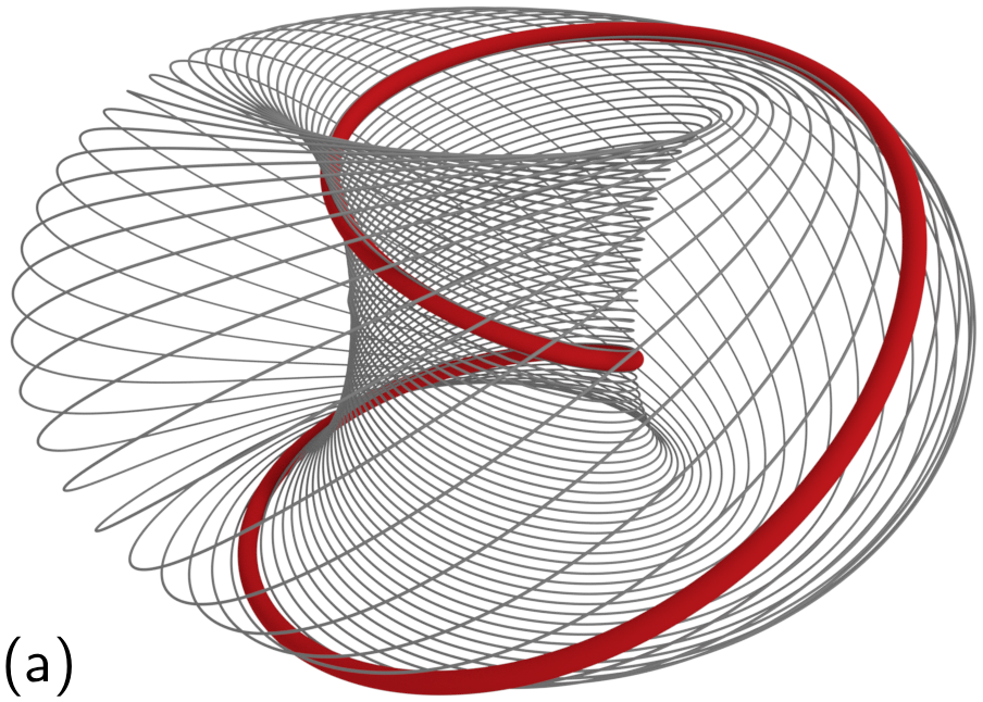
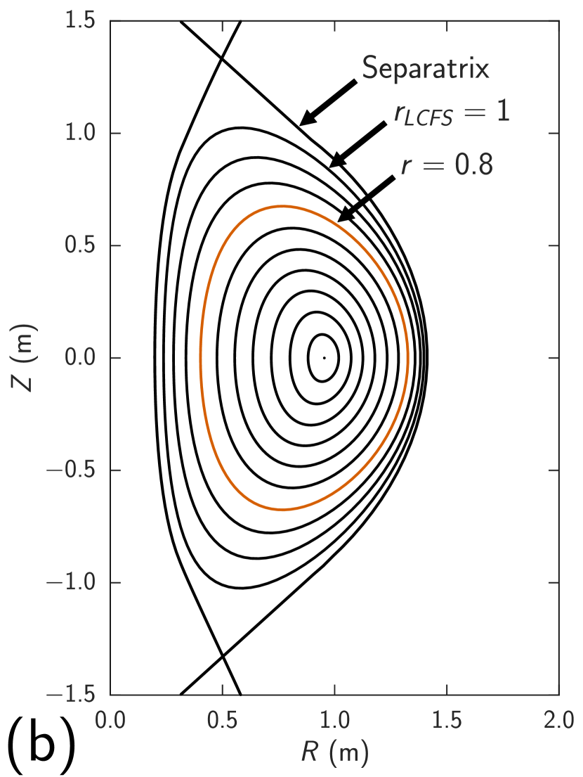
A GS2 flux tube is a twisted box of finite radial and poloidal width that follows a magnetic field line once around the tokamak in the poloidal direction (figure 1(a)). We assume that the underlying equilibrium is axisymmetric, so a single flux tube can be used to simulate the entire flux surface, allowing a large saving in computational cost. In this local approach, all equilibrium gradients (of density, velocity, and temperature) are assumed constant across the radial extent of the flux tube. We pick the time s from the beginning of the discharge and the radial location , where is the diameter of the flux surface hosting our flux tube, at the height of the magnetic axis, and is the diameter of the last closed flux surface (the “edge” of the plasma). This definition of the radial location is convenient because it coincides with the Miller et al. (1998) parametrisation of the flux tube geometry used by GS2. Figure 1(b) shows a poloidal projection of the MAST flux surfaces for discharge #27268 with the flux surface at highlighted.
The gyrokinetic equation (Frieman & Chen 1982; see appendix A) solved by GS2 gives us the time evolution of the perturbed distribution function of particles of species (ions or electrons), where is the spatial position and the velocity. Gyrokinetic theory makes use of the fact that turbulent fluctuations in a tokamak plasma occur at much longer time scales than the Larmor motion of the particles (although still much shorter than the evolution of the background thermal and magnetic equilibrium state). This allows the Larmor motion to be averaged over analytically, leading to a kinetics of Larmor rings, whose distribution depends on two, rather than three velocity variables (parallel and perpendicular velocities, but not the gyroangle), reducing the phase space from six to five dimensions — a more tractable problem than the Vlasov–Boltzmann equation for the evolution of the full distribution function.
3 Turbulent heat flux
With the knowledge of the distribution function, one can calculate any characteristics of the turbulence. In particular, the turbulent heat flux as a function of the temperature gradient, flow shear, or any other equilibrium parameters is a key quantity of interest. Focusing on the heat flux will allow us to diagnose the transition to turbulence, as values greater than zero indicate a turbulent state. We focus here on the heat flux due to the ions (deuterium in our simulations). The radially outward, time-averaged ion heat (energy) flux through a volume enveloping a given flux surface is
| (1) |
where is the drift velocity due to the perturbed electric field, calculated from via the plasma quasineutrality constraint (see appendix A), and indicates an average in time. is typically normalised by the so-called gyro-Bohm value, , where , , and are the ion density, temperature, and Larmor radius, respectively (it is a feature of the asymptotic ordering on which the gyrokinetic theory is based that is a finite number; see Abel et al. 2013).
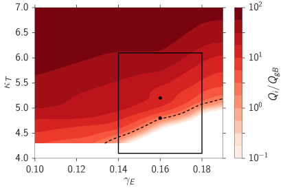
To map out the transition to turbulence in our system, we vary the flow shear and the temperature gradient around their experimental values ( and ), and covering the range and . Figure 2 shows the turbulent heat flux in a part of this range, close to the threshold. All simulations were run until they reached a statistically steady state, i.e., until the running time average value became independent of time. An average was then taken over a period of (which represents s) during this steady state. Examining both the range of values of compatible with experiment and the experimentally determined value (Field et al., 2014), we see that the turbulent state found in a real device is close to the threshold (perhaps not a surprising conclusion, but an important one to be able to make quantitatively). Experimental investigations (e.g., Mantica et al. 2009) corroborate this observation for other tokamaks and show that the proximity to threshold is enforced by the rapid increase in as the stability parameter is increased from its critical value (“stiff transport”). A similar conclusion can be drawn from figure 2: small increases in lead to order-of-magnitude changes in . We find that very small departures of the flow shear from the threshold also lead to large increases of , showing that flow shear matters at experimentally relevant values and heat transport is highly sensitive to it.
4 Subcritical turbulence
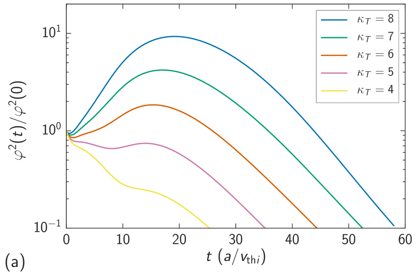
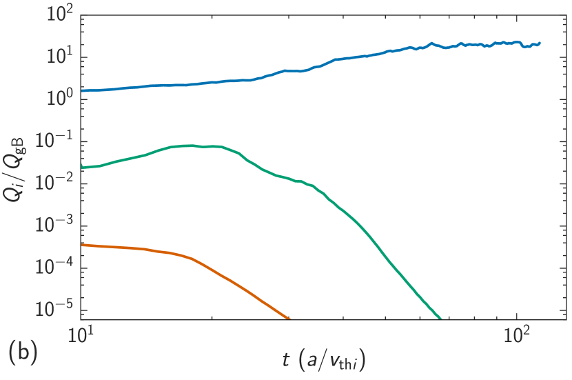
Usually one would also carry out a sequence of linear simulations to ascertain whether the turbulence threshold found nonlinearly coincides with the linear stability boundary. Doing these simulations showed that all modes in our system at all parameter values that we have investigated (except ) were formally linearly stable. Initial perturbations did, however, exhibit transient growth, typically for a longer period in the cases far from the nonlinear threshold, as illustrated in figure 3(a) (cf. Newton et al. 2010; Highcock et al. 2010; Barnes et al. 2011a; Schekochihin et al. 2012; Highcock et al. 2012). Nonlinearly, this means that, beyond a certain threshold in and , and given a large enough initial perturbation, subcritical turbulence can be sustained.222Note in figure 3(a) that the turbulence threshold corresponds roughly to the values of the stability parameters and at which the transient amplification factor drops below unity (cf. Highcock et al. 2012). This is illustrated in figure 3(b), showing the effect of changing the initial perturbation amplitude. There is clearly a critical amplitude above which the nonlinearity can pick up the transiently amplified perturbations (very weakly amplified, when close to threshold) and give rise to a non-zero saturated state. Importantly, the saturation level does not depend on the size of the initial perturbation (as long as the latter is large enough). Thus, in the experimental instance that we have considered, ion-scale turbulence in MAST in the presence of flow shear is subcritical and so tokamak plasmas join a plethora of neutral fluid systems where the transition to turbulence depends strongly on the (size of) initial perturbation (Trefethen et al., 1993; Darbyshire & Mullin, 1995): e.g., both Poiseuille and Couette flows are formally stable (Salwen et al., 1980; Trefethen et al., 1993), but still able to transition to a nonlinear, turbulent state; a similar situation arises in Keplerian shear flows believed to exist in accretion disks (Riols et al., 2013). Recent theoretical work, involving very simple models, suggested that this may also be possible in plasmas (Newton et al., 2010; Schekochihin et al., 2012; Landreman et al., 2015), as did simulations of simplified tokamak equilibria (Barnes et al., 2011a; Highcock et al., 2010, 2011, 2012), but ours appears to be the first demonstration of subcritical ion-scale turbulence in a specific, experimentally diagnosed tokamak plasma.
5 Scenario for transition to turbulence
How does the transition to subcritical turbulence occur, i.e., what sequence of turbulent states does the system go through as either or crosses the critical threshold and moves away from it into ever more strongly driven regimes? It is clear that the transition cannot occur via near-threshold states featuring arbitrarily small fluctuations everywhere, because sustaining subcritical turbulence requires finite initial perturbations. These initial perturbations must be larger near the threshold than far from it because the amount of amplification expected during transient growth tends to decrease close to the threshold (Schekochihin et al., 2012; Highcock et al., 2012). If the typical maximum amplitude of the fluctuations in the saturated state must remain finite, one way to reduce the turbulent heat flux to low values near the threshold is by reducing the fraction of the system’s volume taken up by turbulence, i.e., by concentrating intense fluctuations in a shrinking part of space. This is precisely what happens, as we will now demonstrate.
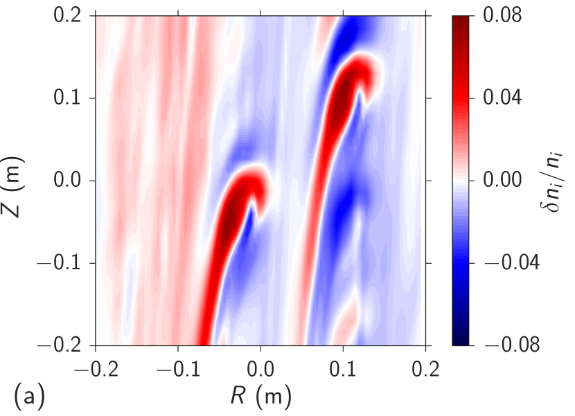
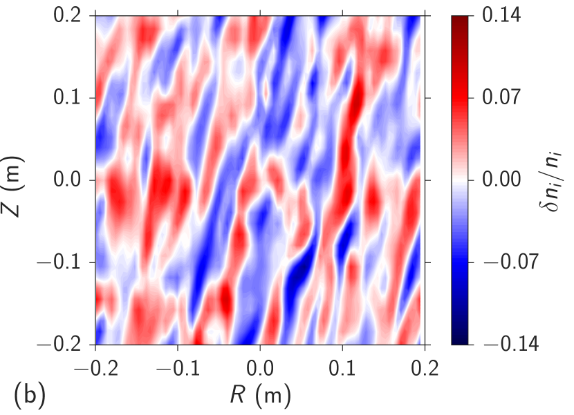
In figure 4, we show real-space snapshots of the turbulent density-fluctuation field in the poloidal cross section of our flux tube at and for two different temperature gradients: , which is very close to the threshold, and , a case that represents more strongly driven turbulence away from the threshold (both points are within the experimentally consistent range; see figure 2). We find that the near-threshold turbulent state is dominated by long-lived, intense coherent structures, which travel across the domain both radially and poloidally, whereas far from the threshold, we observe a more conventional chaotic turbulent state characterised by interacting eddies. These two cases are representative of the relevant regions of our parameter space. We always find that long-lived, large-amplitude structures form in the near-threshold cases and survive against the background of very weak ambient fluctuations. As the system is taken away from the threshold by increasing or decreasing , these structures become more numerous (i.e., more volume-filling) while retaining comparable amplitude, eventually start interacting with each other, and break up. Finally, far from the threshold, we observe no discernible long-lived structures, but rather strong time-variable fluctuations everywhere with amplitudes that increase with or decreasing .
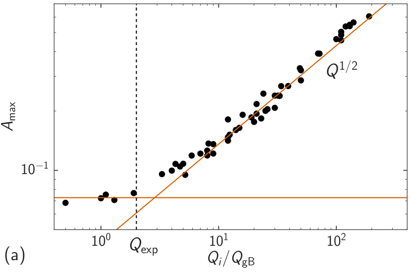
Let us make the statements above more quantitative. Consider how the maximum amplitude of the density perturbations found across the domain (and averaged over time) changes as our stability parameters and change. Since is a strong function of both and , we can measure the “distance from threshold” by just using as a stability parameter. A naive estimate based on (1) is
| (2) |
where (which in the gyrokinetic theory is an order-unity quantity; see Abel et al. 2013). We have estimated the radial velocity as , where is the typical poloidal wave number ( in this regime) of the fluctuations of the electrostatic potential , which are related (by order of magnitude) to the electron (and, therefore, ion) density via the Boltzmann response . Figure 5(a) shows the relationship between and for a number of simulations with different values of and . While the naive scaling (2) is indeed manifest far from the threshold, it is a striking feature of figure 5(a) that the maximum fluctuation amplitude hits a finite “floor” as decreases to and below its experimental value — this coincides with the appearance of long-lived structures illustrated in figure 4(a). Thus, while in the conventional supercritical turbulence, we might have observed smaller fluctuation amplitudes corresponding to lower heat fluxes all the way to the threshold, in the present subcritical turbulent system, we see the heat flux decrease while the maximum fluctuation amplitude remains constant.
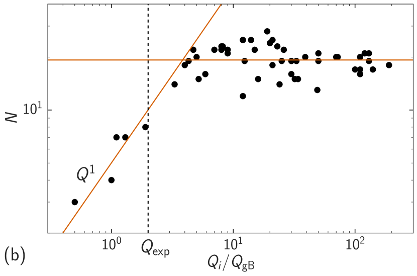
As we argued above, it does this via reduction of the volume taken up by large fluctuations. We will now show this by measuring the typical number of the turbulent structures as a function of distance to threshold. While 2D structures are easily discerned by a human eye (e.g., in figure 4(a), there are two), counting them systematically is a not entirely trivial problem, which is often encountered in computer-vision and pattern-recognition applications. It has been considered before in the context of experimental measurements of turbulence (Kauschke 1999; Müller et al. 2005; see review of various techniques by Love & Kamath 2007). Structure counting can be reduced to an image-labelling, or segmentation, problem by applying a threshold function to our density fluctuations: setting values below a certain percentile (here 75%) of the maximum amplitude to 0 and above it to 1. We are then left with an array of 1’s representing our structures against a background of 0’s. We employ a general-purpose image processing package scikit-image (van der Walt et al., 2014), which implements an efficient labelling algorithm (Fiorio & Gustedt, 1996), to label connected regions, i.e., turbulent structures. In order to improve the reliability of the labelling algorithm, we applied a Gaussian image filter (with a standard deviation on the order of the grid scale) as a pre-processing step and also removed structures below 10% of the mean structure size as a post-processing step. These steps are justified because we are hunting intense, relatively large-scale structures.
Figure 5(b) shows the results of the above analysis: the number of turbulent structures with amplitudes above the 75th percentile versus the heat flux. As in figure 5(a), there are two distinct regimes: grows with until the structures have filled the simulation domain (which happens just beyond the experimental value of the flux), whereupon tends to a constant. Taking figures 5(a) and 5(b) in combination, we have, roughly, , i.e., near the threshold, turbulent heat flux increases because coherent structures become more numerous (but not more intense: grows, stays constant), whereas far from the threshold, it does so because the fluctuation amplitude increases (while stays constant).
6 Conclusion
In conclusion, we have discovered, using numerical simulations of an experimentally relevant fusion plasma, a novel scenario for transition to turbulent state — which applies when the turbulence is subcritical. Above a certain critical value of and below a critical value of , a large enough initial perturbation will ignite turbulence. Near the threshold, the density and temperature fluctuations (and hence heat flux) are concentrated in long-lived, intense coherent structures (interestingly, this is reminiscent of the transition via localised patches in pipe flows; see Barkley et al. 2015, or transition to MRI turbulence in Keplerian accretion flows; see Riols et al. 2016, 2013). As the stability parameters depart slightly from their critical values into the more strongly driven regime, the number of these structures increases rapidly while their amplitude stays roughly constant (in contrast to the conventional supercritical turbulence, where the amplitude increases with because arbitrarily low-amplitude turbulence can be supported close to threshold). Increasing the turbulent drive further leads to the turbulent structures filling the simulation domain and any further increase in the heat flux is caused by an increase in turbulent amplitude. The latter regime is similar to the conventional plasma turbulence.
It is the presence of flow shear that appears to be the key feature that allows tokamak turbulence to exist in two distinct regimes — more strictly speaking, these are two regimes of anomalous transport, rather than turbulence: it is not obvious that the structure-dominated near-threshold state can be viewed as properly turbulent, representing perhaps a persistent nonlinear solution rather than full-scale chaos (cf. Riols et al. 2016). It will be very interesting to see if a structure-dominated regime can be detected in MAST or in other tokamaks where significant flow shear is present: so far, there are some tentative but encouraging indications that such a regime might manifest itself in experimentally observed skewed probability distributions of density fluctuations (Fox et al., 2016).
The new regime of tokamak turbulence described above, besides raising interesting questions of theory of the subcritical transition and its degree of universality, also raises potentially useful ones regarding ways (e.g., optimal combinations of momentum and power input) in which such a turbulence could be controlled and the associated heat flux further reduced, leading to better confined plasmas.
Acknowledgements
We would like to thank M. Barnes, J. Ball, G. Colyer, M. Fox and F. Parra for many useful discussions. The simulations were carried out in part using the HELIOS supercomputer system at International Fusion Energy Research Centre, Aomori, Japan, under the Broader Approach collaboration between Euratom and Japan, implemented by Fusion for Energy and JAEA. Simulations carried out using the ARCHER UK National Supercomputing Service (http://www.archer.ac.uk) were provided by the Plasma HEC Consortium (EP/L000237/1) and the Collaborative Computational Project in Plasma Physics funded by UK EPSRC (EP/M022463/1). This work has been carried out within the framework of the EUROfusion Consortium and received funding from the European Union’s Horizon 2020 research and innovation programme and Euratom research and training programme 2014-2018 under grant agreement number 633053. The views and opinions expressed herein do not necessarily reflect those of the European Commission. The work of A. A. S. was supported in part by grants from UK EPSRC and STFC.
Appendix A Gyrokinetic model and numerical set up
Here we outline the theoretical framework that we have used for modelling plasma turbulence and give all the information necessary to reproduce our GS2 simulations.
The gyrokinetic equation (Frieman & Chen, 1982; Abel et al., 2013) describes the time evolution of the perturbed (from a background Maxwellian ) distribution function of particles of species . Here we solve an approximate form of this equation arising from assuming, formally, that the Mach number of the plasma rotational flow is small, but that the flow shear is large enough to matter: namely, if is the angular frequency of toroidal rotation, then
| (3) |
where is the major radius of the toroidal device at the location of our flux tube. This ordering allows one to formulate local gyrokinetics in a rotating flux surface, neglecting such effects as Coriolis and centrifugal forces, but retaining flow shear. With this ordering and assuming also purely electrostatic perturbations (no fluctuating magnetic fields), the gyrokinetic system of equations is written as follows (see §11 of Abel et al. 2013 or appendix A of Schekochihin et al. 2012). The perturbed distribution function is split into a part corresponding to Boltzmann density response and the distribution of the gyrocentres:
| (4) |
where , , , are the charge, mass, density, and temperature of particles of species , is the electrostatic potential perturbation, is the position of the centre of a particle’s Larmor orbit, is the position of the particle, is a unit vector in the direction of the magnetic field , is the velocity of the particle perpendicular to the magnetic field, is the cyclotron frequency, is the speed of light, the particle energy, its magnetic moment and the sign of its parallel velocity (, and are the velocity-space variables used by the GS2 code); the velocities are taken in the frame rotating with the angular frequency , which, like and , is a function of the poloidal flux only. The evolution equation for is then
| (5) |
where , with being the toroidal angle, is the toroidal rotation velocity,
| (6) |
is the magnetic drift velocity,
| (7) |
is the drift velocity, is an average over a particle orbit at constant guiding-centre position , is the linearised collision operator, is the toroidal component of the magnetic field. To calculate in (5), the quasineutrality condition is used:
| (8) |
where means a gyroaverage at constant .
The last term in (5) represents the advection by the gyroaveraged velocity of the Maxwellian plasma equilibrium distribution characterised by , and . These are functions only of the flux surface, conventionally labelled by the poloidal flux , but here this dependence has been converted to the Miller et al. (1998) radial coordinate , where is the diameter of the flux surface of interest at the elevation of the magnetic axis and is the diameter of the last closed flux surface (see figure 1(b)). Since is also a flux-surface label, . The gradients that appear in the right-hand side of (5) are sources of free energy in the plasma. In local flux-tube calculations, these are approximated as constant parameters and the following definitions for them are introduced:
| (9) |
where is the “safety factor”. Since this quantity in a tokamak is, approximately, , where is the poloidal component of the magnetic field, has the meaning of the (non-dimensionalised) part of the toroidal flow shear that is perpendicular to the local magnetic field. The special relevance of this quantity becomes obvious if we “unpack” what is meant by in the left-hand side of (5). Since GS2 solves the gyrokinetic equation locally in the vicinity of a particular flux surface , we may expand, inside our flux tube, , where is the distance from the flux surface. Then333This is obtained using the representation of the axisymmetric magnetic field in a torus. Note that only needs to be expanded because we assumed in (3) that it changes on a scale smaller than (which is the scale length of change of geometrical and magnetic quantities such as or ).
| (10) |
where is the unit vector in the direction perpendicular to the field line but tangent to the flux surface. If we now go to the frame rotating with the flux surface at the rate and also use the fact that, in gyrokinetics, gradients parallel to are always small compared to those perpendicular to it, we find
| (11) |
with as defined in (9). The prefactor enclosed in the parentheses is close to unity and so is the non-dimensionalised flow shear that operates on the distribution function. There is also free-energy injection associated with the presence of the flow shear, as is manifest in the presence of a term proportional to on the right-hand side of (5), but, at the values of considered here, the (destabilising) effect of this term, while included in our simulations, is irrelevant in comparison with that of the ion-temperature gradient (see Schekochihin et al. 2012 for further details on this).
GS2 solves the GK equations (5) and (8) in a flux tube following the flux surface once around the torus poloidally (see figure 1(a) and discussion in the main text). Figure 1(b) shows the poloidal projection of the MAST flux surfaces with the flux surface at marked. The marked flux surface is the location at which we solve the GK equation. It can be described as located in the outer core of the device.
Each GS2 simulation requires input of a number of constant parameters that define the magnetic-field geometry (e.g., elongation of the flux surface, its triangularity, magnetic shear, etc.), the properties of the mix of the participating particle species (their masses, charges, densities, temperatures, collisionalities, etc.) and the local thermal equilibrium properties of the plasma — in particular, the gradients defined in (9). The use of the local formulation of gyrokinetics requires that . At the radial location considered in this paper, m and the minor radius m, which implies and justifies the local approximation of gyrokinetics that we have used. Table 1 gives a list of the equilibrium parameters, which have been determined via diagnostic measurements of the MAST discharge #27268 (at s). In particular, and were obtained from charge-exchange-recombination spectroscopy measurements (Conway et al., 2006) and and were obtained from a Thomson scattering diagnostic (Scannell et al., 2010). The magnetic geometry in our simulations is described by the Miller et al. (1998) parametrisation and the geometric parameters were obtained from an EFIT reconstruction (Lao et al., 1985) of the equilibrium. All these parameters were fixed at the same values in all our simulations, except the ion temperature gradient and the flow shear (their experimental values are and ; see figure 2 for error bars on these values).
The resolution of our simulations (with corresponding GS2 input parameters) was as follows: 128 radial modes (nx), 96 binormal modes (ny), 20 parallel grid points (ntheta), 16 energy grid points (negrid), and 27 pitch-angle grid points (). The box sizes were approximately ( and ) and () in the radial and binormal directions, respectively, and in the parallel direction, given that GS2 uses the poloidal angle as the parallel coordinate.
| Name | GS2 variable | Value |
| beta | 0.0047 | |
| beta_prime_input | -0.12 | |
| Effective ion charge | zeff | 1.59 |
| Electron collisionality | vnewk_2 | 0.59 |
| Electron density | dens_2 | 1.00 |
| Electron density gradient | fprim_2 | 2.64 |
| Electron mass | mass_2 | |
| Electron temperature | temp_2 | 1.09 |
| Electron temperature gradient | tprim_2 | 5.77 |
| Elongation | akappa | 1.46 |
| Elongation derivative | akappri | 0.45 |
| Flow shear | g_exb | [0, 0.19] |
| Ion collisionality | vnewk_1 | 0.02 |
| Ion density , | dens_1 | 1.00 |
| Ion density gradient | fprim_1 | 2.64 |
| Ion mass , | mass_1 | 1.00 |
| Ion temperature , | temp_1 | 1.00 |
| Ion temperature gradient | tprim_1 | [4.3, 8.0] |
| Magnetic shear | s_hat_input | 4.00 |
| Magnetic field reference point | r_geo | 1.64 |
| Major radius | rmaj | 1.49 |
| Miller radial coordinate | rhoc | 0.80 |
| Safety factor | qinp | 2.31 |
| Shafranov Shift | shift | -0.31 |
| Triangularity | tri | 0.21 |
| Triangularity derivative | tripri | 0.46 |
References
- Abel et al. (2013) Abel, I. G., Plunk, G. G., Wang, E., Barnes, M., Cowley, S. C., Dorland, W. & Schekochihin, A. A. 2013 Multiscale gyrokinetics for rotating tokamak plasmas: fluctuations, transport and energy flows. Rep. Prog. Phys. 76, 116201.
- Baker et al. (2001) Baker, D. R., Greenfield, C. M., Burrell, K. H., DeBoo, J. C., Doyle, E. J., Groebner, R. J., Luce, T. C., Petty, C. C., Stallard, B. W., Thomas, D. M. & Wade, M. R. 2001 Thermal diffusivities in DIII-D show evidence of critical gradients. Phys. Plasmas 8, 4128.
- Barkley et al. (2015) Barkley, D., Song, B., Mukund, V., Lemoult, G., Avila, M. & Hof, B. 2015 The rise of fully turbulent flow. Nature 526, 550.
- Barnes et al. (2011a) Barnes, M., Parra, F. I., Highcock, E. G., Schekochihin, A. A., Cowley, S. C. & Roach, C. M. 2011a Turbulent transport in tokamak plasmas with rotational shear. Phys. Rev. Lett. 106, 175004.
- Barnes et al. (2011b) Barnes, M., Parra, F. I. & Schekochihin, A. A. 2011b Critically balanced ion temperature gradient turbulence in fusion plasmas. Phys. Rev. Lett. 107, 115003.
- Burin et al. (2005) Burin, M. J., Tynan, G. R., Antar, G. Y., Crocker, N. A. & Holland, C. 2005 On the transition to drift turbulence in a magnetized plasma column. Phys. Plasmas 12, 052320.
- Burrell (1997) Burrell, K. H. 1997 Effects of ExB velocity shear and magnetic shear on turbulence and transport in magnetic confinement devices. Phys. Plasmas 4, 1499.
- Conway et al. (2006) Conway, N. J., Carolan, P. G., McCone, J., Walsh, M. J. & Wisse, M. 2006 High-throughput charge exchange recombination spectroscopy system on MAST. Rev. Sci. Instrum. 77, 10F131.
- Coppi et al. (1967) Coppi, B., Rosenbluth, M. N. & Sagdeev, R. Z. 1967 Instabilities due to temperature gradients in complex magnetic field configurations. Phys. Fluids 10, 582.
- Darbyshire & Mullin (1995) Darbyshire, A. G. & Mullin, T. 1995 Transition to turbulence in constant-mass-flux pipe flow. J. Fluid Mech. 289, 83.
- Dimits et al. (2000) Dimits, A. M., Bateman, G., Beer, M. A., Cohen, B. I., Dorland, W., Hammett, G. W., Kim, C., Kinsey, J. E., Kotschenreuther, M., Kritz, A. H., Lao, L. L., Mandrekas, J., Nevins, W. M., Parker, S. E., Redd, A. J., Shumaker, D. E., Sydora, R. & Weiland, J. 2000 Comparisons and physics basis of tokamak transport models and turbulence simulations. Phys. Plasmas 7, 969.
- Fasoli et al. (2016) Fasoli, A., Brunner, S., Cooper, W. A., Graves, J. P., Ricci, P., Sauter, O. & Villard, L. 2016 Computational challenges in magnetic-confinement fusion physics. Nature Phys. 12, 411.
- Field et al. (2014) Field, A. R., Dunai, D., Ghim, Y.-c., Hill, P., McMillan, B. F., Roach, C. M., Saarelma, S, Schekochihin, A. A. & Zoletnik, S. 2014 Comparison of BES measurements of ion-scale turbulence with direct gyro-kinetic simulations of MAST L-mode plasmas. Plasma Phys. Control. Fusion 56, 025012.
- Field et al. (2011) Field, A. R., Michael, C., Akers, R.J., Candy, J., Colyer, G., Guttenfelder, W., Ghim, Y.-c., Roach, C.M. & Saarelma, S. 2011 Plasma rotation and transport in MAST spherical tokamak. Nucl. Fusion 51, 063006.
- Fiorio & Gustedt (1996) Fiorio, C. & Gustedt, J. 1996 Two linear time Union-Find strategies for image processing. Theor. Comput. Sci. 154, 165.
- Fox et al. (2016) Fox, M. F. J., van Wyk, F., Field, A. R., Ghim, Y.-c., Parra, F. I. & Schekochihin, A. A. 2016 Symmetry breaking in MAST plasma turbulence due to toroidal flow shear, arXiv: 1609.08981.
- Frieman & Chen (1982) Frieman, E. A. & Chen, L. 1982 Nonlinear gyrokinetic equations for low-frequency electromagnetic waves in general plasma equilibria. Phys. Fluids 25, 502.
- Ghim et al. (2014) Ghim, Y.-c., Field, A. R., Schekochihin, A. A., Highcock, E. G., Michael, C. & the MAST Team 2014 Local dependence of ion temperature gradient on magnetic configuration, rotational shear and turbulent heat flux in MAST. Nucl. Fusion 54, 042003.
- Highcock et al. (2011) Highcock, E. G., Barnes, M., Parra, F. I., Schekochihin, A. A., Roach, C. M. & Cowley, S. C. 2011 Transport bifurcation induced by sheared toroidal flow in tokamak plasmas. Phys. Plasmas 18, 102304.
- Highcock et al. (2010) Highcock, E. G., Barnes, M., Schekochihin, A. A., Parra, F. I., Roach, C. M. & Cowley, S. C. 2010 Transport bifurcation in a rotating tokamak plasma. Phys. Rev. Lett. 105, 215003.
- Highcock et al. (2012) Highcock, E. G., Schekochihin, A. A., Cowley, S. C., Barnes, M., Parra, F. I., Roach, C. M. & Dorland, W. 2012 Zero-turbulence manifold in a toroidal plasma. Phys. Rev. Lett. 109, 265001.
- Kauschke (1999) Kauschke, U. 1999 Observation of coherent self-organized drift structures in a turbulent DC discharge. Plasma Phys. Control. Fusion 35, 93.
- Klinger et al. (1997) Klinger, T., Latten, A., Piel, A., Bonhomme, G. & Pierre, T. 1997 Route to drift wave chaos and turbulence in a bounded low-beta plasma experiment. Phys. Rev. Lett. 79, 3913.
- Kotschenreuther et al. (1995) Kotschenreuther, M., Dorland, W., Beer, M. A. & Hammett, G. W. 1995 Quantitative predictions of tokamak energy confinement from first-principles simulations with kinetic effects. Phys. Plasmas 2, 2381.
- Krushelnick & Cowley (2005) Krushelnick, K. & Cowley, S. 2005 Reduced turbulence and new opportunities for fusion. Science 309, 1502.
- Landreman et al. (2015) Landreman, M., Plunk, G. G. & Dorland, W. 2015 Generalized universal instability: transient linear amplification and subcritical turbulence. J. Plasma Phys. 81, 905810501.
- Lao et al. (1985) Lao, L.L., John, H. St., Stambaugh, R.D., Kellman, A.G. & Pfeiffer, W. 1985 Reconstruction of current profile parameters and plasma shapes in tokamaks. Nucl. Fusion 25, 1611.
- Love & Kamath (2007) Love, N. S. & Kamath, C. 2007 Image analysis for the identification of coherent structures in plasma. In Proc. SPIE, 1, vol. 6696, p. 66960D.
- Mantica et al. (2009) Mantica, P., Strintzi, D., Tala, T., Giroud, C., Johnson, T., Leggate, H., Lerche, E., Loarer, T., Peeters, A. G., Salmi, A., Sharapov, S., Van Eester, D., De Vries, P. C., Zabeo, L. & Zastrow, K.-D. 2009 Experimental study of the ion critical-gradient length and stiffness level and the impact of rotation in the JET Tokamak. Phys. Rev. Lett. 102, 1.
- Miller et al. (1998) Miller, R. L., Chu, M. S., Greene, J. M., Lin-Liu, Y. R. & Waltz, R. E. 1998 Noncircular, finite aspect ratio, local equilibrium model. Phys. Plasmas 5, 973.
- Müller et al. (2005) Müller, S. H., Fasoli, A., Labit, B., McGrath, M., Pisaturo, O., Plyushchev, G., Podestà, M. & Poli, F. M. 2005 Basic turbulence studies on TORPEX and challenges in the theory-experiment comparison. Phys. Plasmas 12, 090906.
- Newton et al. (2010) Newton, S. L., Cowley, S. C. & Loureiro, N. F. 2010 Understanding the effect of sheared flow on microinstabilities. Plasma Phys. Control. Fusion 52, 125001.
- Reynolds (1883) Reynolds, O. 1883 An experimental investigation of the circumstances which determine whether the motion of water shall be direct or sinuous, and of the law of resistance in parallel channels. Phil. Trans. R. Soc. Lond. 174, 935.
- Riccardi et al. (1997) Riccardi, C., Xuantong, D., Salierno, M., Gamberale, L. & Fontanesi, M. 1997 Experimental analysis of drift waves destabilization in a toroidal plasma. Phys. Plasmas 4, 3749.
- Riols et al. (2013) Riols, A, Rincon, F, Cossu, C, Lesur, G, Longaretti, P.-Y., Ogilvie, G I & Herault, J 2013 Global bifurcations to subcritical magnetorotational dynamo action in Keplerian shear flow. J. Fluid Mech. 731, 1.
- Riols et al. (2016) Riols, A., Rincon, F., Cossu, C., Lesur, G., Ogilvie, G. I. & Longaretti, P-Y. 2016 Magnetorotational dynamo chimeras. The missing link to turbulent accretion disk dynamo models?, arXiv: 1607.02903.
- Roach et al. (2009) Roach, C. M., Abel, I. G., Akers, R. J., Arter, W., Barnes, M., Camenen, Y., Casson, F. J., Colyer, G., Connor, J. W., Cowley, S. C., Dickinson, D., Dorland, W. D., Field, A. R., Guttenfelder, W., Hammett, G. W., Hastie, R., Highcock, E. G., Loureiro, N. F., Peeters, A. G., Reshko, M., Saarelma, S., Schekochihin, A. A., Valovic, M. & Wilson, H. R. 2009 Gyrokinetic simulations of spherical tokamaks. Plasma Phys. Control. Fusion 51, 124020.
- Salwen et al. (1980) Salwen, H., Cotton, F. W. & Grosch, C. E. 1980 Linear stability of Poiseuille flow in a circular pipe. J. Fluid Mech. 98, 273.
- Scannell et al. (2010) Scannell, R., Walsh, M. J., Dunstan, M. R., Figueiredo, J., Naylor, G., O’Gorman, T., Shibaev, S., Gibson, K. J. & Wilson, H. 2010 A 130 point Nd:YAG Thomson scattering diagnostic on MAST. Rev. Sci. Instrum. 81, 10D520.
- Schekochihin et al. (2012) Schekochihin, A. A., Highcock, E. G. & Cowley, S. C. 2012 Subcritical fluctuations and suppression of turbulence in differentially rotating gyrokinetic plasmas. Plasma Phys. Control. Fusion 54, 055011.
- Trefethen et al. (1993) Trefethen, L. N., Trefethen, A. E., Reddy, S. C. & Driscoll, T. A. 1993 Hydrodynamic stability without eigenvalues. Science 261, 578.
- van der Walt et al. (2014) van der Walt, S., Schönberger, J. L., Nunez-Iglesias, J., Boulogne, F., Warner, J. D., Yager, N., Gouillart, E., Yu, T. & the scikit-image contributors 2014 scikit-image: image processing in Python. PeerJ 2, e453.
- Weixing et al. (1993) Weixing, Ding, Huang Wei, Wang Xiaodong & Yu, C. X. 1993 Quasiperiodic transition to chaos in a plasma. Phys. Rev. Lett. 70, 170.