Formation of X-ray emitting stationary shocks in magnetized protostellar jets

Abstract

Context. X-ray observations of protostellar jets show evidence of strong shocks heating the plasma up to temperatures of a few million degrees. In some cases, the shocked features appear to be stationary. They are interpreted as shock diamonds.

Aims. We aim at investigating the physics that guides the formation of X-ray emitting stationary shocks in protostellar jets, the role of the magnetic field in determining the location, stability, and detectability in X-rays of these shocks, and the physical properties of the shocked plasma.

Methods. We performed a set of 2.5-dimensional magnetohydrodynamic numerical simulations modelling supersonic jets ramming into a magnetized medium and explored different configurations of the magnetic field. The model takes into account the most relevant physical effects, namely thermal conduction and radiative losses. We compared the model results with observations, via the emission measure and the X-ray luminosity synthesized from the simulations.

Results. Our model explains the formation of X-ray emitting stationary shocks in a natural way. The magnetic field collimates the plasma at the base of the jet and forms there a magnetic nozzle. After an initial transient, the nozzle leads to the formation of a shock diamond at its exit which is stationary over the time covered by the simulations ($\sim 40-60$ yr; comparable with time scales of the observations). The shock generates a point-like X-ray source located close to the base of the jet with luminosity comparable with that inferred from X-ray observations of protostellar jets. For the range of parameters explored, the evolution of the post-shock plasma is dominated by the radiative cooling, whereas the thermal conduction slightly affects the structure of the shock.

1 Introduction

The early stages of a star birth are characterized by a variety of mass ejection phenomena, including outflows and collimated jets that are strongly related with the accretion process developed in the context of the star-disc interaction. In fact, magnetohydrodynamic (MHD) centrifugal models for jet launching (Blandford & Payne, 1982; Pudritz & Norman, 1983) indicated that protostellar jets could provide a valid solution to the angular momentum problem (see Bacciotti et al. 2002 for a wider description) via vertical transport along the ordered component of the strong magnetic field threading the disk. According to the widely accepted magneto-centrifugal launching scenario (Ferreira et al., 2006; Gomez de Castro & Pudritz, 1993), outflows in young stars are driven from the inner portion of accretion discs and dense plasma from the disc is collimated into jets. This scenario was challenged by several models based on different lines of evidence from the observations suggesting the presence of dust in jets due to material from the outer part of the disc (Podio et al., 2009). Thus several MHD ejection sites probably coexist in young stars, and the difficulty is to determine the relative contribution of each to the observed jet (for a complete review confronting observations and theory see Frank et al. 2014).

The general consensus is that magnetic fields play a fundamental role in launching, collimating and stabilizing the plasma of jets. This idea was recently corroborated by scaled laboratory experiments that are representative of young stellar object outflows (Albertazzi et al., 2014). These experiments revealed that stable and narrow collimation of the entire flow can result from the presence of a poloidal magnetic field. A key observational diagnostic to discriminate between different theories could be the detection of possible signatures of rotation in protostellar jets. Pushing the limits of observational resolution, several authors described the detection of asymmetric Doppler shifts in emission lines from opposite borders of the flow in different objects (Bacciotti et al., 2002; Woitas et al., 2005; Coffey et al., 2004, 2007, 2015). However, this possibility is still undergoing active debate. For example, some inconsistencies in rotation signatures were found at different positions along the jet in a UV study of RW Aur (Coffey et al., 2012) and in a near-infrared study of DG Tau (White et al., 2014) where systematic transverse velocity gradients could not be identified. Alternative interpretations include asymmetric shocking and/or jet precession (e.g., Soker, 2005; Cerqueira et al., 2006; Correia et al., 2009).

Usually jets from young stars are revealed by the presence of a chain of knots, forming the so-called Herbig-Haro (HH) objects. The observations of multiple HH objects showed a knotty structure along the jet axis interpreted as the consequence of the pulsing nature of the ejection of material by the star (e.g. Raga et al. 1990, 2007; Bonito et al. 2010a, b; and references therein). After been ejected, the trains of blobs forming the jet move through the ambient medium and they may interact and produce shocks and complex structures that are observed at different wavelengths. In particular, observations showed evidence of faint X-ray emitting sources forming within the jet (e.g. Pravdo et al. 2001; Favata et al. 2002; Bally et al. 2003; Pravdo et al. 2004; Tsujimoto et al. 2004; Güdel et al. 2005; Stelzer et al. 2009). The origin of this X-ray emission was investigated through hydrodynamic models which have shown that the observations are consistent with the production of strong shocks that heat the plasma up to temperatures of a few million degrees (Bonito et al., 2007, 2010a, 2010b).

In some cases, the shocked features appeared to be stationary and located close to the base of the jet (e.g. HH154, Favata et al. 2006; DG Tau, Güdel et al. 2005). In one of the best-studied X-ray jet, HH154, the X-ray emission consisted of a bright stationary component and a fainter and slightly variable elongated component (see Favata et al., 2006). On the base of hydrodynamic modelling, this source was interpreted as a shock diamond formed just after a nozzle from which the jet originated (Bonito et al., 2011). This scenario was recently supported by scaled laboratory experiments showing the formation of a shock at the base of a laboratory jet that may explain the X-ray emission features observed at the base of some protostellar jets (Albertazzi et al., 2014).

Previous MHD models of protostellar jets were aimed at studying the effect of the magnetic field on the dynamical evolution of HH objects (e.g. Cerqueira et al. 1997; O’Sullivan & Ray 2000; Stone & Hardee 2000). These studies therefore have focused mainly on the dynamical aspects and the evolution of the jet rather than on obtaining predictions of the emitted X-ray spectrum. Some authors also studied the dynamics considering the pulsing nature of the jets (e.g. Raga & Noriega-Crespo 1998; de Colle & Raga 2006). These models usually include the radiative cooling but not the effects of thermal conduction, being these studies mostly focussing on the optical emission of jets where the thermal conduction efficiency is lower.

Here we aim at studying the formation of quasi-stationary X-ray emitting sources close to the base of protostellar jets through detailed 2.5-dimensional (2.5D) MHD simulations. We propose a new MHD model which describes the propagation of a jet through a magnetic nozzle which ram with supersonic speed into an initially isothermal and homogeneous magnetized less dense medium. The MHD model takes into account, for the first time, the relevant physical effects, including the radiative losses from optically thin plasma and the magnetic field oriented thermal conduction. The latter is expected to have some effect on the jet dynamics in the presence of plasma at a few MK as that in the presence of strong shocks. In particular the thermal conduction can play an important role in determining the structure of shock diamonds. We compare the results with observations via the emission measure and the X-ray luminosity, synthesized from the simulations. These studies are important to better understand the structure of HH objects and, more specifically, to determine the jet and interstellar magnetic field structure, and may give some insight on the still debated jet ejection and collimation mechanisms.

The organization of this paper is as follows. In Section 2, we describe the MHD model and the numerical setup. The results of our numerical simulations are described in Section 3. Finally, discussion and conclusions are presented in Section 4.

2 The model

We model the propagation of a continuously driven protostellar jet through an initially isothermal and homogeneous magnetized medium. We assume that the fluid is fully ionized and that it can be regarded as a perfect gas with a ratio of specific heats $\gamma=5/3$ (we verified the assumptions used in this paper as described in Bonito et al. 2007).

The system is described by the time-dependent MHD equations extended with thermal conduction (including the effects of heat flux saturation) and radiative losses from optically thin plasma. The time-dependent MHD equations written in non-dimensional conservative form are:

$$\frac{\partial\rho}{\partial t}+\nabla\cdot(\rho\boldsymbol{u})=0,$$ (1)

$$\frac{\partial\rho\boldsymbol{u}}{\partial t}+\nabla\cdot(\rho\boldsymbol{u}\boldsymbol{u}-\boldsymbol{B}\boldsymbol{B})+\nabla P_{\mathrm{t}}=0,$$ (2)

$$\frac{\partial\rho E}{\partial t}+\nabla\cdot[\boldsymbol{u}(\rho E+P_{\mathrm{t}})-\boldsymbol{B}(\boldsymbol{u}\boldsymbol{B})]=-\nabla\cdot\boldsymbol{F}_{\mathrm{c}}-n_{\mathrm{e}}n_{\mathrm{H}}\Lambda(T),$$ (3)

$$\frac{\partial\boldsymbol{B}}{\partial t}+\nabla\cdot(\boldsymbol{u}\boldsymbol{B}-\boldsymbol{B}\boldsymbol{u})=0,$$ (4)

where

$$P_{\mathrm{t}}=P+\frac{B^{2}}{2},\qquad E=\epsilon+\frac{1}{2}u^{2}+\frac{1}{2}\frac{B^{2}}{\rho},$$ (5)

are the total pressure, and the total gas energy (internal energy $\epsilon$, kinetic energy, and magnetic energy) respectively, $t$ is the time, $\rho=\mu m_{\mathrm{H}}n_{\mathrm{H}}$ is the mass density, $\mu=1.29$ is the mean atomic mass (assuming solar abundances; Anders & Grevesse 1989), $m_{\mathrm{H}}$ is the mass of the hydrogen atom, $n_{\mathrm{H}}$ is the hydrogen number density, $\boldsymbol{u}$ is the gas velocity, $\boldsymbol{B}$ is the magnetic field, $\boldsymbol{F}_{\mathrm{c}}$ is the conductive flux, $T$ is the temperature, and $\Lambda(T)$ represents the optically thin radiative losses per unit emission measure derived with the PINTofALE spectral code (Kashyap & Drake, 2000) and with the APED V1.3 atomic line database (Smith et al., 2001), assuming solar metal abundances as before (as deduced from X-ray observations of CTTSs; Telleschi et al. 2007). We use the ideal gas law, $P=(\gamma-1)\rho\epsilon$.

For the description of the flux-limited thermal conduction in Eq. 3, we adopted the same procedure for smoothly implementing the transition from the classical (Spitzer 1962) to the saturated (flux-limited) conduction regime (Cowie & McKee 1977; Balbus & McKee 1982) suggested by Dalton & Balbus (1993). According to Spitzer (1962), the conductive fluxes along and across the magnetic field lines in the classical regime are defined as

$$[q_{\mathrm{spi}}]_{\parallel}=-\kappa_{\parallel}[\nabla T]_{\parallel}\approx-9.2\times 10^{-7}T^{5/2}[\nabla T]_{\parallel},$$ (6)

$$[q_{\mathrm{spi}}]_{\perp}=-\kappa_{\perp}[\nabla T]_{\perp}\approx-5.4\times 10^{-16}\frac{n^{2}_{\mathrm{H}}}{T^{1/2}B^{2}}[\nabla T]_{\perp},$$

where $[\nabla T]_{\parallel}$ and $[\nabla T]_{\perp}$ are the thermal gradients along and across the magnetic field, and $\kappa_{\parallel}$ and $\kappa_{\perp}$ (in units of erg s^-1 K^-1 cm^-1) are the thermal conduction coefficients along and across the magnetic field, respectively. For temperature gradient scales comparable to the electron mean free path, the heat flux is limited and the conductive fluxes along and across the magnetic field lines are given by (Cowie & McKee, 1977)

$$[q_{\mathrm{sat}}]_{\parallel}=-\mathrm{sign}\left([\nabla T]_{\parallel}\right)\,5\phi\rho c^{3}_{\mathrm{s}},$$ (7)

$$[q_{\mathrm{sat}}]_{\perp}=-\mathrm{sign}\left([\nabla T]_{\perp}\right)\,5\phi\rho c^{3}_{\mathrm{s}},$$

where $\phi\sim 0.3$ (Giuliani 1984; Borkowski et al. 1989, and references therein) and $c_{\mathrm{s}}$ is the isothermal sound speed. The thermal conduction is highly anisotropic due to the presence of the stellar magnetic field, the conductivity being highly reduced in the direction transverse to the field (Spitzer, 1962). The thermal flux therefore is locally split into two components, along and across the magnetic field lines, $\boldsymbol{F}_{\mathrm{c}}=F_{\parallel}\boldsymbol{i}+F_{\perp}\boldsymbol{j}$, where

$$F_{\parallel}=\left(\frac{1}{[q_{\mathrm{spi}}]_{\parallel}}+\frac{1}{[q_{\mathrm{sat}}]_{\parallel}}\right)^{-1},$$ (8)

$$F_{\perp}=\left(\frac{1}{[q_{\mathrm{spi}}]_{\perp}}+\frac{1}{[q_{\mathrm{sat}}]_{\perp}}\right)^{-1},$$

to allow for a smooth transition between the classical and saturated conduction regime (see Dalton & Balbus 1993; Orlando et al. 2008, 2010).

The calculations were performed using PLUTO (Mignone et al., 2007), a modular, Godunov-type code for astrophysical plasmas. The code provides a multiphysics, multialgorithm modular environment particularly oriented towards the treatment of astrophysical flows in the presence of discontinuities as in our case. The code was designed to make efficient use of massive parallel computers using the message-passing interface (MPI) library for interprocessor communications. The MHD equations are solved using the MHD module available in PLUTO, configured to compute intercell fluxes with the Harten-Lax-Van Leer Discontinuities (HLLD) approximate Riemann solver, while second order in time is achieved using a Runge-Kutta scheme. The evolution of the magnetic field is carried out adopting the constrained transport approach (Balsara & Spicer, 1999) that maintains the solenoidal condition ($\nabla\cdot B=0$) at machine accuracy. PLUTO includes optically thin radiative losses in a fractional step formalism (Mignone et al., 2007), which preserves the second time accuracy, as the advection and source steps are at least of the second order accurate; the radiative losses ($\Lambda$ values) are computed at the temperature of interest using a table lookup/interpolation method. The thermal conduction is treated separately from advection terms through operator splitting. In particular, we adopted the super-time-stepping technique (Alexiades et al., 1996) which has been proved to be very effective to speed up explicit time-stepping schemes for parabolic problems when high values of plasma temperature are reached as, for instance, in shocks (see Orlando et al. 2010 for more details).

2.1 Numerical setup

We adopt a 2.5D cylindrical ($r$, $z$) coordinate system, assuming axisymmetry. We consider the jet axis coincident with the $z$ axis. The computational grid size ranges from $\approx 300$ AU to $\approx 600$ AU in the $r$ direction and from $\approx 900$ AU to $\approx 3600$ AU in the $z$ direction, depending on the model parameters. We follow the evolution of the system for at least 40-60 years. These dimensions and time are comparable with those of the observations and are chosen so that we are able to follow the jet collimation and the formation of the shock diamond until a stationary situation is achieved.

We consider an initially isothermal and homogeneous magnetized medium. The initial temperature and density of the ambient are fixed to $T_{\mathrm{a}}=100\,$K and $n_{\mathrm{a}}=100\,$cm^-3 respectively in all the simulations. We define a jet, injected into the domain at $z=0$, with a mass ejection rate of $\approx 10^{-8}\,M_{\odot}$ yr^-1 embedded in an initially axial ($z$) magnetic field. Different magnetic field strengths are investigated. The jet temperature at the lower boundary is assumed to be $T_{\mathrm{j}}=10^{6}\,$K, in order to obtain values ranging from $10^{4}$ to $10^{5}\,$K after the jet expansion in the computational domain. The values used for the model are in good agreement with the observations (Fridlund et al., 1998; Favata et al., 2002).

The mesh is uniformly spaced along the two directions, giving a spatial resolution of $0.5$ AU (corresponding to 120 cells across the initial jet diameter). We performed a convergence test to find the spatial resolution needed to model the physics involved and to resolve the X-ray emitting features. The test consisted on considering the setup for a reference case and performing few simulations with increasing spatial resolution. We found that increasing the resolution adopted in our study by a factor of 2 the results change by no more than 1%. The domain was chosen according to the physical scales of typical jets from young stars. The adopted resolution is higher than that achieved by current instruments used for the observations of jets, as HST in the optical band and Chandra in X-rays. For comparison, the Chandra resolution corresponds to $\sim 60$ AU at the distance of HH154 in Taurus ($\sim 140$ pc).

In all the cases the jet velocity at the lower boundary is oriented along the $z$ axis, coincident with the jet axis, and has a radial profile of the form

$$V(r)=\dfrac{V_{0}}{\nu\,\mathrm{cosh}(r/r_{\mathrm{j}})^{\omega}-(\nu-1)},$$ (9)

where $V_{0}$ is the on-axis velocity, $\nu$ is the ambient to jet density ratio, $r_{\mathrm{j}}$ is the initial jet radius and $\omega=4$ is the steepness parameter for the shear layer, adjusted so as to achieve a smooth transition of the kinetic energy at the interface between the jet and the ambient medium (Bonito et al., 2007). The density variation in the radial direction is given by

$$\rho(r)=\rho_{\mathrm{j}}\left(\nu-\dfrac{\nu-1}{\mathrm{cosh}(r/r_{\mathrm{j}})^{\omega}}\right),$$ (10)

where $\rho_{j}$ is the jet density (Bodo et al., 1994).

Axisymmetric boundary conditions are imposed along the jet axis (at the left boundary for $r=0$) in all the cases. At the lower boundary (namely for $z=0$), inflow boundary conditions (according to the jet parameters given in Table 1) are imposed for $r\leq r_{\mathrm{j}}$ (where $r_{\mathrm{j}}$ is the jet radius at the lower boundary); for $r\geq r_{\mathrm{j}}$ we checked two different conditions in order to evaluate their effects on our results: (A) equatorial symmetric boundary conditions, where variables are symmetrized across the boundary and tangential component of magnetic field flip sign (in such a way the magnetic field is normal to the boundary for $z=0$); (B) boundary conditions fixed to the ambient values prescribed at the initial condition (see at the beginning of this section). We tested both A and B boundary conditions for several cases with no relevant variations observed in our results; thus we consider both descriptions equally adapted to our problem. Finally, outflow boundary conditions are assumed elsewhere.

2.2 Parameters

Our model solutions depend upon a number of physical parameters, such as, for instance, the magnetic field strength, and the jet density, velocity (including a possible rotational velocity $v_{\varphi}$) and radius. In order to reduce the number of free parameters in our exploration of the parameter space, in every case, we define a jet density and velocity and we fix the jet radius to preserve a mass ejection rate of the order of $10^{-8}\,M_{\odot}$ yr^-1. Typical outflow rates are found to be between $10^{-7}$ and $10^{-9}$ $M_{\odot}$ yr^-1 for jets from low-mass classical T Tauri stars (CTTS) (Cabrit, 2007; Podio et al., 2011). We calculate the mass loss rate as $\dot{M}_{\mathrm{j}}=\int\rho_{\mathrm{j}}v_{\mathrm{j}}\,\mathrm{d}A$, where $\rho_{\mathrm{j}}$ and $v_{\mathrm{j}}$ are the mass density and jet velocity, respectively, and $\mathrm{d}A$ is the cross sectional area of the incoming jet plasma.

We define a initially uniform magnetic field along the z axis with values between 0.1 and 5 mG, where $B_{\mathrm{z}}=$ 5 mG is our reference value. This value for the magnetic field strength was chosen according to the value estimated by Bonito et al. (2011) at the exit of a magnetic nozzle close to the base of the jet. It is consistent also with that inferred by Bally et al. (2003), namely $B=1-4$ mG, in the context of shocks associated with jet collimation, and by Schneider et al. (2011), who find $B\approx 6$ mG. These values are also in agreement with those expected at the base of the jet close to the driving source, according to Hartigan et al. (2007). As a cross-check we also perform one simulation with $B_{\mathrm{z}}=$ 0.1 mG in order to test the necessity of a minimum magnetic field strength in our model to collimate the plasma and form a shock diamond. In some simulations we consider the plasma of the jet characterised by an angular velocity corresponding to maximum linear rotational velocities of $v_{\varphi,\mathrm{max}}=1-2\cdot 10^{7}$ cm s^-1 at the lower boundary. In these cases a toroidal magnetic field component arises and the magnetic field lines are twisted obtaining a helical shaped field.

The particle number density of the jet, $n_{\mathrm{j}}$, ranges between $10^{4}$ and $10^{5}$ cm^-3 at the lower boundary . When the jet is injected into the domain the plasma expands and then is collimated by the magnetic field. During this process the density decreases, leading to pre-shock densities of the order of $10^{3}-10^{4}$ cm^-3, consistent with those inferred by Bally et al. (2003). For the jet velocity (also defined at the lower boundary) we explore values between $v_{\mathrm{j}}=300$ and 1000 km s^-1 (Fridlund et al. 2005 find velocities of $\sim 500$ km s^-1 to $\sim 600$ km s^-1).

We summarize the parameters of the different models explored in Table 1. We show the most relevant cases, in particular those where X-ray emission is produced. We define M0 as the reference case because it is the one that most closely reproduces the values of jet density and temperature, and luminosity of the X-ray source derived from the observations (Favata et al., 2002; Bally et al., 2003; Güdel et al., 2008; Schneider et al., 2011; Skinner et al., 2011).

Table 1: Summary of the initial physical parameters characterizing the different models: magnetic field strength along the $z$ axis, $B_{\mathrm{z}}$, maximum linear rotational velocity at the lower boundary, $v_{\varphi,\mathrm{max}}$, jet velocity at the lower boundary, $v_{\mathrm{j}}$, jet density at the lower boundary, $n_{\mathrm{j}}$, initial jet radius, $r_{\mathrm{j}}$, and the mass loss rate calculated at the lower boundary, $\dot{M}_{\mathrm{j}}$.

Model	$B_{\mathrm{z}}$ (mG)	$v_{\varphi,\mathrm{max}}$ (km s-1)	$v_{\mathrm{j}}$ (km s-1)	$n_{\mathrm{j}}$ (cm-3)	$r_{\mathrm{j}}$ (AU)	$\dot{M}_{\mathrm{j}}$ ($10^{-8}M_{\odot}$yr-1)
Reference case
M0	$5$	0	$500$	104	30	$1.3$
Varying magnetic field strength
M1	$4$	0	$500$	104	30	$1.3$
M2	$3$	0	$500$	104	30	$1.3$
M3	$2$	0	$500$	104	30	$1.3$
M4	$1$	0	$500$	104	30	$1.3$
M5	$0.1$	0	$500$	104	30	$1.3$
Varying jet rotational velocity
M6	$5$	$75$	$500$	104	30	$1.3$
M7	$5$	$112$	$500$	104	30	$1.3$
M8	$5$	$150$	$500$	104	30	$1.3$
Varying jet velocity
M9	$5$	0	$200$	104	50	$1.3$
M10	$5$	0	$300$	104	40	$1.4$
M11	$5$	0	$400$	104	35	$1.3$
M12	$5$	0	$700$	104	30	$1.8$
M13	$5$	0	$1000$	104	20	$1.4$
Varying jet density
M14	$5$	0	$500$	105	10	$1.4$

3 Results

3.1 The reference case

We follow the jet evolution of our reference case M0 (see Table 1) for approximately 50 years to reach a quasi-stationary condition. We show the evolution of the shock diamond in the animation provided online and reporting the 2D spatial distributions of temperature, density and synthesized X-ray emission. The incoming jet, with Mach number 500, initially propagates through the magnetized domain and expands because its dynamic pressure is much larger than the ambient pressure. The jet reaches its maximum expansion at $z\approx 200$ AU (hereafter the collimation point) where its radius is $\approx 90$ AU. During the expansion the jet density and temperature decrease by more than one order of magnitude, while the jet velocity remains almost constant. At the same time, the magnetic pressure and field tension increase at the interface between the jet and the surrounding medium, pushing on the jet plasma and forcing it to refocus on the jet axis after the collimation point. As a result the jet is gradually collimated by the ambient (external) magnetic field, reaching a minimum cross-section radius of $\approx 50$ AU at $z\approx 340$ AU (namely $\approx 140$ AU from the collimation point). The flow is compressed by oblique shock waves inclined at an angle to the flow, forming a diamond (see left panel in Fig. 1). A shock wave perpendicular to the jet (the so-called normal shock) forms at $z\approx 340$ AU, when the compressed plasma flows parallel to the jet axis. In this simulation the diamond after $\sim 8$ years of evolution, heats the plasma up to temperatures of a few million degrees, and is stationary until the end of the simulation ($t\approx 50$ yr).

After the first shock diamond, the flow expands back outward to reduce the pressure again. The flow is expected to be repeatedly compressed and expanded while gradually equalizing the pressure difference between the jet and the ambient, forming a train of shock diamonds along the jet during the process. The final configuration of the magnetic field (after the initial transient) is similar to the solid wall of a conventional nozzle; in particular the magnetic field is very effective in confining the jet plasma, thus acting as a magnetic wall. As an example, in Figure 1 (right panel) we show a two-dimensional map of the plasma $\beta$ (defined as the ratio of the plasma pressure to the magnetic pressure) for the first shock diamond, located close to the exit of the nozzle. We can distinguish two clearly different regimes: the area close to the jet axis where $\beta>1$, dominated by the jet plasma pressure, in contrast to the rest of the domain where $\beta<1$, dominated by the magnetic field which confines the jet.

In Fig. 2 we plot the velocity profiles along the jet axis at the end of the simulation. We compare the magnitude of the jet velocity (solid line), the Alfven velocity (dotted line) and the sound speed (dashed line). In this case, we found that the jet is superalfvenic and supersonic before the shock; immediately after the shock the jet becomes subsonic but not subalfvenic (although it becomes also subalfvenic between $z=430$ AU and $z=480$ AU). For $z>520$ AU and before the next diamond shock, the jet is again superalfvenic and supersonic.

We summarize the main physical parameters resulting from the different models in Table 2. At the shock diamond, the plasma density and temperature reach maximum values of $\sim 2\cdot 10^{4}\,\mathrm{cm}^{-3}$ and $\sim 6\cdot 10^{6}\,\mathrm{K}$ respectively in the reference case. In order to describe the shock X-ray emission contribution, we also calculate the shock temperature (calculated as the density-weighted average temperature) and the shock mass, considering only the cells with $T\geq 10^{6}$. We obtain a shock temperature of $T_{\mathrm{s}}\approx 2\cdot 10^{6}$ K and a total mass of $m_{\mathrm{s}}\approx 2\cdot 10^{-9}M_{\odot}$. In Fig. 3 we plot the density and temperature profiles along the jet axis and radial profiles few astronomical units before and after the shock (see the corresponding positions marked in Fig. 1); on the left $z$ profiles at $r=0$ and on the right, radial profiles at $z=325$ AU (pre-shock) and at $z=375$ AU (post-shock). The values along the jet axis increase at the normal shock from $\sim 600$ cm^-3 (pre-shock) to $\sim 2000$ cm^-3 (post-shock) for the density and from $\sim 5\cdot 10^{4}\,\mathrm{K}$ (pre-shock) to $\sim 5\cdot 10^{6}\,\mathrm{K}$ (post-shock) for the temperature (see left panels in Fig. 3). We note that the material accumulating at the jet border during the collimation determines there an increase of density which is clearly visible in the radial profile of density at $z=325$ AU, before the shock diamond (see dotted line in the top right panel of Fig. 3). Then the development of the oblique shock is visible in the radial profile of density at $z=375$ AU, namely after the shock diamond (see solid line in the top right panel of Fig. 3). The temperature decreases as one moves away from the jet axis along the radial direction, with the exception of the jet cocoon, where it increases slightly. We are not expecting any significant X-ray emission from this region as the density is too low. This is confirmed by the results discussed in Sect. 3.4.

In the following we focus our analysis on the first shock in order to constrain the characteristics of shocks observed at the base of several jets. In fact, we expect that the other shock diamonds predicted by our simulations at larger distances from the base of the jet are fainter in X-rays because of their lower values of density. As an example, in Figure 4 we show the on axis profiles ($r=0$) of temperature and density for the first two shocks at $z\approx 340$ AU and $z\approx 680$ AU. Before each shock, the density and the temperature decrease due to the jet expansion. The second shock is characterized by a lower density which lead to an even much lower X-ray emission.

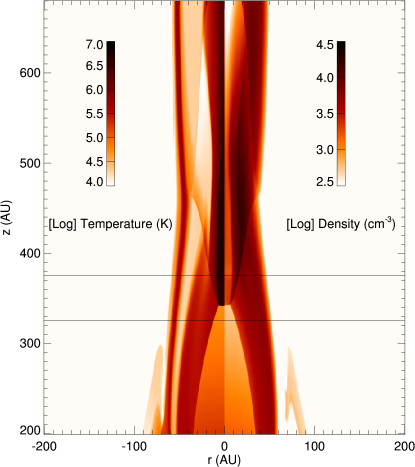
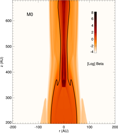
Figure 1: Two-dimensional maps of temperature (left half-panel on the left), density (right half-panel on the left), and plasma $\beta$ (on the right), after $t\approx 50$ years of evolution for the model M0. The contour $\beta=1$ is plotted in black on the right panel. The black horizontal lines plotted on the left panel correspond to $z=325$ and $z=375$, which are the radial profiles on the right panels in Figure 3.

Figure 2: Magnitude of the jet velocity (solid line), Alfven velocity (dotted line) and sound speed (dashed line) profiles at $r=0$ and $t\approx 50$ yr for the model M0. The shock is indicated.

Figure 3: Density (upper panels) and temperature (lower panels) profiles at $t\approx 50$ yr for the model M0 (see left panel in Fig. 1 for the 2D distributions). On the left, $z$ profiles at $r=0$; on the right, radial profiles at $z=325$ AU (dotted lines), and at $z=375$ AU (solid lines). We indicate the position of the normal and oblique shocks in the upper panels.

Figure 4: Density (solid line) and temperature (dotted line) profiles at $r=0$ and $t\approx 50$ yr for the model M0. Larger scales are used in order to show two consecutive shocks.

3.2 Exploration of the parameter space

We perform a broad exploration of the parameter space defined by the four free parameters: magnetic field strength along the $z$ axis, $B_{\mathrm{z}}$, maximum linear rotational velocity, $v_{\varphi,\mathrm{max}}$, jet velocity, $v_{\mathrm{j}}$, and jet density, $n_{\mathrm{j}}$ (see Sect. 2.2 and Table 1). The aim is to determine the range of parameters leading to the formation of a stationary shock emitting in X-rays.

We summarize in Table 2 the main physical parameters of the first shock diamond resulting from the different models defined in Table 1, namely, the shock position, maximum density and temperature, average temperature, mass and X-ray luminosity. We obtain shock temperatures ranging from $\sim 1\cdot 10^{6}$ to $\sim 5\cdot 10^{6}$ K, in excellent agreement with the X-ray observations of Favata et al. (2002) and Bally et al. (2003). The shock luminosity, $L_{\mathrm{X}}$, is calculated considering the whole region including the shock diamond.

In models M1-M5 we study the role of the magnetic field on the collimation of the jet and the location, stability and detectability in X-rays of the stationary shock. Model M5 considers a very low magnetic field strength (0.1 mG) and, in this case, no shock diamonds form in the computational domain; such a low magnetic field has not enough strength to collimate the jet. In models M3 and M4 the plasma is roughly collimated and a faint shock forms far from the base of the jet. Finally, in models M1 and M2 the shock also forms at large distances from the base of the jet but its X-ray luminosity is higher than that in models M3 and M4 because the shock is more extended in comparison with the reference case and the mass contributing to the X-ray emission is higher (see Table 2). In models M6-M8 we study the influence of introducing an angular velocity twisting the magnetic field lines and producing a helicoidal magnetic field. We describe in detail the latter three cases in Sect. 3.5 where we explore the role of the magnetic field twisting. In models M9-M13 we study the effect of changing the jet velocity, $v_{\mathrm{j}}$. In models M9-M11, with lower velocities respect to the reference case, we find that the shock forms closer to the magnetic nozzle than in the reference case and is more extended. Even the shock temperature and density are lower respect to the reference case, they show higher X-ray luminosities as the total mass contributing to the X-ray emission is higher. However, in models with higher velocities (M12-M13), the shock forms further and has lower luminosity. Lastly, we study the effect of increasing the jet density, $n_{\mathrm{j}}$, in model M14. In this case we obtain a very low luminosity comparing with the other cases, as the mass contributing to the X-ray emission is very low (see Table 2).

Considering the physical parameters from the different models shown in Table 2, the most promising cases are M0 (the reference case), M6-M8 (the models considering the magnetic field twisting), and M9-M11 (the models with lower jet velocities). In all these cases a stationary shock forms close to the base of the jet and, as discussed in Sect. 3.4, its X-ray luminosity is comparable with those observed (Favata et al., 2002; Bally et al., 2003; Güdel et al., 2008; Schneider et al., 2011; Skinner et al., 2011).

Table 2: Summary of the main physical parameters resulting from the different models: shock position (shock starting position from the beginning of the domain), $d_{\mathrm{s}}$, shock maximum density, $n_{\mathrm{s,max}}$, shock maximum temperature, $T_{\mathrm{s,max}}$, shock temperature (calculated as the density-weighted average temperature), $T_{\mathrm{s}}$, shock mass, $m_{\mathrm{s}}$, and shock X-ray luminosity, $L_{\mathrm{X}}$. For the calculation of the shock temperature and mass, $T_{\mathrm{s}}$ and $m_{\mathrm{s}}$ respectively, we only consider the cells with $T\geq 10^{6}$ in order to describe the shock X-ray emission contribution.

Model	$d_{\mathrm{s}}$ (AU)	$n_{\mathrm{s,max}}$ ($10^{4}$ cm-3)	$T_{\mathrm{s,max}}$ (MK)	$T_{\mathrm{s}}$ (MK)	$m_{\mathrm{s}}$ ($10^{-9}M_{\odot}$)	$L_{\mathrm{X}}$ ($10^{28}$ erg s-1)
M0	$340$	$1.7$	$5.8$	$2.1$	$1.7$	$8.8$
M1	$430$	$1.7$	$4.7$	$2.8$	$2.4$	$9.3$
M2	$570$	$1.9$	$5.7$	$2.5$	$2.2$	$9.3$
M3	$910$	$1.8$	$7.0$	$2.4$	$1.7$	$6.3$
M4	$1950$	$1.1$	$6.3$	$2.3$	$1.1$	$4.7$
M5	no shock diamond formed
M6	$340$	$1.7$	$5.8$	$1.9$	$2.0$	$11.5$
M7	$340$	$1.5$	$4.7$	$1.9$	$2.5$	$15.7$
M8	$320$	$1.3$	$4.7$	$2.2$	$3.1$	$22.1$
M9	$160$	$0.7$	$1.4$	$1.2$	$2.7$	$15.0$
M10	$230$	$1.1$	$2.3$	$1.8$	$2.9$	$17.8$
M11	$290$	$1.4$	$3.5$	$2.3$	$2.1$	$11.7$
M12	$530$	$2.6$	$2.7$	$1.5$	$2.0$	$5.4$
M13	$550$	$2.3$	$5.2$	$1.4$	$1.7$	$6.2$
M14	$450$	$302$	$3.6$	$1.3$	$0.06$	$0.05$

3.3 Emission measure distribution vs. temperature

We derive the distribution of emission measure vs. temperature, $EM(T)$, in the temperature range $[10^{4}-10^{8}]$ K. The $EM(T)$ distribution is an important source of information of the plasma components with different temperature contributing to the emission and is very useful to compare model results with observations. We calculate the $EM(T)$ distribution as follows. First we derive the 2D distributions of temperature and density, by integrating the MHD equations in the whole spatial domain. Then we reconstruct the 3D spatial distribution of these physical quantities by rotating the 2D slabs around the symmetry axis $z$. For each cell of the 3D domain, we derive the emission measure defined as $EM=\int n_{\mathrm{e}}n_{\mathrm{H}}\mathrm{d}V$ (where $n_{\mathrm{e}}$ and $n_{\mathrm{H}}$ are the electron and hydrogen densities, respectively, and $V$ is the volume of emitting plasma). From the 3D spatial distributions of $T$ and $EM$, we derive the $EM(T)$ distribution for the computational domain as a whole or for part of it: we consider the temperature range $[10^{4}-10^{8}]$ K divided into 80 bins equispaced in log $T$; the total $EM$ in each temperature bin is obtained by summing the emission measure of all the fluid elements corresponding to the same temperature bin.

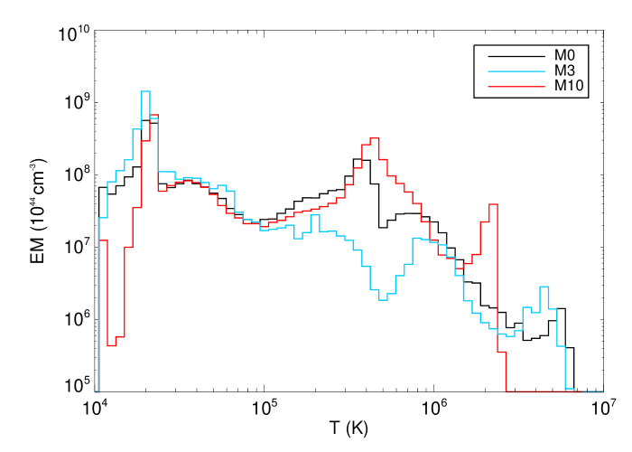
Figure 5: Emission measure, $EM$, distribution as a function of the temperature, $T$, after $\approx 50$ years of evolution. We compare different models: M0 (the reference case) in black, M3 (one of the less luminous cases) in blue, and M10 (the most luminous case without twisting) in red.

Figure 5 shows the $EM(T)$ for the reference case, M0 (see Sect. 3.1), after $\approx 50$ years of evolution for the region shown in Fig. 1, corresponding to the first shock. We find that the shape of the $EM(T)$ is characterized by three bumps at $T\approx 2\cdot 10^{4}$ K, $\approx 5\cdot 10^{5}$ K, and $\approx 6\cdot 10^{6}$ K. The latter corresponds to the shock diamond. The $EM$ decreases rapidly above few millions degrees. The same figure compares the $EM(T)$ distribution derived for M0 with those derived for models M3 (blue histogram) and M10 (red histogram). In the former, after a peak of $EM$ at $T\approx 2\cdot 10^{4}$ K, the $EM$ decreases gradually with the temperature, showing two bumps at $T\approx 10^{6}$ K and $T\approx 5\cdot 10^{6}$ K. The $EM$ is lower than that in model M0 and, as a consequence, the X-ray luminosity is expected to be much lower too. Conversely, model M10 shows two intense bumps centred at $T\approx 7\cdot 10^{5}$ K and $T\approx 3\cdot 10^{6}$ K with high values of $EM$. We expect therefore that this model produces higher values of X-ray luminosity.

3.4 Spatial distribution of X-ray emission

From the 3D spatial distributions of temperature and density reconstructed from the 2.5D simulations (see Sect. 3.3), we synthesize the emission in the [0.3-10] keV band to compare the model results with the observations. In particular we derive 2D X-ray images by integrating the X-ray emission along the line of sight (assumed to be perpendicular to the jet axis).

Figure 6 shows the spatial distribution of the X-ray emission for the reference case, M0 (see Sect. 3.1), for M3 (one of the less luminous cases) and M10 (the most luminous case without twisting), after 48 years of evolution. The X-ray source appears as a single elongated source corresponding to the shock diamond region developing as a result of the jet collimation (see discussion in Sect. 3.1). Note the different scale for the $z$ axis in the three panels of the figure and also with respect to Fig. 1. After an initial transient ($\sim 10$ yr), all these sources appear to be stationary over the time covered by the simulations ($\sim 50$ yr; see the movie provided online). Almost all the X-ray emission originates from the shock diamond, whereas the contribution arising from the jet envelope is negligible in all the cases.

The X-ray total shock luminosity, $L_{\mathrm{X}}$, in the [0.3-10] keV band, derived for the model M0 is $\sim 9\cdot 10^{28}$ erg s^-1 (see Table 2). The spatial X-rays distribution for the model M10 has wider shape and higher total shock luminosity, namely $\sim 2\cdot 10^{29}$ erg s^-1. Finally, the spatial X-rays distribution for the model M3 is fainter and more extended, with a total shock luminosity of $\sim 6\cdot 10^{28}$ erg s^-1. These values are comparable with those detected in several HH objects (Favata et al., 2002; Bally et al., 2003; Güdel et al., 2008; Schneider et al., 2011; Skinner et al., 2011), ranging between $2.4\cdot 10^{28}$ and $3\cdot 10^{29}$ erg s^-1.

Note that the X-ray luminosity, $L_{\mathrm{X}}$, is calculated assuming that the plasma is optically thin. In order to verify our assumption, we estimated a hydrogen column density $N_{\mathrm{H}}\approx 9\cdot 10^{17}$ cm^-2, assuming a shock thickness of 60 AU and a density of $10^{3}$ cm^-3. Thus, the X-ray absorption is negligible.

It is also worth noting that hydrodynamic models predict significant X-ray emission by jets less dense than the ambient medium (light jets), whereas jets denser than the ambient (heavy jets) produce X-ray luminosities even several orders of magnitude lower than those observed (e.g. Bonito et al. 2011). Our results show that the magnetic field can enhance the X-ray luminosity from jets, leading to X-ray luminosities comparable with those observed even in the case of heavy jets. Here we suggest that the magnetic field plays a fundamental role in observed X-ray emitting heavy jets through efficient magnetic collimation of the flow in shock diamonds.

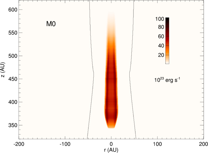
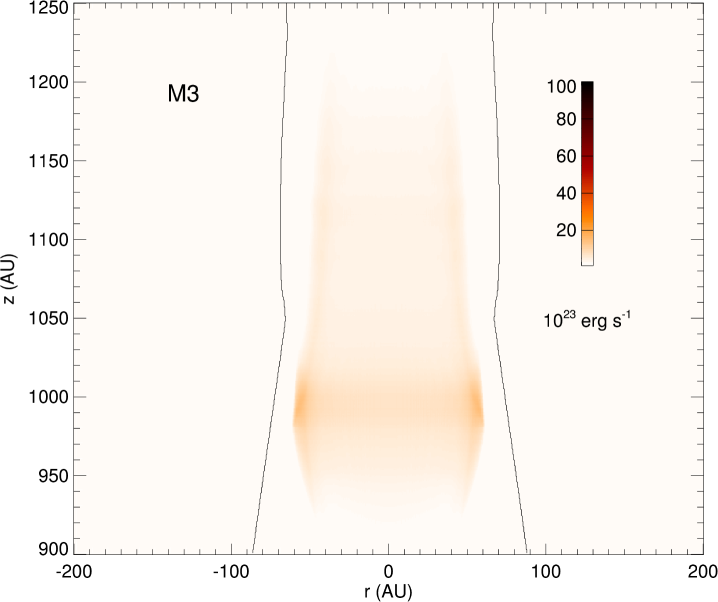
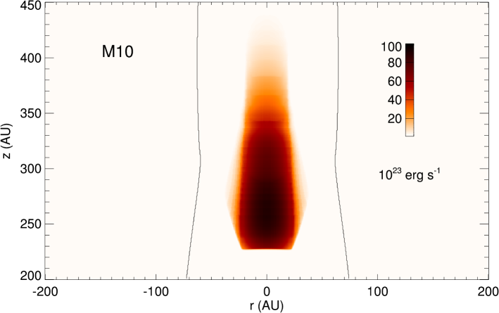
Figure 6: Spatial distribution of the X-ray emission after $\approx 50$ years of evolution. We compare different models: M0 (the reference case) upper panel, M3 (one of the less luminous cases) middle panel, and M10 (the most luminous case without twisting) in the lower panel. We plot the contour of the jet in black in each case.

3.5 Role of the jet rotational velocity

In models M6, M7 and M8 (see Table 1) we study the influence of introducing an angular velocity to the jet. We define a constant angular velocity producing maximum linear rotational velocity values, $v_{\varphi,\mathrm{max}}$, ranging from 75 to 150 km s^-1 at the lower boundary. The jet rotation produces a toroidal component at the initially axial magnetic field achieving a helicoidal configuration during the simulation. The final configuration of the magnetic field depends on the rotational velocity of the plasma; the higher the velocity, the more twisted the magnetic field lines. In Figure 7 we show a 3D representation of the density distribution and magnetic field configuration for model M8, the one with the highest rotational velocity of the cases explored (see Table 1). The magnetic field lines are twisted in a helicoidal configuration, contributing to the jet collimation.

In Figure 8 we show two-dimensional maps of the plasma $\beta$ for the three models. We can distinguish two different regimes in all the cases: the area close to the jet axis where $\beta>1$, dominated by the jet plasma pressure, in contrast to the rest of the domain where $\beta<1$, dominated by the magnetic field. According to the maps, the higher the rotational velocity the larger the region with $\beta>1$, dominated by the jet plasma pressure, and the stronger and more extended the shock. This is basically due to the increase of the dynamic pressure in the jet interior.

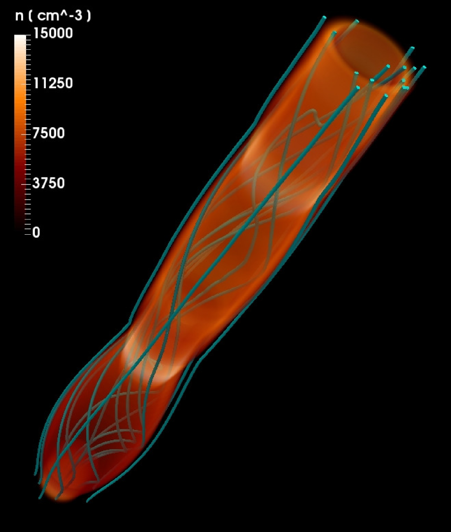
Figure 7: 3D representation of the density distribution and the magnetic field configuration (blue lines) for the model M8 after $\approx 50$ years of evolution.

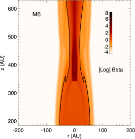
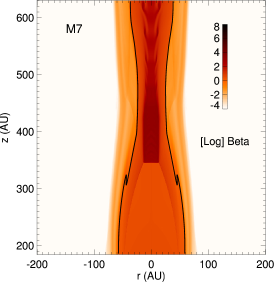
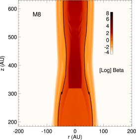
Figure 8: Two-dimensional maps of plasma $\beta$ after $\approx 50$ years of evolution. Different models are compared: M6 (the model with the lowest rotational velocity) left panel, M7 (the model with an intermediate rotational velocity) middle panel, and M8 (the model with the highest rotational velocity) right panel. The contour $\beta=1$ is plotted in black in every case.

Figure 9 shows the emission measure distribution vs. temperature, $EM(T)$, calculated as explained in Section 3.3. We compare the reference case, M0, with the models M6, M7 and M8 (see Table 1); this allows us to explore the effect of an increasing angular velocity and the expected emission from the jet. We find that, increasing the rotational velocity $v_{\varphi,\mathrm{max}}$, the $EM$ decreases for temperatures $T<6\cdot 10^{5}$ K and increases for higher temperatures. Thus we expect that, increasing $v_{\varphi,\mathrm{max}}$, the shock diamond is a brighter X-ray source with higher X-ray luminosity.

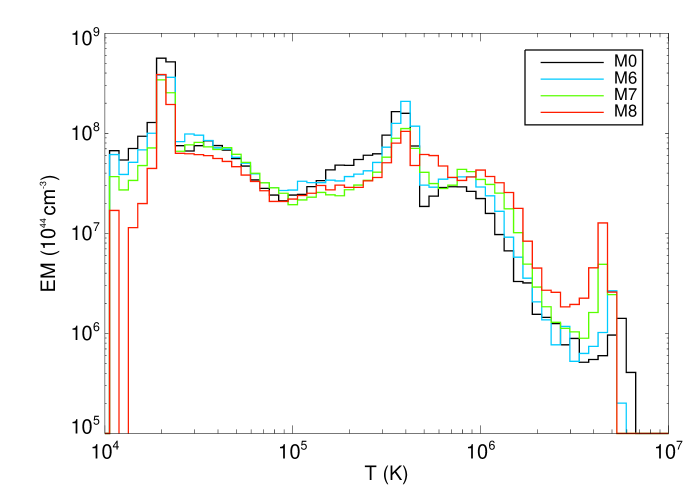
Figure 9: Emission measure, $EM$, distribution as a function of the temperature, $T$, after $\approx 50$ years of evolution. We compare different models: M0 (the reference case) in black, M6 (the model with the lowest rotational velocity) in blue, M7 (the model with an intermediate rotational velocity) in green, and M8 (the model with the highest rotational velocity) in red.

Figure 10 shows the spatial distribution of the X-ray emission for the three different models with twisting (see Table 1), derived as explained in Section 3.4. We find that the X-ray emission source, corresponding to the shock diamond, is closer to the base of the jet and more extended for models with higher jet rotation velocities. The X-ray total shock luminosity, $L_{\mathrm{X}}$, in the [0.3-10] keV band, is larger for higher rotational velocity of the jet (see Table 2), as the total mass contributing to the X-ray emission is higher. These values are consistent with those detected in several HH objects (Favata et al., 2002; Bally et al., 2003; Güdel et al., 2008; Schneider et al., 2011; Skinner et al., 2011).

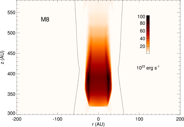
Figure 10: Spatial distribution of the X-ray emission after $\approx 50$ years of evolution. Different models are compared: M6 (the model with the lowest rotational velocity) upper panel, M7 (the model with an intermediate rotational velocity) middle panel, and M8 (the model with the highest rotational velocity) lower panel. We plot the contour of the jet in black in each case.

From the models, we also calculate the density-weighted average velocity along the line of sight and compare it with the velocities inferred from the observations (Bacciotti et al., 2002; Coffey et al., 2004, 2007; Woitas et al., 2005). We consider the line of sight perpendicular to the jet axis and we degrade the spatial resolution of the maps derived from the simulations from 0.5 AU to 20 AU (typical average resolution achieved in observations). In Figure 11, we show two-dimensional distributions for the density-weighted velocities along the line of sight for M6, M7 and M8 obtained with spatial resolution of 20 AU. We find similar characteristics in the three cases. The projected velocities are larger at the edge of the jet where strong $B_{\varphi}$ and $B_{\mathrm{r}}$ components are generated collimating the jet. The velocity reaches its maximum $v_{\mathrm{max}}$ in proximity of the first shock diamond where $v_{\mathrm{max}}\approx 60$ km s^-1 for model M6, and $v_{\mathrm{max}}\approx 70$ km s^-1 for models M7 and M8. The values derived in the pre-shock region are quite lower: maximum values for M6, M7 and M8 are $\sim 30$ km s^-1, $\sim 40$ km s^-1 and $\sim 50$ km s^-1 respectively. The velocities are significantly lower close to the jet axis where $v_{\mathrm{max}}<10$ km s^-1. All these values are compatible with those inferred from the observations by Bacciotti et al. (2002).

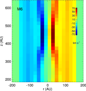
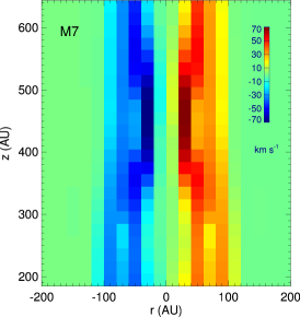
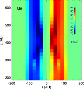
Figure 11: Density-weighted rotational velocity along the line of sight with macropixel resolution of 20 AU after $\approx 50$ years of evolution. Different models are compared: M6 (the model with the lowest rotational velocity) left panel, M7 (the model with an intermediate rotational velocity) middle panel, and M8 (the model with the highest rotational velocity) right panel.

3.6 Role of thermal conduction and radiative losses

We perform some additional simulations for the reference case (see Sect. 3.1) in order to investigate more deeply the role of thermal conduction and radiative losses in the model. We perform three extra simulations: M0-id, the model M0 for the ideal case (without thermal conduction and cooling); M0-rd, the model M0 including only the radiative cooling; and M0-th, the model M0 including only the thermal conduction. We show the main physical parameters resulting from the different simulations performed in Table 3. The jet morphology and the shock position are similar in all the cases, although other shock properties show relevant differences.

Table 3: Summary of the main physical parameters resulting from the different simulations performed for the reference case, M0 (see Table 1): shock position (shock starting position from the beginning of the domain), $d_{\mathrm{s}}$, shock maximum density, $n_{\mathrm{s,max}}$, shock maximum temperature, $T_{\mathrm{s,max}}$, shock temperature (calculated as the density-weighted average temperature), $T_{\mathrm{s}}$, shock mass, $m_{\mathrm{s}}$, and shock X-ray luminosity, $L_{\mathrm{X}}$. For the calculation of the shock temperature and mass, $T_{\mathrm{s}}$ and $m_{\mathrm{s}}$ respectively, we only consider the cells with $T\geq 10^{6}$ in order to describe the shock X-ray emission contribution. M0-id is the model M0 for the ideal case (without thermal conduction and cooling), M0-rd is the model M0 including only the radiative cooling, and M0-th is the model M0 including only the thermal conduction.

Model	$d_{\mathrm{s}}$ (AU)	$n_{\mathrm{s,max}}$ ($10^{4}$ cm-3)	$T_{\mathrm{s,max}}$ (MK)	$T_{\mathrm{s}}$ (MK)	$m_{\mathrm{s}}$ ($10^{-9}M_{\odot}$)	$L_{\mathrm{X}}$ ($10^{28}$ erg s-1)
M0	$340$	$1.7$	$5.8$	$2.1$	$1.7$	$8.8$
M0-id	$340$	$0.8$	$4.9$	$1.5$	$3.4$	$35.3$
M0-rd	$340$	$1.7$	$5.0$	$2.1$	$1.8$	$9.1$
M0-th	$340$	$0.8$	$6.8$	$1.5$	$3.3$	$34.8$

In Figure 12 we compare the emission measure distribution vs. temperature, $EM(T)$, for the different models. The upper panel in the figure highlights the effect of radiative losses on the structure of the shock diamond by comparing models M0-id and M0-rd: the effects of cooling determines a decrease of $EM$ at $T>10^{6}$ K and an increase of $EM$ at lower temperatures. This is due to the gradual cooling of the plasma in the shock diamond. The middle panel in Fig. 12 shows the effect of the thermal conduction by comparing models M0-id and M0-th. In this case we note that the thermal conduction has a rather marginal effect in shaping the $EM(T)$ distribution, slightly increasing the $EM$ of plasma with $T>10^{5}$ K and decreasing the $EM$ at $T<10^{5}$ K. In Figure 13 we compare the profiles for density, temperature and velocity for models M0-id and M0-th. The thermal conduction leads to higher values of temperature in the post-shock region, although the pre-shock temperature is the same in both cases (see center panel in Fig. 13). This difference is also reflected in the velocity profiles which show lower values for model M0-th at the shock, even with negative values (see right panel in Fig. 13), forming a vortex shape velocity field. By comparing models including the radiative losses, namely runs M0 and M0-rd (see upper and lower panels in Fig. 12), we find that the corresponding $EM(T)$ distributions show similar shapes, thus demonstrating that the structure of the jet is largely dominated by the radiative cooling. The main differences between the two appear for high temperatures ($>10^{6}$ K), corresponding to the shock diamond area where the thermal conduction is more efficient and has some effect.

For the different models, we obtain slightly different values for the temperature and density in the shock diamond (see Table 3), and we find that the corresponding synthetic luminosities are lower ($\sim 10^{29}$ erg s^-1) for models with radiative cooling (M0 and M0-rd). The models not considering radiative cooling (M0-id and M0-th) show more extended X-ray sources (see Figure 14) and higher luminosities ($\sim 3\cdot 10^{29}$ erg s^-1).

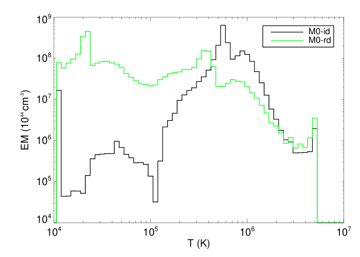
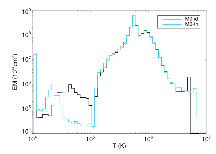
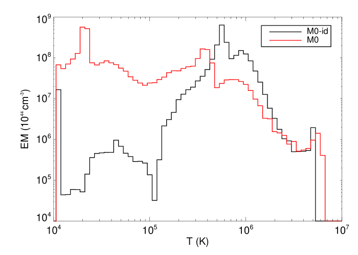
Figure 12: Emission measure, $EM$, distribution as a function of the temperature, $T$, after $\approx 50$ years of evolution. Different models are compared: M0-rd in green (upper panel), M0-th in blue (middle panel), and M0 in red (lower panel). The $EM(T)$ for the model M0-id is represented by black line in all panels.

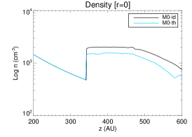
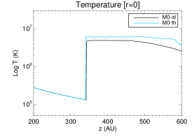
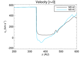
Figure 13: Density (left panel), temperature (middle panel) and velocity (right panel) profiles at $r=0$ and $t\approx 50$ yr. We compare the ideal MHD model (M0-id) in black with the model including the thermal conduction (M0-th) in blue.

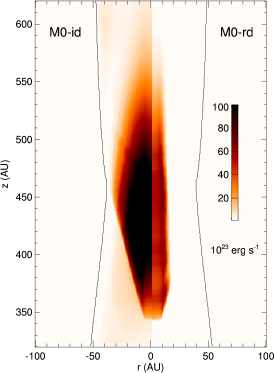
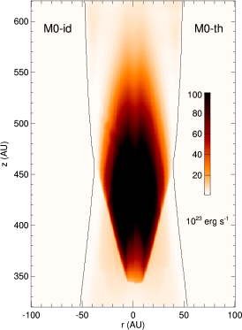
Figure 14: Spatial distribution of the X-ray emission after $\approx 50$ years of evolution. Different models are compared: M0-rd (the model with radiative cooling) right half-panel on the left, M0-th (the model with thermal conduction) right half-panel in the middle, and M0 (the reference case) right half-panel on the right. The X-ray distribution for the model M0-id is reported in each left half-panel.

4 Discussion and conclusions

The analysis of the observations of HH154 in three different epochs with Chandra (Bally et al., 2003; Favata et al., 2006; Schneider et al., 2011; Bonito et al., 2011) revealed a faint and elongated X-ray source at some 150 AU from the protostar that appeared to be quasi-stationary over a time base of $\sim 8$ yr without appreciable proper motion and variability of X-ray luminosity and temperature. Also, the best-studied bright, central X-ray jet of DG Tau seemed to be stationary on timescales of several years on spatial scales of about 30 AU from the central star (Schneider & Schmitt, 2008). One of the viable models proposed by Bonito et al. (2011) on the base of hydrodynamic modelling, explained the observations of HH154 describing a shock diamond formed at the opening of a nozzle and producing a X-ray stationary source. They propose a magnetic nozzle as the origin of the shock and they derive a magnetic field strength $B\approx 5$ mG in the magnetic nozzle at the base of the jet.

Following the above line of research, we proposed here a new MHD model which describes the propagation of a jet through a magnetic nozzle which rams with a supersonic speed into an initially isothermal and homogeneous magnetized medium. Our MHD model takes into account, for the first time, the relevant physical effects, including the radiative losses from optically thin plasma and the magnetic field oriented thermal conduction.

We investigated how the magnetic nozzle contributes to the jet collimation and, possibly, to the formation of a shock diamond at the exit of the nozzle. To this end, we performed an extensive exploration of the parameter space that describes the model. These results allowed us to study and diagnose the properties of protostellar jets over a broad range of physical conditions and to determine the physical properties of the shocked plasma. The different parameters considered are shown in Table 1.

We found that a minimum magnetic field ($\sim 1-2$ mG) is necessary to collimate the plasma and form a train of shock diamonds. We selected a magnetic field strength of 5 mG as reference case. For lower values of magnetic field strength, we found that the shock forms at larger distances from the driving star and the beam radius is wider than those usually observed. We found that the stronger is the magnetic field and the lower is the flow velocity, the closer forms the shock to the base of the jet. The summary of results shown in Table 2 could be very useful in some cases to constrain part of the main physical parameters of protostellar jets from those already known.

We derived the physical parameters of a protostellar jet that can give rise to stationary X-ray sources at the base of the jet consistent with observations of HH objects. We found that, in most of the cases explored, quasi-stationary X-ray emission originates from the first shock diamond close to the base of the jet. We obtained shock temperatures of $\sim 1-5\cdot 10^{6}$ K, in excellent agreement with the X-ray results of Favata et al. (2002) and Bally et al. (2003). X-ray emission from several HH objects was detected with both the XMM-Newton and Chandra satellites: HH2 in Orion (Pravdo et al., 2001), HH154 in Taurus (Favata et al., 2002; Bally et al., 2003), HH168 in Cepheus A (Pravdo & Tsuboi, 2005), and HH80 in Sagittarius (López-Santiago et al., 2013). They showed luminosities of $L_{\mathrm{X}}\approx 10^{29}-10^{30}$ erg s^-1. Other cases well studied, as Taurus jets of L1551 IRS-5, DG Tau, and RY Tau, showed luminous ($L_{\mathrm{X}}\approx 10^{28}-10^{29}$ erg s^-1) X-ray sources at distances corresponding to 30-140 AU from the driving star (Favata et al., 2002; Bally et al., 2003; Güdel et al., 2008; Schneider et al., 2011; Skinner et al., 2011). The parameters used in our model and the luminosity values synthesized from the model results are in good agreement with those observed: our reference case predicts a luminosity $L_{\mathrm{X}}\approx 10^{29}$ erg s^-1 which is in good agreement with observed values. The cases with higher observed luminosities, as HH154, are in good agreement with models M9-M11 (with lower velocities), and M6-M8 (with magnetic field twisting). We obtain the highest luminosity in the model M8, the model with the highest jet rotational velocity.

In additon, we investigated the effect of jet rotation on the structure of shock diamonds. Several detections of gradients in the radial velocity profile across jets from T Tauri stars were reported (Bacciotti et al., 2002; Coffey et al., 2004, 2007; Woitas et al., 2005). These velocity shifts might be interpreted as signatures of jet rotation about its symmetry axis. For example, Bacciotti et al. (2002) derived toroidal velocities of the emitting regions between 6 and 15 km s^-1, depending on position. Woitas et al. (2005) gave higher toroidal velocities in the range 5-30 km s^-1. They interpreted these velocity asymmetries as rotation signatures in the region where the jet has been collimated but has not yet manifestly interacted with the environment. Considering our model, this region corresponds to the bottom part of the velocity maps in Fig. 11 with values $5-30$ km s^-1 for model M6, $6-40$ km s^-1 for model M7 and $7-50$ km s^-1 for model M8. Alternative interpretations include asymmetric shocking and/or jet precession (e.g., Soker, 2005; Cerqueira et al., 2006; Correia et al., 2009).

We derived the angular momentum loss rate at the base of the jet for the three models, M6, M7 and M8 as $\dot{J}_{\mathrm{j},\omega}=\int\rho_{\mathrm{j}}v_{\mathrm{j}}v_{\varphi}r\,\mathrm{d}A$, where $\rho_{\mathrm{j}}$ and $v_{\mathrm{j}}$ are the mass density and jet velocity, respectively, $v_{\varphi}$ is the rotational velocity, $r$ is the radius and $\mathrm{d}A$ is the cross sectional area of the incoming jet plasma. The values obtained range between $1.63\cdot 10^{-5}$ $M_{\odot}$ yr^-1 AU km s^-1 for model M6 and $3.25\cdot 10^{-5}$ $M_{\odot}$ yr^-1 AU km s^-1 for model M8. These values refer to the flux carried away by the jet and they are in good agreement with that estimated by Bacciotti et al. (2002), namely, $3.8\cdot 10^{-5}$ $M_{\odot}$ yr^-1 AU km s^-1. Thus, our model could be a useful tool for the investigation of the still debated rotation of the jets.

We also explored the role of thermal conduction and radiative losses in determining the structure of the shock diamonds by performing some extra simulations calculated with these physical processes turned “on” or “off”. We found that the radiative losses dominate the evolution of the shocked plasma in the diamonds. The main effect is to decrease the $EM$ of plasma with temperature larger than $10^{6}$ K, thus reducing its X-ray luminosity. The thermal conduction plays a minor role slightly contrasting the cooling of hot plasma due to radiative losses.

The comparison between our model results and the observational findings showed that the model reproduces most of the physical properties observed in the X-ray emission of protostellar jets (temperature, emission measure, X-ray luminosity, etc.). Thus we showed the feasibility of the physical principle on which our model is based: a supersonic protostellar jet leads to X-ray emission from a stationary shock diamond, formed after the jet is collimated by the magnetic field, consistent with the observations of several HH objects. We conclude that our model provides a simple and natural explanation for the origin of stationary X-ray sources at the base of protostellar jets. Therefore, the comparison of our MHD model results with the X-ray observations could provide a fundamental tool to investigate the role of the magnetic field on the protostellar jet dynamics and X-ray emission.