The Stability of Tidal Equilibrium
for Hierarchical Star-Planet-Moon Systems

Abstract

Motivated by the current search for exomoons, this paper considers the stability of tidal equilibrium for hierarchical three-body systems containing a star, a planet, and a moon. In this treatment, the energy and angular momentum budgets include contributions from the planetary orbit, lunar orbit, stellar spin, planetary spin, and lunar spin. The goal is to determine the optimized energy state of the system subject to the constraint of constant angular momentum. Due to the lack of a closed form solution for the full three-body problem, however, we must use use an approximate description of the orbits. We first consider the Keplerian limit and find that the critical energy states are saddle points, rather than minima, so that these hierarchical systems have no stable tidal equilibrium states. We then generalize the calculation so that the lunar orbit is described by a time-averaged version of the circular restricted three-body problem. In this latter case, the critical energy state is a shallow minimum, so that a tidal equilibrium state exists. In both cases, however, the lunar orbit for the critical point lies outside the boundary (roughly half the Hill radius) where (previous) numerical simulations indicate dynamical instability. These results suggest that star-planet-moon systems have no viable long-term stable states analogous to those found for two-body systems.

1 Introduction

A classic dynamical problem is to consider the tidal equilibrium states for self-gravitating systems that include both rotational and orbital motion (Darwin, 1879, 1880). The conditions required for the existence of such equilibrium states has been determined previously for binary star systems (Counselman, 1973; Hut, 1980). With the relatively recent discovery of exoplanets, this problem has received renewed interest (Levrard et al., 2009; Matsumura et al., 2010; Adams & Bloch, 2015). In this contribution, we extend previous treatments to include the presence of a satellite or moon orbiting the secondary (see also Barnes & O’Brien 2002; Jacobson & Scheeres 2011). We thus consider the existence of tidal equilibrium states for hierarchical triple systems consisting of a star, planet, and moon, where all three bodies have spin angular momentum.

Although the discovery of moons in extrasolar planetary systems has not yet been realized, they have generated great interest. Now that the existence of exoplanets is well established, and their populations are being characterized, the next astronomical frontier is to discover moons in other solar systems. These additional bodies are in principle observable through their transit timing variations (Kipping, 2009), wherein additional bodies in a planetary system change the times at which the planet casts shadows on the host star (Agol et al., 2005; Holman & Murray, 2005). These moons are most readily detected if they have large relative masses and their host planets orbit near the star. Another regime of interest is that of potentially habitable moons, where the orbit of the host planet resides within the habitable zone (Kasting et al., 1993) of its star. In this case, a moon orbiting the planet could be potentially habitable provided that it has the proper mass, atmosphere, and other characteristics (Kipping et al., 2009; Heller et al., 2014). In both regimes, however, moons are susceptible to removal (Donnison, 2010; Weidner & Horne, 2010; Spalding et al., 2016).

In general, systems evolve toward lower energy states, but are required to conserve their total angular momentum (in the absence of external torques). For two-body systems, previous treatments show that three evolutionary paths are available: [A] The orbit of the secondary can decay inward and eventually collide with the primary, where the orbital angular momentum is transferred to the rotation of the primary. [B] The orbit can gain angular momentum from the primary and move outwards toward an unbound state. [C] The system can approach a stable tidal equilibrium configuration, where the orbit and spins of both bodies have the same period and their angular momentum vectors point in the same direction. The Pluto-Charon system provides one such example (Tholen et al., 1987). In order for the equilibrium state to exist, the system must have a minimum amount of total angular momentum; in order for the system to reside in the equilibrium state, its orbital angular momentum must be at least three times larger than the spin angular momentum. The goal of this paper is to derive analogous requirements for the existence of stable tidal equilibrium states for hierarchical three-body systems (star-planet-moon systems).

The existence of tidal equilibrium states does not depend directly on the energy dissipation mechanisms that allow systems to attain such states. In the cases of interest, the relevant dissipative evolution is generally driven by tidal effects (Hut, 1981; Zahn, 1977). Since tidal evolution occurs over long time scales, often comparable to the age of the universe, many extant systems are not expected to have reached their lowest energy states. Notice also that tidal equilibrium is determined under the assumption of conservation of angular momentum, which must exceed a minimum value for the equilibrium state to exist. Although planetary systems can lose angular momentum via stellar winds and other astronomical processes, systems that start with too little angular momentum generally have no means of gaining more.

In the regimes of interest, the host planet often has mass comparable to Jupiter and the moon has mass comparable to Earth. This satellite mass is favored because it is large enough to produce measurable transit timing variations in Hot Jupiter systems and large enough to be potentially habitable in systems with more temperate Jupiters. Here we denote the masses of the three bodies as $M$ for the star, $m$ for the planet, and $\mu$ for the moon. These masses are assumed to obey the ordering

$$\mu\ll{m}\ll{M}.$$ (1)

This work assumes that the planetary orbit (about the star) has semimajor axis $a$ and the moon orbit (about the planet) has semimajor axis $b$ (when the moon orbits within a non-Keplerian potential, the scale $b$ refers to the radius of the lunar orbit). The star has spin angular momentum with moment of inertia $I$ and rotation rate $\Omega$. The planet also has spin angular momentum with moment of inertia $J$ and rotation rate $\omega$. Finally, the moon has moment of inertia $K$ and rotation rate $\lambda$. Because of the mass ordering from equation (1), we can ignore the difference between the reduced mass and the actual mass of an orbiting body.

A great deal of previous work has considered the dynamics of these hierarchical systems (Szebehely, 1967, 1978). However, most of the work regarding system stability does not include the effects of rotation of the bodies (see the review of Georgakarakos 2008). As shown previously for two-body systems, the possible exchange of angular momentum between the orbit(s) and rotation plays an important role in determining tidal equilibrium states. We also note that many previous numerical simulations (e.g., Payne et al. 2013 and references therein) have shown that the long-term dynamical stability of the system requires the lunar orbit to fall within some fraction $f$ of the Hill radius $(b<fR_{H})$, where $R_{H}\equiv(m/3M)^{1/3}a$ and $f\sim 1/2$. These numerical studies generally do not include rotational angular momentum, but provide independent constraints on the stability of star-planet-moon systems. Significantly, the results of this paper indicate that tidal equilibrium states — when they exist — correspond to lunar orbits that lie outside the stability regime found numerically. Finally, the tidal evolution of our moon, and others, including tidal dissipation has been studied in detail (Goldreich & Peale, 1966; Touma & Wisdom, 1994)). The dissipation time scales often exceed the age of the system, or even the age of the universe, so that observed systems are often not found in their lowest accessible energy states.

The goal of this paper is to consider the equilibrium states of the system, including the effects of stellar, planetary, and lunar rotation in the energy and angular momentum budgets. We first consider the problem in the limit where both the orbits can be described using Keplerian solutions (Section 2). For this case, we allow the five angular momentum vectors to have different directions and allow the orbits to have eccentricity. Nevertheless, the tidal equilibrium state corresponds to circular orbits and aligned angular momentum vectors. Moreover, the critical point is a saddle point, rather than a minimum, so that no stable tidal equilibrium state exists for this limiting case. We then generalize the problem to include the stellar influence on the lunar orbit, which is treated by a time-average of the circular restricted three-body problem (Section 3). For this case, the system has two critical points. The first corresponds to a saddle point, whereas the second corresponds to a minimum of the energy so that a stable tidal equilibrium state exists. In Section 4, we briefly consider applications of these results for extrasolar planetary systems, as well as moons in our Solar System. The paper concludes, in Section 5, with a summary of our results and a discussion of their implications.

2 Three-Body Systems in the Keplerian Limit

As a first approximation, we consider the orbits of both the planet and the moon to be described by standard Keplerian solutions. The energy and angular momentum of the system thus have five contributions: the planetary orbit around the star, the lunar orbit around the planet, stellar spin, planetary spin, and lunar spin. Because of the ordering of masses from equation (1), the center of mass of the system lies at the center of the star.

In physical units, the energy and anuglar momentum of the system are given by

$${E}=-{GMm\over 2a}-{Gm\mu\over 2b}+{1\over 2}I|{\vec{\Omega}}|^{2}+{1\over 2}J|{\vec{\omega}}|^{2}+{1\over 2}K|{\vec{\lambda}}|^{2}.$$ (2)

The first two terms arise from the energy of the two orbits and the next three terms arise from the rotational energy. The total angular momentum $\vec{L}$ is given by

$$\vec{L}={\vec{h}}+{\vec{k}}+I{\vec{\Omega}}+J{\vec{\omega}}+K{\vec{\lambda}}.$$ (3)

The orbital angular momenta of the planet $\vec{h}$ and moon $\vec{k}$ have magnitudes defined by

$${h}\equiv{m}\sqrt{GMa(1-e^{2})}\qquad{\rm and}\qquad{k}\equiv\mu\sqrt{Gmb(1-\epsilon^{2})},$$ (4)

where $e$ and $\epsilon$ are the eccentricities for the planetary and lunar orbit, respectively. In general, the five angular momentum vectors can have different directions. We choose the coordinate axes so that the total angular momentum vector of the system points in the ${\hat{z}}$ direction. The orbital angular momentum vector for the planetary orbit has direction given by ${\hat{h}}\cdot{\hat{z}}=\cos{i}$. Without loss of generality, we let the vector lie in the $x$-$z$ plane. Similarly, the angular momentum vector of the lunar orbit has direction given by ${\hat{k}}\cdot{\hat{z}}=\cos\theta$, where we introduce the azimuthal angle $\phi$ such that ${\hat{k}}\cdot{\hat{x}}=\sin\theta\cos\phi$ and ${\hat{k}}\cdot{\hat{y}}=\sin\theta\sin\phi$. With these definitions, the total angular momentum has $z$-component

$${L}=|{\vec{L}}|=L_{z}=h\cos{i}+k\cos\theta+I\Omega_{z}+J\omega_{z}+K\lambda_{z}.$$ (5)

The remaining components of the angular momentum vector must vanish so that

$${L_{x}}=h\sin{i}+k\sin\theta\cos\phi+I\Omega_{x}+J\omega_{x}+K\lambda_{x}=0,$$ (6)

and

$${L_{y}}=k\sin\theta\sin\phi+I\Omega_{y}+J\omega_{y}+K\lambda_{y}=0.$$ (7)

2.1 Equilibrium States of the System: First Variation

To simplify the calculation, we work in dimensionless units where $G=M=I=1$, so that the energy of the system takes the form

$${E}=-{m\over 2a}-{\mu m\over 2b}+{1\over 2}\left(\Omega_{x}^{2}+\Omega_{y}^{2}+\Omega_{z}^{2}\right)+{1\over 2}J\left(\omega_{x}^{2}+\omega_{y}^{2}+\omega_{z}^{2}\right)+{1\over 2}K\left(\lambda_{x}^{2}+\lambda_{y}^{2}+\lambda_{z}^{2}\right),$$ (8)

where the angular velocity vectors are written in terms of their components. Using conservation of angular momentum, we eliminate the stellar spin variables $(\Omega_{x},\Omega_{y},\Omega_{z})$ from the energy expression so it becomes

$${E}=-{m\over 2a}-{\mu m\over 2b}+{1\over 2}(L-h\cos{i}-k\cos\theta-J\omega_{z}-K\lambda_{z})^{2}+{1\over 2}(h\sin{i}+k\sin\theta\cos\phi+J\omega_{x}+K\lambda_{x})^{2}$$ (9)

$$+{1\over 2}(k\sin\theta\sin\phi+J\omega_{y}+K\lambda_{y})^{2}+{J\over 2}(\omega_{x}^{2}+\omega_{y}^{2}+\omega_{z}^{2})+{K\over 2}(\lambda_{x}^{2}+\lambda_{y}^{2}+\lambda_{z}^{2}).$$

In this form, the energy is a function of 13 variables $(a,b,e,\epsilon,i,\theta,\phi,\omega_{x},\omega_{y},\omega_{z},\lambda_{x},\lambda_{y},\lambda_{z})$. The critical point is determined by the condition that the deriviatives with respect to all 13 variables must vanish. These conditions take the forms

$${\partial{E}\over\partial{a}}={m\over 2a^{2}}-{h\over 2a}\left[\Omega_{z}\cos{i}+\Omega_{x}\sin{i}\right]=0,$$ (10)

$${\partial{E}\over\partial{b}}={m\mu\over 2b^{2}}-{k\over 2b}\left[\Omega_{z}\cos\theta+\Omega_{x}\sin\theta\cos\phi+\Omega_{y}\sin\theta\sin\phi\right]=0,$$ (11)

$${\partial{E}\over\partial{e}}=2m\sqrt{a}\left[\cos{i}\Omega_{z}+\sin{i}\Omega_{x}\right]{e\over\sqrt{1-e^{2}}}=0,$$ (12)

$${\partial{E}\over\partial\epsilon}=2\mu\sqrt{mb}\left[\Omega_{z}\cos\theta+\Omega_{x}\sin\theta\cos\phi+\Omega_{y}\sin\theta\sin\phi\right]{\epsilon\over\sqrt{1-\epsilon^{2}}}=0,$$ (13)

$${\partial{E}\over\partial{i}}=h\left[\Omega_{z}\sin{i}-\Omega_{x}\cos{i}\right]=0,$$ (14)

$${\partial{E}\over\partial\theta}=k\left[\Omega_{z}\sin\theta-\Omega_{x}\cos\theta\cos\phi-\Omega_{y}\cos\theta\sin\phi\right]=0,$$ (15)

$${\partial{E}\over\partial\phi}=k\sin\theta\left[\Omega_{x}\sin\phi-\Omega_{y}\cos\phi\right]=0,$$ (16)

$${\partial{E}\over\partial\omega_{z}}=J(\omega_{z}-\Omega_{z})=0,$$ (17)

$${\partial{E}\over\partial\omega_{x}}=J(\omega_{x}-\Omega_{x})=0,$$ (18)

$${\partial{E}\over\partial\omega_{y}}=J(\omega_{y}-\Omega_{y})=0,$$ (19)

$${\partial{E}\over\partial\lambda_{z}}=K(\lambda_{z}-\Omega_{z})=0,$$ (20)

$${\partial{E}\over\partial\lambda_{x}}=K(\lambda_{x}-\Omega_{x})=0,$$ (21)

and finally

$${\partial{E}\over\partial\lambda_{y}}=K(\lambda_{y}-\Omega_{y})=0.$$ (22)

Note that we use the variables $(\Omega_{x},\Omega_{y},\Omega_{z})$ in the above expressions for convenience, where these quantities are defined via equation (5–7).

We need to find the point where equations (10–22) are simultaneously satisifed. Following the same arguments given in previous treatments (Hut, 1980; Adams & Bloch, 2015), we find that the critical point corresponds to the conditions

$${e}=\epsilon=\omega_{x}=\omega_{y}=\lambda_{x}=\lambda_{y}=\theta=i=\phi=0\qquad{\rm and}\qquad\omega_{z}=\lambda_{z}=\left({1\over{a^{3}}}\right)^{1/2}=\left({m\over{b^{3}}}\right)^{1/2}.$$ (23)

The latter two quantities are the mean motion of the planetary orbit $N=(GM/a^{3})^{1/2}$ and the mean motion of the lunar orbit $\eta=(Gm/b^{3})^{1/2}$ (written here in physical units). Although we have eliminated the variables corresponding to the spin vector of the star (using conservation of angular momentum), these spin components can be evaluated to obtain

$$\Omega_{z}=\omega_{z}=\lambda_{z}\qquad{\rm and}\qquad\Omega_{x}=\Omega_{y}=0.$$ (24)

The critical point thus corresponds to a state where the rotation rates of all three bodies and the orbits of the planet and the moon all have the same frequency ($\Omega=\omega=\lambda=N=\eta$). Moreover, the orbits and spins are all aligned and the orbits are circular ($e=0=\epsilon$).

Using the solution found above, we can evaluate the total angular momentum $L=|\vec{L}|$. Converting back to physical units, $L$ is given by the expression

$${L}=\left[m(GM)^{2/3}+\mu(Gm)^{2/3}\right]\Omega^{-1/3}+(I+J+K)\Omega,$$ (25)

where $\Omega=\Omega_{z}=\omega_{z}=\lambda_{z}=(GM/a^{3})^{1/2}=(Gm/b^{3})^{1/2}$. This expression has a mininum value, denoted here as $L_{X}$, which represents the minimum angular momentum necessary for a tidal equilibrium state to exist. This minimum can be written in the form

$${L_{X}}={4\over 3}\left[3(I+J+K)m^{3}(GM)^{2}\right]^{1/4}\left[1+\left({\mu^{3}\over{m}M^{2}}\right)^{1/3}\right]^{3/4}.$$ (26)

This minimum angular momentum value differs from that found previously for two-body systems (Hut, 1980) by the second factor in square brackets and by the larger moment of inertia. Since these additional factors are strictly positive, the minimum angular mometum for three body systems is greater than that for two-body systems, i.e., $L_{X}$(3-body) $>L_{X}$(2-body). However, the difference between the two cases is small, with $\Delta{L_{X}}={\cal O}(\mu{m}^{-1/3}M^{-2/3})\sim 10^{-4}$. Moreoever, this correction to $L_{X}$ is roughly comparable to the orbital angular momentum expected for a moon. Previous work shows that both Hot Jupiter systems and the inner planets in the systems discovered by the Kepler mission generally do not have enough total angular momentum for a stable tidal equilibrium state to exist (Levrard et al., 2009; Adams & Bloch, 2015). The same deficit is expected to hold if moons are added to the planets.

2.2 Stability of the System: Second Variation

To determine if the critical point found in the previous section is a minimum of the energy, we must consider the second variation. More specifically, we have to evaluate the Hessian matrix (Hesse, 1872), which is given by

$$\mathbb{H}_{ij}={\partial^{2}E\over\partial\xi_{i}\partial\xi_{j}}\Bigg{|}_{0},$$ (27)

where the $\xi_{i}$ are the 13 variables in the problem and where the derivatives are evaluated at the critical point. The eigenvalues of the resulting $13\times 13$ matrix determine stability. If the Hessian matrix is positive definite, or equivalently all of its eigenvalues are positive, then the critical point corrsponds to a local minimum and hence a stable tidal equilibrium state.

Fortunately, this matrix can be reduced. First we note that the derivatives for the variable $\phi$ all become zero when evaluated at the critical point. This behavior arises because the critical point corresponds to aligned angular momentum vectors, so that the azimuthal angle plays no role and can be ignored. The remaining 12 variables lead to a Hessian matrix with the block form

$$\mathbb{H}=\left[\matrix{\mathbb{A}&0&0\cr 0&\mathbb{B}&0\cr 0&0&\mathbb{C}}\right],$$ (28)

where all of the entries are $4\times 4$ matrices. Here, the variables are separated into three groups of four and are ordered according to $(a,b,\omega_{z},\lambda_{z})$ for $\mathbb{A}$, $(i,\theta,\omega_{x},\lambda_{x})$ for $\mathbb{B}$, and $(e,\epsilon,\omega_{y},\lambda_{y})$ for $\mathbb{C}$. The three $4\times 4$ submatrices have the forms

 

$$\mathbb{A}={m\over 4}\left[\matrix{a^{-3}(-3+ma^{2})&{\mu}m^{1/2}(ab)^{-1/2}&2Ja^{-1/2}&2K/\sqrt{a}\cr{\mu}m^{1/2}(ab)^{-1/2}&{\mu}b^{-3}(-3+\mu{b^{2}})&2\mu{J}(mb)^{-1/2}&2K\mu(mb)^{-1/2}\cr 2Ja^{-1/2}&2{\mu}J(mb)^{-1/2}&4J(1+J)/m&4JK/m\cr 2K/\sqrt{a}&2K\mu(mb)^{-1/2}&4JK/m&4K(K+1)/m}\right],$$ (29)

 

$$\mathbb{B}=m\left[\matrix{a^{-1}(1+ma^{2})&\mu(mab)^{1/2}&a^{1/2}J&K\sqrt{a}\cr\mu(mab)^{1/2}&{\mu}b^{-1}(1+{\mu}b^{2})&{\mu}J(b/m)^{1/2}&\mu{K}(b/m)^{1/2}\cr a^{1/2}J&\mu{J}(b/m)^{1/2}&J(1+J)/m&JK/m\cr{K}\sqrt{a}&\mu{K}(b/m)^{1/2}&JK/m&K(K+1)/m}\right],$$ (30)

and  

$$\mathbb{C}=\left[\matrix{m/a&0&0&0\cr 0&{\mu}m/b&0&0\cr 0&0&J(J+1)&JK\cr 0&0&JK&K(K+1)}\right].$$ (31)

Note that we could separate the submatrix $\mathbb{C}$ into two $2\times 2$ sub-submatrices corresponding to the variables $(e,\epsilon)$ and $(\omega_{y},\lambda_{y})$.

In this setting, we do not need the actual eigenvalues, but only need to know if they are positive or not. We thus use Sylvester’s Criterion (Gilbert, 1991), which states that a real-symmetric matrix is positive definite if and only if all its leading principal minors are positive. Recall that a positive definite matrix has positive eigenvalues.

For submatrix $\mathbb{A}$, the requirement that the first minor is positive implies

$${ma^{2}}>3.$$ (32)

The requirement that the second minor is postive implies

$$(-3+ma^{2})(-3+\mu b^{2})>(ma^{2})(\mu b^{2})\quad\Rightarrow\quad 3>ma^{2}+\mu{b^{2}}.$$ (33)

Since equations (32) and (33) cannot be satisfied simultaneously, the submatrix $\mathbb{A}$ is not positive definite, and the critical point is a saddle point rather than a minimum. As a result, no stable equilibrium state exists for this system.

For completeness, we note that the first two minors of submatrix $\mathbb{B}$ are positive. The requirement that the third minor is positive takes the form

$$1+\mu{b^{2}}>(\mu{b^{2}})(ma^{2}).$$ (34)

This requirement is usually, but not always, satisfied. When this condition is violated, the matrix has another negative eigenvalue. (Note that the eigenvalues of the submatrix $\mathbb{C}$ are always positive.)

This result — that no stable tidal equilibrium state exists — stands in contrast to that obtained earlier for two-body systems (Hut, 1980), including higher-order terms for the potential (Adams & Bloch, 2015). The addition of the moon removes the possibility of the system attaining tidal equilibrium. The critical point of the system, which corresponds to synchronous rotation, becomes a saddle point, rather than a minimum, with the inclusion of the moon.

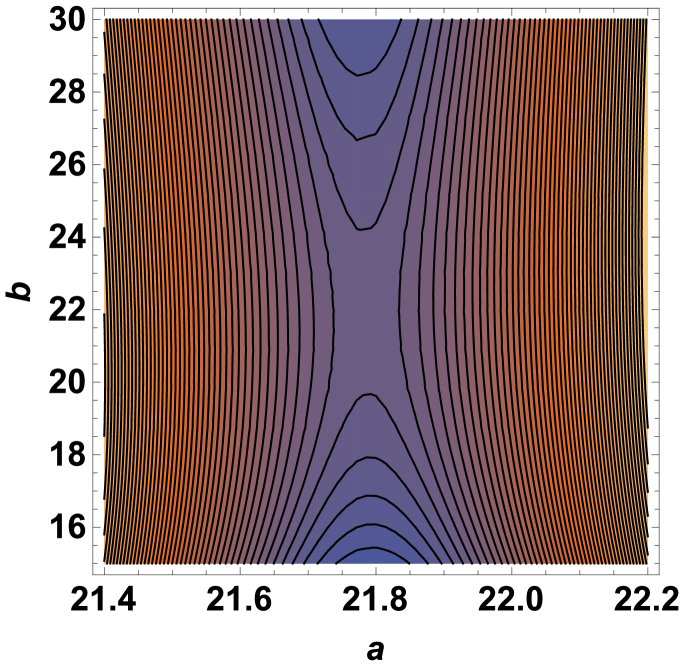
Figure 1: Energy contours for a reduced system in the Keplerian limit, where energy and angular momentum budgets include the planetary orbit, planetary spin, and lunar orbit. The critical point is a saddle point and occurs near the center of the diagram. The energy has a local minimum in the $a$-direction and a local maximum in the $b$-direction.

The existence of a saddle point arises because the system can transfer angular momentum between the lunar orbit and planetary orbit (and the planetary spin). To illustrate this behavior, we introduce a reduced system with only the two orbits and the planetary spin. The specific energy ${\cal E}=E/m$ takes the form

$${\cal E}=-{1\over 2a}-{\delta\over 2b}+{m\over 2}(\Lambda-\sqrt{a}-\delta\sqrt{b})^{2}\,,$$ (35)

where we have defined $\delta=\mu{m}^{-1/3}$ and $\Lambda=L/m$, and let $b\to{m^{-1/3}}b$. The contours of constant energy are shown in Figure 1 for one such system (where we have taken $\delta=10^{-3}$, $m=0.03$, and $\Lambda=5$. The energy has a critical point near the center of the diagram. The point is a minimum in the direction corresponding to variations in the planetary semimajor axis $a$, but is a local maximum in the orthogonal direction corresponding to variations in $b$.

2.3 Reduction to the Two-body System

As a consistency check, we consider the stability analysis in the limit where the moon mass is negligible by taking $\mu\to 0,K\to 0$, where we should recover the results found earlier for binary systems. In this limit, the three $4\times 4$ submatrices of the Hessian matrix reduce to three $2\times 2$ submatrices, with the variables $(a,\omega_{z})$ for $\mathbb{A}_{2}$, $(i,\omega_{x})$ for $\mathbb{B}_{2}$, and $(e,\omega_{y})$ for $\mathbb{C}_{2}$:

$$\mathbb{A}_{2}={m\over 4}\left[\matrix{a^{-3}(-3+ma^{2})&2Ja^{-1/2}\cr 2Ja^{-1/2}&4J(1+J)/m}\right],$$ (36)

$$\mathbb{B}_{2}=m\left[\matrix{a^{-1}(1+ma^{2})&a^{1/2}J\cr{a}^{1/2}J&J(1+J)/m}\right],$$ (37)

and

$$\mathbb{C}_{2}=\left[\matrix{m/a&0\cr 0&J(1+J)}\right].$$ (38)

It is straightforward to show that the eigenvalues of the reduced submatrices $\mathbb{B}_{2}$ and $\mathbb{C}_{2}$ are always positive. The conditions required for the reduced submatrix $\mathbb{A}_{2}$ to be positive definite take the forms

$${m}a^{2}>3\qquad{\rm and}\qquad ma^{2}>3(1+J).$$ (39)

The first condition is satisfied if the second one holds. The second condition can be rewritten in more suggestive form by converting back to physical units and rearranging to obtain $m(GMa)^{1/2}>3(I+J)\Omega$. In other words, the critical point is a minimum, and a tidal equilibrium state exists, provided that the orbital angular momentum is larger than three times the spin angular momentum of the system (consistent with previous results). Recall that in order for the critical point to exist, the total angular momentum must be larger than a minimum value $L_{X}$, given by equation (26). In the limit $\mu\to 0$, this lower bound becomes

$${L_{X}}={4\over 3}\left[3(I+J)m^{3}(GM)^{2}\right]^{1/4}.$$ (40)

3 Minimal Model Beyond the Keplerian Limit

This section takes the problem beyond the Keplerian approximation. The previous treatment did not include the tidal influence of the star on the lunar orbit or the fact that the lunar orbit resides in a rotating reference frame. These effects are included here by considering the circular restricted three-body problem (Szebehely, 1967) for the lunar orbit and by using an orbit-averaged approach (Goldreich, 1966). The results of this section are thus more useful for applications to real systems.

In this treatment, both the lunar orbit and the planetary orbit are taken to have no eccentricity. Motivated by the results of the previous section, we consider a reduced system where the energy and angular momentum budgets include only the planetary orbit, the lunar orbit, and the planetary spin. In particular, we ignore stellar rotation, so that this calculation applies to planetary orbits with semimajor axes large enough that the stellar angular momentum is decoupled. Finally, we assume that the angular momentum vectors of the two orbits and the planetary spin are aligned. With these specifications, the energy of the system (in dimensionless units where $G=M=J=1$) takes the form

$$E=-(m+\mu){1\over 2a}-{m\mu\over 2b}-\mu{b^{2}\over 2a^{3}}+{1\over 2}\omega^{2}\,.$$ (41)

The quantity $\omega$ = $\omega(a,b)$ is the rotation rate of the planet and is determined by conservation of angular momentum so that

$$\omega\equiv L-(m+\mu)\sqrt{a}-\mu\left[mb-b^{4}/2a^{3}\right]^{1/2}\,.$$ (42)

Equation (41) follows from an orbit-averaged approach (Goldreich, 1966) to the circular restricted three-body problem (Szebehely, 1967), whereas equation (42) makes the additional assumption that the orbit of the moon is also circular. Now we consider the specific energy ${\cal E}=E/m$ and ignore the difference between $m$ and $m+\mu$ for the planetary orbit. We also define the specific angular momentum $\Lambda=L/m$ and the ancillary quantity $\delta=\mu m^{-1/3}$. Finally, we rescale the radial variable for the lunar orbit $b\to m^{-1/3}b$. The specific energy can then be written in the form

$${\cal E}=-{1\over 2a}-{\delta\over 2b}-\delta{b^{2}\over 2a^{3}}+{m\over 2}(\Lambda-\sqrt{a}-\delta\left[b-b^{4}/2a^{3}\right]^{1/2})^{2}\,.$$ (43)

For future reference note that $\omega/m=\Lambda-\sqrt{a}-\delta\left[b-b^{4}/2a^{3}\right]^{1/2}$.

3.1 Equilibrium States: First Variation

Now we find the derivatives. The derivative for $a$ has the form

$${\partial{\cal E}\over\partial a}={1\over 2a^{2}}+{3\over 2}\delta{b^{2}\over{a^{4}}}-{\omega\over 2}\left\{a^{-1/2}+\delta\left[b-b^{4}/2a^{3}\right]^{-1/2}3b^{4}/2a^{4}\right\}\,.$$ (44)

The derivative for the second semimajor axis $b$ can be written

$${\partial{\cal E}\over\partial b}={\delta\over 2b^{2}}-\delta{b\over a^{3}}-{\delta\omega\over 2}\left[b-b^{4}/2a^{3}\right]^{-1/2}\left[1-2b^{3}/a^{3}\right]\,.$$ (45)

Setting the derivatives to zero we find

$$1+3\delta{b^{2}\over{a^{2}}}=\omega\left\{a^{3/2}+\delta\left[b-b^{4}/2a^{3}\right]^{-1/2}3b^{4}/2a^{2}\right\}\,,$$ (46)

and

$$\left[1-{2b^{3}\over a^{3}}\right]=\omega b^{2}\left[b-b^{4}/2a^{3}\right]^{-1/2}\left[1-{2b^{3}\over a^{3}}\right]\,.$$ (47)

The second relation has two solutions. The first solution implies

$$\omega^{2}={1\over b^{3}}-{1\over 2a^{3}}\qquad{\rm or}\qquad\eta^{2}=\omega^{2}+N^{2}/2\,.$$ (48)

At this critical point, the spin of the planet is synchronous with the orbital frequency of the moon (in the rotating frame of reference). The second solution implies

$${1\over b^{3}}={2\over a^{3}}\qquad{\rm or}\qquad\eta^{2}=2N^{2}\,.$$ (49)

This value of $b$ corresponds to the point where the orbital angular momentum of the moon has its maximum value.

The second critical point (where $\eta^{2}=2N^{2}$) will generally lie closer to the planet than the first critical point (where $\eta^{2}=\omega^{2}+N^{2}/2$). In order for the two critical points to coincide, the condition $\delta(b/a)^{2}=(-2+\sqrt{6})/3\approx 0.15$ must be met. As shown below, we expect $b/a\approx(2/3)^{1/3}$ at the critical point. (Recall that the semimajor axis $b$ is scaled by a factor of $m^{-1/3}$ so that $a$ and $b$ are comparable in size.) As a result, this condition implies $\delta\approx 0.2$. However, we expect $\delta$ to be small, more specifically $\delta=\mu m^{-1/3}\approx 10\mu\approx 10^{-4}\ll 1$, so the required condition is usually not satisfied for exomoons, and the first critical point (equation [48]) occurs farther from the planet than the second one (equation [49]).

3.2 Stability of the System: Second Variation

The second derivative for $a$ has the form

$${\partial^{2}{\cal E}\over\partial a^{2}}=-N^{2}-6\delta{b^{2}\over a^{2}}N^{2}+{\omega\over 4}N+{\omega\over 2}\delta\left\{\left[\eta^{2}-N^{2}/2\right]^{-1/2}6{b^{2}\over a^{2}}N^{2}+{9\over 8}\left[\eta^{2}-N^{2}/2\right]^{-3/2}{b^{2}\over a^{2}}N^{4}\right\}$$ (50)

$$+{ma^{2}\over 4}\left\{N+\delta\left[\eta^{2}-N^{2}/2\right]^{-1/2}(3b^{2}/2a^{2})N^{2}\right\}^{2}\,,$$

where we have used the definitions of $N$ and $\eta$ to simplify the expression. The mixed derivative is given by

$${\partial^{2}{\cal E}\over\partial b\partial a}={3\delta b\over a}N^{2}+\delta{\omega\over 2}\left\{-6\left[\eta^{2}-N^{2}/2\right]^{-1/2}+{3\over 4}\left[\eta^{2}-N^{2}/2\right]^{-3/2}\left[\eta^{2}-2N^{2}\right]\right\}{b\over a}N^{2}$$ (51)

$$+{m\delta\over 4}\left[\eta^{2}-N^{2}/2\right]^{-1/2}\left[\eta^{2}-2N^{2}\right]ab\left\{N+\delta[\eta^{2}-N^{2}/2]^{-1/2}(3b^{2}/2a^{2})N^{2}\right\}\,.$$

The second derivative with respect to $b$ has the form

$${\partial^{2}{\cal E}\over\partial b^{2}}=-\delta\eta^{2}-\delta N^{2}+{m\delta^{2}b^{2}\over 4}\left[\eta^{2}-N^{2}/2\right]^{-1}\left[\eta^{2}-2N^{2}\right]^{2}$$ (52)

$$+\delta{\omega\over 2}\left\{6N^{2}\left[\eta^{2}-N^{2}/2\right]^{-1/2}+{1\over 2}\left[\eta^{2}-N^{2}/2\right]^{-3/2}\left[\eta^{2}-2N^{2}\right]^{2}\right\}\,.$$

To simplify the expressions for the second derivatives, we define the following quantities:

$$\lambda=\left[\eta^{2}-N^{2}/2\right]^{1/2},\qquad A=\eta^{2}-2N^{2},\qquad{\rm and}\qquad\xi=\delta{b^{2}\over a^{2}}\,.$$ (53)

The conditions for the first derivatives to vanish then become

$$\lambda=\omega\qquad{\rm and/or}\qquad A=0\,,$$ (54)

for the derivative with respect to $b$, and

$$1+3\xi=\omega\left\{{1\over N}+{3\xi\over 2\lambda}\right\}\,$$ (55)

for the derivative with respect to $a$. If we also divide by $N^{2}$, the second derivatives simplify as follows:

$${\cal E}_{aa}=-1-6\xi+{\omega\over 4N}+\omega{\xi\over\lambda}\left\{3+{9\over 16}{N^{2}\over\lambda^{2}}\right\}+{ma^{2}\over 4}\left\{1+{3\over 2}\xi{N\over\lambda}\right\}^{2}\,,$$ (56)

$${\cal E}_{ab}={3\delta b\over a}+{3\delta\omega\over\lambda}\left\{-1+{A\over 8\lambda^{2}}\right\}{b\over a}+{m\delta ab\over 4}{A\over N\lambda}\left\{1+{3\over 2}\xi{N\over\lambda}\right\}\,,$$ (57)

and

$${\cal E}_{bb}=-\delta{\eta^{2}\over N^{2}}-\delta+{m\delta^{2}b^{2}\over 4}{A^{2}\over N^{2}\lambda^{2}}+{\delta\omega\over\lambda}\left\{3+{A^{2}\over 4N^{2}\lambda^{2}}\right\}\,.$$ (58)

3.3 Critical Point for Lunar Orbit with Maximum Angular Momentum

Now we invoke the critical point condition $\eta^{2}=2N^{2}$ so that $A=0$. This condition corresponds to the case where the lunar orbit has its maximum angular momentum. The second derivatives, when evaluated at the critical point, represent the elements of the Hessian matrix, which become:

$${\cal E}_{aa}=-1-6\xi+{\omega\over 4N}+\omega{\xi\over\lambda}\left\{3+{9\over 16}{N^{2}\over\lambda^{2}}\right\}+{ma^{2}\over 4}\left\{1+{3\over 2}\xi{N\over\lambda}\right\}^{2}\,,$$ (59)

$${\cal E}_{ab}=3\delta{b\over a}\left[1-{\omega\over\lambda}\right]\,,$$ (60)

and

$${\cal E}_{bb}=-3\delta\left[1-{\omega\over\lambda}\right]\,.$$ (61)

To determine if the critical point is a minimum, we evalute the minors of the Hessian matrix. Let us define

$$\alpha={\cal E}_{aa}\qquad{\rm and}\qquad\beta=3\delta\left[1-{\omega\over\lambda}\right]\,,$$ (62)

so that

$${\cal E}_{bb}=-\beta\qquad{\rm and}\qquad{\cal E}_{ab}={b\over a}\beta\,.$$ (63)

The conditions for the minors to be positive then take the forms

$$\alpha>0\qquad{\rm and}\qquad-\alpha\beta>{b^{2}\over a^{2}}\beta^{2}\,.$$ (64)

These conditions thus require $\beta<0$ so that $\omega>\lambda$. However, since $\eta^{2}=2N^{2}$, the parameter $\lambda=(3/2)^{1/2}N$ and equation (55) implies that

$${\omega\over\lambda}=\left({2\over 3}\right)^{1/2}{1+3\xi\over 1+(3/2)^{1/2}\xi}\,.$$ (65)

The leading factor is less than unity, whereas the second factor is of order unity, so that $\omega<\lambda$ and hence $\beta>0$. In fact, the right hand side approaches unity only in the limit $\xi\to\infty$, so that the factor is less than unity for any physical values of the parameters. As a result, the required condition cannot be satisfied, the minors cannot both be positive, and the critical point is not a minimum.

3.4 Critical Point for Co-rotating Lunar Orbit

We now consider the critical point where $\lambda=\omega$, which corresponds to the case where the planetary rotation rate and the mean motion of the lunar orbit are synchronous in the rotating frame of reference. This condition follows from setting the derivative of the energy with respect to $b$ equal to zero. The corresponding condition for the derivative with respect to $a$ implies

$$\lambda=N\left[1+{3\over 2}\xi\right]=fN\,.$$ (66)

We also have the relations

$$\eta^{2}=(f^{2}+1/2)N^{2}\qquad{\rm and}\qquad A=(f^{2}-3/2)N^{2}\,.$$ (67)

Using these results, the second derivatives (matric elements) become

$${\cal E}_{aa}=-1+{f\over 4}+3\xi\left\{-1+{3\over 16f^{2}}\right\}+{ma^{2}\over 4}\left\{1+{3\over 2}{\xi\over f}\right\}^{2}\,,$$ (68)

$${\cal E}_{ab}={3\delta b\over a}{f^{2}-3/2\over 8f^{2}}+{m\delta\over 4}{(f^{2}-3/2)ab\over f}\left\{1+{3\over 2}{\xi\over f}\right\}\,,$$ (69)

and

$${\cal E}_{bb}=\delta(3/2-f^{2})+\delta(1+m\delta b^{2}){(f^{2}-3/2)^{2}\over 4f^{2}}\,.$$ (70)

To fix ideas, let’s evaluate the matrix elements in the extreme limit where $\delta,\xi\to 0$. Keeping only leading order terms, we find:

$${\cal E}_{aa}={1\over 4}(ma^{2}-3)\,,\quad{\cal E}_{ab}=-{\delta\over 16}{b\over a}(3+2ma^{2})\,,\quad{\rm and}\quad{\cal E}_{bb}={9\delta\over 16}\,.$$ (71)

The condition for the first minor to be positive is simply

$$ma^{2}>3\,,$$ (72)

whereas the condition for the second minor to be positive is

$$9(ma^{2}-3)>{\delta\over 4}{b^{2}\over a^{2}}(3+2ma^{2})^{2}\,,$$ (73)

which can be rewritten in the form

$$ma^{2}>3+\xi\left[{1\over 4}+{1\over 3}ma^{2}+{1\over 9}(ma^{2})^{2}\right]\,.$$ (74)

Since we expect $\xi\sim\delta\ll 1$, the constraint required for the second minor to be positive is only slightly more restrictive than the condition required for the first minor to be positive.

Now let’s look at the conditions required for this critical point to exist. At the critical point, the rotation frequency is given by

$$\omega^{2}={1\over b^{3}}-{1\over 2a^{3}}\,,$$ (75)

which comes from the condition that the $b$-derivative vanishes. The requirement that $a$-derivative vanishes implies that

$$\omega=a^{-3/2}\left[1+{3\over 2}\delta{b^{2}\over a^{2}}\right]\,,$$ (76)

and finally we have the definition of $\omega$ in terms of the total angular momentum

$$\omega=m\left[\Lambda-a^{1/2}-\delta b^{2}\omega\right]\,.$$ (77)

We thus have three equations for the three unknowns $(\omega,a,b)$. We can combine the first two equations, by eliminating $\omega$, to obtain

$$\left[1+{3\over 2}\delta{b^{2}\over a^{2}}\right]^{2}={a^{3}\over b^{3}}-{1\over 2}\,.$$ (78)

Let $x=b/a$ so that we obtain

$${3\over 2}+3\delta x^{2}+{9\over 4}\delta^{2}x^{4}={1\over x^{3}}\,.$$ (79)

This equation always has one (and only one) positive real solution for $x=b/a$ for a given value of the mass parameter $\delta$. We can thus take $x$ to be specified. The remaining equation implies that

$$L=m\Lambda=ma^{1/2}+(1+m\delta x^{2}a^{2})a^{-3/2}\left[1+{3\over 2}\delta x^{2}\right]\,,$$ (80)

which can be rearranged to the form

$$L=ma^{1/2}\left[1+\delta x^{2}+{3\over 2}\delta^{2}x^{4}\right]+\left[1+{3\over 2}\delta x^{2}\right]a^{-3/2}\,,$$ (81)

The angular momentum $L$ of the system must exceed a minimum value $L_{X}$ in order for this equation to have a real solution, where the minimum is given by

$$L_{X}={4\over 3}\left\{{3\over m}\left[1+{3\over 2}\delta x^{2}\right]\left[1+\delta x^{2}+{3\over 2}\delta^{2}x^{4}\right]^{3}\right\}^{1/4}\,.$$ (82)

In physical units, the minimum value of the angular momentum has the form

$$L_{X}={4\over 3}\left[3JG^{2}M^{2}m^{3}\left(1+{3\over 2}\delta x^{2}\right)\left(1+\delta x^{2}+{3\over 2}\delta^{2}x^{4}\right)^{3}\right]^{1/4}\,.$$ (83)

In this expression, the dimensionless composite parameter $\delta{x^{2}}=(\mu{b^{2}})/(ma^{2})$, where $a$ and $b$ are now in physical units, and where the ratio $b/a$ is determined by the solution to equation (79). For this minimum value $L_{X}$, the combined angular momentum of the orbits (both the planet and moon) is three times that of the planetary spin. Recall that in the previous case of two-body systems (Hut, 1980), the orbital angular momentum of the binary had to be larger than three times the spin angular momentum for the stable equilibrium point to exist. Three-body systems thus produce a similar result, where the two contributions to the orbital angular momentum act together in the accounting.

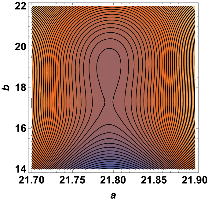
Figure 2: Energy contours for a reduced system including stellar interactions with the lunar orbit. The energy and angular momentum budgets include the planetary orbit, planetary spin, and lunar orbit. The critical point is a minimum, so that a stable tidal equilibrium state exists for the system.

We thus expect this second critical point to be a minimum, provided that the total angular momentum of the system exceeds that mininmum given by equation (82). Figure 2 depicts a contour plot of the energy for the model system with parameters $\Lambda=5$, $\delta=10^{-3}$, and $m=0.03$ (the same as those used in constructing Figure 1). With the generalized treatment of the lunar orbit, the system has two critical points, where the first is a saddle point and the second is a minimum. As a result, a stable tidal equilibrium state exists for the system.

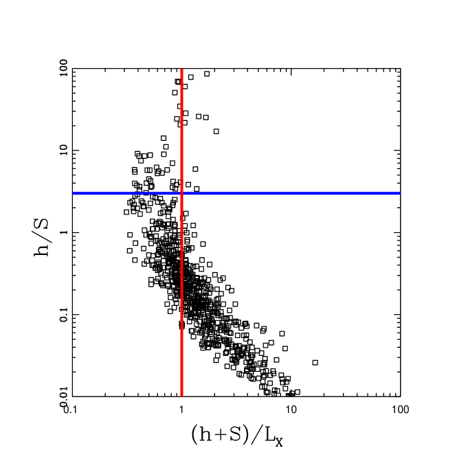
Figure 3: Angular momentum variables for a collection of observed extrasolar planetary systems, where $h$ is the orbital angular momentum and $S$ is the rotational angular momentum of the star. The horizontal axis shows the ratio of total angular momentum to the minimum value $L_{X}$ required for tidal equilibrium states to exist. The vertical axis shows the ratio of the orbital to spin angular momentum. Only systems that fall to the right of the vertical red line and above the horizontal blue line can have stable tidal equilibrium states.

Although a stable tidal equilibrium state can exist, its location is essentially at the co-rotation point, which is close to the Hill radius. For comparison, a large body of numerical work suggests that lunar orbits cannot remain stable over long spans of time if their orbits are larger than about half the Hill radius (for further discussion, see Szebehely 1978; Barnes & O’Brien 2002; Domingos et al. 2006; Donnison 2010; Payne et al. 2013, and references therein). In other words, lunar orbits corresponding to the tidal equilibrium point are rendered unstable by dynamical interactions, so that the tidal equilibrium point found here does not represent a viable long-term state of the system.

The fact that the tidal equilibrium point occurs near the Hill radius can be understood as follows: At the Hill radius, the lunar orbit has nearly the same frequency as the planetary orbit (because the tidal force due to the star and the gravitational force of the planet act nearly equally on the moon). Tidal equilibrium for the star-planet system requires the stellar spin and the planetary spin to coincide with the orbital frequency of the planet (for further detail, see Hut 1980). Similarly, tidal equilibrium for the planet-moon system requires the planetary spin to coincide with the orbital frequency of the moon. For the combined star-planet-moon system, in equilibrium, the orbital frequencies must match up with the spin frequencies, so that both orbits must have the same period. This matching of the periods thus leads to the tidal equilibrium point being near the Hill radius, even though the latter does not involve rotation rates of the three bodies.

4 Application to Observed Extrasolar Planetary Systems

The results of the previous sections outline the properties necessary for star-planet-moon systems to have stable tidal equilibrium states. As outlined above, such equilibrium states lie outside the boundary — half the Hill radius — where dynamical scattering is expected to compromise lunar orbits. Moreover, with no detections of exomoons to date, we cannot (yet) make a full assessment of the relationship between exomoon orbits and those corresponding to tidal equilibrium states in observed extrasolar planetary systems. Nonetheless, existing data can be used to place constraints. In this section, we first consider star-planet systems without moons and show that they generally cannot have stable tidal equilibrium states. We then find that hypothetical moons in such systems could have stable tidal equilibrium states, provided that the star-planet systems have stable states. Finally, we consider the largest moons in our Solar System and find that their orbits fall far inside the location of both the tidal equilibrium state and the dynamical stability boundary.

The results from Section 2.3 outline the properties necessary for the star-planet system (without a moon) to have a stable tidal equilibrium state (equations [39] and [40]). Using these results, consistent with previous findings (Hut, 1980; Adams & Bloch, 2015), we can determine whether extrasolar planet candidates in the current sample meet the criteria for stability. Here we consider the innermost planets discovered by the Kepler mission (Batalha et al., 2013). Since we also need to know the stellar rotation rates in order to evaluate the stability conditions, we consider a subset of the sample where the host stars have measured rotation periods (McQuillan et al., 2013). After removing eclipsing binaries and other non-planetary systems, we are left with 738 systems with detected planets and measured stellar periods. The planets in these systems primarily have masses in the range $m$ = few – 30 $M_{\oplus}$ (only 30 planets in the sample have mass $m>0.5m_{J}$). Note that we are assuming that the planetary candidates are real and that their observed radii and inferred orbital elements are accurate.

In order to convert the observed radius measurements $R_{p}$ to planetary mass estimates, we use the scaling relationship $m$ = $M_{\earth}(R_{p}/R_{\earth})^{2.1}$ (Lissauer et al., 2011). For most of the sample, the orbital eccentricities are not detectable, and they are set to zero for this analysis. We also need to specify the moment of inertia for the host stars, which can be written in the form $I=\chi M_{\ast}R_{\ast}^{2}$. For simplicity we take $\chi=0.10$, a value that is intermediate between polytopes with indices $n=3/2$ and $n=3$ (e.g., see Batygin & Adams 2013). The benchmark value of the angular momentum depends on the moment of inertia according to $L_{X}\propto I^{1/4}$, so that the results do not depend sensitively on this choice.

Subject to the assumptions outlined above, we calculate the orbital angular momentum $h=m(GMa)^{1/2}$ of the planet and the spin angular momentum $S=I\Omega$ of the host star. Figure 3 shows the ratio of $h/S$ plotted versus the ratio $(h+S)/L_{X}$, where $L_{X}$ is the minimum angular momentum for two-body systems from equation (40). In order for any tidal equilibrium state to exist for the star-planet system, the total angular momentum must exceed the critical value $L_{X}$. This condition $h+S>L_{X}$ is shown by the vertical red line in the figure. In order for the tidal equilibrium state to be a minimum, and hence stable, the orbital angular momentum must be larger than three times the spin angular momentum. This condition, $h/S=3$, is depicted by the horizontal blue line in the figure. Only those systems that satisfy both criteria can have stable tidal equilibrium states. As shown by the points in the upper right quadrant of Figure 3, only 11 (out of the original 738) systems meet both stability conditions. The majority of systems either have no tidal equilbrium state or do not have enough orbital angular momentum for the equilibrium state to be stable (a sizable fraction of the systems fail to meet either constraint).

Most of these systems are not old enough to have reached a stable tidal equilibrium state (if it exists) or to have lost their planet (if it does not). Of the 738 planets in the sample, only 239 have semimajor axes $a<0.05$ AU (and 491 have $a<0.10$ AU), so that the majority of the planets are effectively decoupled from their stars. As a result, the time scales for tidal evolution (Hut, 1981; Zahn, 1977) are longer than the ages of the systems (Walkowicz & Basri, 2013).

We now consider hypothetical moons in orbit about the planets in the sample. The results from Section 3 consider the star-planet-moon system in the absence of stellar rotation and find the angular minimum angular momentum $L_{X}$ necessary for a tidal equilibrium state to exist (see equation [83]). Keep in mind that this value of $L_{X}$ for the star-planet-moon system is not the same as the minimum value necessary for the two-body system. Since the total angular momentum must be larger than $L_{X}$, a sufficient condition is for the planetary orbital angular momentum to exceed this value. We thus require

$$m(GMa)^{1/2}>L_{X}={4\over 3}\left[3JG^{2}M^{2}m^{3}\left(1+{3\over 2}\delta x^{2}\right)\left(1+\delta x^{2}+{3\over 2}\delta^{2}x^{4}\right)^{3}\right]^{1/4}\,,$$ (84)

which reduces to the constraint

$$ma^{2}>{256J\over 27}\left(1+{3\over 2}\delta x^{2}\right)\left(1+\delta x^{2}+{3\over 2}\delta^{2}x^{4}\right)^{3}\approx{256\over 27}mR_{p}^{2}\,,$$ (85)

where $R_{p}$ is the radius of the planet. In obtaining the final approximate constraint, we assume that the parameter combination $\delta x^{2}={\cal O}(\mu/M)$ is small. We thus obtain the (sufficient) condition $a\raise 1.29167pt\hbox{$>$}\kern-7.5pt\lower 3.01385pt\hbox{$\sim$}3.08R_{p}$. Since planets are usually smaller than their host stars by an order of magnitude ($R_{\ast}\sim 10R_{p}$) and the planetary orbit must lie outside the star ($a>R_{\ast}$) this condition is always satisfied. As a result, the star-planet-moon systems will (almost always) have stable tidal equilibrium states, provided that the star-planet subsystems have stable tidal equilibrium states. Of course, as discussed previously, moons orbiting at the equilibrium locations are susceptible to dynamical scattering.

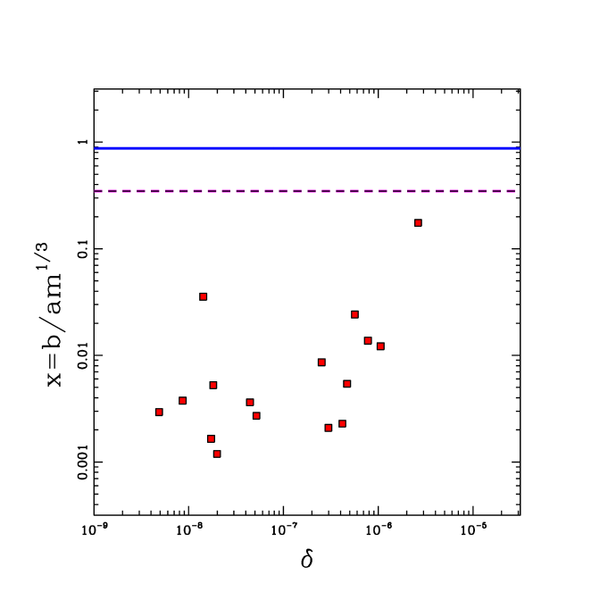
Figure 4: Scaled orbital ratios for the largest moons in our Solar System, plotted versus the scaled mass parameter $\delta$. The upper blue curve marks the location of the stable tidal equilibrium point. The dashed magenta line marks the location of half the Hill radius, which represents the widest orbit that is expected to be stable according to previous numerical simulations. The points correspond to the 16 largest moons in our Solar System.

Next we apply the results of this analysis to the moons of our own Solar System. Here we consider the 16 largest moons of the Solar System. These bodies orbit Earth (our moon), Pluto (Charon), and the four giant planets. For a given moon mass $\mu$ and planetary mass $m$, we calculate the mass parameter $\delta=\mu/m^{1/3}$, where the masses have been scaled by the mass of Sun. The solution to equation (79) then determines the location of the stable tidal equilibrium point for the moon in terms of the ratio $b/(am^{1/3})$. This orbital ratio can then be compared to those of observed moons.

Figure 4 shows the observed values (red points) of the scaled orbital ratio as a function of the mass parameter $\delta$ for the largest moons in our Solar System. The dashed magenta line shows the location where the moons would orbit at half their Hill radius. Numerical simulations (Payne et al., 2013) indicate that moons with larger orbits (above the magenta line) are susceptible to being dynamically removed from their host planets, so that we do not expect any points to fall above this line. For comparison, the solid blue curve shows the value of the orbital ratio corresponding to the stable tidal equilibrium point (from Section 3). Note that the curve is nearly constant, as expected for the small values of $\delta$ realized within the Solar System. More importantly, the tidal equilibrium point (solid blue curve) lies outside the stability boundary (dashed magenta line). This ordering implies that the conditions for a stable tidal equilibrium state are at odds with the requirement for dynamical stability indicated by numerical simulations.

In Figure 4, the point with the largest mass parameter $\delta$ and the largest orbital ratio (in the upper right part of the diagram) corresponds to our Moon. The other point that stands out in the figure is the relatively large orbital ratio for the moon Iapetus, which orbits Saturn. Except our Moon, Iapetus orbits farther from its host planet than other (large) moons in our system. With the exception of the Pluto-Charon system, all of the moons have orbital periods that are larger than the planetary rotation periods. Because the planets are spinning faster, tidal forces on the moons are expected to move them outward toward instability (upward in Figure 4). In contrast, Pluto and Charon and mutually tidally locked. The rotational periods of Pluto and Charon, as well as their orbital period, are all about 6.4 days. If considered in isolation from the Sun, the Pluto-Charon system is thus in a stable equilibrium state for two-body systems (in addition to synchronicity, the total angular momentum of the system and the faction of orbital angular momentum are large enough). However, Figure 4 indicates that the three-body system Sun-Pluto-Charon is not in a stable tidal equilibrium state. The system could evolve to a lower energy state by transferring angular momentum to its orbit about the Sun.

5 Conclusion

This paper considers the issue of tidal equilibrium for hierarchical star-planet-moon systems, which are described by 16 variables that specify the energy and angular momentum of the stellar spin, planetary spin, planetary orbit, lunar orbit, and lunar spin. The optimization procedure is subject to the constraint of constant angular momentum. A summary of our results is given below, along with a discussion of their implications.

5.1 Summary of Results

The first finding of this paper is that stable tidal equilibrium states do not exist for hierarchical star-planet-moon systems for the case where orbits are described in the Keplerian limit (Section 2). This result stands in contrast to case of binary systems with spin angular momentum, also evaluated in the Keplerian limit, where stable tidal equilibrium states are present as long as the total angular momentum of the system is sufficiently large. In the Keplerian approximation, the system energy has a single critical point which corresponds to synchronous rotation of the star, planet, moon, planetary orbit, and the lunar orbit. In addition, both orbits have zero eccentricity and all five angular momentum vectors are aligned. However, the critical point does not represent a minimum of the energy, but rather a saddle point (Figure 1). Moreover, at the critical point, the lunar orbit lies outside the Hill radius, although this boundary is not defined within the Keplerian approximation.

In practice, this finding indicates that the system can evolve to a lower energy state — while conserving total angular momentum — by changing the orbital radius of the moon from its critical value. If the moon moves inward toward the planet, orbital angular momentum of the lunar orbit decreases, and the spin and/or the orbital angular momentum of the planet must increase to compensate. If the moon moves outward and increases its orbital angular momentum, the spin and/or orbital angular momentum of the planet decrease accordingly.

In the Keplerian limit, the formulation does not include the tidal force from the star acting on the lunar orbit. This interaction term specifies the Hill radius, which provides an effective outer boundary for allowed lunar orbits. One can include this effect in the formulation, provided that the additional terms are time-averaged. We have generalized the calculation so that the lunar orbit is treated using the circular restricted three-body approximation (Section 3). In this case, the energy of the system has two critical points. The first is a saddle point, whereas the second one is a local minimum (Figure 2). As a result, a stable tidal equilibrium state exists for this system. The existence of the tidal equilibrium state requires that the total angular momentum of the system exceeds a well-defined value $L_{X}$ (given by equation [82]), analogous to results obtained previously for binary systems. For $L=L_{X}$, the combined orbital angular momentum of both orbits is three times the rotational angular momentum of the planet. Even when it exists, the stable tidal equilibrium point lies outside the boundary (roughly half the Hill radius) where lunar orbits are found to be stable in numerical simulations. As a result, the tidal equilibrium point found here does not does not represent a viable long-term state of the system.

Although exomoon systems can in principle have stable tidal equilibrium states, most observed systems with exo-jupiters don’t have the right angular momentum for a stable tidal equilibrium state to exist even for the star-planet system considered without a moon (as illustrated by Figure 3). For host stars with measured stellar rotation rates (McQuillan et al., 2013), the total angular momentum is generally less than the critical value $L<L_{X}$ and/or the orbital angular momentum is too small relative to the total (see also Levrard et al. 2009; Adams & Bloch 2015). Since these star-planet systems do not reside in tidal equilibrium, existing systems must dissipate energy and evolve. However, the time scales must be longer than typical system ages (several Gyr), and this requirement places constraints on the tidal dissipation parameters. In a similar vein, moons in our Solar System orbit much closer to their host planets than both the tidal equilibrium point and the dynamical stability boundary (Figure 4). Although these moons will eventually be exiled as they gain orbital angular momentum from their host planets, they remain in orbit because the Solar System is not old enough for this process to proceed to completion.

5.2 Discussion

The problem of finding tidal equilibrium states for hierarchical three-body systems is well-defined in principle. However, the application of these results to astronomical systems requires further discussion. First we note that although the full three-body problem has energy and angular momentum integrals (Sundman, 1913), the expressions used here for these conserved quantities are necessarily approximate. Because the planetary orbit is nearly Keplerian, the key approximation in this study is the model used to describe the lunar orbit. In general, the angular momentum of the moon (in orbit about the planet) is not constant in time. However, in both the Keplerian limit (Section 2) and the restricted three-body generalization used here (Section 3), the time-averaged lunar orbit does have well-defined angular momentum integral (e.g., see Goldreich 1966). As a result, the constrained optimization procedure of this paper is valid in a time-averaged sense. Since moons are expected to have periods $P\sim 1-100d$, whereas evolutionary times scales are $\sim$Gyr, the time-averaged angular momentum of the lunar orbit is indeed well-defined for the time scales over which the system energy is expected to change.

Another issue that arises is the long-term dynamical stability of star-planet-moon systems. In the Keplerian limit, the critical point lies outside the Hill radius, and the critical point is a saddle point, so that no chance of stability arises. In the orbit-averaged case (Section 3), the potentially stable critical point lies near the Hill radius that one obtains for the time-averaged problem, and the critical point can be a minimum. However, numerical simulations show that the stability of lunar orbits requires the semimajor axis to be less than a fraction (typically $f\sim 1/2)$ of the standard Hill radius (Payne et al. 2013 and references therein). In scaled units ($G=M=J=1$ and $b\to{b}m^{-1/3}$), this requirement becomes $b/a<1/(2\cdot 3^{1/3})$. In contrast, the value of the ratio $b/a$ at the stable equilibrium point is given by the solution to equation (79), which implies $b/a\approx(2/3)^{1/3}$. The two locations differ by a factor of $2^{4/3}\approx 2.52$. The dynamical stability constraint thus requires the moon to orbit well inside the critical point found here. Such systems can evolve to lower energy states by decreasing the lunar semimajor axis and transferring angular momentum to the planetary orbit and/or the planetary rotational energy.

Although star-planet-moon systems often have no stable tidal equilibrium states, the moons in our Solar System exist over Gyr time scales as they evolve (Goldreich & Soter, 1966). Possible moons in other systems can have shorter lifetimes (Barnes & O’Brien, 2002). Tidal forces act to move the moons outward (inward) if the planetary rotation rate is larger (smaller) than the orbital mean motion. For systems that are dynamically stable, moons must orbit well within the Hill sphere. Since the planetary spin is close to synchronous with the planetary orbit for systems near the critical point, which is near the Hill radius, the lunar mean motion will generally be larger than the planetary spin; in this case, the moon will eventually fall into the planet. For systems residing far from their critical point, however, the planet rotation rate could be super-synchronous, so that the lunar orbit evolves outward and the moon eventually becomes unbound from the planet.

We also note that the tidal equilibrium states considered in this paper are related to spin-orbit resonances. Many of the moons in our Solar System are in or near a synchronous spin-orbit resonance where the orbital period of the moon is commensurate with the rotational period of the planet (Murray & Dermott, 1999). These configurations correspond to minimum energy states and planet-moon systems are driven toward such states through the action of dissipative forces. Tidal equilibrium states are also minimum energy configurations. In practice, planet-moon systems in spin-orbit resonance undergo small oscillations about the equilibrium state. In addition, the full description of the equilibrium state includes additional properties of the system, such as the quadrupole moments of the bodies (see Chapter 5 of Murray & Dermott 1999).

This paper has only considered the energy states of these hierarchical systems, and not the dynamical evolution toward the equilibrium states. This evolution must take place through dissipative processes such as tidal interaction between the constituent bodies. We note that the time scales for such interactions will generally be different for the star-planet system and the planet-moon system. As a result, one of the two-body subsystems can reach its tidal equilibrium state while the three-body system as a whole remains far from its tidal equilibrium state. In our Solar System, the Sun-Pluto-Charon system provides one such example.

The results of this paper change our interpretation of star-planet-moon systems: Lunar orbits in these systems, including our own Solar System, often have no tidal equilibrium states and cannot be absolutely stable (and this result stands in contrast to the case of two-body systems). When stable tidal equilibrium states exist, the required lunar orbits are so distant that dynamical interactions render the systems untenable, so that the moons can be scattered out of their orbits. If moons orbit close enough to their host planets to avoid this fate, they must lie well inside any possible stable equilibrium point, and must evolve through the action of dissipative forces (perhaps on long time scales). As a result, lunar orbits can only persist because the systems are not old enough for them to have dissipated their energy, or for dynamical interactions to scatter the moons out of their planet-centric orbits.

Acknowledgments: We thank Konstantin Batygin, Juliette Becker, Seth Jacobson, Dan Scheeres and Chris Spalding for useful conversations. We also thank an anonymous referee for useful comments.

References

- Adams & Bloch (2015) Adams, F. C., & Bloch, A. M. 2015, MNRAS, 446, 3676
- Agol et al. (2005) Agol, E., Steffen, J., Sari, R., & Clarkson, W. 2005, MNRAS, 359, 567
- Barnes & O’Brien (2002) Barnes, J. W., & O’Brien, D. P. 2002, ApJ, 575, 1087
- Batalha et al. (2013) Batalha, N. M., Rowe, J. F., Bryson, S. T., et al. 2013, ApJS, 204, 24
- Batygin & Adams (2013) Batygin, K., & Adams, F. C. 2013, ApJ, 778, 169
- Counselman (1973) Counselman, C. C. 1973, ApJ, 180, 307
- Darwin (1879) Darwin, G. H. 1879, The Observatory, 3, 79
- Darwin (1880) Darwin, G. H. 1880, Phil. Trans. R. Soc. A, 171, 713
- Domingos et al. (2006) Domingos, R. C., Winter, O. C., & Yokoyama, T. 2006, MNRAS, 373, 1227
- Donnison (2010) Donnison, J. R. 2010, MNRAS, 406, 1918
- Georgakarakos (2008) Georgakarakos, N. 2008, CeMDA, 100, 151
- Gilbert (1991) Gilbert, G. T. 1991, Amer. Math. Monthly, 98, 44
- Goldreich (1966) Goldreich, P. M. 1966, MNRAS, 4, 411
- Goldreich & Peale (1966) Goldreich, P. M., & Peale, S. 1966, MNRAS, 71, 425
- Goldreich & Soter (1966) Goldreich, P. M., & Soter, S. 1966, Icarus, 5, 375
- Heller et al. (2014) Heller, R., Williams, D., Kipping, D., et al. 2014, AstroBio, 14, 798
- Hesse (1872) Hesse, L. O. 1872, Die Determinanten elementar behandelt (Leipzig)
- Holman & Murray (2005) Holman, M. J., & Murray, N. W. 2005, Science, 307, 1288
- Hut (1980) Hut, P. 1980, A&A, 92, 167
- Hut (1981) Hut, P. 1981, A&A, 99, 126
- Jacobson & Scheeres (2011) Jacobson, S. A., & Scheeres, D. J. 2011, ApJ, 736, 19
- Kasting et al. (1993) Kasting, J. F., Whitmire, D. P., & Reynolds, R. T. 1993, Icarus, 101, 108
- Kipping (2009) Kipping, D. M. 2009, MNRAS, 392, 181
- Kipping et al. (2009) Kipping, D. M., Fossey, S. J., & Campanella, G. 2009, MNRAS, 400, 398
- Levrard et al. (2009) Levrard, B., Winisdoerffer, C., & Chabrier, G. 2009, ApJ, 692, 9
- Lissauer et al. (2011) Lissauer, J. J., Ragozzine, D., Fabrycky, D. C. et al. 2001, ApJS, 197, 8
- Matsumura et al. (2010) Matsumura, S., Peale, S. J., & Rasio, F. A. 2010, ApJ, 725, 1995
- McQuillan et al. (2013) McQuillan, A., Mazeh T., & Aigrain S. 2013, ApJ, 775, 11
- Murray & Dermott (1999) Murray, C. D., & Dermott, S. F.1999, Solar System Dynamics (Cambridge: Cambridge Univ. Press)
- Payne et al. (2013) Payne, M. J., Deck, K. M., Holman, M. J., & Perets, H. B. 2013, ApJ, 775, 44
- Spalding et al. (2016) Spalding, C., Batygin, K., & Adams, F. C. 2016, ApJ, 817, 18
- Sundman (1913) Sundman, K. F. 1913, Acta Math., 36, 105
- Szebehely (1967) Szebehely, V. 1967, Theory of Orbits: The restricted problem of three bodies (New York: Academic Press)
- Szebehely (1978) Szebehely, V. 1978, Cel. Mech., 18, 383
- Tholen et al. (1987) Tholen, D. J., Buie, M. W., Binzel, R. P., Frueh, M. L. 1987, Science, 237, 512
- Touma & Wisdom (1994) Touma, J., & Wisdom, J. 1994, AJ, 108, 1943
- Walkowicz & Basri (2013) Walkowicz, L. M., & Basri, G. S. 2013, MNRAS, 436, 1883
- Weidner & Horne (2010) Weidner, C., & Horne, K. 2010, A&A, 521A, 76
- Zahn (1977) Zahn, J. P. 1977, A&A, 41, 329