Bayesian modelling for binary outcomes in the Regression Discontinuity Design

Abstract

The Regression Discontinuity (RD) design is a quasi-experimental design which emulates a randomised study by exploiting situations where treatment is assigned according to a continuous variable as is common in many drug treatment guidelines.

The RD design literature focuses principally on continuous outcomes. In this paper we exploit the link between the RD design and instrumental variables to obtain a causal effect estimator, the risk ratio for the treated (RRT), for the RD design when the outcome is binary.

Occasionally the RRT estimator can give negative lower confindence bounds. In the Bayesian framework we impose prior constraints that prevent this from happening. This is novel and cannot be easily reproduced in a frequentist framework.

We compare our estimators to those based on estimating equation and generalized methods of moments methods. Based on extensive simulations our methods compare favourably with both methods.

We apply our method on a real example to estimate the effect of statins on the probability of Low-density Lipoprotein (LDL) cholesterol levels reaching recommended levels.

Keywords: risk ratio for the treated, prior constraints, causal effect

1 Introduction

The Regression Discontinuity (RD) design is a quasi-experimental design introduced in the 1960’s in Thistlethwaite and Campbell (1960) and widely used in economics and related social sciences (Imbens and Lemieux (2008)) and more recently in the medical sciences (Geneletti et al. (2015); Bor et al. (2014)). The RD design enables use of routinely gathered medical data from general practice (family doctors) to evaluate the causal effects of drugs prescribed according to well-defined decision rules. Most of the RD design literature focuses on continuous outcomes. Here we develop Bayesian approach for binary outcomes which are frequently of primary interest in health care contexts.

The RD design naturally leads to an Instrumental Variable (IV) analysis and so we adapt the IV based Multiplicative Structural Mean Model (MSMM) Risk Ratio for the Treated (RTT) estimator (Clarke and Windmeijer (2012, 2010); Hernan and Robins (2006)) to this context. The RRT is a measure of the change in risk for those who received the treatment. The MSMM estimator for the RRT is known to occasionally misbehave in that lower 95% confidence intervals can be negative (Clarke and Windmeijer (2010)). It is possible that this is why this estimator is not widely used despite its relatively simple formulation and partly what motivated the widespread use of generalised methods of moment based estimator (Clarke et al. (2015)). Naive Bayesian estimators of the MSMM RRT also suffer from this problem; however we circumvent this issue by imposing prior constraints that prevent the posterior MCMC sample from dropping below zero. This is a novel implementation of prior constraints and cannot be reproduced in a frequentist framework.

Once the problem of negative values is taken care of, the MSMM RRT estimator turns out to be very flexible as we can estimate its components using a large number of parametric and potentially semi-parametric models. While we favour Poisson regression models due to theoretical considerations (see Section 2.2) the framework is not limited to this choice and we give examples of alternatives in the Supplementary materials.

We also compare our estimators to those based on the generalized methods of moments (Clarke et al. (2015)) amongst others. Based on extensive simulations our methods compare favourably with the frequentist estimators especially in circumstances that are not ideal.

The paper is organised as follows: In Section 2 we briefly describe the RD design and introduce our example. Section 2.2 lays out our notation and assumptions. In Section 3 we describe in detail our models as well as giving a short overview of the competing method based on the generalized methods of moments. We present the results of a simulation study in Section 4. Section 5 follows with the results of the real application. We finish with some discussion in Section 6.

2 Background and example

An analysis based on the RD design is appropriate for public health interventions that are implemented according to pre-established guidelines proposed by government institutions such as the Federal Drug Administration (FDA) in the US and the National Institute for Health and Care Excellence (NICE) in the UK. Specifically, when a decision rule is based on whether a continuous variable exceeds a certain threshold, it becomes possible to implement the RD design. In our running example we use data from The Health Improvement Network a UK data set. We investigate the effect of prescribing statins, a class of cholesterol-lowering drugs, on reaching the NICE recommended LDL cholesterol targets of below 2 or 3 mmol/L for healthy and high risk patients respectively. Between 2008 and 2014 NICE guidelines recommended that statins should be prescribed to patients whose 10 year cardiovascular risk score exceeded 20%  provided they had no history of cardiovascular disease. If we are willing to assume that individuals just above and below the 20% threshold are exchangeable – an essential condition for causal inference in the RD design – then we have a quasi-randomised trial with those just below the threshold randomised to the no-treatment “arm” and those just above randomised to the treatment “arm”. Thus any jump or discontinuity in the values of the outcome across the threshold can be interpreted as a local causal effect or risk ratio in the case of binary outcomes. For more details see Geneletti et al. (2015).

There are two types of RD designs. The first is termed sharp and refers to the situation where the guidelines are adhered to strictly. In our application we would encounter a sharp RD design if all the doctors complied with the NICE guidelines and prescribed statins exclusively to patients with a 10 year cardio-vascular risk score above 20%. In practice this is often not the case, and our application makes no exception. There is some “contamination” whereby individuals who are below the threshold are prescribed statins while other who are above the threshold receive no prescription. This situation is termed a fuzzy RD design.

An open question in the RD design literature is how close to the threshold units have to be in order for the RD design to be valid (Imbens and Kalyanaraman (2012) and Calonico et al. (2015)). The term bandwidth is typically used to refer to the distance from the threshold within which the units above and below are used for analysis. In line with Geneletti et al. (2015) we estimate the RRT for four bandwidths of varying size and assess sensitivity to these changes.

2.1 Exploratory plots for the RD design

We first present plots (using subsets of the THIN data for the year 2008) that are typically used to justify the use of the RD design in a fuzzy setting and are useful for understanding how the RD design works. In all figures the red circles are individuals who do not have statin prescriptions while blue x’s represent those who do have statin prescriptions. We plot the mean of the outcome (continuous or binary) within bins of the risk score ($x$-axis) against the risk score and fit a cubic spline. When the splines show jumps at the threshold this indicates a discontinuity and thus a potential causal effect at the threshold.

The top row of Figure 1 shows a sharp design. On the left, the $y$-axis is a continuous measure of LDL cholesterol levels in mmol/L. There is a small but noticeable downward jump at the threshold. On the right is the corresponding graph of the raw probability of treatment on the $y$-axis. Again there is a clear jump from 0 to 1. On the bottom row is an example of a fuzzy design. This is clear as there are red circles above the threshold and blue x’s below. Despite the fuzziness there is still a small downward jump at the threshold as shown in the bottom left hand plot. The bottom right hand plot is the corresponding raw probability plot. The increase of probability is more gradual but there is a distinct jump at the threshold (Geneletti et al. (2015)).

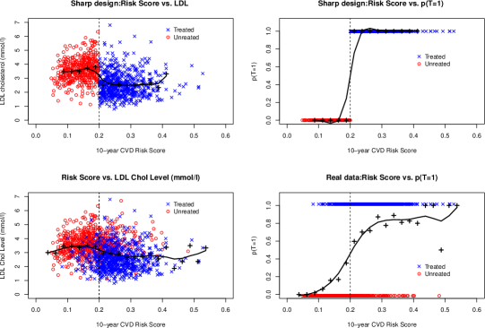
Figure 1: Top row: The sharp design. Bottom row: The real (fuzzy) design. In both cases means within bins and corresponding fitted cubic spline are overlayed.

Figure 2 shows the plots for the binary outcome LDL cholesterol below 2 mmol/L which we analyse in Section 5. While there is no discernible jump in the outcome (left), there is evidence in a jump in the probability of being treated for such patients (right). Taken together, there is sufficient support for a RD design analysis in this context. The corresponding plots for LDL cholesterol dropping below 3 mmol/l are given in the Supplementary Material and show a jumps in the outcome and the probability of treatment.

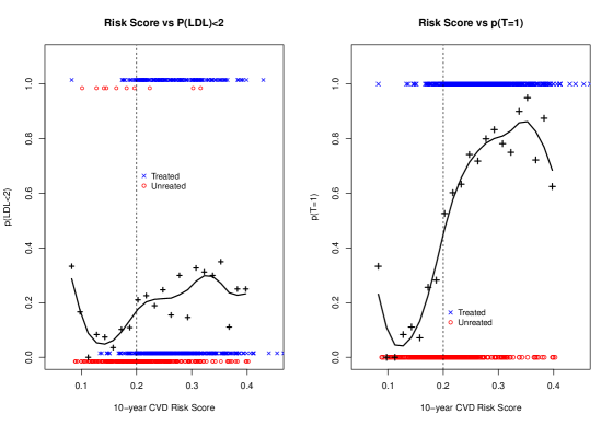
Figure 2: Mean and probability plots for outcome LDL cholesterol going below 2 mmol/l.

2.2 Assumptions and notation

In order for the RD design to be appropriate a number of formal assumptions also have to hold. These assumptions are expressed in different ways (Hahn et al. (2001); Imbens and Lemieux (2008); van der Klaauw (2008); Lee (2008)) and we give a brief overview of them as described in more detail in Geneletti et al. (2015); Constantinou and O’Keeffe (2015). In the binary outcome case we need to make additional assumptions in order to identify the Risk Ratio for the treated our estimator of choice (Didelez et al. (2010); Hernan and Robins (2006)).

We operate within a decision theoretic framework (Dawid (2002)), as this approach makes more explicit the assumptions needed to link causal (experimental) and observational quantities. However the RRT as identified in (2) below and consequently the Bayesian methods we apply do not rely on this framework and can be interpreted within a counterfactual or potential outcomes paradigm.

We express our assumptions in the language of conditional independence following Dawid (1979). We say that if variable $A$ is independent of another $B$ conditional on a third $C$, then $p(A,B\mid C)=p(A\mid C)p(B\mid C)$ and we write $A\mbox{$\perp\!\!\!\perp$}B\mid C$. We refer to our example to anchor the theoretical arguments. Generalising to other contexts is straightforward.

Let $X$ be the 10 year cardiovascular risk score. The threshold indicator $Z$ is such that $Z=1$ if $X\geq 0.2$ and $Z=0$ if $X<0.2$. Let $T$ represent statins prescription (not whether the patient takes the treatment); $T=1$ means statins are prescribed and $T=0$ means they are not. Also, let $\bm{C}=\{\bm{O}\cup\bm{U}\}$ be the set of confounders, where $\bm{O}$ and $\bm{U}$ indicate fully observed and partially or fully unobserved variables, respectively. $Y$ is the binary outcome variable where $Y=1$ if LDL cholesterol is below 2 (resp, 3) and 0 otherwise.

To reflect the fact that these assumptions are only valid around the threshold, we assume throughout the paper an additional conditioning on $X\in[0.2,0.2+h]$ if above the threshold and $X\in[0.2-h,0.2]$ below the threshold for some suitably small $h$. We do not explicitly write this conditioning except where necessary.

Finally, in order to be able to use data around the threshold to estimate quantities with causal meaning we introduce a regime indicator $\Sigma$ as in (Constantinou and O’Keeffe (2015)). $\Sigma$ represents which of the three possible regimes or situations we find ourselves in: the interventional regime (i.e. the RCT), the sharp RD design or the fuzzy RD design.

$$\Sigma=\begin{cases}t,&\mbox{for $T=t$ $(=0,1)$, under the interventional regime;}\\ s,&\mbox{for the sharp RD design;}\\ f,&\mbox{for the fuzzy RD design.}\end{cases}$$

When $\Sigma=t$ we mean that $T$ is set to $t$ with no uncertainty as in an RCT with perfect compliance. In this case it is akin to the “do” operator (Pearl (2001)) or the intervention variable $F$ in Dawid (2002). For clarity we replace conditioning on $\Sigma=\varsigma$ by a subscript on the expectation $E_{\varsigma}(Y\mid X,C)$. It is clear from the definition of $\Sigma$ that both RD designs are types of observational data. By defining $\Sigma$ we can formalise, in terms of conditional independences, when it is possible to make inference about causal quantities from estimates based on observational data. We make two further assumptions involving the regime $\Sigma$:

1. $(C,X,Z)\mbox{$\perp\!\!\!\perp$}\Sigma;$

2. $Y\mbox{$\perp\!\!\!\perp$}\Sigma\mid(C,X,Z,T,)$

Assumption A1 says that the value of the confounders, the assignment variable (and trivially the threshold indicator) are marginally independent of the context in which they arise, i.e. in an experiment or within and RD design. Under A2, the value of the outcome does not depend on the regime if we take into account the confounders, the assignment variable (and trivially the threshold indicator) as well as the prescription status. These assumptions are termed “sufficiency” assumptions (Dawid and Didelez (2010)) and allow us to move from the interventional to the RD design regimes.

2.3 RD design assumptions

The first three RD design assumptions are essentially IV assumptions whilst the fourth is specific to the RD design. See Geneletti et al. (2015) for more details and interpretation.

1. Association of treatment with threshold indicator: $Z\not\!\!\!\,\mbox{$\perp\!\!\!\perp$}T\mid\Sigma$

2. Independence of guidelines:$Z\mbox{$\perp\!\!\!\perp$}\bm{C}\mid(X,\Sigma)$,
   A weaker version (i.e. within strata of $\bm{O}$) is: $Z\mbox{$\perp\!\!\!\perp$}\bm{U}\mid(X,\bm{O},\Sigma)$.

3. Unconfoundedness: $Y\mbox{$\perp\!\!\!\perp$}Z\mid(T,\bm{C},X,\Sigma)$.

4. Continuity: The expectation of the outcome $E_{\varsigma}(Y\mid X,C,Z,T=t)$ is continuous at $X=x_{0}$ for $t\in\{0,1\}$ and $\varsigma=\{s,f\}$.

2.4 MSMM estimator and associated assumptions

We estimate risk ratios in our analysis as these are of primary interest and most suited to our method of analysis. In the epidemiological literature odds ratios are usually estimated as they are easily obtained from logistic regressions. However simple estimators of causal odds ratios are typically more biased than risk ratio estimators (Didelez et al. (2010)).

We focus on estimating the Risk Ratio for the Treated (RRT) defined as follows:

$$\frac{E\{E_{1}(Y\mid Z)\mid T=1\}}{E\{E_{0}(Y\mid Z)\mid T=1\}}$$ (1)

which is the binary equivalent of the effect of treatment on the treated. This quantity can be identified in a fuzzy design provided additional assumptions, listed below, are satisfied. The RRT can be interpreted as ratio of the risk for those who were treated relative to those who were eligible for treatment. In our example we can think about this as follows: statins treatment is made available to GP-patient pairs (GPPs) around the threshold thus all these GPPs are eligible for statin prescription. However, of these only some take up the treatment. The RRT is a comparison of the outcomes for the patients from GPPs who prescribed statins relative to all the patients who were eligible and is the binary version of the effect of treatment on the treated(Geneletti and Dawid (2010)).

The RRT in (1) can be identified from observational RD design data when $Y$, $Z$ and $T$ are binary if in addition to R1-R4 the following assumptions hold (Didelez et al. (2010)).

1. Log-linear in t
   $\mbox{log}[E_{1}(Y\mid T=t,Z=z)]-\mbox{log}[E_{0}(Y\mid T=t,Z=z)]$ is linear in the treatment.

2. No T-Z interaction on the multiplicative scale
   This assumption is known as the no-effect modification assumption (NEM).

When Assumptions R1-R4 and M1-M2 hold, $\Sigma$ is defined as in Section 2.2 and conditional independences A1 and A2 hold, we can use estimators that have been derived in the binary instrumental variables literature in the context of the RD design without further deriving any results. Thus we obtain the following formula for the RRT (Hernan and Robins (2006); Clarke and Windmeijer (2010)):

$$\mbox{RRT}_{\varsigma}=1-\displaystyle\frac{E_{\varsigma}(Y\mid Z=1)-E_{\varsigma}(Y\mid Z=0)}{E_{\varsigma}(Y\bar{T}\mid Z=1)-E_{\varsigma}(Y\bar{T}\mid Z=0)},$$ (2)

where $\bar{T}=(1-T)$ and $\varsigma=\{s,f\}$. Equivalent expressions and details of their derivation and interpretation can be found in Didelez et al. (2010); Abadie (2003); Angrist (2001). Note that when $\Sigma=s$, (2) reduces to the causal risk ratio. As fuzzy designs are the norm and sharp the exception we drop the subscript _ς for notational clarity, so that implicitly $\Sigma=t$.

For the RRT to be above 1, either the numerator or the denominator must be negative – but not both. In our context we would expect to see a positive numerator as we would expect there to be more individuals with low cholesterol levels above than below the threshold. This is because the threshold and the treatment are positively correlated and treatment reduces cholesterol. The denominator involves the product of $Y$ and ‘no treatment’ $\bar{T}=(1-T)$. As we expect statin treatment to lower cholesterol and be associated with the threshold indicator, we expect the denominator to be negative. This is reflected in the results in Section 5, where the RRT is above 1 for both outcomes and most bandwidths except the smallest for the outcome LDL below 2.

Assumption M2 requires that whether the LDL cholesterol level is below 2 (resp. 3) does not depend on an interaction term between $T$ (statin prescription) and $Z$ (whether the risk score exceeds 20% on the log scale). If there were an interaction term it would mean that the GPs above and below the threshold would be different with respect to their ability to predict the outcome. This is unlikely to be the case.

The RRT as show in Equation (2) also identifies the local causal risk ratio, the binary equivalent of the complier average causal effect (Frangakis and Rubin (2002); Imbens and Angrist (1994)).

3 Models

The models in Sections 3.2 and 3.3 are embedded in a Bayesian framework. We first obtain a full posterior MCMC sample for each of the relevant parameters in the models described in Section 3.2 and combine these to induce a posterior sample for the RRT. When we add prior constraints in Section 3.3 we sample the RRT directly. From the posterior samples we easily obtain variances and interval estimates without having to rely on bootstrap methods or asymptotic arguments, as is the case with the frequentist estimators.

We present a number of possible models to estimate the components. We mostly use the same types of models in the numerator and the same type in the denominator. However, we do mix different models in the numerator and denominator where we consider this necessary. Generally speaking we write the estimates for the RRT as follows: $\mbox{RRT}_{num.denom}$ where num indicates the form of the numerator and denom the denominator in the fraction in (2).

3.1 Interaction vs Product models

The denominator of the fraction in the expression for the RRT (henceforth only “the denominator”) is given by $E(Y\bar{T}\mid Z=1)-E(Y\bar{T}\mid Z=0)$. We can break up the individual terms further as follows:

$$E(Y\bar{T}\mid Z=z)=E(Y\mid\bar{T},Z)E(\bar{T}\mid Z).$$ (3)

In our analysis, we produce estimates for both of these models. We call interaction models those which use the formulation on the left hand side of equation (3) and product models those that use the formulation on the right hand side. Our motivation for including analyses with the product of two conditional probabilities as in (3) is that the data for the product term are sparse (see Supplementary materials). By using $Y$ alone this is mitigated. We also consider zero inflated Poisson regression models (Lambert (1992)) to address this but results are not substantially different.

3.2 Poisson regression models

The first set of models we considered estimates all the components in the RRT using Poisson regression models, in line with assumption M1. It is easy to verify that if the same parametric form can be assumed to hold for experimental and observational regimes then a log-linear relationship in $t$ follows for each of the components of (2).

Let $X^{*}=X-0.2$, we fit Poisson regressions in both the numerator and the denominator:

$$\mbox{Numerator}:= \begin{cases}y_{i_{z}}\sim\mbox{Poisson}(\mu_{i_{z}})\\ \mbox{log}(\mu_{i_{z}})=\alpha_{z}+\beta_{z}x_{i_{z}}^{*}\end{cases}\mbox{Denominator}:= \begin{cases}y\bar{t}_{i_{z}}\sim\mbox{Poisson}(\nu_{i_{z}})\\ \mbox{log}(\nu_{i_{z}})=\delta_{z}+\gamma_{z}x_{i_{z}}^{*}\end{cases}$$

with priors $\alpha_{z},\beta_{z},\delta_{z},\gamma_{z}\stackrel{{\scriptstyle iid}}{{\sim}}\mbox{Normal}(0,100)$, $i_{z}=1,\ldots,n_{z}$ and $z\in\{0,1\}$ throughout.

We put relatively vague priors on the regression coefficients. Tighter priors such as those suggested in Gelman et al. (2008) have been considered, but results are not very sensitive to the choice of prior. As we centre the risk score at the threshold, the parameter of interest in all the regressions is the exponential of the intercept term. The posterior MCMC samples of the parameters $\alpha_{1}$, $\alpha_{0}$, $\delta_{1}$ and $\delta_{0}$ can be used to characterize $E(Y\mid Z=1)$, $E(Y\mid Z=0)$, $E(Y\bar{T}\mid Z=1)$, and $E(Y\bar{T}\mid Z=0)$ respectively and then combined to obtain the posterior sample for the RRT. The model described above has the interaction model denominator:

$$\mbox{RRT}_{pois.pois} =1-\frac{\Pi_{pois}}{\Psi_{pois}}\qquad\mbox{where}$$

$$\Pi_{pois}=\mbox{exp}(\alpha_{1})-\mbox{exp}(\alpha_{0})\qquad \mbox{and }\qquad\Psi_{pois}=\mbox{exp}(\delta_{1})-\mbox{exp}(\delta_{0})$$

We also consider an interaction model where the denominator is based on a flexible Binomial model as used in Geneletti et al. (2015). In this model the prior information is used to create distance between the two elements in the denominator of the fraction in the RRT in (2). This often stabilises the results because it pushes the difference in the probability of treatment at the threshold away from zero and thus inflates the fraction in (2). In this case the denominator is defined as

Denominator: $$y\bar{t}_{i_{z}}\sim\mbox{Binomial}(q_{z},n_{z})$$

$$\mbox{priors:}\,\mbox{logit}(q_{1}) \sim\mbox{Normal}(-3,1)\qquad\mbox{and}\qquad\mbox{logit}(q_{0})\sim\mbox{Normal}(3,1)\qquad\mbox{so}\,\,\Psi_{flex}=q_{1}-q_{0}.$$

This results in the interaction model

$$\mbox{RRT}_{pois.flex}=1-\frac{\Pi_{pois}}{\Psi_{flex}}.$$

We now consider the product denominator as follows:

$$\mbox{Denominator.prod}= \begin{cases}y_{i_{z}}\sim\mbox{Poisson}(\theta_{iz})\\ \mbox{log}(\theta_{i_{z}})=\delta_{z}+\gamma_{z}x_{i_{z}}+\kappa_{z}\bar{t}_{i_{z}}\\ t_{i_{z}}\sim\mbox{Binomial}(r_{z},n_{z})\end{cases}$$

priors: $$\mbox{logit}(r_{1})\sim\mbox{Normal}(-3,1)\qquad\mbox{and }\qquad\mbox{logit}(r_{0})\sim\mbox{Normal}(3,1).$$

We then combine the conditional probabilities as follows

$$E(Y\bar{T}\mid Z=z)=(\delta_{z}+\kappa_{z})\times r_{z},$$

as we are interested in the case where both $Y$ and $\bar{T}$ are equal to 1. Note that we use the Binomial flex model again for the probability of $\bar{T}$ as this was less variable than regression-based models, in this case. Thus we obtain $\mbox{RRT}_{pois.prod.flex}$ as follows:

$$\mbox{RRT}_{pois.prod.flex}=1-\frac{\Pi_{pois}}{\Psi_{prod.flex}}$$

where $\Psi_{prod.flex}=\mbox{exp}(\delta_{1}+\kappa_{1})r_{1}-\mbox{exp}(\delta_{0}+\kappa_{0})r_{0}$.

3.3 Constraints

The RRT can drop below zero if the fraction in (2) exceeds one (Clarke and Windmeijer (2010)). We avoid the problem by imposing a priori constraints on the distribution of the RRT which force the RRT to remain within the acceptable bounds.

Imposing prior constraints is easy in the Bayesian framework. We put a Gamma prior on the RRT with most of the mass close to 1, as we do not want to encourage a large risk ratio. The most straightforward constraint was to make $\alpha_{1}$ a function of the other variables above the threshold so that we could place a prior on the RRT. We could equally have chosen $\alpha_{0}$. We write out the changes the model implies to the priors below:

$$\mbox{RRT}_{pois.pois}\sim\mbox{Gamma}(3,1)\qquad\mbox{and}\qquad\alpha_{1}=\mbox{log}\{(1-\mbox{RRT}_{pois.pois})\Psi_{pois}+\mbox{exp}(\alpha_{0})\}$$

where $\exp(\alpha_{1})-\exp(\alpha_{0})=\Pi_{pois}$ and there is of course no prior on $\alpha_{1}$. Similar changes can be made to all the RRTs with any of the other models presented in Section 3. It is also possible to impose constraints on logistic regression based estimates.

3.4 Generalized Method of Moments analysis

In order to assess the performance of our Bayesian estimators, we compared them to some of the most common estimators for binary outcomes in the IV literature. These include the Generalized Method of Moments (GMM) MSMM estimator (Clarke et al. (2015)), the Wald Risk Ratio (Didelez et al. (2010)) and a final method based on a single estimating equation (Burgess et al. (2014)). We give a brief overview and show results in Table 1 of Section 5 for the first of these methods as it outpeformed the other two. Details and results for the other methods can be found in the Supplementary material.

Clarke et al. (2015) showed that the semi-parametric MSMM estimator in equation (2) can be estimated efficiently by the Generalized Method of Moments (GMM). The moment conditions

$$E\left[\begin{gathered}Y\exp(-\beta_{0}X)-\alpha_{0}\\ \{Y\exp(-\beta_{0}X)-\alpha_{0}\}Z\end{gathered}\right]=\left(\begin{gathered}0\\ 0\end{gathered}\right)$$

lead to the estimation of $\alpha_{0}$ and $\beta_{0}$ by the method of moments.

4 Simulation study

We set up a simple simulation study aimed at examining the properties of the models presented in Section 3 under two levels of unobserved confounding ($U$), two levels of IV strength ($Z$) and three causal effects. Thus we performed simulations for 12 Scenarios. We based our simulated data set on the larger data set from which the one described in Section 2 and analysed in Section 5 was obtained. Thus we used the original values for the risk score $X$ and the standardized HDL cholesterol level as unobserved confounder $U$. The threshold indicator $Z$ was defined deterministically as $Z_{i}=0$ if $X_{i}<0.2$ and $Z_{i}=1$ otherwise. For each simulation and in the real data in Section 5 we run the analyses in each of four bandwidths identified by values $h=\{0.025,0.05,0.075,0.1\}$ and assess the sensitivity of the results to these changes.

We generate assigned treatment and outcome in order to get different settings of strength of instrument (Weak or Strong), unobserved confounding (Low or High) and three different risk ratios: 1, 2.11 and 4.48 corresponding to no, low and high causal effect. More details about the simulation mechanism are in the Supplementary material.

We produced exploratory plots like those introduced in Section 2 for all the simulated scenarios. Briefly, for high causal effects all scenarios showed a clear jump at the threshold although it was smaller in the weak IV high confounding scenario. For the low causal effects results were variable. No jump was discernible in the weak IV high confounding scenario but a clear jump was visible in the strong IV scenarios. Finally for the no-effect scenarios no jump was visible as expected. A selection of plots can be seen in the Supplementary Materials.

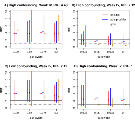
Figure 3: Comparison of the results in 4 out of 12 simulated scenarios.

We obtained results for Bayesian constrained and unconstrained models as well as a number of frequentist estimates and the Balke-Pearl bounds which are available on website xxx In the body of the paper we only present results for the constrained models as in many scenarios (in particular for small bandwidths, high confounding and weak instruments) the posterior MCMC sample for the unconstrained models contained values below zero. In addition, while convergence was reached for the relevant parameters, there were some extreme results due to small values in the denominator that occasionally led to inflated mean estimates. Medians for the unconstrained models and means for the constrained models were generally close although the constrained model estimates were typically smaller. We thought this might be due to the Gamma prior pulling the RRT in the constrained models towards one. However upon investigation we saw that results were not sensitive to the choice of prior.

Figure 3 shows the results for 3 estimators in 4 out of 12 simulated scenarios (full results for all simulated scenarios are available on request). We selected pois.flex (in red) and pois.prod.flex (blue). Also we plot the MSMM estimator obtained using GMM (orange). For each estimator, a solid coloured line represents the 95% confidence or credible interval while the dot represents the mean value. The true risk ratio is shown using a solid horizontal black line, and in case the true effect differs from 1, a dotted line indicates the absence of effect.

In panel A the risk ratio is 4.48. Here the Bayesian model outperforms the others. The mean RRT is closer to the true value and the intervals are considerably narrower, especially when small bandwidths are considered.

In panels B and C the true risk ratio is equal to $2.11$ and the estimators show mixed behaviour. Results in B are relative to the worst possible scenario, where confounding is high and the instrument is weak. All estimators underestimate the real effect and all 95% intervals include 1. Bayesian Point estimates are less biased and their intervals always include the true value. This is not the case for GMM whose intervals do not include 2.11 for most bandwidths.

Results in C are for the low confounding-weak instrument scenario. Bayesian estimators show similar behaviour for all values of $h$, overestimating the true value, but including it within the 95% interval. The GMM based method gives wider and misleading intervals which include the value 1 in the smaller bandwidths $h\in\{0.025,0.05\}$.

Finally panel D represents the scenario with high level of confounding, weak instrument and no effect. With $h>0.025$ the GMM estimator perform better in terms of both point and interval estimation however it is very sensitive to the sample size. In $h=0.025$ the intervals are very wide. The Bayesian estimates result in very high point estimates but their intervals include 1.

Overall the Bayesian estimators appear to be more robust to IV strength, confounding levels and size of causal effect. For small bandwidths none of the methods performs particularly well when the risk ratio is small or one, however the Bayesian estimator compares favourably with the competing methods in the borderline cases. A possible reason for the robustness of Bayesian estimators in the extreme scenarios is that continuous information is used in estimating the components of the RDD whereas the GMM (and other frequentist) estimates are based on binary data only.

5 Example: Statin prescription

5.1 Data

The data we consider are a subset of The Health Improvement Network (THIN) data set. THIN are primary care data for over 500 practices in the UK and include a large number of individual patient, diagnostic and prescription information. We focus on a subset of 1386 male patients between 50 and 70 who did not smoke or have diabetes in the year 2008. We investigate whether statin prescription lowers the LDL cholesterol to below two and three mmol/L, recommended levels for high and low risk individuals respectively.

From trials (Ward et al. (2007)) we know that statins are effective in lowering cholesterol. As LDL cholesterol tends to decrease quickly within a month of uptake and our data span the 6 months around the cholesterol measurement we can use our binary outcomes RD design to determine whether statins result in people achieving LDL cholesterol targets within a small time window. Our approach is also useful when we are interested in whether a drug acts on a relevant marker of a disease which is easier to measure and is affected quickly by treatment.

5.2 Preliminary analyses

Prior to estimating the RRT we investigated whether a Poisson regression was an appropriate models for the data. Model fit was good overall and there was no evidence for overdispersion.

In line with recent recommendations regarding what should be presented in IV analyses (Swanson and Hernan (2013)) we performed F-tests to determine IV weakness for non-linear situations (Windmeijer and Didelez (2016)) for both binary outcomes (LDL below 2 and below 3). The F-values ranged from 10 (for bandwidth 0.025) to 211 (for bandwidth 0.1) with p-values significant at the 5% level throughout. The Balke-Pearl bounds Balke and Pearl (1997); Palmer et al. (2011) were also in line with our results.

5.3 Main analysis

	All, LDL$<3$			All, LDL$<2$
	Mean	L95	U95	Mean	L95	U95
$h=0.025$
pois.flex	3.12	1.32	5.62	2.59	0.86	5.57
pois.pois	3.98	1.32	8.16	2.96	0.89	6.42
pois.prod.flex	3.89	1.11	6.16	2.77	0.77	5.81
GMM	3.99	1.30	12.21	8.39	1.49	47.37
$h=0.05$
pois.flex	3.95	1.51	7.39	2.59	0.99	4.91
pois.pois	4.01	1.12	7.93	2.81	0.85	5.92
pois.prod.flex	4.17	1.08	8.14	2.64	0.85	5.34
GMM	4.53	2.29	8.93	4.49	3.04	29.62
$h=0.075$
pois.flex	3.76	1.48	7.84	2.63	1.02	4.76
pois.pois	4.33	1.47	8.60	3.19	0.95	6.13
pois.prod.flex	4.60	1.57	8.60	2.80	1.01	5.33
GMM	4.22	2.55	7.03	6.68	3.07	14.56
$h=0.1$
pois.flex	3.69	1.42	6.82	4.20	1.02	7.13
pois.pois	4.02	1.37	7.60	6.82	1.25	4.50
pois.prod.flex	3.99	1.36	7.36	2.70	1.31	4.86
GMM	3.76	2.60	5.44	7.36	3.73	14.55

Table 1: The table contains the results for estimates of the constrained RRT as well as the GMM based estimator.

We fitted our models using JAGS (Plummer (2003)) with two chains, a burn-in of 10,000 iterations and a further 50,000 iterations. Our posterior samples were based on the last 1000 iterations. On average each estimator took 5 minutes to run on a standard PC. Convergence was reached for all relevant parameters.

Overall the results indicate a positive effect of statin treatment on LDL cholesterol levels for patients in our sample with a large (if not universally significant) two to three-fold increase in the probability of achieving the target LDL cholesterol level within 6 months of prescription for those prescribed relative to those eligible. This is especially true for the target of reducing the LDL cholesterol level to below 3 mmol/L.

Table (1) shows for each bandwidth the mean, upper and lower 95% interval estimates for the RRT with constrained models and the GMM. The plots in Figure 4 show the RRT estimates for the unconstrained models in the left and the constrained models in the right for LDL below 3. We can see that in particular for the low bandwidths where the data are sparse the estimates using the unconstrained models are very variable. Similar plots displaying a similar pattern for the LDL below 2 are given in the Supplementary Materials. Overall the constrained estimates both reduce the variability of the estimates and ensure that they remain above zero.

Generally, Bayesian estimates are similar and increase slightly as the bandwidth increases. The estimates for LDL$<$3 mmol/L are slightly larger than those for LDL$<2$ and always significant. If you consider that the median LDL cholesterol for the untreated is approximately 4 then it is easy to see that to reduce the level to below 2 when statins are thought to reduce cholesterol by up to 2mmol/L is going to be difficult. Thus it makes sense that for LDL$<$2 mmol/L the RRT is not significant for small bandwidths.

When we compare the results of the GMM methods to ours we see that for the LDL below 3 scenarios are broadly similar. For the outcome LDL below 2 however results are different. For all the bandwidths the means of the GMM are very high and the intervals are wide. Also, from our simulation studies – which are based on the same data – we know that for small bandwidths (i.e. small sample sizes) the GMM estimators over-estimate the effects and are less robust in general than the Bayesian estimates.

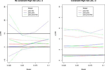
Figure 4: On the left and right are the means and 95% credible intervals when the models are unconstrained and constrained respectively. The y-axis have different scales.

6 Conclusions

In this paper we use the RD design to develop a Bayesian method to estimate the risk ratio for the treated (Hernan and Robins (2006); Clarke and Windmeijer (2010)) which does not stray below zero. We do this by imposing prior constraints. As this represents a very strong assumption, we assessed how much results were affected. Counter to our expectation results from our simulations and applied example constraining the models to be above zero did not result in higher RRT estimates, nor were results very sensitive to prior specification. Specifically varying the values of the Gamma distribution on the RRT (e.g., by moving the mass further from 1) or even using a different prior with positive support (i.e., the log-normal) did not alter results substantially. Instead the constrained models stabilised the posterior MCMC sample.

The fact that the RTT as identified by (2) has no built-in safe guard to dropping below zero raises some questions as to its appropriateness as a risk ratio estimator. It is not easy to identify causal quantities when all elements are binary and as a consequence a number of strong assumptions must be met. It is likely that some will hold only approximately. If we suspect that assumptions R1-R4 do not hold then there is no point in attempting an RD analysis or estimating the RRT from these data; however if we think of M1-M2 as holding only approximately around the threshold then we can view this as a model misspecification problem and the RRT as an approximation to the true underlying effect.

Our results compared favourably to those of the generalised method of moments as well and other frequenstist estimators. In particular they were more robust to weak instruments, high levels of confounding and low effects in the simulation studies. They also produced more credible results in our application.

A further advantage of our approach is that as we model the individual components of the RRT jointly (possibly subject to constraints) we can be very flexible in our choice of models. We propose Poisson regression based models on theoretical grounds and because in the RD design we can exploit the continuous information in the risk score. However Poisson regressions do not guarantee that the coefficients or predictions of the regression behave like probabilities. While our results do not misbehave in this way it is something to bear in mind. Due to the flexible approach we have developled we also have implemented models identical to those we propose where logs are replaced by logits and exponentials with expits. Futher we have tried zero-inflated Poisson regression models and Binomial models. Results are broadly similar especially for the regression based models. JAGS code for some of these models is given in the Supplementary materials and results are available on request. It is also feasible to use splines or other semi-parametric models.

There are also a number of papers that focus on estimating causal odds ratios, notably Vansteelandt et al. (2011); Vansteelandt and Goetghebeur (2003); van der Laan et al. (2007). While we have not done this here it should be possible to use the double logistic causal odds ratio estimator in a way similar to how we use the MSMM risk ratio estimator although additional requirements (e.g. specifying a model for $P(Y\mid T,Z)$) need to be taken into account.

References

- Abadie [2003] A Abadie. Semiparametric instrumental variable estimation of treatment response models. Journal of Econometrics, 113(2):231–263, APR 2003. ISSN 0304-4076. doi: –10.1016/S0304-4076(02)00201-4˝.
- Angrist [2001] JD Angrist. Estimation of limited dependent variable models with dummy endogenous regressors: Simple strategies for empirical practice. Journal of Business & Economic Statistics, 19(1):2–16, JAN 2001. ISSN 0735-0015. doi: –10.1198/07350010152472571˝.
- Balke and Pearl [1997] A. Balke and J. Pearl. Bounds on treatment effects from studies with imperfect compliance. Journal of the American Statistical Association, 92(439):1171–1176, 1997.
- Bor et al. [2014] J. Bor, E. Moscoe, P. Mutevedzi, M. L. Newell, and T. Barnighausen. Regression discontinuity designs in epidemiology: causal inference without randomized trials. Epidemiology, 25(5):729–737, 2014. doi: 10.1097/EDE.0000000000000138.
- Burgess et al. [2014] S. Burgess, R. Granell, T. M. Palmer, J. A. C. Sterne, and V. Didelez. Lack of identification in semiparametric instrumental variable models with binary outcomes. Am. J. Epidemiol., 2014. doi: 10.1093/aje/kwu107.
- Calonico et al. [2015] S. Calonico, M. D. Cattaneo, and R. Titiunik. Robust nonparametric confidence intervals for regression discontinuity designs. Econometrica, 82(6):2295 – 2326, 2015.
- Clarke et al. [2015] P. S. Clarke, T. M. Palmer, and F. Windmeijer. Estimating structural mean models with multiple instrumental variables using the generalised method of moments. Statistical Science, 30(1):96–117, 2015. doi: 10.1214/14-STS503.
- Clarke and Windmeijer [2010] Paul S. Clarke and Frank Windmeijer. Identification of causal effects on binary outcomes using structural mean models. BIOSTATISTICS, 11(4):756–770, OCT 2010. ISSN 1465-4644. doi: –10.1093/biostatistics/kxq024˝.
- Clarke and Windmeijer [2012] P.S. Clarke and F. Windmeijer. Instrumental variable estimators for binary outcomes. Journal of the American Statistical Association, 107(500):1638–1652, 2012. doi: 10.1080/01621459.2012.734171.
- Constantinou and O’Keeffe [2015] P. Constantinou and A. G. O’Keeffe. Regression discontinuity design: A decision thoretic approach. submitted to …, 2015.
- Dawid [1979] A P. Dawid. Conditional independence in statistical theory. Journal of the Royal Statistical Society, Series B (Statistical Methodology), 41(1):1–31, 1979.
- Dawid [2002] AP Dawid. Influence diagrams for causal modelling and inference. Iternational Statistical Review, 70(2):161–189, AUG 2002. ISSN 0306-7734.
- Dawid and Didelez [2010] A.P. Dawid and V. Didelez. dentifying the consequences of dynamic treatment strategies: A decision-theoretic overview. Statistics Surveys, 4:184–231, 2010.
- Didelez et al. [2010] V. Didelez, S. Meng, and N. A. Sheehan. Assumptions of iv methods for observational epidemiology. Statistical Science, 25(1):22–40, 2010. doi: 10.1214/09-STS316.
- Frangakis and Rubin [2002] Constantine E. Frangakis and Donald B. Rubin. Principal stratification in causal inference. Biometrics, 58(1):21–29, 2002. ISSN 1541-0420. doi: 10.1111/j.0006-341X.2002.00021.x. URL http://dx.doi.org/10.1111/j.0006-341X.2002.00021.x.
- Gelman et al. [2008] A. Gelman, Jakulin A., M. Pittau, and Y Su. A weakly informative default prior distribution for logistic and other regression models. The Annals of Applied Statistics, 2(4):1360–1383, 2008.
- Geneletti and Dawid [2010] S. Geneletti and A.P. Dawid. The effect of treatment on the treated: a decision theoretic perspective. In M. Ilari, F. Russo, and J. Williamson, editors, Causality in the Sciences. Oxford University Press, 2010.
- Geneletti et al. [2015] S. Geneletti, A. G. O’Keeffe, L. D. Sharples, S. Richardson, and G. Baio. Bayesian regression discontinuity designs: incorporating clinical knowledge in the causal analysis of primary care data. Statistics in Medicine, 2015. doi: 10.1136/bmj.g5293.
- Hahn et al. [2001] JY Hahn, P Todd, and W Van der Klaauw. Identification and estimation of treatment effects with a regression-discontinuity design. Econometrica, 69(1):201–209, Jan 2001. ISSN 0012-9682. doi: 10.1111/1468-0262.00183.
- Hernan and Robins [2006] MA Hernan and JM Robins. Instruments for causal inference - An epidemiologist’s dream? Epidemiology, 17(4):360–372, Jul 2006. ISSN 1044-3983. doi: 10.1097/01.ede.0000222409.00878.37.
- Imbens and Kalyanaraman [2012] G. Imbens and K. Kalyanaraman. Optimal bandwidth choice for the regression discontinuity estimator. Review of Economic Studies, 2012.
- Imbens and Angrist [1994] G W. Imbens and J D. Angrist. Identification and estimation of local average treatment effects. Econometrica, 62(2):467–475, 1994.
- Imbens and Lemieux [2008] Guido W. Imbens and Thomas Lemieux. Regression discontinuity designs: A guide to practice. Journal of Econometrics, 142(2):615 – 635, 2008. ISSN 0304-4076. doi: 10.1016/j.jeconom.2007.05.001. The regression discontinuity design: Theory and applications.
- Lambert [1992] D. Lambert. Zero-inflated Poisson regression, with an application to defects in manufacturing. Technometrics, 34(1):1–14, FEB 1992. ISSN 0040-1706. doi: –10.2307/1269547˝.
- Lee [2008] David S. Lee. Randomized experiments from non-random selection in US House elections. Journal Of Econometrics, 142(2):675–697, FEB 2008. ISSN 0304-4076. doi: 10.1016/j.jeconom.2007.05.004. Conference on the Regression Discontinuity Design, Banff, CANADA, MAY 00, 2003-SEP 08, 2005.
- Palmer et al. [2011] T. M. Palmer, R. R. Ramsahai, V. Didelez, and N. A. Sheehan. Nonparametric bounds for the causal effect in a binary instrumental-variable model. The Stata Journal, 11(3):345–367, 2011.
- Pearl [2001] Judea Pearl. Causality. Cambridge University Press, 2001.
- Plummer [2003] M. Plummer. Jags: A program for analysis of bayesian graphical models using gibbs sampling. 2003.
- Swanson and Hernan [2013] S.A. Swanson and Miguel A. Hernan. Commentary: How to report instrumental variable analyses (suggestions welcome). Epidemiology, 24(3):1044–3983, 2013.
- Thistlethwaite and Campbell [1960] DL. Thistlethwaite and DT. Campbell. Regression-Discontinuity Analysis - An alternative to the ex-post-facto experiment. Journal of Educational Psychology, 51(6):309–317, 1960.
- van der Klaauw [2008] G. van der Klaauw. Regression-discontinuity analysis: A survey of recent developments in economics. Labour, 22(2):219–245, 2008.
- van der Laan et al. [2007] Mark J. van der Laan, Alan Hubbard, and Nicholas P. Jewell. Estimation of treatment effects in randomized trials with non-compliance and a dichotomous outcome. Journal of the Royal Statistical Sociery Series B-Statistical Methodology, 69(3):463–482, 2007. ISSN 1369-7412. doi: –10.1111/j.1467-9868.2007.00598.x˝.
- Vansteelandt and Goetghebeur [2003] S Vansteelandt and E Goetghebeur. Causal inference with generalized structural mean models. Journal of the Royal Statistical Society Series B-Statistical Methodology, 65(4):817–835, 2003. ISSN 1369-7412. doi: –10.1046/j.1369-7412.2003.00417.x˝.
- Vansteelandt et al. [2011] Stijn Vansteelandt, Jack Bowden, Manoochehr Babanezhad, and Els Goetghebeur. On instrumental variables estimation of causal odds ratios. Statist. Sci., 26(3):403–422, 08 2011. doi: 10.1214/11-STS360. URL http://dx.doi.org/10.1214/11-STS360.
- Ward et al. [2007] S. Ward, L. Jones, A. Pandor, M. Holmes, R. Ara, A. Ryan, W. Yeo, and N. Payne. A systematic review and economic evaluation of statins for the prevention of coronary events. Health Technology Assessment, 11(14), 2007.
- Windmeijer and Didelez [2016] F. Windmeijer and V. Didelez. Methods for binary outcomes. In G Davey-Smith, editor, Mendelian Randomization: How genes can reveal the biological and environmental causes of disease, To appear. Oxford University Press, 2016.