The Kinematic Image of RR, PR, and RP Dyads

Summary

We provide necessary and sufficient conditions for admissible transformations in the projectivised dual quaternion model of rigid body displacements and we characterise constraint varieties of dyads with revolute and prismatic joints in this model. Projective transformations induced by coordinate changes in moving and/or fixed frame fix the quadrics of a pencil and preserve the two families of rulings of an exceptional three-dimensional quadric. The constraint variety of a dyad with two revolute joints is a regular ruled quadric in a three-space that contains a “null quadrilateral”. If a revolute joint is replaced by a prismatic joint, this quadrilateral collapses into a pair of conjugate complex null lines and a real line but these properties are not sufficient to characterise such dyads. We provide a complete characterisation by introducing a new invariant, the “fiber projectivity”, and we present examples that demonstrate its potential to explain hitherto not sufficiently well understood phenomena.

KEYWORDS: Kinematic map, dual quaternion, Study quadric, null cone, revolute joint, prismatic joint, fiber projectivity, vertical Darboux motion.

1 Introduction

A common technique in theoretical and applied kinematics is the use of a point model for the group $\mathrm{SE}(3)$ of rigid body displacements. One prominent example is the projectivised dual quaternion model of $\mathrm{SE}(3)$ which exhibits particularly nice geometric and algebraic properties ^{1; 2; 3; 4}. In this article, we revisit some fundamental concepts related to this model, the transformation group generated by coordinate changes in the moving and the fixed frame and the kinematic images of dyads with revolute and prismatic joints. While numerous necessary conditions on these objects are well-known, we contribute sets of provably sufficient conditions.

Our characterisation of the transformation group generated by coordinate changes in fixed and moving frame (Section 3) is based on the pencil of quadrics spanned by the Study quadric and null cone. These are quadrics corresponding to dual quaternions of real norm and purely dual norm, respectively. Admissible transformations fix each member of this pencil and, in addition, preserve the two families of rulings on a further quadric in a subspace of dimension three. This leads to the important distinction between “left” and “right” rulings. At this point we also introduce a further invariant, the “fiber projectivity”, which will be crucial in our latter characterisation of dyads with prismatic joints in Section 5.

The relative position of two rigid bodies can be constrained by a link or a sequence of links. Fixing one of the two bodies, the collection of all possible poses (position and orientation) of the other is called a constrained variety. These are important objects in the study of open and closed kinematic chains, in linkage synthesis or analysis and other fields. In Section 4, we characterise constraint varieties generated by dyads of two revolute joints (“RR dyads”) as regular ruled quadrics in the Study quadric that contain four complex rulings of the null cone.

In Section 5 we extend this result to dyads containing one prismatic and one revolute joint (“RP dyads” and “PR dyads”). It is tempting to view them as limiting cases of RR dyads where one joint axis becomes “infinite” (lies in the plane at infinity). Indeed, their kinematic image is a regular ruled quadric in the Study quadric that intersects the null cone in two complex lines and a real transversal line. Nonetheless, this viewpoint is not complete because of the possibility of commuting R and P joints (“cylindrical joints”). A closer investigation leads us to a more refined concept involving the fiber projectivity which allows to distinguish between the RP, the PR, and the cylindrical case.

We conclude this paper with an application of our results to a recently presented non-injective extension of the classical kinematic map ⁵. Here, commuting RP dyads appear naturally as kinematic images of straight lines. We use this to prove that the extended kinematic image of a straight line is, in general, a vertical Darboux motion.

Some parts of this paper, mostly Section 4 and the computations in the appendix, overlap with a previously published conference paper ⁶. The investigation on the group of admissible transformation in Section 3, the characterisation of RP and PR dyads in Section 5, and the relation of straight lines in extended kinematic image space to vertical Darboux motions in Section 6 are new.

2 Preliminaries

This article’s scene is the projectivised dual quaternion model of spatial kinematics. Here, we give a very brief introduction to this model for the purpose of settling our notation. More details will be introduced in the text as needed. For more thorough introductions to dual quaternions and there relations to kinematics we refer to Section 3 in Klawitter (2015) ⁴ or Section 11 of Selig (2005) ².

The dual quaternions, denoted by $\mathbb{D}\mathbb{H}$, form an associative algebra in $\mathbb{R}^{8}$ where multiplication of the basis elements $1$, $\mathbf{i}$, $\mathbf{j}$, $\mathbf{k}$, $\varepsilon$, $\varepsilon\mathbf{i}$, $\varepsilon\mathbf{j}$, and $\varepsilon\mathbf{k}$ is defined by the rules

$$\mathbf{i}^{2}=\mathbf{j}^{2}=\mathbf{k}^{2}=\mathbf{i}\mathbf{j}\mathbf{k}=-1,$$

$$\varepsilon^{2}=0,\quad\mathbf{i}\varepsilon=\varepsilon\mathbf{i},\quad\mathbf{j}\varepsilon=\varepsilon\mathbf{j},\quad\mathbf{k}\varepsilon=\varepsilon\mathbf{k}.$$

An element $q\in\mathbb{D}\mathbb{H}$ may be written as $q=p+\varepsilon d$ with quaternions $p,d\in\mathbb{H}\coloneqq\langle 1,\mathbf{i},\mathbf{j},\mathbf{k}\rangle$ (angled brackets denote linear span). In this case the quaternions $p$ and $d$ are referred to as primal and dual part of $q$, respectively. The conjugate dual quaternion is $\overline{q}=\overline{p}+\varepsilon\overline{d}$ and conjugation of quaternions is done by multiplying the coefficients of $\mathbf{i}$, $\mathbf{j}$, and $\mathbf{k}$ with $-1$. It satisfies the rule $\overline{qr}=\overline{r}\,\overline{q}$ for any $q,r\in\mathbb{D}\mathbb{H}$. The dual quaternion norm is defined as $\|{q}\|=q\overline{q}$. We readily verify that it is a dual number, that is, an element of $\mathbb{D}\coloneqq\langle 1,\varepsilon\rangle$.

We identify linearly dependent non-zero dual quaternions and thus arrive at the projective space $P^{7}=P(\mathbb{R}^{8})$. Writing $[q]$ for the point in $P^{7}$ that is represented by $q\in\mathbb{D}\mathbb{H}$, the Study quadric is defined as $\mathcal{S}\coloneqq\{[q]\in P^{7}\colon\|{q}\|\in\mathbb{R}\}$. With $q=p+\varepsilon d$, the algebraic condition for $[q]\in\mathcal{S}$ is $p\overline{d}+d\overline{p}=0$.

Identifying $P^{3}$ with the projective subspace generated by $\langle 1,\varepsilon\mathbf{i},\varepsilon\mathbf{j},\varepsilon\mathbf{k}\rangle$, a point $[q]=[p+\varepsilon d]\in\mathcal{S}$ with non-zero primal part acts on $[x]\in P^{3}$ via

$$[x]\mapsto[y]\coloneqq[(p+\varepsilon d)x(\overline{p}-\varepsilon\overline{d})].$$ (1)

The map (1) is the projective extension of a rigid body displacement in $\mathbb{R}^{3}$. Composition of displacements corresponds to dual quaternion multiplication.

The map that takes a point $[q]=[p+\varepsilon d]\in\mathcal{S}\setminus[\varepsilon\mathbb{H}]$ to the rigid body displacement (1) is an isomorphism between the factor group of dual quaternions of non-zero real norm modulo the real multiplicative group and $\mathrm{SE}(3)$. We refer to it as Study’s kinematic map or simply as kinematic map.. It provides a rich and solid algebraic and geometric environment for investigations in kinematic.

Remark 1.

Provided $p\neq 0$, (1) always describes a rigid body displacement, even if the Study condition is not fulfilled ⁵. In this case, the map that sends $p+\varepsilon d$ to the rigid body displacement (1) is no longer a group isomorphism but a homomorphism. We call it extended kinematic map. In Section 6 we will characterise the extended kinematic image of straight lines in $P^{7}$.

3 Characterisation of the transformation group

The geometry in kinematic image space $P^{7}$ is invariant with respect to coordinate changes in three-dimensional Euclidean space. More precisely, it is invariant with respect to coordinate changes in both, the frame of $[x]$ in (1) (the moving frame) and the frame of $[y]$ in (1) (the fixed frame). The former correspond to right-multiplications, the latter to left-multiplications with dual quaternions of real norm and non-zero primal part. Both transformations induce projective transformations in $P^{7}$ and our aim in this section is a geometric characterisation of the transformation group they generate. Necessary geometric conditions on this group are already known but we are not aware of a formal proof of sufficiency for a set of these conditions. This we will provide in this section. It will refer to an important new geometric invariant, the fiber projectivity, whose usefulness we demonstrate in an example. Later, it will re-appear in our characterisation of the kinematic image of cylinder spaces.

For a quaternion $p=p_{0}+p_{1}\mathbf{i}+p_{2}\mathbf{j}+p_{3}\mathbf{k}$ we define

$$\begin{gathered}\varrho(p)\coloneqq\begin{bmatrix}p_{0}&-p_{1}&-p_{2}&-p_{3}\\ p_{1}&\phantom{-}p_{0}&-p_{3}&\phantom{-}p_{2}\\ p_{2}&\phantom{-}p_{3}&\phantom{-}p_{0}&-p_{1}\\ p_{3}&-p_{2}&\phantom{-}p_{1}&\phantom{-}p_{0}\end{bmatrix},\\ \lambda(p)\coloneqq\begin{bmatrix}p_{0}&-p_{1}&-p_{2}&-p_{3}\\ p_{1}&\phantom{-}p_{0}&\phantom{-}p_{3}&-p_{2}\\ p_{2}&-p_{3}&\phantom{-}p_{0}&\phantom{-}p_{1}\\ p_{3}&\phantom{-}p_{2}&-p_{1}&\phantom{-}p_{0}\end{bmatrix}.\end{gathered}$$ (2)

With this notation, the projective maps $[x]\mapsto[px]$ and $[x]\mapsto[xp]$ on $[\mathbb{H}]=P^{3}$ may be written as $[x_{0},x_{1},x_{2},x_{3}]^{\intercal}\mapsto\varrho(p)\cdot[x_{0},x_{1},x_{2},x_{3}]^{\intercal}$ and $[x_{0},x_{1},x_{2},x_{3}]^{\intercal}\mapsto\lambda(p)\cdot[x_{0},x_{1},x_{2},x_{3}]^{\intercal}$, respectively. Both leave invariant the quadric $\mathcal{E}\colon x\overline{x}=x_{0}^{2}+x_{1}^{2}+x_{2}^{2}+x_{3}^{2}=0$ whence the geometry in $[\mathbb{H}]$, induced by coordinate changes in moving and fixed frame, is that of elliptic three-space. In fact, the matrices in (2) describe the well-known Clifford right and left translations that generate the transformation group of this space, see Coxeter (1998), p. 140. ⁷ Clifford right (left) translations leave fixed every member of one family of (complex) rulings of $\mathcal{E}$ and we call those rulings right (left) rulings, respectively.

Similarly, left-multiplication by a dual quaternion $\ell_{1}+\varepsilon\ell_{2}$ and right-multiplication by a dual quaternion $r_{1}+\varepsilon r_{2}$ can be effected by multiplication with matrices $L(\ell_{1}+\varepsilon\ell_{2})$ and $R(r_{1}+\varepsilon r_{2})$, respectively. These $8\times 8$ matrices are conveniently described in terms of blocks of dimension $4\times 4$:

$$L(\ell_{1}+\varepsilon\ell_{2})=\begin{bmatrix}\lambda(\ell_{1})&O\\ \lambda(\ell_{2})&\lambda(\ell_{1})\end{bmatrix},\quad R(r_{1}+\varepsilon r_{2})=\begin{bmatrix}\varrho(r_{1})&O\\ \varrho(r_{2})&\varrho(r_{1})\end{bmatrix}.$$

Here, $O$ denotes the zero matrix of dimension $4\times 4$. Two matrices of above shape commute and their product

$$T =L(\ell_{1}+\varepsilon\ell_{2})\cdot R(r_{1}+\varepsilon r_{2})$$ (3)

$$=\begin{bmatrix}\lambda(\ell_{1})\cdot\varrho(r_{1})&O\\ \lambda(\ell_{2})\cdot\varrho(r_{1})+\lambda(\ell_{1})\cdot\varrho(r_{2})&\lambda(\ell_{1})\cdot\varrho(r_{1})\end{bmatrix}$$

is the matrix of a general coordinate transformation which we want to characterise geometrically. For that purpose, we introduce two further invariant quadrics:

Definition 1.

The null cone $\mathcal{N}$ is the quadric defined by the quadratic form $q=p+\varepsilon d\mapsto p\overline{p}$.

The points of the null cone $\mathcal{N}$ are characterised by having purely dual norm ($q\overline{q}\in\varepsilon\mathbb{R}$). The null cone is a singular quadric with three-dimensional vertex space $[\varepsilon\mathbb{H}]\coloneqq\{[\varepsilon d]\colon d\in\mathbb{H}\}$ which we call the exceptional generator. It is contained in the Study quadric $\mathcal{S}$ and the real points of $\mathcal{N}$ are precisely those of $[\varepsilon\mathbb{H}]$. By $\mathcal{Y}$ we denote the regular quadric in $[\varepsilon\mathbb{H}]$ defined by the quadratic form $\varepsilon d\in[\varepsilon\mathbb{H}]\mapsto d\overline{d}$. The quadrics $\mathcal{E}\subset[\mathbb{H}]$, $\mathcal{N}$, $\mathcal{S}$, and $\mathcal{Y}\subset[\varepsilon\mathbb{H}]$ are all invariant under transformations of the shape (3).

Theorem 1.

The transformation group described by matrices of shape (3) where $\ell_{1}+\varepsilon\ell_{2}$ and $r_{1}+\varepsilon r_{2}$ satisfy the Study condition is characterised by the following properties: 1) It fixes any quadric in the pencil spanned by Study quadric $\mathcal{S}$ and null cone $\mathcal{N}$ and 2) the restriction to $[\varepsilon\mathbb{H}]$ preserves the two families of (complex) rulings of the quadric $\mathcal{Y}$.

Proof.

To begin with, it is elementary to verify that the conditions of the theorem are necessary for transformations given by (3). For the proof of sufficiency, we again employ block matrix notation. Assume that

$$T=\begin{bmatrix}A&B\\ C&D\end{bmatrix}$$

is the matrix of a projective transformation $\tau\colon P^{7}\to P^{7}$ with $4\times 4$ blocks $A$, $B$, $C$, and $D$. The matrices of the pencil spanned by $\mathcal{S}$ and $\mathcal{N}$ are of the shape

$$\begin{bmatrix}\nu I&\sigma I\\ \sigma I&O\end{bmatrix}$$ (4)

where $I$ and $O$ denote the $4\times 4$ identity and zero matrix, respectively, and $\nu$ and $\sigma$ are real numbers. The only singular quadric in this pencil is $\mathcal{N}$ and $\tau$ must fix its vertex space $[\varepsilon\mathbb{H}]$ (the only three-dimensional space contained in $\mathcal{N}$). Hence $B=O$ and $\tau$ transforms the matrix of $\mathcal{N}$ to

$$\begin{bmatrix}A^{\intercal}&C^{\intercal}\\ O&D^{\intercal}\end{bmatrix}\cdot\begin{bmatrix}I&O\\ O&O\end{bmatrix}\cdot\begin{bmatrix}A&O\\ C&D\end{bmatrix}=\begin{bmatrix}A^{\intercal}A&O\\ O&O\end{bmatrix}$$

whence $A$ is the scalar multiple of an orthogonal matrix. The transformed matrix of $\mathcal{S}$ is

$$\begin{bmatrix}A^{\intercal}&C^{\intercal}\\ O&D^{\intercal}\end{bmatrix}\cdot\begin{bmatrix}O&I\\ I&O\end{bmatrix}\cdot\begin{bmatrix}A&O\\ C&D\end{bmatrix}=\begin{bmatrix}C^{\intercal}A+A^{\intercal}C&A^{\intercal}D\\ D^{\intercal}A&O\end{bmatrix}.$$

From this we infer that $D=\alpha A$ for some $\alpha\in\mathbb{R}$ and $C^{\intercal}A+A^{\intercal}C=O$. This latter matrix equation has the general solution $C=A^{-\intercal}S$ with an arbitrary skew-symmetric matrix $S$ of dimension $4\times 4$. Finally, we study the action on a third quadric in the pencil:

$$\begin{bmatrix}A^{\intercal}&C^{\intercal}\\ O&\alpha A^{\intercal}\end{bmatrix}\cdot\begin{bmatrix}I&I\\ I&O\end{bmatrix}\cdot\begin{bmatrix}A&O\\ C&\alpha A\end{bmatrix}\\ =\begin{bmatrix}A^{\intercal}A+C^{\intercal}A+A^{\intercal}C&\alpha A^{\intercal}A\\ \alpha A^{\intercal}A&O\end{bmatrix}=\begin{bmatrix}A^{\intercal}A&\alpha A^{\intercal}A\\ \alpha A^{\intercal}A&O\end{bmatrix}.$$

This implies $\alpha=1$ whence

$$T=\begin{bmatrix}A&O\\ A^{-\intercal}S&A\end{bmatrix}.$$ (5)

The restriction of $\tau$ to $[\varepsilon\mathbb{H}]$ transforms the matrix $[I]$ of $\mathcal{Y}\subset[\varepsilon\mathbb{H}]$ to $[A^{\intercal}\cdot I\cdot A]=[I]$ and hence fixes $\mathcal{Y}$. The condition on the rulings implies $\det A>0$. By well-known results of three-dimensional elliptic geometry, $A$ is uniquely expressible as product of a Clifford left translation and a Clifford right translation (Page 140 of Coxeter 1998 ⁷). In our notation, this means that there exist quaternions $\ell_{1}$, $r_{1}$ such that $A=\lambda(\ell_{1})\cdot\varrho(r_{1})$. Hence, the upper left and lower right corners of (5) and (3) match. For given $A$, the set of possible matrices $C=A^{-\intercal}S$ is a real vector space of dimension six. The same is true for the $4\times 4$ sub-matrices in the lower left corner of the matrix (3) (recall that $\ell_{1}\overline{\ell_{2}}+\ell_{2}\overline{\ell_{1}}=r_{1}\overline{r_{2}}+r_{2}\overline{r_{1}}=0$). Hence, there exist unique quaternions $\ell_{2}$, $r_{2}$ such that $C=\lambda(\ell_{2})\cdot\varrho(r_{1})+\lambda(\ell_{1})\cdot\varrho(r_{2})$ and the theorem is proved. ∎

Examining the proof, it is easy to see that the system of invariants in Theorem 1 is minimal.

Invariance of left and right rulings, respectively, of $\mathcal{Y}$ is an important property that is, for example, responsible for different kinematic properties of motion and inverse motion. For the planar case, this is mentioned in Bottema and Roth (1990), Chapter 11, §14 ¹. The map $\chi\colon P^{7}\to P^{7}$, $[q]\mapsto[\overline{q}]$ (quaternion conjugation) is a projective transformation of $P^{7}$ leaving invariant the quadrics of the pencil spanned by $\mathcal{S}$ and $\mathcal{N}$ (lets call it the absolute pencil) but it interchanges the left and right rulings of $\mathcal{Y}$. Given a motion $\gamma$ (a curve in $\mathcal{S}$), the inverse motion is $\overline{\gamma}\coloneqq\chi(\gamma)$. It is of the same algebraic degree and has the same relative position to absolute pencil (in projective sense) but not necessarily the same position to the left and right rulings of $\mathcal{Y}$. In order to demonstrate this at hand of an example, we introduce a further invariant concept.

Definition 2.

The projective map

$$\varphi\colon P^{7}\to[\varepsilon\mathbb{H}],\quad[x^{\prime}+\varepsilon x^{\prime\prime}]\mapsto[\varepsilon x^{\prime}]$$ (6)

that assigns to each point in $P^{7}$ the projection on its primal part times $\varepsilon$ is called the fiber projectivity.

The name “fiber projectivity” is motivated by a recently introduced non-injective extensions of Study’s kinematic map ⁵ which reads as in (1) but drops the Study condition $p\overline{d}+d\overline{p}=0$. Its fibers are obtained by connecting a point $[x]$ with $\varphi([x])$. The fiber projectivity is invariant with respect to transformations $\tau$ given by (3) in the sense that $\tau\circ\varphi([x])=\varphi\circ\tau([x])$ for every point $[x]\in P^{7}$. The restriction of the fiber projectivity to $[\mathbb{H}]$ is a bijection in which $\mathcal{E}$ and $\mathcal{Y}$ correspond so that we may speak of right (left) rulings of $\mathcal{Y}$ as well.

Example 1.

The Darboux motion is the only spatial motion with planar trajectories, see Bottema and Roth, 1990, Equation (3.4) ^{1; 8}. A parametric equation in dual quaternions reads

$$C(t)=(c\varepsilon+\mathbf{k})t^{3}+(1+\varepsilon(b-a\mathbf{i}-c\mathbf{k}))t^{2}+(\mathbf{k}-\varepsilon(a\mathbf{j}+b\mathbf{k}))t+1$$

(see Li et al., 2015 ⁸). The motion parameter is $t$ while $a$, $b$, and $c$ are constant real numbers. This rational cubic curve intersects $[\varepsilon\mathbb{H}]$ in the two points

$$[d_{1,2}]\coloneqq[\varepsilon(\pm c\mathrm{i}+b-a\mathbf{i}\pm a\mathrm{i}\mathbf{j}+(\pm b\mathrm{i}-c)\mathbf{k})]$$

which even lie on $\mathcal{Y}$. (Note that “$\mathrm{i}$” denotes a complex number which must not be confused with the quaternion unit “$\mathbf{i}$”.) The fiber projection of $[C(t)]$ is the point

$$\varphi([C(t)])=[(1+t^{2})\varepsilon(\mathbf{k}t+1)]=[\varepsilon(\mathbf{k}t+1)].$$

For varying $t$, these points vary on a straight line which intersects $\mathcal{Y}$ in the two points $[f_{1,2}]\coloneqq[\varepsilon(1\pm\mathrm{i}\mathbf{k})]$. It is now easy to verify that the lines $[d_{1}]\vee[f_{1}]$ and $[d_{2}]\vee[f_{2}]$ are rulings of $\mathcal{Y}$. Moreover, $[d_{1}]=[pf_{1}]$ and $[d_{2}]=[pf_{2}]$ where $p=-b+a\mathbf{i}+c\mathbf{k}$. This means that a Darboux motion intersects $\mathcal{Y}$ in two points $[d_{1}]$, $[d_{2}]$ and its fiber projection intersects $\mathcal{Y}$ in two points $[f_{1}]$, $[f_{2}]$ such that the lines $[d_{1}]\vee[f_{1}]$ and $[d_{2}]\vee[f_{2}]$ are left rulings of $\mathcal{Y}$. The inverse motion

$$\overline{C}(t)=(c\varepsilon-\mathbf{k})t^{3}+(1+\varepsilon(b+a\mathbf{i}+c\mathbf{k}))t^{2}-(\mathbf{k}-\varepsilon(a\mathbf{j}+b\mathbf{k}))t+1$$

(Mannheim motion) has similar properties as curve in $P^{7}$ but different kinematic properties. Most notably, the trajectories of $C(t)$ are rational of degree two while those of $\overline{C}(t)$ are rational of degree four. The deeper reasons for this is the non-invariance of left and right rulings with respect to the quaternion conjugation map $\chi$. Hence, the intersection points of $\overline{C}$ and $\varphi(\overline{C})$ with $\mathcal{Y}$ span right rulings. The case of a vertical Darboux motion ($a=0$) is special. Here we have $[d_{1}]=[f_{1}]$ and $[d_{2}]=[f_{2}]$ and the distinction between left and right rulings vanishes. Indeed, the inverse motion is again a vertical Darboux motion.

4 A characterisation of 2R spaces

Given two non co-planar lines $\ell_{1}$, $\ell_{2}$ in Euclidean three-space, we consider the set of all displacements obtained as composition of a rotation around $\ell_{2}$, followed by a rotation about $\ell_{1}$. Its kinematic image is known to lie in a three-space (Selig 2005, Section 11.4) ² which we call a 2R space. It always contains the displacement corresponding to zero rotation angle around both axes. It is no loss of generality to view it as identity displacement $[1]$ which we will often do in proofs (and consistently did in a previous publication⁶). However, we avoid this in our theorems because it is not invariant with respect to the transformations characterised in Theorem 1. Fixing one rotation angle and varying the other yields a straight line in $\mathcal{S}$. The thus obtained two families of lines form the rulings of a quadric surface in $\mathcal{S}$. In order to characterise 2R spaces among all three-dimensional subspaces of $P^{7}$ with these properties, we introduce the following notions:

Definition 3.

A spatial quadrilateral is a set of four different lines $\{\ell_{0},\ell_{1},\ell_{2},\ell_{3}\}$ in projective space such that the intersections $\ell_{0}\cap\ell_{1}$, $\ell_{1}\cap\ell_{2}$, $\ell_{2}\cap\ell_{3}$, and $\ell_{3}\cap\ell_{0}$ are not empty. The lines $\ell_{0}$, $\ell_{1}$, $\ell_{2}$, and $\ell_{3}$ are called the quadrilateral’s edges. A null line is a straight line contained in the Study quadric $\mathcal{S}$ and the null cone $\mathcal{N}$. A null quadrilateral is a spatial quadrilateral whose elements are null lines.

Theorem 2.

A three-space $U\subset P^{7}$ is a 2R space if and only if it

• intersects the Study quadric in a regular ruled quadric $\mathcal{Q}$,

• does not intersect the exceptional three-space $[\varepsilon\mathbb{H}]$, and

• contains a null quadrilateral.

The first and second item in Theorem 2 exclude exceptional cases with co-planar, complex, or “infinite” revolute axes. The latter correspond to prismatic joints and will be treated later. The crucial point is existence of a null quadrilateral. We split the proof of Theorem 2 into a series of lemmas. It will be finished by the end of this section.

Lemma 1.

The straight line $[x]\vee[y]$ is contained in $\mathcal{S}\cap\mathcal{N}$ if and only if $x\overline{x}=y\overline{y}=x\overline{y}+y\overline{x}=0$.

We omit the straightforward computational proof of Lemma 1. Note that the left-hand sides of each of the three conditions in this lemma are dual numbers. Hence, they give six independent linear equations for the real coefficients of $x$ and $y$.

Lemma 2.

The conditions of Theorem 2 are necessary for 2R spaces.

Proof.

The quadric $\mathcal{Q}$ contains a regular point $[u]$ and, without loss of generality, we may assume $[u]=[1]$. Then, the constraint variety of a 2R chain can be parameterised as

$$R(t_{1},t_{2})=(t_{1}-h_{1})(t_{2}-h_{2})$$ (7)

with two dual quaternions $h_{1},h_{2}$ that satisfy $h_{1}\overline{h_{1}}=h_{2}\overline{h_{2}}=1$, $h_{1}+\overline{h_{1}}=h_{2}+\overline{h_{2}}=0$ and $h_{1}h_{2}\neq h_{2}h_{1}$. The first condition ensures that the dual quaternions are suitably normalised and $[h_{1}],[h_{2}]\in\mathcal{S}$. The second condition means that $h_{1}$ and $h_{2}$ describe half-turns (rotations through an angle of $\pi$). The third condition is true because the axes of these half turns are not co-planar. (Two half turns commute if and only if their axes are identical or orthogonal and co-planar.) Equation (7) describes a composition of two rotations for all values of $t_{1}$, $t_{2}$ in $\mathbb{R}\cup\{\infty\}$ with $\infty$ corresponding to zero rotation angle. Even if their kinematic meaning is unclear, we also allow complex parameter values. Expanding (7) yields $R(t_{1},t_{2})=t_{1}t_{2}-t_{1}h_{2}-t_{2}h_{1}+h_{1}h_{2}$. We see that the kinematic image of the 2R dyad lies in the three-space spanned by $[1]$, $[h_{1}]$, $[h_{2}]$, $[h_{1}h_{2}]$. In a suitable projective coordinate frame with these points as base points, we use projective coordinates $[x_{0},x_{1},x_{2},x_{3}]$. Then, the surface parameterisation (7) reads $x_{0}=t_{1}t_{2}$, $x_{1}=-t_{1}$, $x_{2}=-t_{2}$, $x_{3}=1$. It describes the quadric with equation $x_{0}x_{3}-x_{1}x_{2}=0$ which is indeed regular and ruled.

The intersection of $U$ with the exceptional three-space $[\varepsilon\mathbb{H}]$ is non empty if and only if the primal part of $R(t_{1},t_{2})$ vanishes for certain parameter values $t_{1}$, $t_{2}$. This can only happen if the primal parts of $h_{1}$ and $h_{2}$ are linearly dependent over $\mathbb{R}$ but then the revolute axes are parallel and $U$, contrary to our assumption, is contained in $\mathcal{S}$. The other possibility for $U\subset\mathcal{S}$, intersecting revolute axes, has been excluded as well. Clearly, $U$ is not contained in the null cone $\mathcal{N}$ either. We claim that the intersection of $U$ and $\mathcal{N}$ consists of the four lines given by $t_{1}=\pm\mathrm{i}$, $t_{2}=\pm\mathrm{i}$. Indeed, they are null lines. Set, for example, $z(t_{2})\coloneqq(\mathrm{i}-h_{1})(t_{2}-h_{2})$, $x\coloneqq z(0)$ and $y\coloneqq z(1)$. In view of Lemma 1, we have to verify $x\overline{x}=y\overline{y}=0$. But this follows from

$$z(t_{2})\overline{z(t_{2})} =(\mathrm{i}-h_{1})(t_{2}-h_{2})(t_{2}-\overline{h_{2}})(\mathrm{i}-\overline{h_{1}})$$

$$=(t_{2}-h_{2})(t_{2}-\overline{h_{2}})(\mathrm{i}-h_{1})(\mathrm{i}-\overline{h_{1}})$$

$$=(t_{2}-h_{2})(t_{2}-\overline{h_{2}})(-\mathrm{i}^{2}-\mathrm{i}(h_{1}+\overline{h_{1}})+h_{1}\overline{h_{1}})$$

$$=(t_{2}-h_{2})(t_{2}-\overline{h_{2}})(-1-0+1)=0.$$

Here, we used the fact that $(t_{2}-h_{2})(t_{2}-\overline{h_{2}})$ is a real number and thus commutes with all other factors. The cases $t_{1}=-\mathrm{i}$, $t_{2}=\pm\mathrm{i}$ are similar so that we have verified all conditions of Theorem 2. ∎

The proof of sufficiency is more involved. We need two additional lemmas from projective geometry which are formulated and proved in Appendix A.

Lemma 3.

A three-space $U$ that satisfies all conditions of Theorem 2 is a 2R space.

Proof.

Denote the vertices of the null quadrilateral by $[u_{1}]$, $[v_{1}]$, $[u_{2}]$, $[v_{2}]$ such that consecutive points span the quadrilateral’s edges. Again, it is no loss of generality to assume $[1]\in\mathcal{Q}$. We denote the tangent hyperplane of $\mathcal{S}$ at $[1]$ by $\tau_{1}$. A point $[p^{\prime}+\varepsilon p^{\prime\prime}]$ is contained in $\tau_{1}$ if and only if $p^{\prime\prime}+\overline{p^{\prime\prime}}=0$. Since $[1]$ does not lie on the null quadrilateral, there exist (possibly not unique) points

$$[m_{1}]\in[u_{1}]\vee[v_{1}],\quad[n_{1}]\in[v_{1}]\vee[u_{2}],$$

$$[m_{2}]\in[u_{2}]\vee[v_{2}],\quad[n_{2}]\in[v_{2}]\vee[u_{1}]$$

in the intersection of $U$ and $\tau_{1}$ such that

• $[m_{1}]$, $[m_{2}]$ and $[n_{1}]$, $[n_{2}]$ are pairs of complex conjugate points (whence their respective joins are real lines) and

• the quadrilateral with these points as vertices is planar and non-degenerate (Figure 1).

The real points of $[m_{1}]\vee[m_{2}]$ and $[n_{1}]\vee[n_{2}]$ correspond to rotations about fixed axes. Pick real rotation quaternions $h_{1}$, $h_{2}\neq 1$ such that $[h_{1}]\in[m_{1}]\vee[m_{2}]$ and $[h_{2}]\in[n_{1}]\vee[n_{2}]$. The axes of these rotations are the only candidates for our 2R dyad. Hence, we have to show that either $[h_{1}h_{2}]\in U$ or $[h_{2}h_{1}]\in U$. It is easy to see that this is the case if and only if either $[m_{1}n_{1}]\in U$ or $[n_{1}m_{1}]\in U$. In fact, we will even show that one of these products equals $v_{1}$.

Figure 1: Null lines and null quadrilaterals in the proof of Lemma 3.

We claim that both $M_{1}\coloneqq[m_{1}]\vee[m_{1}n_{1}]$ and $M_{2}\coloneqq[m_{1}]\vee[n_{1}m_{1}]$ are null lines. In order to show this, we have to verify the conditions of Lemma 1:

$$(m_{1}n_{1})\overline{(m_{1}n_{1})}=m_{1}(\underbrace{n_{1}\overline{n_{1}}}_{=0})\overline{m_{1}}=0,$$

$$(n_{1}m_{1})\overline{(n_{1}m_{1})}=n_{1}(\underbrace{m_{1}\overline{m_{1}}}_{=0})\overline{n_{1}}=0,$$

$$m_{1}\overline{(m_{1}n_{1})}+(m_{1}n_{1})\overline{m_{1}}=m_{1}(\underbrace{n_{1}+\overline{n_{1}}}_{\in\mathbb{C}})\overline{m_{1}}=(n_{1}+\overline{n_{1}})(\underbrace{m_{1}\overline{m_{1}}}_{=0})=0,$$

$$m_{1}\overline{(n_{1}m_{1})}+(n_{1}m_{1})\overline{m_{1}}=(\underbrace{m_{1}\overline{m_{1}}}_{=0})\overline{n_{1}}+n_{1}(\underbrace{m_{1}\overline{m_{1}}}_{=0})=0.$$

Similarly, we see that also $N_{1}\coloneqq[n_{1}]\vee[m_{1}n_{1}]$ and $N_{2}\coloneqq[n_{1}]\vee[n_{1}m_{1}]$ are null lines. Thus, we are in the situation depicted in Figure 1 where we have three null quadrilaterals with respective vertices

$$[u_{1}],[v_{1}],[u_{2}],[v_{2}];\quad[m_{1}n_{1}],[m_{2}n_{1}],[m_{2}n_{2}],[m_{1}n_{2}];$$

$$[n_{1}m_{1}],[n_{1}m_{2}],[n_{2}m_{2}],[n_{2}m_{1}].$$

The second and third quadrilateral are different because $m_{1}$ and $n_{1}$ do not commute (otherwise they would lie on the same line through $[1]$ which contradicts the regularity of the quadric $\mathcal{Q}\coloneqq U\cap\mathcal{S}$). Our proof will be finished as soon as we have shown that the first and the second or the first and the third quadrilateral are equal. For this, it is sufficient to show that $[v_{1}]=[m_{1}n_{1}]$ or $[v_{1}]=[n_{1}m_{1}]$.

At first, we argue that the primal part of $[v_{1}]$ equals the primal part of $[m_{1}n_{1}]$ or of $[n_{1}m_{1}]$. Because $U$ does not intersect $[\varepsilon\mathbb{H}]$, the projection on the primal part is a regular projectivity $U\to[\mathbb{H}]$ with centre $[\varepsilon\mathbb{H}]$. We denote projected objects by a prime, that is, we write $u^{\prime}_{1}$, $v^{\prime}_{1}$, $m^{\prime}_{1}$ etc., for the primal parts of $u_{1}$, $v_{1}$, $m_{1}$ etc. The quadric $\mathcal{Q}$ is regular and ruled and so is its primal projection $\mathcal{Q}^{\prime}$. Hence, the point $[m^{\prime}_{1}]\in\mathcal{Q}^{\prime}$ is incident with precisely two lines contained in $\mathcal{Q}^{\prime}$, say $M^{\prime}_{1}$ and $M^{\prime}_{2}$. But $[m^{\prime}_{1}]\vee[v^{\prime}_{1}]$ is contained in $\mathcal{Q}^{\prime}$. Hence $[v^{\prime}_{1}]\in M^{\prime}_{1}$ or $[v^{\prime}_{1}]\in M^{\prime}_{2}$. Similarly, $[v^{\prime}_{1}]$ is also incident with one of the two lines contained in $\mathcal{Q}^{\prime}$ and incident with $[n^{\prime}_{1}]$. Thus, $[v^{\prime}_{1}]=[m^{\prime}_{1}n^{\prime}_{1}]$ or $[v^{\prime}_{1}]=[n^{\prime}_{1}m^{\prime}_{1}]$.

Now we have to lift this result to the dual part and show that $[v_{1}]=[m_{1}n_{1}]$ or $[v_{1}]=[n_{1}m_{1}]$. The alternative being similar, we assume $[v^{\prime}_{1}]=[m^{\prime}_{1}n^{\prime}_{1}]$. This means that we have two null quadrilaterals, one with vertices $[u_{1}]$, $[v_{1}]$, $[u_{2}]$, $[v_{2}]$ and one with vertices $[m_{1}n_{1}]$, $[m_{2}n_{1}]$, $[m_{2}n_{2}]$, $[m_{1}n_{2}]$ such that their primal projections are equal and corresponding sides intersect in the vertices $[m_{1}]$, $[n_{1}]$, $[m_{2}]$, $[n_{2}]$ of a planar quadrilateral. Now we wish to apply Lemma 7 in Appendix A with $E=[\varepsilon\mathbb{H}]$, $F=[\mathbb{H}]$, and $\mathcal{Q}=\mathcal{S}$ in order to conclude $[v_{1}]=[m_{1}n_{1}]$. This is admissible if and only if the plane $L\coloneqq[1]\vee[h_{1}]\vee[h_{2}]=[1]\vee[m_{1}]\vee[n_{1}]$ does not intersect the four-spaces $[u_{1}]\vee[\varepsilon\mathbb{H}]$, $[v_{1}]\vee[\varepsilon\mathbb{H}]$, $[u_{2}]\vee[\varepsilon\mathbb{H}]$, and $[v_{2}]\vee[\varepsilon\mathbb{H}]$. We consider the four-space $[v_{1}]\vee[\varepsilon\mathbb{H}]=[m_{1}n_{1}]\vee[\varepsilon\mathbb{H}]$. It does not intersect $L$ if and only if the linear combination

$$\alpha\cdot 1+\beta m_{1}+\gamma n_{1}+\delta m^{\prime}_{1}n^{\prime}_{1}+\sum_{\ell=0}^{3}\varphi_{\ell}w_{\ell}=0$$ (8)

with some basis $(w_{0},w_{1},w_{2},w_{3})$ of $\varepsilon\mathbb{H}$ is trivial. By considering only primal parts, we see that (8) implies

$$\alpha\cdot 1+\beta m^{\prime}_{1}+\gamma n^{\prime}_{1}+\delta m^{\prime}_{1}n^{\prime}_{1}=0.$$

But the points $[1]$, $[m^{\prime}_{1}]$, $[n^{\prime}_{1}]$, $[m^{\prime}_{1}n^{\prime}_{1}]$ are vertices of a quadrilateral contained in a regular ruled quadric and therefore not co-planar. Thus $\alpha=\beta=\gamma=\delta=0$ and $\varphi_{0}=\varphi_{1}=\varphi_{2}=\varphi_{3}=0$ follows. The arguments for the remaining four-spaces are similar. ∎

5 A characterisation of RP, PR, and cylinder spaces

Now we proceed with a geometric characterisation of the images of RP and PR dyads. It is tempting to view them as limiting case of RR dyads where one of the revolute axes becomes “infinite”. However, this is not entirely justified because of the possibility of commuting joints – a phenomenon which is trivial for RR dyads but relevant for RP or PR dyads. It happens precisely if the direction of the revolute axis and translation direction are linearly dependent. These dyads are special enough to deserve a name of their own. Since their transformations are usually modelled by a “cylindrical joint”, we define:

Definition 4.

The projective span of the kinematic image of an RP or PR dyad is called an RP or PR space respectively. If rotation and translation commute, we speak of a cylinder space or C space.

The following example demonstrates that RP and PR spaces cannot be characterised by a limiting configuration of Theorem 3.

Example 2.

Consider the three-space $U$ spanned by $[1]$, $[m_{1}]$, $[n_{1}]$ and $[s_{1}]$ where

$$m_{1}=\varepsilon\mathbf{i},\quad n_{1}=\mathrm{i}+\mathbf{i},\quad s_{1}=\varepsilon(\mathrm{i}+\mathbf{i}+\mathbf{j}+\mathrm{i}\mathbf{k}).$$

It is straightforward to verify that the line $[m_{1}]\vee[s_{1}]$ is a null line contained in $[\varepsilon\mathbb{H}]$ and the line $[n_{1}]\vee[s_{1}]$ and its conjugate complex line are null lines not contained in $[\varepsilon\mathbb{H}]$. The three-space $U$ contains all rotations about $\mathbf{i}$ and all translations in direction of $\mathbf{i}$. The corresponding RP space is generated by the regular quadric with parametric equation

$$R(u,v)=(u-\mathbf{i})(v-\varepsilon\mathbf{i})$$

where $u$ and $v$ both range in $\mathbb{R}\cup\{\infty\}$. This quadric is not contained in $U$ which is hence neither an RP nor a PR spac.

It is crucial to above example that $m_{1}$ and $n_{1}$ commute. This can also be seen in our characterisation of RP and PR spaces where C spaces require a special treatment.

Theorem 3.

A three-space $U\subset P^{7}$ is an RP but not a C space if and only if it

• intersects the Study quadric in a regular ruled quadric $\mathcal{Q}$,

• intersects the exceptional three-space $[\varepsilon\mathbb{H}]$ in a straight line $e_{1}$, and

• contains a pair of conjugate complex null lines $\ell_{1}$, $\ell_{2}$ that intersect $e_{1}$ in points $[s_{1}]$, $[s_{2}]$ respectively, such that $\varphi(\ell_{1})\vee[s_{1}]$ and $\varphi(\ell_{2})\vee[s_{2}]$ are right rulings of $\mathcal{Y}$.

RP spaces that are not C spaces are characterised by the same conditions but with “left rulings” instead of “right rulings”.

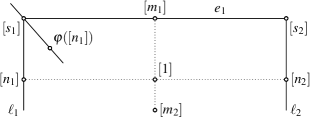
Figure 2: Lines in the proof of Theorem 4 (Lemma 4 and Lemma 5).

Necessity of the first and second condition of Theorem 3 have been proved in the master thesis by Stigger ⁹ by means of Gröbner basis computations. Here, we give an independent proof.

Lemma 4.

The conditions of Theorem 3 are necessary for an RP or PR space that is not a C space.

Proof.

Assuming without loss of generality $[1]\in U$, the constraint variety of an RP chain can be parameterised as

$$R(u,v)=(u-h)(v-\varepsilon p),\quad u\in\mathbb{R}\cup\{\infty\},\ v\in\mathbb{R}\cup\{\infty\}$$ (9)

with a non-zero quaternion $p$ with $p+\overline{p}=0$ and a dual quaternion $h$ that satisfies $h\overline{h}=1$, $h+\overline{h}=0$. Since it is not the constraint variety of a PR chain, the primal part $h^{\prime}$ of $h$ and $p$ do not commute, that is $[h^{\prime}]\neq[p]$.

By the same arguments as in Lemma 2, this constraint variety is a regular quadric: The parameters $u$ and $v$ range in $\mathbb{R}\cup\{\infty\}$ (with $\infty$ corresponding to zero rotation angle or translation distance) but we will also admit complex values for them. Expanding (9) yields $R(u,v)=uv-vh-u\varepsilon p+\varepsilon hp$. We see that the kinematic image of this RP dyad lies in the three-space spanned by $[1]$, $[h]$, $[\varepsilon p]$ and $[\varepsilon hp]=[\varepsilon h^{\prime}p]$ and is a regular quadric.

Clearly, this quadric it contains the line $e_{1}\coloneqq[\varepsilon p]\vee[\varepsilon hp]\subset[\varepsilon\mathbb{H}]$. Moreover, the lines $\ell_{1}$, $\ell_{2}$ parameterised by $R(\pm\mathrm{i},v)$ are conjugate complex null lines. The intersection points $[n_{1}]$, $[n_{2}]$ of these lines with $\tau_{1}$ correspond to $v=\infty$, their intersection points $[s_{1}]$, $[s_{2}]$ with $[\varepsilon\mathbb{H}]$ correspond to $v=0$:

$$n_{1}=\mathrm{i}-h,\ n_{2}=-\mathrm{i}-h,\ s_{1}=-\varepsilon(\mathrm{i}-h)p,\ s_{2}=-\varepsilon(-\mathrm{i}-h)p$$

(Figure 2). In view of Lemma 1 the null line property follows from

$$s_{1}\overline{n_{1}}+n_{1}\overline{s_{1}} =-\varepsilon(\mathrm{i}-h)p(\mathrm{i}-\overline{h})+(\mathrm{i}-h)\overline{p}(-\varepsilon(\mathrm{i}-\overline{h}))$$

$$=-(\mathrm{i}-h)\varepsilon(\underbrace{\overline{p}+p}_{=0})(\mathrm{i}-\overline{h})=0$$

and similar with $\mathrm{i}$ replaced by $-\mathrm{i}$. Moreover $\varphi([\ell_{1}])=\varphi([n_{1}])=[\varepsilon(\mathrm{i}-h^{\prime})]$ and $[s_{1}]=[\varepsilon(\mathrm{i}-h^{\prime})p]$. Because of $[h^{\prime}]\neq[p]$, these points do not coincide and, indeed, span a right ruling of $\mathcal{Y}$.

The statements for PR spaces follow from Theorem 1 by application of the conjugation map $\chi$. It interchanges RP spaces with PR spaces and right rulings with left rulings but fixes the Study quadric and the null cone. ∎

The proof of sufficiency of the conditions in Theorem 3 is, in large parts, a copy of Lemma 3. However, at one point the third condition comes into play.

Lemma 5.

A three-space $U$ that satisfies all conditions of Theorem 3 is a PR or RP space but not a C space.

Proof.

Once more, we assume $[1]\in U$. The intersection of $U$ and $\mathcal{S}$ is a regular quadric $\mathcal{Q}$ that contains the straight line $e_{1}=U\cap[\varepsilon\mathbb{H}]$ and the two conjugate complex null lines $\ell_{1}$, $\ell_{2}$. There exist points $[m_{1}]\in e_{1}$ and $[n_{1}]\in\ell_{1}$ such that $[1]\vee[m_{1}]$ and $[1]\vee[n_{1}]$ are rulings of $\mathcal{Q}$. The points of the line $[1]\vee[m_{1}]$ correspond to translations with fixed direction and the points of $[1]\vee[n_{1}]$ to rotations around a fixed axis. There exists an intersection point $[s_{1}]\coloneqq e_{1}\cap\ell_{1}$ and we have to show that either $[s_{1}]=[m_{1}n_{1}]$ or $[s_{1}]=[n_{1}m_{1}]$. In general, this can be done just as in our proof of Lemma 3: Denote by $m_{2}$ the complex conjugate to $m_{1}$ and by $n_{2}$ the complex conjugate of $n_{1}$. Then $[1]=([m_{1}]\vee[m_{2}])\cap([n_{1}]\vee[n_{2}])$, the quadrilaterals with respective vertices $[m_{1}n_{1}]$, $[m_{2}n_{1}]$, $[m_{2}n_{2}]$, $[m_{1}n_{2}]$ and $[n_{1}m_{1}]$, $[n_{1}m_{2}]$, $[n_{2}m_{2}]$, $[n_{2}m_{1}]$ are contained in $\mathcal{Q}$, and the points $[m_{1}]$, $[n_{1}]$, $[m_{2}]$, and $[n_{2}]$ form a planar quadrilateral. Because the intersection of $[\varepsilon\mathbb{H}]$ and $U$ is not empty, we have to use a projection with three-dimensional centre $Z$ that does not intersect $U$ (and hence differs from $[\varepsilon\mathbb{H}]$) and is such that the plane $[1]\vee[m_{1}]\vee[n_{1}]$ is complementary to the four-spaces

$$[u_{1}]\vee Z,\quad[v_{1}]\vee Z,\quad[u_{2}]\vee Z,\quad[v_{2}]\vee Z$$

when appealing to Lemma 7. Such a choice is possible and then the differences to the proof of Lemma 3 are irrelevant unless $m_{1}$ and $n_{1}$ commute. In this case our argument fails because the two spatial quadrilaterals coincide and we may no longer conclude that the projection of $[s_{1}]$ equals the projection of $[m_{1}n_{1}]$ or of $[n_{1}m_{1}]$. Fortunately, this case is already special enough to allow a straightforward computational treatment.

The dual quaternions $m_{1}$ and $n_{1}$ commute ($m_{1}n_{1}=n_{1}m_{1}$) if the translation direction of $m_{1}$ and the direction of the rotation axis of $n_{1}$ are linearly dependent. Without loss of generality, we may set $m_{1}\coloneqq\varepsilon\mathbf{i}$ and $n_{1}\coloneqq\mathrm{i}+\mathbf{i}$ so that $m_{1}n_{1}=n_{1}m_{1}=\varepsilon(\mathrm{i}\mathbf{i}-1)$. Now $U$ equals the span of $[1]$, $[m_{1}]$, $[n_{1}]$, and $[s_{1}]=[m_{1}n_{1}]=[n_{1}m_{1}]$ but $\varphi(\ell_{1})=\varphi([n_{1}])=[\varepsilon(\mathrm{i}+\mathbf{i})]=[m_{1}n_{1}]$ – a contraction to the assumption that $[s_{1}]$ and $\varphi([n_{1}])$ span a straight line. ∎

Above proof already contains the basic idea for the still missing characterisation of C spaces.

Theorem 4.

A three-space $U\subset P^{7}$ is a C space if and only if it

• intersects the Study quadric in a regular ruled quadric $\mathcal{Q}$,

• contains a pair of conjugate complex null lines $\ell_{1}$, $\ell_{2}$ and a real null line $e_{1}$, and

• satisfies $\varphi(\mathcal{Q})=e_{1}$.

Proof.

Lets assume that $U$ is a C space. Without loss of generality, we may assume that it is spanned by $[1]$, $[m_{1}]=[\varepsilon\mathbf{i}]$, $[n_{1}]=[\mathrm{i}+\mathbf{i}]$ and $[s_{1}]=[m_{1}n_{1}]=\varphi([n_{1}])$. Clearly, it contains the real line $e_{1}=[m_{1}]\vee[s_{1}]$, the null line $\ell_{1}=[s_{1}]\vee[n_{1}]$, and its complex conjugate $\ell_{2}$. A parametric equation for the intersection quadric $\mathcal{Q}$ of $U$ and $\mathcal{S}$ is

$$R(u,v)=(u-n_{1})(v-m_{1}),\quad u\in\mathbb{R}\cup\{\infty\},\ v\in\mathbb{R}\cup\{\infty\}.$$

It is a regular ruled quadric and its fiber projection equals $\varphi(\mathcal{Q})$ is parameterized by $\varepsilon(u-s_{1})$. This is indeed the straight line $e_{1}$.

Conversely, assume that the condition of the theorem hold and, without loss of generality, $[1]\in U$. As in the proof of Lemma 5, we can find points $[m_{1}]$, $[n_{1}]$, $[s_{1}]\in U$ such that $e_{1}=[m_{1}]\vee[s_{1}]$, $\ell_{1}=[n_{1}]\vee[s_{1}]$, and the lines $[1]\vee[m_{1}]$ and $[1]\vee[n_{1}]$ are rulings of $\mathcal{Q}$. After a suitable choice of coordinates, we may assume $n_{1}=\mathrm{i}+\mathbf{i}$ whence

$$e_{1}=\varphi([1])\vee\varphi([n_{1}])=[\varepsilon]\vee[\varepsilon(\mathrm{i}+\mathbf{i})]=[\varepsilon]\vee[\varepsilon\mathbf{i}].$$

But then $[m_{1}]=[\varepsilon\mathbf{i}]$ because $[m_{1}]\in e_{1}$ and $[1]\vee[m_{1}]$ is contained in $\mathcal{S}$. In particular, $[m_{1}n_{1}]=[n_{1}m_{1}]=[\varepsilon(\mathrm{i}\mathbf{i}-1)]=[\varepsilon(\mathrm{i}+\mathbf{i})]$. Moreover, there exist scalars $\alpha$ and $\beta$ such that $s_{1}=\varepsilon(\alpha+\beta\mathbf{i})$. The condition $n_{1}\overline{s_{1}}+s_{1}\overline{n_{1}}=0$ implies $\alpha=\mathrm{i}\beta$ so that $[s_{1}]=[\varepsilon(\mathrm{i}+\mathbf{i})]=[m_{1}n_{1}]=[n_{1}m_{1}]$ and $U$ is indeed a C space. ∎

6 Extended Kinematic Mapping and Straight Lines

In this section we illustrate the usefulness of Theorem 4 at hand of an example. In Pfurner et al. ⁵ the authors consider the map (1) but without imposing the Study condition (“extended kinematic map”). The action of a dual quaternion on points is still a rigid body transformation but the map is no longer an injection. Pfurner et al. (2016) show that the fibers of (1) (the set of pre-images of a fixed rigid body displacement) is a straight line. More precisely, the fiber incident with a point $[p]=[p^{\prime}+\varepsilon p^{\prime\prime}]\in P^{7}\setminus[\varepsilon\mathbb{H}]$ is the straight line $[p^{\prime}+\varepsilon p^{\prime\prime}]\vee[\varepsilon p^{\prime\prime}]=\varphi([p])$. This line intersects the Study quadric in $[\varepsilon p]$ and one further point which gives the corresponding displacement in the classical kinematic map (which also the underlying concept in this paper).

Pfurner et al. (2016) also mention that the motion corresponding to a generic straight line in $P^{7}$ is a Darboux motion ^{1; 8}, that is, the motion obtained by composing a planar elliptic motion with a harmonic oscillation in orthogonal direction. This is fairly straightforward to see. By virtue of (1), all trajectories are rational curves degree two or less which already limits possible candidates to Darboux motions, rotations with fixed axis, and curvilinear translations along rational curves of degree two or less.

We will now prove that the motion of a generic straight line $\ell$ is actually a vertical Darboux motion. In this limiting case of the generic Darboux motion the elliptic translation is replaced by a rotation with fixed axis. Our proof is based on the fact that the three-space spanned by $\ell$ and its fiber $\varphi(\ell)$ is a C space.

Theorem 5.

If a straight line $\ell\subset P^{7}$ contains a point $[p]\notin[\varepsilon\mathbb{H}]$ and is neither contained in the null cone $\mathcal{N}$ nor in the four-dimensional subspace $[T]\coloneqq[p]\vee[\varepsilon\mathbb{H}]$, the span of $\ell$ and $\varphi(\ell)$ is a C space.

Proof.

Without loss of generality we assume $[p]=[1]$. Then $[T]$ is the space of all translations. The straight line $\ell$ is neither contained in nor tangent to the null cone $\mathcal{N}$ (because it is real and does not intersect $[\varepsilon\mathbb{H}]$). Hence, it intersects $\mathcal{N}$ in two points $[a]=[a^{\prime}+\varepsilon a^{\prime\prime}]$, $[b]=[b^{\prime}+\varepsilon b^{\prime\prime}]$. They satisfy the null cone condition $a^{\prime}\overline{a^{\prime}}=b^{\prime}\overline{b^{\prime}}=0$. Because $[1]\in[a]\vee[b]$, we may write $b=\overline{a^{\prime}}-\varepsilon a^{\prime\prime}$. Note that $a$ and $b$ are complex conjugates but we will not make direct use of this, thus avoiding possible confusion arising from mixing of complex and quaternion conjugation.

If the vectors $a^{\prime}$ and $\overline{a^{\prime}}$ are linearly dependent, there exists a linear combination $\varepsilon c^{\prime\prime}$ of $a$ and $b$ with $c^{\prime\prime}\neq 0$. But then $[1]\neq[\varepsilon c^{\prime\prime}]\in[T]$ and, contrary to our assumption, $\ell=[1]\vee[\varepsilon c^{\prime\prime}]\subset[T]$. Hence, $a^{\prime}$ and $\overline{a^{\prime}}$ are linearly independent. This implies that the points $[a]=[a^{\prime}+\varepsilon a^{\prime\prime}]$, $[b]=[\overline{a^{\prime}}-\varepsilon a^{\prime\prime}]$, $\varphi([a])=[\varepsilon a^{\prime}]$, and $\varphi([b])=[\varepsilon\overline{a^{\prime}}]$ span a three-dimensional space $U$.

Now we compute the intersection of $U$ with $\mathcal{S}$ and $\mathcal{N}$. We set $x=\alpha a+\beta\overline{a}+\varepsilon(\gamma a^{\prime}+\delta\overline{a^{\prime}})$ and solve the equation $x\overline{x}=0$ for $[\alpha,\beta,\gamma,\delta]$. The left-hand side is a dual number. Equating its primal part with zero yields

$$\alpha\beta({a^{\prime}}^{2}+\overline{a^{\prime}}^{2})=0.$$

Note that $f\coloneqq{a^{\prime}}^{2}+\overline{a^{\prime}}^{2}$ is a real number and it is different from zero because of linear independence of $a^{\prime}$ and $\overline{a^{\prime}}$. Hence $\alpha=0$ or $\beta=0$. We further abbreviate

$$g_{1}\coloneqq a^{\prime}\overline{a^{\prime\prime}}+a^{\prime\prime}\overline{a^{\prime}},\quad g_{2}\coloneqq\overline{a^{\prime}}\,\overline{a^{\prime\prime}}+a^{\prime\prime}a^{\prime}$$

(these are real numbers as well) and equate the dual part of $x\overline{x}=0$ with zero:

$$(\alpha\delta+\beta\gamma)f+\alpha(\alpha-\beta)g_{1}+\beta(\alpha-\beta)g_{2}=0$$

In case of $\beta=0$, this boils down to

$$\alpha(\delta f+\alpha g_{1})=0$$

while we get

$$\beta(\gamma f-\beta g_{2})=0$$

if $\alpha=0$. From these considerations we infer that $U\cap\mathcal{S}\cap\mathcal{N}$ consists of precisely three straight lines: The line $e_{1}$ given by $[\alpha,\beta,\gamma,\delta]=[0,0,\gamma,\delta]$ which is contained in the exceptional generator $[\varepsilon\mathbb{H}]$, and the two lines $\ell_{1}$, $\ell_{2}$ given by

$$[\alpha,\beta,\gamma,\delta]=[-f,0,\gamma,g_{1}],\quad\text{and}\quad[\alpha,\beta,\gamma,\delta]=[0,f,g_{2},\delta]$$

respectively. Because of $f\neq 0$, the lines $\ell_{1}$ and $\ell_{2}$ do not intersect and they are complex conjugates by construction. This already implies that $U\cap\mathcal{S}$ is a ruled quadric but neither a quadratic cone nor a double plane (but we still have to argue that it is not a pair of planes).

Figure 3: Lines in the proof of Theorem 5.

For $\alpha=\beta=0$ and $\gamma=\infty$ or $\delta=\infty$ we obtain the intersection points

$$[s_{1}]=[\varepsilon a^{\prime}]\quad\text{and}\quad[s_{2}]=[\varepsilon\overline{a^{\prime}}]$$ (10)

of $\ell_{1}$ and $\ell_{2}$, respectively, with $e_{1}$. There is a unique line $n$ through $[1]$ that intersects both $\ell_{1}$ and $\ell_{2}$. Its intersection points $[n_{1}]$, $[n_{2}]$ with $\ell_{1}$ and $\ell_{2}$, respectively, are given by

$$[\alpha,\beta,\gamma,\delta]=[-f,0,g_{2},g_{1}]\quad\text{and}\quad[\alpha,\beta,\gamma,\delta]=[0,f,g_{2},g_{1}].$$

The line $[n_{1}]\vee[n_{2}]$ is a fourth ruling in the intersection of $U$ and $\mathcal{S}$ and does not intersect $[e_{1}]$. Hence $U$ and $\mathcal{S}$ cannot intersect in a pair of planes.

The quadric $\mathcal{Q}=\mathcal{S}\cap U$ is given by the equations $x=\alpha a+\beta\overline{a}+\varepsilon(\gamma a^{\prime}+\delta\overline{a^{\prime}})$ where the parameters $\alpha$, $\beta$, $\gamma$, and $\delta$ satisfy $\alpha\delta+\beta\gamma=0$. From this we see that that its fiber projection is given by $[\varepsilon(\alpha a^{\prime}+\beta\overline{a^{\prime}})]$. It, indeed, coincides with $e_{1}$ so that also the last condition of Theorem 4 is fulfilled. ∎

Corollary 1.

A straight line $\ell$ satisfying the assumptions of Theorem 5 corresponds, via (1), to a vertical Darboux motion.

Proof.

Since the map (1) generically doubles the degree, the trajectories of the motion in question are at most quadratic and the motion itself is either a curvilinear translation along a curve of degree two or less, the rotation about a fixed axis or a Darboux motion. Pure translations are excluded by the assumptions of Theorem 5, non-vertical Darboux motions by its conclusion. ∎

Remark 2.

Corollary 1 is also valid for straight lines contained in the Study quadric $\mathcal{S}$ unless they intersect the exceptional generator $[\varepsilon\mathbb{H}]$. These lines are known to describe rotations about a fixed axis (Selig 2005, Section 11.2) ², that is, a vertical Darboux motion with zero amplitude. In this sense, we may say that all straight lines in extended kinematic image space that intersect the null cone in two distinct points describe a vertical Darboux motion.

7 Conclusion

We provided necessary and sufficient geometric conditions on the transformation group induced by coordinate changes in the fixed and moving frame and on the kinematic image of 2R, RP, and PR dyads. While many properties of these objects are already known, sufficiency of certain collections of conditions seems to be new. We payed proper attention to the case of commuting joints (which is trivial for RR dyads), highlighted the role of left and right rulings, and introduced the fiber projectivity. It is important in our characterisation of RP and PR spaces but also for the kinematic images of Darboux motions, as illustrated in Example 1 and Section 6.

Appendix A Auxiliary results

In this appendix we prove two technical results of purely projective nature and with no direct relations to kinematics. The formulation of Lemma 6 could be simplified but in its present form its application in the proof of Lemma 7 is apparent.

Lemma 6.

Given a three-space $E\subset P^{7}$ and four points $[u^{\prime}_{1}]$, $[v^{\prime}_{1}]$, $[u^{\prime}_{2}]$, $[v^{\prime}_{2}]$ that span a three-space $F\subset P^{7}$ with $E\cap F=\varnothing$, set $U_{1}\coloneqq[u^{\prime}_{1}]\vee E$, $V_{1}\coloneqq[v^{\prime}_{1}]\vee E$, $U_{2}\coloneqq[u^{\prime}_{2}]\vee E$, $V_{2}\coloneqq[v^{\prime}_{2}]\vee E$ and consider four projections

$$\zeta_{1}\colon U_{1}\to V_{1},\quad\eta_{1}\colon V_{1}\to U_{2},\quad\zeta_{2}\colon U_{2}\to V_{2},\quad\eta_{2}\colon V_{2}\to U_{1}$$

with respective centres $[m_{1}]$, $[n_{1}]$, $[m_{2}]$, and $[n_{2}]$. If the centres are pairwise different and span a plane $L$ that is complementary to $U_{1}$, $V_{1}$, $U_{2}$, and $V_{2}$, respectively, the composition $\eta_{2}\circ\zeta_{2}\circ\eta_{1}\circ\zeta_{1}$ of the four projections is the identity.

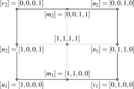
Figure 4: Projective coordinates in the proof of Lemma 6 (four trailing zeros are omitted).

Proof.

Note that $\dim U_{1}\vee V_{1}=5$ so that the projection $\zeta_{1}$ (and also $\eta_{1}$, $\zeta_{2}$, $\eta_{2}$) from a suitable point is well defined. Take an arbitrary point $[u_{1}]\in U_{1}$ but not in $E$ and set $[v_{1}]\coloneqq\zeta_{1}([u_{1}])$, $[u_{2}]\coloneqq\eta_{1}([v_{1}])$, $[v_{2}]\coloneqq\zeta_{2}([u_{2}])$. Then the projective space $G\coloneqq[u_{1}]\vee[v_{1}]\vee[u_{2}]\vee[v_{2}]=[u_{1}]\vee[m_{1}]\vee[n_{1}]\vee[m_{2}]\vee[n_{2}]$ (Figure 4) is of dimension three and does not intersect $E$ because of the dimension formula

$$\dim(G\cap E) =\dim G+\dim E-\dim(G\vee E)$$

$$=3+3-\dim([u_{1}]\vee L\vee E)=3+3-7=-1.$$

Therefore, we may take $[u_{1}]$, $[v_{1}]$, $[u_{2}]$ and $[v_{2}]$ in that order as base points of a projective coordinate system in $G$ and complement them by four further base points in $E$ and a suitable unit point to a projective coordinate system of $P^{7}$. We select the unit point such that its projection into $G$ from $E$ gives $([m_{1}]\vee[m_{2}])\cap([n_{1}]\vee[n_{2}])$. Then, the projection centres are

$$[m_{1}]=[1,1,0,0,0,0,0,0],\quad[n_{1}]=[0,1,1,0,0,0,0,0],$$

$$[m_{2}]=[0,0,1,1,0,0,0,0],\quad[n_{2}]=[1,0,0,1,0,0,0,0].$$

We pick an arbitrary point $h_{2}\coloneqq[x_{0},0,0,0,x_{4},x_{5},x_{6},x_{7}]\in U_{1}$ and compute

$$\zeta_{1}(h_{2}) =[0,-x_{0},0,0,x_{4},x_{5},x_{6},x_{7}]\eqqcolon z_{1},$$

$$\eta_{1}(z_{1}) =[0,0,x_{0},0,x_{4},x_{5},x_{6},x_{7}]\eqqcolon h_{1},$$

$$\zeta_{2}(h_{1}) =[0,0,0,-x_{0},x_{4},x_{5},x_{6},x_{7}]\eqqcolon z_{2},$$

$$\eta_{2}(z_{2}) =[x_{0},0,0,0,x_{4},x_{5},x_{6},x_{7}]=h_{2}.$$

This concludes the proof. ∎

Lemma 7.

Let $E$, $F\subset P^{7}$ be non-intersecting three-spaces, the latter spanned by points $[u^{\prime}_{1}]$, $[v^{\prime}_{1}]$, $[u^{\prime}_{2}]$, $[v^{\prime}_{2}]$. Consider further a regular quadric $\mathcal{Q}$ containing $E$ and four vertices $[m_{1}]$, $[n_{1}]$, $[m_{2}]$, $[n_{2}]\in\mathcal{Q}$ of a quadrilateral in a plane $L$ that is complementary to

$$E\vee[u^{\prime}_{1}],\quad E\vee[v^{\prime}_{1}],\quad E\vee[u^{\prime}_{2}],\quad\text{and}\quad E\vee[v^{\prime}_{2}].$$

Then there exists a unique spatial quadrilateral with vertices $[u_{1}]$, $[v_{1}]$, $[u_{2}]$, $[v_{2}]$ that is contained in $\mathcal{Q}$, whose sides $[u_{1}]\vee[v_{1}]$, $[v_{1}]\vee[u_{2}]$, $[u_{2}]\vee[v_{2}]$, $[v_{2}]\vee[u_{1}]$ are, in that order, incident with $[m_{1}]$, $[n_{1}]$, $[m_{2}]$, $[n_{2}]$ and whose projection from $E$ into $F$ is the quadrilateral with vertices $[u^{\prime}_{1}]$, $[v^{\prime}_{1}]$, $[u^{\prime}_{2}]$, and $[v^{\prime}_{2}]$.

Proof.

Denote the quadratic form associated to $\mathcal{Q}$ by $\omega$. Given $[u^{\prime}_{1}]$, $[v^{\prime}_{1}]$, $[u^{\prime}_{2}]$, $[v^{\prime}_{2}]$, we have to reconstruct $[u_{1}]$, $[v_{1}]$, $[u_{2}]$, $[v_{2}]$ subject to the constraints

$$\omega(u_{i},u_{i})=\omega(v_{i},v_{i})=\omega(u_{i},v_{j})=0,\quad i,j\in\{1,2\}$$ (11)

and

$$\begin{gathered}\in[u_{1}]\vee[v_{1}],\quad[n_{1}]\in[v_{1}]\vee[u_{2}],\\ [m_{2}]\in[u_{2}]\vee[v_{2}],\quad[n_{2}]\in[v_{2}]\vee[u_{1}].\end{gathered}$$ (12)

If $[u_{1}]$ is given, we find $[v_{1}]$ by projecting $[u_{1}]$ from centre $[m_{1}]$ onto $E\vee[v^{\prime}_{1}]$. Lemma 6 tells us that we can find $[u_{2}]$ and $[v_{2}]$ in similar manner such that (12) is satisfied. Then, some of the conditions in (11) become redundant and it is sufficient to consider only

$$\omega(u_{1},u_{1})=\omega(v_{1},v_{1})=\omega(u_{2},u_{2})=\omega(v_{2},v_{2})=0.$$ (13)

In a projective coordinate system with base points $[u^{\prime}_{1}]$, $[v^{\prime}_{1}]$, $[u^{\prime}_{2}]$, $[v^{\prime}_{2}]\in F$ and further base points in $E$, the quadratic form $\omega$ of the quadric $\mathcal{Q}$ is described by a matrix of the shape

$$\begin{bmatrix}A&B\\ B&O\end{bmatrix}$$

where $A$, $B$ and $O$ are matrices of dimension $4\times 4$, $O$ is the zero matrix and $B$ is regular. Now (13) gives rise to a linear system for the unknown coordinates of $[u_{1}]$, $[v_{1}]$, $[u_{2}]$, and $[v_{2}]$. We have

$$v_{1} =u_{1}+\zeta_{1}m_{1},$$

$$u_{2} =v_{1}+\eta_{1}n_{1}=u_{1}+\zeta_{1}m_{1}+\eta_{1}n_{1},$$

$$v_{2} =u_{2}+\zeta_{2}m_{2}=u_{1}+\zeta_{1}m_{1}+\eta_{1}n_{1}+\zeta_{2}m_{2}$$

with certain scalars $\zeta_{1}$, $\eta_{1}$, $\zeta_{2}$ that can be computed from $u^{\prime}_{1}$, $v^{\prime}_{1}$, $u^{\prime}_{2}$, $v^{\prime}_{2}$ and $m_{1}$, $n_{1}$, $m_{2}$, $n_{2}$ alone. Now we write $[u_{1}]=[1,0,0,0,x_{0},x_{1}x_{2},x_{3}]$ with unknown $x_{0}$, $x_{1}$, $x_{2}$, $x_{3}$. Then, (13) yields

$$0 =[1,0,0,0]\cdot B[x_{0},x_{1},x_{2},x_{3}]^{\intercal},$$ (14)

$$0 =[0,1,0,0]\cdot B([x_{0},x_{1},x_{2},x_{3}]+\zeta_{1}m^{\prime\prime}_{1})^{\intercal},$$

$$0 =[0,0,1,0]\cdot B([x_{0},x_{1},x_{2},x_{3}]+\zeta_{1}m^{\prime\prime}_{1}+\eta_{1}n^{\prime\prime}_{1})^{\intercal},$$

$$0 =[0,0,0,1]\cdot B([x_{0},x_{1},x_{2},x_{3}]+\zeta_{1}m^{\prime\prime}_{1}+\eta_{1}n^{\prime\prime}_{1}+\zeta_{2}m^{\prime\prime}_{2})^{\intercal}$$

where the double prime denotes projection on the last four coordinates. (14) is a linear system for $x_{0}$, $x_{1}$, $x_{2}$, $x_{3}$ with regular coefficient matrix $B$. Hence, the solution is unique. ∎

References

- 1 O. Bottema and B. Roth: Theoretical Kinematics (Dover Publications, 1990).
- 2 J. Selig: Geometric Fundamentals of Robotics. Monographs in Computer Science (Springer, 2005), 2nd edition.
- 3 M. Husty and H.-P. Schröcker: “Kinematics and algebraic geometry.” In J. M. McCarthy, editor, “21st Century Kinematics. The 2012 NSF Workshop,” 85–123 (Springer, London, 2012).
- 4 D. Klawitter: Clifford Algebras. Geometric Modelling and Chain Geometries with Application in Kinematics (Springer Spektrum, 2015).
- 5 M. Pfurner, H.-P. Schröcker, and M. Husty: “Path planning in kinematic image space without the Study condition.” In J. Lenarčič and J.-P. Merlet, editors, “Proceedings of Advances in Robot Kinematics,” (2016). URL https://hal.archives-ouvertes.fr/hal-01339423.
- 6 T.-D. Rad and H.-P. Schröcker: “The kinematic image of 2R dyads and exact synthesis of 5R linkages.” In “Proceedings of the IMA Conference on Mathematics of Robotics,” (2015). ISBN 978-0-90-509133-4.
- 7 H. S. M. Coxeter: Non-Euclidean Geometry (Cambride Univesristy Press, 1998), 6th edition.
- 8 Z. Li, J. Schicho, and H.-P. Schröcker: “7R Darboux linkages by factorization of motion polynomials.” In S.-H. Chang, editor, “Proceedings of the 14th IFToMM World Congress,” (2015).
- 9 T. Stigger: Algebraic constraint equations of simple kinematic chains. Master thesis, University of Innsbruck (2015).