Varying the resolution of the Rouse model on temporal and spatial scales: application to multiscale modelling of DNA dynamics

Abstract

A multi-resolution bead-spring model for polymer dynamics is developed as a generalization of the Rouse model. A polymer chain is described using beads of variable sizes connected by springs with variable spring constants. A numerical scheme which can use different timesteps to advance the positions of different beads is presented and analyzed. The position of a particular bead is only updated at integer multiples of the timesteps associated with its connecting springs. This approach extends the Rouse model to a multiscale model on both spatial and temporal scales, allowing simulations of localized regions of a polymer chain with high spatial and temporal resolution, while using a coarser modelling approach to describe the rest of the polymer chain. A method for changing the model resolution on-the-fly is developed using the Metropolis-Hastings algorithm. It is shown that this approach maintains key statistics of the end-to-end distance and diffusion of the polymer filament and makes computational savings when applied to a model for the binding of a protein to the DNA filament.

mmsxxxxxxxx–x

1 Introduction

Over the past 70 years, there have been multiple attempts to dynamically model the movement of polymer chains with Brownian dynamics [37, 38, 47, 24], which have more recently been used as a model for DNA filament dynamics [2]. One of the first and simplest descriptions was given as the Rouse model [38], which is a bead-spring model [2], where the continuous filament is modelled at a mesoscopic scale with beads connected by springs. The only forces exerted on beads are spring forces from adjacent springs, as well as Gaussian noise. Hydrodynamic forces between beads and excluded volume effects are neglected in the model in favour of simplicity and computational speed, but the model manages to agree with several properties of polymer chains from experiments [24, 34]. Other models exist, for example the Zimm model introduces hydrodynamic forces [47] between beads, or bending potentials can be introduced to form a wormlike chain and give a notion of persistence length [1], see, for example, review article [2] or books [7, 6] on this subject.

Most of the aforementioned models consider the filament on only a single scale. In some applications, a modeller is interested in a relatively small region of a complex system. Then it is often possible to use a hybrid model which is more accurate in the region of interest, and couple this with a model which is more computationally efficient in the rest of the simulated domain [13, 8, 9]. An application area for hybrid models of polymer chains is binding of a protein to the DNA filament, which we study in this paper. The model which we have created uses Rouse dynamics for a chain of DNA, along with a freely diffusing particle to represent a binding protein. As the protein approaches the DNA, we increase the resolution in the nearby DNA filament to increase accuracy of our simulations, whilst keeping them computationally efficient.

In this paper we use the Rouse model for analysis due to its mathematical tractability and small computational load. Such a model is applicable to modelling DNA dynamics when we consider relatively low resolutions, when hydrodynamic forces are negligible and persistence length is significantly shorter than the Kuhn length between each bead [2]. The situation becomes more complicated when we consider DNA modelling at higher spatial resolutions.

Inside the cell nucleus, genetic information is stored within strands of long and thin DNA fibres, which are separated into chromosomes. These DNA fibres are folded into structures related to their function. Different genes can be enhanced or inhibited depending upon this structure [12]. Folding also minimises space taken up in the cell by DNA [21], and can be unfolded when required by the cell for different stages in the cell cycle or to alter gene expression. The folding of DNA occurs on multiple scales. On a microscopic scale, DNA is wrapped around histone proteins to form the nucleosome structure [45]. This in turn gets folded into a chromatin fibre which gets packaged into progressively higher order structures until we reach the level of the entire chromosome [12]. The finer points of how the nucleosome packing occurs on the chromatin fibre and how these are then packaged into higher-order structures is still a subject of much debate, with long-held views regarding mesoscopic helical fibres becoming less fashionable in favour of more irregular structures in vivo [28].

In the most compact form of chromatin, many areas of DNA are not reachable for vital reactions such as transcription [12]. One potential explanation to how this is overcome by the cell is to position target DNA segments at the surface of condensed domains when it is needed [27, 5], so that transcription factors can find expressed genes without having to fit into these tightly-packed structures. This complexity is not captured by the multiscale model of protein binding presented in this paper. However, if one uses the developed refinement of the Rouse model together with a more detailed modelling approach in a small region of DNA next to the binding protein, then such a hybrid model can be used to study the effects of microscopic details on processes over system-level spatial and temporal scales. When taking this multiscale approach, it is necessary to understand the error from including the less accurate model in the hybrid model and how the accuracy of the method depends on its parameters. These are the main questions studied in this paper.

The rest of the paper is organized as follows. In Section 2, we introduce a multi-resolution bead-spring model which generalizes the Rouse model. We also introduce a discretized version of this model which enables the use of different timesteps in different spatial regions. In Section 3, we analyze the main properties of the multi-resolution bead-spring model. We prove two main lemmas giving formulas for the diffusion constant and the end-to-end distance. We also study the appropriate choice of timesteps for numerical simulations of the model and support our analysis by the results of illustrative computer simulations. Our main application area is studied in Section 4 where we present and analyze a DNA binding model. We develop a method to increase the resolution in existing segments on-the-fly using the Metropolis-Hastings algorithm. In Section 5, we conclude our paper by discussing possible extensions of the presented multiscale approach (by including more detailed models of DNA dynamics) and other multiscale methods developed in the literature.

2 Multi-resolution bead-spring model

We generalize the classical Rouse bead-spring polymer model [38] to include beads of variable sizes and springs with variable spring constants. In Definition 1, we formulate the evolution equation for this model as a system of stochastic differential equations (SDEs). We will also introduce a discretized version of this model in Algorithm 1, which will be useful in Sections 3 and 4 where we use the multi-resolution bead-spring model to develop and analyze multiscale models for DNA dynamics.

Definition 1.

Let $N>1$ be a positive integer. A multi-resolution bead-spring polymer of size $N$ consists of a chain of $N$ beads of radius $\sigma_{n}$, for $n=1,2,\dots,N$, connected by $N-1$ springs which are characterized by their spring constants $k_{n}$, for $n=1,2,\dots,N-1$. The positions $\mathbf{r}_{n}\equiv\mathbf{r}_{n}(t)=[r_{n,1}(t),r_{n,2}(t),r_{n,3}(t)]$ of beads evolve according to the system of SDEs (for $n=1,2,\dots,N$)

$$\zeta_{n}\,\mbox{{\rm d}}\mathbf{r}_{n}=\Big{(}k_{n-1}\mathbf{r}_{n-1}(t)-(k_{n-1}+k_{n})\mathbf{r}_{n}(t)+k_{n}\mathbf{r}_{n+1}(t)\Big{)}\,\mbox{{\rm d}}t+\sqrt{2k_{B}T\zeta_{n}}\;\mbox{{\rm d}}{\mathbf{W}}_{n},$$ (1)

where $\zeta_{n}=6\pi\eta\sigma_{n}$ is the frictional drag coefficient of the $n$-th bead given by Stokes’ Theorem, $\eta$ is the solvent viscosity, $\mbox{{\rm d}}{\mathbf{W}}_{n}\equiv[\mbox{{\rm d}}W_{n,1},\mbox{{\rm d}}W_{n,2},\mbox{{\rm d}}W_{n,3}]$ is a Wiener process, $T$ is absolute temperature, $k_{B}$ is Boltzmann’s constant and we assume that each spring constant $k_{n}$ can be equivalently expressed in terms of the corresponding Kuhn length $b_{n}$ by

$$k_{n}=\frac{3k_{B}T}{b_{n}^{2}},\qquad\mbox{for}\quad n=1,2,\dots,N-1.$$

We assume that the behaviour of boundary beads (for $n=1$ and $n=N$) is also given by equation $(\ref{SDEdef})$ simplified by postulating $\mathbf{r}_{0}(t)=\mathbf{r}_{1}(t)$ and $\mathbf{r}_{N+1}(t)=\mathbf{r}_{N}(t).$

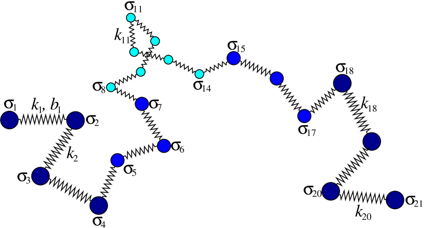
Fig. 1: A schematic of the multi-resolution bead-spring model for $N=21.$

In Figure 1, we schematically illustrate a multi-resolution bead-spring polymer for $N=21$. The region between the $8$-th and the $14$-th bead is described with the highest resolution by considering smaller beads and springs with larger spring constants (or equivalently with smaller Kuhn lengths). The scalings of different parameters in Definition 1 are chosen so that we recover the classical Rouse model [38] if we assume $\sigma_{1}=\sigma_{2}=\dots=\sigma_{N}=\sigma$ and $b_{1}=b_{2}=\dots=b_{N-1}=b$. Then equation (1) simplifies to

$$\zeta\,\mbox{{\rm d}}\mathbf{r}_{n}=k\,\Big{(}\mathbf{r}_{n-1}(t)-2\mathbf{r}_{n}(t)+\mathbf{r}_{n+1}(t)\Big{)}\,\mbox{{\rm d}}t+\sqrt{2k_{B}T\zeta}\;\mbox{{\rm d}}{\mathbf{W}}_{n},$$ (2)

where $\zeta=6\pi\eta\sigma$, $k=3k_{B}T/b^{2}$ and we again define $\mathbf{r}_{0}(t)=\mathbf{r}_{1}(t)$ and $\mathbf{r}_{N+1}(t)=\mathbf{r}_{N}(t)$ in equations for boundary beads. In the polymer physics literature [7], the Rouse model (2) is equivalently written as

$$\zeta\frac{d\mathbf{r}_{n}}{dt}(t)=k\,\Big{(}\mathbf{r}_{n-1}(t)-2\mathbf{r}_{n}(t)+\mathbf{r}_{n+1}(t)\Big{)}+\mathbf{f}_{n}(t),$$ (3)

where random thermal noises $\mathbf{f}_{n}(t)$ exerted on the beads from Brownian motion are characterized by the moments [7]

$$\langle\mathbf{f}_{n}(t)\rangle=\mathbf{0},\qquad\langle f_{n,i}(t)f_{m,j}(t^{\prime})\rangle=2\zeta k_{B}T\delta_{nm}\delta_{ij}\delta(t-t^{\prime}),$$ (4)

where $n,m=1,2,\ldots,N$ and $i,j\in\{1,2,3\}$. For the remainder of this paper, we will use the SDE notation as given in (2), because we will often study numerical schemes for simulating polymer dynamics models. The simplest discretization of (2) is given by the Euler-Maruyama method [20], which uses the finite timestep $\Delta t$ and calculates the position vector $\mathbf{r}_{n}^{t}$ of the $n$-th bead, $n=1,2,\ldots,N$, at discretised time $t$ by

$$\mathbf{r}_{n}^{t}=\mathbf{r}_{n}^{t-\Delta t}+\frac{k}{\zeta}\left(\mathbf{r}_{n-1}^{t-\Delta t}-2\,\mathbf{r}_{n}^{t-\Delta t}+\mathbf{r}_{n+1}^{t-\Delta t}\right)\,\Delta t+\sqrt{\frac{2k_{B}T}{\zeta}\Delta t}\ \bm{\xi}_{n}$$ (5)

for $\bm{\xi}_{n}=(\xi_{n,1},\xi_{n,2},\xi_{n,3})$, where $\xi_{n,i}$ is normally distributed random variable with zero mean and unit variance (i.e. $\xi_{n,i}\sim\mathcal{N}(0,1)$) for $i=1,2,3$. In order to discretize the multi-resolution bead-spring model, we allow for variable timesteps.

Definition 2.

Let $\Delta t>0$ and let $j_{n}$, $n=1,2,\dots,N-1,$ be positive integers such that $j_{n-1}\mid j_{n}$ or $j_{n}\mid j_{n-1}$ for $n=2,3,\dots,N-1$. Let us assume that at least one of the values of $j_{n}$ is equal to 1. We define $\Delta t_{n}=j_{n}\Delta t$ for $n=1,2,\dots,N-1$ and we call $\Delta t_{n}$ a timestep associated with the $n$-th spring.

Definition 2 specifies that all timesteps must be integer multiples of the smallest timestep $\Delta t$. The timesteps associated with two adjacent springs are also multiples of each other. The time evolution of the multi-resolution bead-spring model is computed at integer multiples of $\Delta t$. One iteration of the algorithm is shown in Algorithm 1. The position of the $n$-th bead is updated at integer multiples of $\min\{j_{n-1},j_{n}\}\Delta t=\min\{\Delta t_{n-1},\Delta t_{n}\}$ by calculating the random displacement due to Brownian motion, with displacement caused by springs attached to the bead also updated at integer multiples of the timesteps associated with each spring, i.e. $\Delta t_{n-1}$ or $\Delta t_{n}.$ Considering the situation that all beads, springs and timesteps are the same, then one can easily deduce the following result.

Update positions of internal beads which are connected to two springs:

for $n=2,3,\dots,N-1$ do

       if $\min\{j_{n-1},j_{n}\}\mid i$ then

             Put $\mathbf{r}_{n}^{i\Delta t}:=\mathbf{r}_{n}^{(i-1)\Delta t}+\sqrt{\displaystyle\frac{2k_{B}T}{\zeta_{n}}\min\{j_{n-1},j_{n}\}\Delta t}\,\bm{\xi}_{n}^{i}$ where $\bm{\xi}_{n}^{i}$ is a vector

             of random numbers sampled from $\bm{\xi}_{n}^{i}\sim[\mathcal{N}(0,1),\mathcal{N}(0,1),\mathcal{N}(0,1)]$.

             if $j_{n-1}\mid i$ then

                   Put $\mathbf{r}_{n}^{i\Delta t}:=\mathbf{r}_{n}^{i\Delta t}+\displaystyle\frac{k_{n-1}}{\zeta_{n}}\left(\mathbf{r}_{n-1}^{(i-j_{n-1})\Delta t}-\mathbf{r}_{n}^{(i-j_{n-1})\Delta t}\right)\,\Delta t_{n-1}$.

             end if

            if $j_{n}\mid i$ then

                   Put $\mathbf{r}_{n}^{i\Delta t}:=\mathbf{r}_{n}^{i\Delta t}+\displaystyle\frac{k_{n}}{\zeta_{n}}\left(\mathbf{r}_{n+1}^{(i-j_{n})\Delta t}-\mathbf{r}_{n}^{(i-j_{n})\Delta t}\right)\,\Delta t_{n}$.

             end if

            

      else

            Put $\mathbf{r}_{n}^{i\Delta t}:=\mathbf{r}_{n}^{(i-1)\Delta t}$.

       end if

      

end for

Update of the first bead:

if $j_{1}\mid i$ then

       Put $\mathbf{r}_{1}^{i\Delta t}:=\mathbf{r}_{1}^{(i-1)\Delta t}+\displaystyle\frac{k_{1}}{\zeta_{1}}\left(\mathbf{r}_{2}^{(i-j_{1})\Delta t}-\mathbf{r}_{1}^{(i-j_{1})\Delta t}\right)\,\Delta t_{1}+\mbox{$\sqrt{\displaystyle\frac{2k_{B}T}{\zeta_{1}}\Delta t_{1}}$}\,\bm{\xi}_{1}^{i}$

       where $\bm{\xi}_{1}^{i}\sim[\mathcal{N}(0,1),\mathcal{N}(0,1),\mathcal{N}(0,1)]$.

else

      Put $\mathbf{r}_{1}^{i\Delta t}:=\mathbf{r}_{1}^{(i-1)\Delta t}$.

end if

Update of the last bead:

if $j_{N-1}\mid i$ then

       Put $\mathbf{r}_{N}^{i\Delta t}:=\mathbf{r}_{N}^{(i-1)\Delta t}+\displaystyle\frac{k_{N-1}}{\zeta_{N}}\left(\mathbf{r}_{N-1}^{(i-j_{N-1})\Delta t}-\mathbf{r}_{N}^{(i-j_{N-1})\Delta t}\right)\,\Delta t_{N-1}$

                    $+\,\sqrt{\displaystyle\frac{2k_{B}T}{\zeta_{N}}\Delta t_{N-1}}\,\bm{\xi}_{N}^{i}$ where $\bm{\xi}_{N}^{i}\sim[\mathcal{N}(0,1),\mathcal{N}(0,1),\mathcal{N}(0,1)]$.

else

      Put $\mathbf{r}_{N}^{i\Delta t}:=\mathbf{r}_{N}^{(i-1)\Delta t}$.

end if

Algorithm 1 One iteration of the numerical algorithm for simulating the multi-resolution bead-spring model introduced in Definition 1. We update positions of beads at time $t=i\Delta t$ where $i$ is a positive integer and each spring is simulated using its associated timestep given in Definition 2.

Lemma 3.

Let $\sigma>0$, $\zeta>0$, $k>0$ and $\Delta t>0$ be positive constants and $N>1$ be an integer. Consider a multi-resolution bead-spring polymer of size $N$ with $\sigma_{n}=\sigma$, $\zeta_{n}=\zeta$, for $n=1,2,\dots,N$, and $k_{n}=k$, for $n=1,2,\dots,N-1$. Let the timesteps associated with each spring be equal to $\Delta t$, i.e. $j_{1}=j_{2}=\dots=j_{n}=1$ in Definition $\ref{defvartimestep}.$ Then Algorithm 1 is equivalent to the Euler-Maruyama discretization of the Rouse model given as equation $(\ref{EMdiscR})$.

Lemma 3 shows that the multi-resolution bead-spring model is a generalization of the Rouse model. In the next section, we will study properties of this model which will help us to select the appropriate parameter values for this model and use it in multiscale simulations of DNA dynamics.

3 Macroscopic properties and parameterizations of multi-resolution bead-spring models

We have formulated a multiscale Rouse model which varies the Kuhn lengths throughout the filament, but we would like to keep properties of the overall filament constant regardless of the resolution regime being considered for the filament. We consider a global statistic for the system to be consistent if the expected value of the statistic is invariant to the resolution regime being considered for the filament. We consider the self diffusion constant and root mean squared (rms) end-to-end distance as two statistics we wish to be consistent in our system, which can be ensured by varying the bead radius and the number of beads respectively. The precise way to vary these properties will be explored in this section.

3.1 Self diffusion constant

The self diffusion constant is defined as

$$D_{G}=\lim_{t\rightarrow\infty}\frac{1}{6t}\langle(\mathbf{r}_{G}^{t}-\mathbf{r}_{G}^{0})^{2}\rangle=\lim_{t\rightarrow\infty}\frac{1}{6t}\sum_{i=1}^{3}\langle(r_{G,i}^{t}-{r}_{G,i}^{0})^{2}\rangle,$$ (6)

where $\mathbf{r}_{G}^{t}$ is the centre of mass of the polymer chain at time $t$, which is defined by

$$\mathbf{r}_{G}^{t}=\frac{1}{\Omega}\sum_{n=1}^{N}\sigma_{n}\mathbf{r}_{n}^{t},\qquad\mbox{where}\qquad\Omega=\sum_{n=1}^{N}\sigma_{n}.$$ (7)

Definition (7) is an extension to the definition given by Doi and Edwards [7] for the centre of mass of a continuous chain on only one scale. If all beads have the same radius $\sigma$ (i.e. if $\sigma_{n}=\sigma$ for $n=1,2,\dots,N$), then equation (7) simplifies to the centre of mass definition for the classical Rouse model. In this case, the self diffusion constant is given by [7]

$$D_{G}=\frac{k_{B}T}{6\pi\eta\sigma N},$$ (8)

where $N$ is the number of beads. This result explains the, on the face of it, counterintuitive scaling of equation (7) with $\sigma_{n}$. If we suppose that each bead had the same density, then the mass of each bead would be proportional to its volume, i.e. to $\sigma_{n}^{3}$. However, in definition (7), we have used weights $\sigma_{n}$ instead of $\sigma_{n}^{3},$ because beads do not represent physical bead objects like nucleosomes, but representations of the filament around it, so the bead radius scales with the amount of surrounding filament, which is linear in bead radius in this formulation. If we consider DNA applications, we could imagine each bead as a tracker for individual base pairs at intervals of, say, thousands of base pairs away from each other along the DNA filament. The filament in the model is then drawn between adjacent beads.

This linear scaling with $\sigma_{n}$ can also be confirmed using equation (8) for the classical Rouse model. If we describe the same polymer using a more detailed model consisting of twice as many beads (i.e. if we change $N$ to $2N$), then we have to halve the bead radius (i.e. change $\sigma$ to $\sigma/2$) to get a polymer model with the same diffusion constant (8). In particular, the mass of a bead scales with $\sigma$ (and not with $\sigma^{3}$). In the next lemma, we extend result (8) to a general multi-resolution bead-spring model.

Lemma 4.

Let us consider a multi-resolution bead-spring polymer of size $N$ and a set of timesteps associated with each spring satisfying the assumptions of Definitions 1 and 2. Then the self diffusion constant of the polymer evolution described by Algorithm 1 is given by

$$D_{G}=\frac{k_{B}T}{6\,\!\pi\,\!\eta\,\Omega}.$$ (9)

Proof.

Algorithm 1 describes one iteration of our numerical scheme. Multiplying the steps corresponding to the $n$-th bead by $\sigma_{n}$ and summing over all beads, we obtain how $\Omega\,\mathbf{r}_{G}^{i\Delta t}$ changes during one timestep $\Delta t$. Since $\zeta_{n}=6\pi\eta\sigma_{n}$, tension terms cancel after summation and the evolution rule for $\Omega\,\mathbf{r}_{G}^{i\Delta t}$ simplifies to

$$\Omega\,\mathbf{r}_{G}^{i\Delta t} = \Omega\,\mathbf{r}_{G}^{(i-1)\Delta t}+Q(j_{1},i)\sqrt{\displaystyle\frac{k_{B}T\sigma_{1}}{3\pi\eta}\Delta t_{1}}\,\bm{\xi}_{1}^{i}+Q(j_{N-1},i)\sqrt{\displaystyle\frac{k_{B}T\sigma_{N}}{3\pi\eta}\Delta t_{N-1}}\,\bm{\xi}_{N}^{i}$$ (10)

$$+ \sum_{n=2}^{N-1}Q(\min\{j_{n-1},j_{n}\},i)\sqrt{\displaystyle\frac{k_{B}T\sigma_{n}}{3\pi\eta}\min\{j_{n-1},j_{n}\}\Delta t}\,\bm{\xi}_{n}^{i},$$

where $\bm{\xi}_{n}^{i}\sim[\mathcal{N}(0,1),\mathcal{N}(0,1),\mathcal{N}(0,1)]$ and function $Q(j,i)$ is defined for positive integers $j$ and $i$ by

$$Q(j,i)=\left\{\begin{matrix}1,&\quad\mbox{if}\;j\mid i;\\ 0,&\quad\mbox{if}\;j\nmid i.\end{matrix}\right.$$

Let us denote by $H$ the least common multiple of $\{j_{1},j_{2},\dots,j_{n}\}.$ Every bead is updated in Algorithm 1 at integer multiples of $H\Delta t$. We can eliminate function $Q$ from equation (10) if we consider the evolution of $\Omega\,\mathbf{r}_{G}^{t}$ when time $t$ is evaluated at integer multiples of $H\Delta t$. We obtain the evolution rule

$$\Omega\,\mathbf{r}_{G}^{iH\Delta t}=\Omega\,\mathbf{r}_{G}^{(i-1)H\Delta t}+\sqrt{\displaystyle\frac{k_{B}T\Omega}{3\pi\eta}H\Delta t}\,\bm{\xi},$$ (11)

for $\bm{\xi}\sim[\mathcal{N}(0,1),\mathcal{N}(0,1),\mathcal{N}(0,1)]$, where we used the fact that the sum of normally distributed random variables is again normally distributed. Dividing equation (11) by $\Omega$, we obtain

$$\mathbf{r}_{G}^{iH\Delta t}=\mathbf{r}_{G}^{0}+\sqrt{\displaystyle\frac{k_{B}T}{3\pi\eta\,\Omega}iH\Delta t}\,\bm{\xi},\qquad\mbox{for}\quad\bm{\xi}\sim[\mathcal{N}(0,1),\mathcal{N}(0,1),\mathcal{N}(0,1)].$$

Using definition (6), we obtain (9). ∎

The formula (9) is a generalization of equation (8) obtained for the Rouse model. It is invariant to the resolutions provided that the mass of the filament $\Omega$ remains constant through selection of the number of beads and bead radius, therefore the self diffusion constant is consistent.

3.2 End-to-end distance

We define the end-to-end vector $\mathbf{R}=\mathbf{r}_{N}-\mathbf{r}_{1}$ from one end of the filament to the other [7]. An important statistic to consider related to this is the root mean squared (rms) end-to-end distance of the filament $\mu=\langle\mathbf{R}^{2}\rangle^{1/2}$. The expected value of the long-time limit of the rms end-to-end distance, denoted $\mu_{\infty}$, for the classical Rouse model is given by [7]

$$\mu_{\infty}=\lim_{t\rightarrow\infty}\langle\mathbf{R}^{2}\rangle^{1/2}=b\sqrt{N-1}.$$ (12)

We generalize this result in the following lemma.

Lemma 5.

Let us consider a multi-resolution bead-spring polymer of size $N$ satisfying the assumptions of Definition 1. Then

$$\lim_{t\rightarrow\infty}\langle\left(\mathbf{r}_{n+1}(t)-\mathbf{r}_{n}(t)\right)^{2}\rangle=b_{n}^{2},\qquad\mbox{for}\quad n=1,2,3,\dots,N-1,$$ (13)

and the long-time limit of the rms end-to-end distance is given by

$$\mu_{\infty}=\lim_{t\rightarrow\infty}\langle\mathbf{R}^{2}\rangle^{1/2}=\sqrt{\sum_{n=1}^{N-1}b_{n}^{2}}.$$ (14)

Proof.

Equations (1) describe a system of $3N$ linear SDEs. However, the SDEs corresponding to different spatial dimensions are not coupled. We therefore restrict our investigation to the behaviour of the first coordinates of each vector in (13). Let us arrange the differences of the first coordinates of subsequent beads into the $(N-1)$-dimensional vector

$$\vec{y}(t)=[r_{2,1}(t)-r_{1,1}(t),r_{3,1}(t)-r_{2,1}(t),r_{4,1}(t)-r_{3,1}(t),\dots,r_{N,1}(t)-r_{N-1,1}(t)].$$

Then SDEs (1) can be rewritten to the system of SDEs for $\vec{y}(t)$ in the matrix form $\mbox{d}\vec{y}=A\,\vec{y}\,\mbox{d}t+B\,\mbox{d}\vec{W},$ where $A\in{\mathbb{R}}^{(N-1)\times(N-1)}$ is a three-diagonal matrix given by

$$A=\left(\begin{matrix}-\left(\frac{k_{1}}{\zeta_{1}}+\frac{k_{1}}{\zeta_{2}}\right)&\frac{k_{2}}{\zeta_{2}}&0&0&\dots&0\\ \frac{k_{1}}{\zeta_{2}}&-\left(\frac{k_{2}}{\zeta_{2}}+\frac{k_{2}}{\zeta_{3}}\right)&\frac{k_{3}}{\zeta_{3}}&0&\dots&0\\ 0&\frac{k_{2}}{\zeta_{3}}&-\left(\frac{k_{3}}{\zeta_{3}}+\frac{k_{3}}{\zeta_{4}}\right)&\frac{k_{4}}{\zeta_{4}}&\dots&0\\ \vdots&\vdots&\vdots&\vdots&\ddots&\vdots\\ 0&0&0&0&\dots&-\left(\frac{k_{N-1}}{\zeta_{N-1}}+\frac{k_{N-1}}{\zeta_{N}}\right)\\ \end{matrix}\right),$$

$B\in{\mathbb{R}}^{(N-1)\times N}$ is a two-diagonal matrix given by

$$B=\left(\begin{matrix}-\sqrt{\frac{2k_{B}T}{\zeta_{1}}}&\sqrt{\frac{2k_{B}T}{\zeta_{2}}}&0&0&\dots&0&0\\ 0&-\sqrt{\frac{2k_{B}T}{\zeta_{2}}}&\sqrt{\frac{2k_{B}T}{\zeta_{3}}}&0&\dots&0&0\\ 0&0&-\sqrt{\frac{2k_{B}T}{\zeta_{3}}}&\sqrt{\frac{2k_{B}T}{\zeta_{4}}}&\dots&0&0\\ \vdots&\vdots&\vdots&\vdots&\ddots&\vdots&\vdots\\ 0&0&0&0&\dots&-\sqrt{\frac{2k_{B}T}{\zeta_{N-1}}}&\sqrt{\frac{2k_{B}T}{\zeta_{N}}}\\ \end{matrix}\right)$$

and $\mbox{d}\vec{W}$ is $N$-dimensional noise vector $\mbox{d}\vec{W}=[\mbox{{\rm d}}W_{1,1},\mbox{{\rm d}}W_{2,1},\mbox{{\rm d}}W_{3,1},\dots,\mbox{{\rm d}}W_{N,1}]^{T}.$ The stationary covariance matrix, defined by

$$C=\lim_{t\to\infty}\langle\vec{y}\,\vec{y}^{T}\rangle,$$

is the solution of Lyapunov equation [18] $AC+CA^{T}+BB^{T}=0$. It can be easily verified that the unique solution of this equation is diagonal matrix $C\in{\mathbb{R}}^{(N-1)\times(N-1)}$ with diagonal elements $b_{i}^{2}/3,$ $i=1,2,3,\dots,N-1.$ Multiplying this result by 3 (the number of coordinates), we obtain (13). The end-to-end distance can be rewritten as $\mathbf{R}=\mathbf{r}_{N}-\mathbf{r}_{1}=\sum_{n=2}^{N}(\mathbf{r}_{n}-\mathbf{r}_{n-1}).$ Substituting into (14), using (13) and the fact that the stationary covariance matrix $C$ is diagonal, we obtain (14). ∎

3.3 Optimal model refinement in time and space

Lemmas 4 and 5 describe theoretical results which have been derived under slightly different assumptions. Lemma 4 is formulated as a property of Algorithm 1, but the same result, equation (9), also holds when we calculate the self-diffusion coefficient of the SDE formulation of the multi-resolution bead-spring model (1). Algorithm 1 is designed in such a way that all force terms corresponding to springs cancel when the evolution equation for $\mathbf{r}_{G}^{i\Delta t}$ is derived (see equation (10)). In particular, Lemma 4 holds for any choices of the lengths of timesteps associated with different springs.

On the other hand, Lemma 5 describes the property of the SDE formulation (1). If we use a discretized version of (1), then we introduce a discretization error. This error can be made smaller by choosing smaller timesteps. In this section, we show that the smallest timesteps are only required in the regions with the highest spatial resolution. We define a family of optimal multi-resolution (OMR) models designed to have macroscopic properties invariant to resolution regime.

Definition 6.

Let us consider a bead-spring polymer consisting of $N$ beads of radius $\sigma$ connected by $(N-1)$ springs with the Kuhn length $b$ and simulated by $(\ref{EMdiscR})$ with timestep $\Delta t$. Let us divide the polymer into $R>1$ regions containing $N_{j}$, $j=1,2,\dots,R$, consecutive springs, i.e.

$$\sum_{j=1}^{R}N_{j}=N-1.$$ (15)

The first region contains springs indexed by $\{1,2,\dots,N_{1}\}$ and the $j$-th region, $j=2,3,\dots,R$, contains springs indexed by $\{1+\sum_{k=1}^{j-1}N_{k},2+\sum_{k=1}^{j-1}N_{k},\dots,\sum_{k=1}^{j}N_{k}\}$. Let us associate with each region an integer resolution $s_{j}$, where $s_{j}|s_{j-1}$ or $s_{j-1}|s_{j}$, for $j=2,3,\dots,R$, and $s_{j}^{2}|N_{j}$ for $j=1,2,3,\dots,R$, with at least one region in resolution $1$ which is the region with the finest detail. Larger values of $s_{j}$ represent coarser representations of the filament. We define the OMR model as the multi-resolution bead-spring model which consists of $R$ regions of consecutive beads and springs. In the $j$-th region, we have $\widetilde{N}_{j}$ springs with Kuhn length $\widetilde{b}_{j}$ and associated time steps $\widetilde{\Delta t}_{j}$ given by

$$\widetilde{N}_{j}=\frac{N_{j}}{s_{j}^{2}},\qquad\widetilde{b}_{j}=s_{j}b,\qquad\widetilde{\Delta t}_{j}=s_{j}^{4}\Delta t,\qquad\widetilde{\sigma}_{j}=s_{j}^{2}\sigma,$$ (16)

where $\widetilde{\sigma}_{j}$ is the radius of beads which are connected to two springs which have the same Kuhn length $\widetilde{b}_{j}$. We assume that the bead radius of beads on region boundaries sharing springs with Kuhn lengths $\widetilde{b}_{j-1}$ and $\widetilde{b}_{j}$ is $(\widetilde{\sigma}_{j-1}+\widetilde{\sigma_{j}})/2$, for $j=2,3,\dots,R.$ Moreover, we assume that the bead radius of the first and last bead of the polymer chain are equal to $(\sigma+\widetilde{\sigma}_{1})/2$ and $(\sigma+\widetilde{\sigma}_{R})/2$, respectively.

Substituting scalings (16) into (7), and using (15), we obtain that the OMR model satisfies

$$\Omega=\sigma+\sum_{j=1}^{R}\widetilde{\sigma}_{j}\widetilde{N}_{j}=\sigma N,$$

Substituting into (9), we deduce that the OMR model has the same self-diffusion constant as the original detailed model (given by (8)). Considering the limit $\Delta t\to 0$, we can use Lemma 5 and scalings (16) to derive the expected rms end-to-end distance for the filament:

$$\mu_{\infty}=\sqrt{\sum_{j=1}^{R}\widetilde{N}_{j}\widetilde{b}^{2}_{j}}=\sqrt{(N-1)b^{2}},$$

which is again independent of the choice of resolutions $s_{j}$, $j=1,2,\dots,R$. As the Kuhn length and bead radius vary across resolutions, it is important to consider the numerical stability of the model [40]. We choose timesteps to be sufficiently small so that solutions do not grow exponentially large. In discretized equations of Algorithm 1, drift terms appear in the form $(k_{n}/\zeta_{n})(\mathbf{r}_{n+1}-\mathbf{r}_{n})\Delta t_{n}$, which is proportional in the $j$-th region of the OMR model to

$$\frac{1}{\widetilde{b}^{2}_{j}\widetilde{\sigma}_{j}}\big{(}\mathbf{r}_{n+1}-\mathbf{r}_{n}\big{)}\widetilde{\Delta t}_{j}.$$ (17)

Using scalings (16) and assuming that $(\mathbf{r}_{n+1}-\mathbf{r}_{n})$ is of the same order as the Kuhn length $\widetilde{b}_{j}$, we obtain that the size of (17) scales with $s_{j}$. Assuming that $\Delta t$ is chosen in the original fine scale model so that $(k/\zeta)(\mathbf{r}_{n+1}-\mathbf{r}_{n})\Delta t$ is small compared to the Kuhn length $b$, then the drift term of the OMR model, given by (17) is also small compared to $\widetilde{b}_{j},$ the characteristic lengthscale of the OMR model in the $j$-th region, $j=1,2,\dots,R.$

Next, we compare the number of calculations made by the original detailed single-scale Rouse model with the OMR model. The $j$-th region has $\widetilde{N}_{j}$ springs simulated with timestep $\widetilde{\Delta t}_{j}$. Using scalings (16), we obtain that we use $s_{j}^{6}$-times fewer calculations in the $j$-th region by advancing fewer beads over larger timesteps. Assuming that the computational intensity of the simulation of the detailed model in each region is proportional to the size of the region, $N_{j}/(N-1)$, we can quantify the fraction of computational time which is spent by the OMR model (as compared to the detailed model) by

$$\sum_{j=1}^{R}\frac{N_{j}}{N-1}\frac{1}{s_{j}^{6}}.$$ (18)

For example, if we coarse-grained the detailed model everywhere using the integer resolution $s_{1}=2$, then (15) and (18) implies that we speed up our simulations by the factor of 64.

3.4 Simulation results

In this section we show that simulations of the OMR method match the original single-scale Rouse model. We also compare this to analytic results predicted from equations (9) and (12) for the rms end-to-end distance and the self diffusion constant of a filament in an equilibrium state. For the detailed model, we choose the parameters:

$$\Delta t=0.8\,\mu\rm{s},\qquad b=60\,\rm{nm},\qquad\mbox{$\sigma$}=1.2\,\rm{nm},\qquad$$ (19)

where the Kuhn length is chosen to be longer than the persistence length of DNA [16], and the other parameters are chosen arbitrarily. For the remainder of this paper, we shall use $k_{B}=$1.4\text{\times}{10}^{-23}$\rm{J\,K^{-1}}$, $T=300\,\rm{K}$ and $\eta=1\,\rm{cP},$ the viscosity of water.

3.4.1 Comparison at equilibrium

We compare two resolution regimes for the same system, with the single scale model considering the full system in high resolution and a multiscale model considering the middle $10\%$ of the filament in high resolution and the remainder in low resolution. The corresponding parameters of the OMR model are given in Table 1. The OMR model contains 69 beads connected by 68 springs, while the original detailed model is given by 501 beads connected by 500 springs.

Region	$j=1$	$j=2$	$j=3$
$N_{j}$	225	50	225
$s_{j}$	5	1	5
$\widetilde{N}_{j}$	9	50	9
$\widetilde{b}_{j}$	$$300$\,\rm{nm}$	$$60$\,\rm{nm}$	$$300$\,\rm{nm}$
$\widetilde{\Delta t}_{j}$	$$500$\,\rm{\mbox{$\mu$}s}$	$$0.8$\,\mu\rm{s}$	$$500$\,\mu\rm{s}$
$\widetilde{\sigma}_{j}$	$$30$\,\rm{nm}$	$$1.2$\,\rm{nm}$	$$30$\,\rm{nm}$

Table 1: Parameters of the OMR model system used to demonstrate consistency.

We generate the initial configuration of the polymer filament using a multiscale generalisation of the Freely Jointed Chain (FJC) model [25, 14]. The chain is generated iteratively, with the $(n+1)^{\text{th}}$ bead in the chain placed uniformly at random on the surface of the sphere with radius $b_{n}$ centred on the $n$-th bead, so that a chain is produced with unconstrained random angles [2]. We run the model for one second and estimate both the rms end-to-end distance and the self diffusion constant of a filament in an equilibrium state. The results given in Table 2. From the results we can see that the OMR model accurately maintains macroscopic properties at a fraction of number of calculations of the detailed model, where $99.94\%$ of the calculations used are used to update beads in the fine resolution region.

The length of the simulated DNA was chosen to be short enough for easy computation, but long enough to be comparable to real simulations of the DNA behaviour [36]. Those simulations showed the diffusion of DNA to be a thousand times larger than our simulations, this is due in part to neglecting hydrodynamic forces, which gives a different form of the expected self diffusion constant [7] compared to (9).

Model	Self-diffusion constant [$\mu\rm{m}^{2}\rm{s}^{-1}$]	RMS end-to-end distance [$\mu\rm{m}$]	Number of calculations
Analytic results	$3.66\times 10^{-4}$	$1.34$	N/A
Detailed model	$3.55\times 10^{-4}$	$1.36$	$100\%$
Multiscale	$3.67\times 10^{-4}$	$1.34$	$10.006\%$

Table 2: Comparison of results between the original Rouse model, the multiscale Rouse model and analytic results [7]. The number of calculations is given by (18). Estimated from one second-long simulation for each system. Analytic results given by equations (9)and (12).

3.4.2 Compacting the filament

We have shown that the dynamics of some multiscale systems match the analytic results at equilibrium predicted by equations (9) and (12). It is also important to show that non-equilibrium dynamics of the detailed system can be replicated by the multiscale systems. We consider a filament shrunk so that all beads begin at the origin and compare how the models expand towards equilibrium. We compare four systems (C1, C2, C3 and C4) given in Table 3 which, by construction, have the same rms end-to-end distance, but which vary in their level of detail and the number of resolutions considered.

Scheme	C1	C2	C3		C4
Region	$j=1$	$j=1$	$j=1$	$j=2$	$j=1$	$j=2$	$j=3$
$N_{j}$	250	250	125	125	100	50	100
$s_{j}$	5	1	1	5	1	5	1
$\widetilde{N}_{j}$	10	250	5	125	4	50	4
$\widetilde{b}_{j}$	$$300$\,\rm{nm}$	$$60$\,\rm{nm}$	$$300$\,\rm{nm}$	$$60$\,\rm{nm}$	$$300$\,\rm{nm}$	$$60$\,\rm{nm}$	$$300$\,\rm{nm}$
$\widetilde{\Delta t}_{j}$	$$500$\,\rm{\mbox{$\mu$}s}$	$$0.8$\,\mu\rm{s}$	$$500$\,\rm{\mbox{$\mu$}s}$	$$0.8$\,\mu\rm{s}$	$$500$\,\rm{\mbox{$\mu$}s}$	$$0.8$\,\mu\rm{s}$	$$500$\,\rm{\mbox{$\mu$}s}$
$\widetilde{\sigma}_{j}$	$$30$\,\rm{nm}$	$$1.2$\,\rm{nm}$	$$30$\,\rm{nm}$	$$1.2$\,\rm{nm}$	$$30$\,\rm{nm}$	$$1.2$\,\rm{nm}$	$$30$\,\rm{nm}$

Table 3: The OMR systems used for testing the multiscale formulation outside of equilibrium in a compacted state.

Model C2 in Table 3 is the most detailed model which uses the same parameters as in (19). We compare the time evolution of rms end-to-end distance of the considered polymer chain models. The results (averaged over $10^{3}$ realizations) are shown in Figure 2.

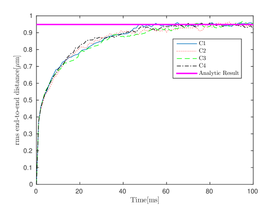
Fig. 2: The rms end-to-end distance for a compacted filament to re-extending towards the analytic (equilibrium) rms end-to-end distance in magenta for systems C1–C4 given in Table 3.

4 DNA binding model

To show the usefulness of the OMR model, we have devised an illustrative model for the relationship between a DNA binding protein and a segment of DNA. There is a large variety of different binding proteins, for example transcription factors or polymerases. In general, binding protein dynamics are not fully understood and vary greatly depending on the function of the protein [17]. In Brownian dynamics models, a binding protein binds to DNA with a given probability if it comes within a certain distance of the binding site on the DNA filament [10]. We will use a simple version of this approach and assume that a binding protein binds to DNA if it comes within a ‘binding radius’ of a bead in the bead-spring polymer chain.

We apply the multiscale aspect of the model by adjusting the resolution regime of the filament dynamically, so that as the binding protein moves close to the filament, nearby filament sections increase in resolution. To increase the resolution on-the-fly, we develop a Markov Chain Monte Carlo (MCMC) scheme. The model is presented as a two-resolution model for simplicity, but it can easily be extended to more resolution levels. We denote by $s$ the difference in resolution between high and low regions. Using the notation introduced in Definition 6, we consider filaments which include regions with higher resolution (where $s_{j}=1$ in Definition 6) and regions with lower resolution (where $s_{j}=s$).

4.1 Resolution increase with MCMC

We first present a framework for increasing the resolution between adjacent beads. If we wish to increase the resolution in a region of low resolution between beads $\mathbf{r}_{A}$ and $\mathbf{r}_{B}$ which lie a distance $d$ apart, then by Definition 6 we introduce $s^{2}-1$ new springs with Kuhn length $b$. We place the new beads between $\mathbf{r}_{A}$ and $\mathbf{r}_{B}$ to lie a distance of $d^{\prime}$ apart, which is in general not equal to $b$, because $d$ is in general not equal to $sb$. We select $d^{\prime}$ so that the rms end-to-end distance for the new chain formed is to equal $d$ at the time of its creation. Using equation (12), we require $d^{\prime}=d/s$ to be the distance between each bead. It should be noted that we are generating beads by the FJC model, introduced in Section 3.4.1 to be such that the distance between each new bead is the same. This is for simplicity as when we apply the dynamics there is a fast transition for these bond lengths to revert to the equilibrium distribution given by the Gaussian chain model [7].

In order to apply MCMC, we seek the probability function $\psi$ of a chain $F=\{\mathbf{r}_{i}\,|\,i=1,2,\ldots,M\}$ of $M=s^{2}-1$ beads a distance $d^{\prime}$ apart between $\mathbf{r}_{A}$ and $\mathbf{r}_{B}$. We first consider the probability function for the first $M-1$ beads $\{\mathbf{r}_{i<M}\}=\{\mathbf{r}_{i}\,|\,i=1,2,\ldots,M-1\}$, which is proportional to the circumference of the circle of points on which the last bead $\mathbf{r}_{M}$ can be placed, which we call the circle of allowable points $\Gamma$. This is given as the set

$$\Gamma=\{\mathbf{r}:|\mathbf{r}_{M-1}-\mathbf{r}|=d^{\prime}\ \text{and}\ |\mathbf{r}_{B}-\mathbf{r}|=d^{\prime}\},$$

or the set of all points a distance $d^{\prime}$ from both $\mathbf{r}_{M-1}$ and $\mathbf{r}_{B}$. In some cases $\Gamma=\emptyset$ when $|\mathbf{r}_{M-1}-\mathbf{r}_{B}|>2d^{\prime}$. Note that if $\psi(\{\mathbf{r}_{i<M}\})$ is proportional to the circumference of circle $\Gamma$ it is also proportional to its radius.

Provided $\Gamma\neq\emptyset$, to find the radius of $\Gamma$ we consider the triangle with points $\mathbf{r}_{M-1}$, $\mathbf{u}$ which is an arbitrary point on $\Gamma$, and $\mathbf{v}$ which is the midpoint between $\mathbf{r}_{M-1}$ and $\mathbf{r}_{B}$. By construction there is a right angle at $\mathbf{v}$. The radius of $\Gamma$ is given by the distance between $\mathbf{u}$ and $\mathbf{v}$, which is $l=\sqrt{d^{\prime 2}-(\lambda/2)^{2}},$ where $\lambda$ is the distance between $\mathbf{r}_{M-1}$ and $\mathbf{r}_{B}$. We therefore find the probability density function for the chain:

$$\psi(F)=\begin{cases}K\displaystyle\sqrt{d^{\prime 2}-(\lambda/2)^{2}}\prod_{i=1}^{M-1}\delta\Big{(}|\mathbf{r}_{i}-\mathbf{r}_{i-1}|-d^{\prime}\Big{)},&\mbox{if }\Gamma\neq\emptyset;\\ 0,&\mbox{if }\Gamma=\emptyset;\end{cases}$$

with normalisation constant $K$, $\mathbf{r}_{0}=\mathbf{r}_{A}$ and $\delta$ the Dirac delta function. To select from the probability distribution $\psi$, we apply the Metropolis-Hastings algorithm [4] as outlined in Algorithm 2.

Generate a proposal chain $\hat{F}=\{\mathbf{\hat{r}}_{i}\,|\,i=1,2,\ldots,M-1\}$ with each spring length $d^{\prime}$ starting at $\mathbf{r}_{A}$ from the FJC model.

if $|\mathbf{\hat{r}}_{M-1}-\mathbf{r}_{B}|<2d^{\prime}$ then

       Generate $\nu$ uniformly at random in $[0,1]$.

       Let $\alpha=\min(\psi(\hat{F})/\psi(F^{i}),1)$.

       if $\nu<\alpha$ then

             Pick $\mathbf{\hat{r}}_{M}$ uniformly at random on the circle of points distance $d^{\prime}$ from both $\mathbf{\hat{r}}_{M-1}$ and $\mathbf{r}_{B}$.

             Select $F^{i+1}=\hat{F}$.

      else

             Select $F^{i+1}=F^{i}$.

            

       end if

      

else

      Repeat and generate a new proposal chain.

end if

Algorithm 2 The algorithm for picking the next chain ${F}^{i+1}$ in the Metropolis-Hastings algorithm given the previous chain $F^{i}$.

Given the first $M-1$ beads, and provided $\Gamma\neq\emptyset$, the density function for the final bead is given by

$$\frac{1}{\sqrt{d^{\prime 2}-(\lambda/2)^{2}}}\,\delta(|\mathbf{r}_{M}-\mathbf{r}_{M-1}|-d^{\prime})\,\delta(|\mathbf{r}_{B}-\mathbf{r}_{M}|-d^{\prime}).$$

Algorithm 2 is a Metropolis-Hastings algorithm with a candidate-generating distribution which uses rejection sampling [31] to keep selecting chains $\hat{F}=\{\mathbf{\hat{r}}_{i}\,|\,i=1,2,\ldots,M-1\}$ with distance $d^{\prime}$ between each bead until we find a chain where the second last bead $\mathbf{\hat{r}}_{M-1}$ is within a distance $2d^{\prime}$ from the endpoint $\mathbf{r}_{B}$, which is then used as the candidate. Based on $10^{4}$ simulations we see approximately a $77.5\%$ acceptance of the candidate for $M\geq 3$ beads generated between beads a distance $b$ apart, invariant to the number of beads for $M\geq 3$. To ensure the Markov chain is sufficiently well mixed and that we have ‘lost memory’ of the initial chain, we choose the $10^{\text{th}}$ filament in the sequence generated from Algorithm 2; in $10^{3}$ simulations with a resolution difference of $3$, we see only one case where the initial distribution is the same as the $10^{\text{th}}$.

4.2 Model description

On top of our multiscale Rouse model, we introduce a binding protein, modelled as a diffusing particle with diffusion constant $D_{p}$. The position of the binding protein at time $t$ is denoted $\mathbf{p}(t)$. We assume that it evolves according to the discretized Brownian motion

$$\mathbf{p}(t+\Delta t)=\mathbf{p}(t)+\sqrt{2D_{p}\Delta t}\ \bm{\xi},$$ (20)

where $\bm{\xi}\sim[\mathcal{N}(0,1),\mathcal{N}(0,1),\mathcal{N}(0,1)]$ and $\Delta t$ is the time step of the highest resolution. Associated with the binding protein is a binding radius $d_{b}$, such that if any bead along the filament comes within a distance $d_{b}$ from the binding protein then it ‘binds’ to the filament and the simulation finishes. We also consider the protein to have drifted to infinity and fail to bind if it gets a distance $d_{\infty}$ from all beads which exist in the lowest resolution of the OMR model.

The binding protein also has its resolution increase radius $r_{I}$ (where $r_{I}>d_{b}$), so that if the protein is within a distance $r_{I}$ from a bead with an adjacent spring in low resolution then we change the spring to be high resolution and introduce new beads as described in Section 4.1, and reformulate bead radius, timestep and Kuhn length according to the OMR model in Definition 6. See Figure 3 for an example of the resolution increasing as the filament comes within range of the protein.

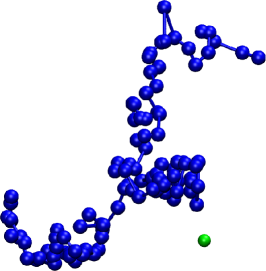
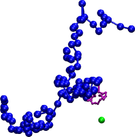
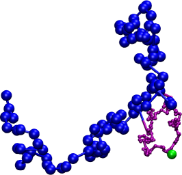
    (a)                                  (b)                                  (c)

Fig. 3: Snapshots of the DNA binding model, taken from an illustrative OMR simulation. In (a) the filament is represented by blue in its lowest resolution with the binding protein in green. This is a snapshot from just before the protein comes within resolution increase radius $r_{I}$. In (b) the protein has moved closer than this radius, so we increase the resolution in this region. The higher resolution region is shown in purple. We continue the simulation until either the protein drifts away from the filament or binds to it, as we see in (c).

As well as zooming in to specific areas of the filament, we include a provision that if the protein moves away far enough from the zoomed in filament section that it will not be interacting with the filament, then we zoom out. This is implemented as a zoom out factor $Z$, so that if the protein moves $Z\,r_{I}$ away from both beads on the boundary of a region in high resolution, then we ‘zoom out’ by changing the resolution of the region to the lower resolution and removing all beads inside.

To initialize the simulation, we generate the filament using the FJC model, with $R$ regions each containing one spring and the beads on the region boundaries denoted $\mathbf{q}_{j}(0)$, $j=1,2,\dots,R+1.$ Since all regions are in low resolution at time $t=0$, scalings (16) are given by

$$\widetilde{N}_{j}=1,\qquad\widetilde{b}_{j}=s\,b,\qquad\widetilde{\Delta t}_{j}=s^{4}\Delta t,\qquad\widetilde{\sigma}_{j}=s^{2}\sigma,$$ (21)

for all regions $j=1,2,\dots,R.$ We use $R=100$ in our illustrative simulations. We then place the protein uniformly at random on the sphere with radius $d_{0}$ centred at the middle bead of the chain (i.e. at the $(1+R/2)$-th bead). Once the initial configuration has been generated, we compute the time evolution of the filament and the protein iteratively using Algorithm 3, which describes one timestep of the method.

Calculate the position of the chain at time $t+\Delta t$ by Algorithm 1. Update both $\mathbf{r}_{n}(t+\Delta t)$ for $n=1,2,\dots,N(t)$ and $\mathbf{q}_{j}(t+\Delta t)$ for $j=1,2,\dots,R+1$.

Calculate the protein position at time $t+\Delta t$ by equation (20).

Set $t=t+\Delta t.$

if $\min_{1\leq n\leq N(t)}(|\mathbf{r}_{n}-\mathbf{p}|)<d_{b}$ then

       The protein binds to the filament. STOP the simulation.

      

else if $\min_{1\leq j\leq R+1}(|\mathbf{q}_{j}-\mathbf{p}|)>d_{\infty}$ then

       The protein drifts to infinity. STOP the simulation.

      

else

       for $\big{(}j=1,2,\dots,R\big{)}$ do

             if  (the $j$-th region is in the low resolution) then

                   if $\big{(}|\mathbf{q}_{j}-\mathbf{p}|<r_{I}$   OR   $|\mathbf{q}_{j+1}-\mathbf{p}|<r_{I}\big{)}$ then

                         Introduce new beads according to Algorithm 2.

                         Adjust bead radius, timestep and Kuhn length in the $j$-th region using Definition 6, i.e. use $\sigma$, $\Delta t$ and $b$, respectively.

                        

                   end if

                  

             else

                   (the $j$-th region is in the high resolution)

                   if $\big{(}|\mathbf{q}_{j}-\mathbf{p}|>Z\,r_{I}$   AND   $|\mathbf{q}_{j+1}-\mathbf{p}|>Z\,r_{I}\big{)}$ then

                         Remove all beads inside the $j$-th region.

                         Adjust bead radii $\widetilde{\sigma}_{j}$, timestep $\widetilde{\Delta t}_{j}$ and Kuhn length $\widetilde{b}_{j}$ in the $j$-th region by (21).

                        

                   end if

                  

             end if

            

       end for

      

end if

Algorithm 3 One iteration of the algorithm for the DNA binding model.

At each time step, the multi-resolution bead-spring polymer is described as in Definition 1 by the positions of $N\equiv N(t)$ beads at $\mathbf{r}_{n}\equiv\mathbf{r}_{n}(t)=[r_{n,1}(t),r_{n,2}(t),r_{n,3}(t)]$, $n=1,2,\dots,N(t).$ We initially have $N(0)=R+1$ beads at positions $\mathbf{r}_{n}(0)=\mathbf{q}_{n}(0)$, for $n=1,2,\dots,N(0).$ As time progresses, some regions are refined, so the value of $N(t)$ changes and indices of some beads are relabelled. To simplify the presentation of Algorithm 3, we denote by $\mathbf{q}_{j}\equiv\mathbf{q}_{j}(t)$, $j=1,2,\dots,R+1,$ the positions of boundary beads of each region at time $t$, independently of the fact whether the chain was refined or not in the corresponding region.

We have confirmed the consistency of the model where resolutions are changed dynamically against analytic results. It performs well with a rms end-to-end distance of $2.997\,\mu\rm{m}$ and diffusion of $7.49\cdot 10^{-5}\,\mu\rm{m^{2}s^{-1}}$ compared to expected results from (9) and (14) of $3\,\mu\rm{m}$ and $7.34\cdot 10^{-5}\,\mu\rm{m^{2}s^{-1}}$, respectively, after $10^{3}$ simulations, with parameters given in (19) and Table 4.

4.3 Results

We compare the results between the OMR model with the classical Rouse model, with the entire filament in the highest resolution. We run Algorithm 3 with the parameters given in (19) and Table 4.

​​Symbol​​	Name	Value	Justification
$r_{I}$	Resolution increase radius	$0.5\,\mu\rm{m}$	Chosen to ensure no instant binding of protein to filament after resolution increase
$s$	Resolution difference	$3$	Arbitrary
$D_{p}$	Protein diffusion constant parameter	$$2\text{\times}{10}^{-5}$\mu\rm{m^{2}s^{-1}}$	Approx. the diffusion constant for the filament
$d_{b}$	Binding radius	$0.01\,\mu\rm{m}$	Arbitrary
$d_{\infty}$	Drift to infinity distance	$1\,\mu\rm{m}$	Arbitrary
$Z$	Zoom factor	$5$	Arbitrary
$R$	Number of regions	$100$	Initial number of beads

Table 4: Parameter selection for the DNA binding model, with the remaining parameters identical to those given in (19).

At different initial starting distances the model runs until the protein is either bound or has escaped the filament. In Figure 4, we present the probability of binding of the protein to the filament, $P_{b}(d_{0})$, as a function of the initial distance $d_{0}\in[d_{b},10\,d_{\infty}]$ of the protein from the middle bead of the filament. We estimate $P_{b}(d_{0})$ as a fraction of simulations which end up with the protein bound to DNA. Each data point in Figure 4 represents the value of $P_{b}(d_{0})$ estimated from $10^{3}$ independent realizations of the process. If $d_{0}<d_{b}$, then the protein is immediately bound to DNA, i.e. $P_{b}(d_{0})=1$ for $d_{0}<d_{b}$. If $d_{0}=d_{\infty}$, then the probability of binding is nonzero, because the initial placement, $d_{0}$, is the distance of the protein from the centre of the filament. In particular, the minimum distance from protein to filament is less than or equal to the initial placement distance, $d_{0}$, and the simulations (with the possibility of binding) take place even if $d_{0}=d_{\infty}$.

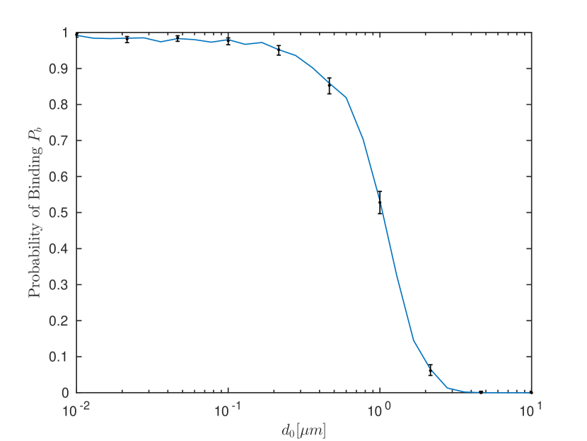
Fig. 4: A comparison between the probability of binding of the protein to the DNA filament, $P_{b}(d_{0})$, depending on starting distance, $d_{0}$, from the filament for the single-scale (black points) and OMR (blue line) models. Error bars give a 95% confidence interval based on the Wilson score interval for binomial distributions [44].

Due to computational constraints of the single-scale model we consider a selection of initial distances at points $d_{0}=10^{-2+\ell/3}\,\mu$m, $\ell=0,1,\dots,9$ (black points), where error bars give a 95% confidence interval based on the Wilson score interval for binomial distributions [44]. We run simulations for more initial distances, $d_{0}=10^{-2+\ell/9}\,\mu$m, $\ell=0,1,\dots,27$ (blue line), using the computationally efficient OMR model and present our results as the blue line in Figure 4. We see that $P_{b}(d_{0})$ is very similar between the single-scale and OMR models. The model also succeeds in reducing computational time. For $10^{3}$ simulations with the protein starting $1\,\mu\rm{m}$ from the middle bead, with parameters given in Table 4, the OMR model represented a 3.2-times speedup compared to the detailed model, with only a 3-times resolution difference. We expect for larger resolution differences to see greater improvements in speed.

5 Discussion

In this paper we have extended basic filament modelling techniques to multiple scales by developing OMR methods. We have presented an MCMC approach for increasing the resolution along a static filament segment, as well as an extension to the Rouse model to dynamically model a filament which considers multiple scales. The bead radius, as well as the number of beads associated with each resolution, is altered to maintain consistency with the end-to-end distance and diffusion of a filament across multiple scales, as well as the timestep to ensure numerical convergence.

We have then illustrated the OMR methodology using a simple model of protein binding to a DNA filament, in which the OMR model gave similar results to the single-scale model. We have also observed a 3.2-times speed-up in computational time on a model which considers only a 3-times increase in resolution, which illustrates the use of the OMR approach as a method to speed up simulations whilst maintaining the same degree of accuracy as the more computationally intensive single-scale model. The speed-up in computational time could be further increased by replacing Brownian dynamics based on time-discretization (20) by event-based algorithms such as the FPKMC (First passage kinetic Monte Carlo) and GFRD (Green’s function reaction dynamics) methods [33, 43].

When considering the zooming out of the DNA binding model, note that it is generally possible to zoom in and out repetitively, as long as the dynamics are such that we can generate a high resolution structure independent from the previous one (i.e., once we zoom out, the microscopic structure is completely forgotten). However, particularly in the case of chromatin, histone modification and some DNA-binding proteins may act as long-term memory at a microscopic scale below the scales currently considered. To reflect the effect of the memory, some properties of the microscopic structure should be maintained even after zooming out. Fractal dimension may serve as a candidate of indices [29], which can be also estimated in living cells by single-molecule tracking experiments [41].

The OMR method could be applied to modern simulations of DNA and other biological polymers which use the Rouse model [19] in situations where certain regions of the polymer require higher resolutions than other regions. The model considered in this report uses Rouse dynamics, which is moderately accurate given its simplicity, but as we zoom in further towards a binding site, then we will need to start to consider hydrodynamic forces and excluded volume effects acting between beads. Models which include hydrodynamic interactions such as the Zimm model [47] have previously been used to look at filament dynamics [1, 11]. Therefore it is of interest to have a hybrid model which uses the Rouse model in low resolutions and the Zimm model in high resolutions. The combination of different dynamical models might give interesting results regarding hierarchical structures forming as we move between resolutions.

As we go into higher resolutions, strands of DNA can be modelled as smooth [2], unlike the FJC model where angles between beads are unconstrained. The wormlike chain model of Kratky and Porod [23], implemented via algorithm by Hagermann and Zimm [15], gives a non-uniform probability distribution for the angles between each bead. Allison [1] then implements the Zimm model dynamics on top of the static formulation to give bending as well as stretching forces. Another interesting open multiscale problem is to implement this at higher resolutions, with the Rouse model at lower resolutions, in order to design a hybrid model.

To introduce even more realism, we would see individual histones and consider forces between these as in the model of Rosa and Everaers [35] which includes Lennard-Jones and FENE forces between beads. As we approach an atomistic level, it may be interesting to consider a molecular dynamics approach to modelling the DNA filament. Coarser Brownian dynamics models can be estimated from molecular dynamics models either analytically [8] or numerically [9], depending on the complexity of the molecular dynamics model. A variety of structure-based coarse-grained models have been used for chromatin (e.g. [30]), also with transcription factors [42]. Multiscale modelling techniques (e.g. [22] with iterative coarse-graining), as well as adaptive resolution models (e.g. [46] for solvent molecules), have been developed. We expect these studies will connect with polymer-like models at a certain appropriate length and time scale. On top of this, models for the target searching process by proteins such as transcription factors could be improved (for example, by incorporating facilitated diffusion under crowded environment [3]).

The need for developing and analyzing multiscale models of DNA which use one of the above detailed simulation approaches for small parts of the DNA filament is further stimulated by recent experimental results. Chromosome conformation capture (3C)-related techniques, particularly at a genome-wide level using high-throughput sequencing (Hi-C [26]), provide the three-dimensional structure of the chromosomes in an averaged manner. Moreover, recent imaging techniques have enabled us to observe simultaneously the motion and transcription of designated gene loci in living cells [32]. Simulated processes could be compared with such experimental results. Recent Hi-C experiments also revealed fine structures such as loops induced by DNA-binding proteins [39]. To develop more realistic models, information about the binding sites for these proteins may be utilized when we increase the resolution in our scheme.

References

- [1] S. A. Allison. Brownian dynamics simulation of wormlike chains. Fluorescence depolarization and depolarized light scattering. Macromolecules, 19:118–124, 1986.
- [2] S. S. Andrews. Methods for modeling cytoskeletal and DNA filaments. Phys. Biol., 11:011001, 2014.
- [3] C. A. Brackley, M. E. Cates, and D. Marenduzzo. Intracellular facilitated diffusion: searchers, crowders, and blockers. Phys. Rev. Lett., 111(10):108101, 2013.
- [4] S. Chib and E. Greenberg. Understanding the Metropolis-Hastings algorithm. Amer. Statist., 49:327–335, 1995.
- [5] T. Cremer, M. Cremer, B. Hübner, et al. The 4D nucleome: Evidence for a dynamic nuclear landscape based on co-aligned active and inactive nuclear compartments. FEBS Lett., 589(20A):2931–2943, 2015.
- [6] P. De Gennes. Scaling concepts in polymer physics. Cornell university press, 1979.
- [7] M. Doi and S. F. Edwards. The theory of polymer dynamics. Oxford University Press, 1988.
- [8] R. Erban. From molecular dynamics to Brownian dynamics. Proceedings of the Royal Society A, 470:20140036, 2014.
- [9] R. Erban. Coupling all-atom molecular dynamics simulations of ions in water with Brownian dynamics. Proceedings of the Royal Society A 472:20150556, 2016.
- [10] R. Erban and S. J. Chapman. Stochastic modelling of reaction–diffusion processes: algorithms for bimolecular reactions. Physical Biology, 6:046001, 2009.
- [11] D. L. Ermak and J. A. McCammon. Brownian dynamics with hydrodynamic interactions. J. Chem. Phys., 69:1352–1360, 1978.
- [12] G. Felsenfeld and M. Groudine. Controlling the double helix. Nature, 421:448–453, 2003.
- [13] M. B. Flegg, S. J. Chapman, and R. Erban. The two-regime method for optimizing stochastic reaction-diffusion simulations. J. R. Soc. Interface, 9:859–868, 2012.
- [14] E. Guth and H. Mark. Zur innermolekularen, Statistik, insbesondere bei Kettenmolekiilen I. Monatsh. Chem., 65:93–121, 1934.
- [15] P. J. Hagerman and B. H. Zimm. Monte Carlo approach to the analysis of the rotational diffusion of wormlike chains. Biopolymers, 20:1481–1502, 1981.
- [16] P. J. Hagerman. Flexibility of DNA. Annu. Rev. Biophys. Bio., 17(1), 1988.
- [17] S. E. Halford, and J. F. Marko. How do site-specific DNA-binding proteins find their targets? Nucleic Acids Res., 32(10), 2004.
- [18] A. Hotz, and R. E. Skelton. Covariance control theory. Int. J. Control, 46(1), 1987.
- [19] J. S. Hur, E.S. Shaqfeh, and R. G. Larson. Brownian dynamics simulations of single DNA molecules in shear flow. Journal of Rheology, 44(4):713–742, 2000.
- [20] P. Kloeden and E. Platen. Numerical Solution of Stochastic Differential Equations. Springer, Berlin.
- [21] R. D. Kornberg. Chromatin structure: a repeating unit of histones and DNA. Science, 184:868–871, 1974.
- [22] N. Korolev, L. Nordenskiöld, and A. P. Lyubartsev. Multiscale coarse-grained modelling of chromatin components: DNA and the nucleosome. Adv. Colloid Interface Sci., 232:36–48, 2016.
- [23] O. Kratky and G. Porod. Röntgenuntersuchung gelöster Fadenmoleküle. Recl. Trav. Chim. Pay. B., 68:1106–1122, 1949.
- [24] K. Kremer and G. S. Grest. Dynamics of entangled linear polymer melts: A molecular-dynamics simulation. J. Chem. Phys., 92:5057–5086, 1990.
- [25] W. Kuhn. Über die Gestalt fadenförmiger Moleküle in lösungen. Colloid. Polym. Sci., 68:2–15, 1934.
- [26] E. Lieberman-Aiden, N. L. van Berkum, et al. Comprehensive mapping of long-range interactions reveals folding principles of the human genome. Science, 326(5950):289–293, 2009.
- [27] K. Maeshima, K. Kaizu, S. Tamura, T. Nozaki, T. Kokubo, and K. Takahashi. The physical size of transcription factors is key to transcriptional regulation in chromatin domains. J. Phys-Condens. Mat., 27:064116, 2015.
- [28] K. Maeshima, R. Rogge, et al. Nucleosomal arrays self-assemble into supramolecular globular structures lacking 30-nm fibers. EMBO J., 35(10):1115–1132, 2016.
- [29] L. A. Mirny. The fractal globule as a model of chromatin architecture in the cell. Chromosome Res. 19:37–51, 2011.
- [30] O. Müller, N. Kepper, R. Schöpflin, R. Ettig, K. Rippe, and G. Wedemann. Changing chromatin fiber conformation by nucleosome repositioning. Biophys. J., 107(9):2141–2150, 2014.
- [31] R. M. Neal. Slice sampling. Ann. Statist., 31:705–767, 2003.
- [32] H. Ochiai, T. Sugawara, and T. Yamamoto. Simultaneous live imaging of the transcription and nuclear position of specific genes. Nucl. Acids Res., 43(19):e127, 2015.
- [33] T. Opplestrup, V. Bulatov, A. Donev, et al. First-passage kinetic Monte Carlo method. Physical Review E, 80(6):066701, 2009.
- [34] D. Richter, A. Baumgärtner, K. Binder, B. Ewen, and J. B. Hayter. Dynamics of collective fluctuations and Brownian motion in polymer melts. Phys. Rev. Lett., 47:109–113, Jul 1981.
- [35] A. Rosa and R. Everaers. Structure and dynamics of interphase chromosomes. PLoS Comput. Biol., 4:e1000153, 2008.
- [36] R. Robertson, S. Laib and D. Smith. Diffusion of isolated DNA molecules: Dependence on length and topology. Proc. Natl. Acad. Sci. USA, 103(19):7310-7314, 2006.
- [37] J. Rotne and S. Prager. Variational treatment of hydrodynamic interaction in polymers. J. Chem. Phys., 50:4831–4837, 1969.
- [38] P. E. Rouse. A theory of the linear viscoelastic properties of dilute solutions of coiling polymers. J. Chem. Phys., 21:1272–1280, 1953.
- [39] A. L. Sanborn, S. S. P. Rao, S. Huang, et al. Chromatin extrusion explains key features of loop and domain formation in wild-type and engineered genomes. Proc. Natl. Acad. Sci. USA, 112(47):E6456–E6465, 2015.
- [40] Y. Saito and M. Mitsui. Stability analysis of numerical schemes for stochastic differential equations. SIAM J. Numer. Anal., 33:2254–2267, 1996.
- [41] S. Shinkai, T. Nozaki, K. Maeshima, and Y. Togashi. Dynamic nucleosome movement provides structural information of topological chromatin domains in living human cells. bioRxiv doi:10.1101/059147, 2016.
- [42] S. Takada, R. Kanada, C. Tan, T. Terakawa, W. Li, and H. Kenzaki. Modeling structural dynamics of biomolecular complexes by coarse-grained molecular simulations. Acc. Chem. Res., 48(12):3026–3035, 2015.
- [43] K. Takahashi, S. Tanase-Nicola and P. ten Wolde. Spatio-temporal correlations can drastically change the response of a MAPK pathway. Proc. Natl. Acad. Sci. USA, 107:19820-19825, 2010.
- [44] E. B. Wilson. Probable inference, the law of succession, and statistical inference J. Amer. Statist. Assoc., 22(158):209–212, 1927.
- [45] A. Wolffe. Chromatin. Academic Press, third edition, 2000.
- [46] J. Zavadlav, R. Podgornik, and M. Praprotnik. Adaptive resolution simulation of a DNA molecule in salt solution. J. Chem. Theory Comput., 11(10):5035–5044, 2015.
- [47] B. H. Zimm. Dynamics of polymer molecules in dilute solution: Viscoelasticity, flow birefringence and dielectric loss. J. Chem. Phys., 24(2):269–278, 1956.