Diffuse interface approaches in atmosphere and ocean - modeling and numerical implementation

Abstract

We propose to model physical effects at the sharp density interface between atmosphere and ocean with the help of diffuse interface approaches for multiphase flows with variable densities. We use the variable-density model proposed in m6:AbelsGarckeGruen_CHNSmodell . This results in a Cahn-Hilliard/Navier-Stokes type system which we complement with tangential Dirichlet boundary conditions to incorporate the effect of wind in the atmosphere. Wind is responsible for waves at the surface of the ocean, whose dynamics have an important impact on the $CO_{2}-$exchange between ocean and atmosphere. We tackle this mathematical model numerically with fully adaptive and integrated numerical schemes tailored to the simulation of variable density multiphase flows governed by diffuse interface models. Here, fully adaptive, integrated, efficient, and reliable means that the mesh resolution is chosen by the numerical algorithm according to a prescribed error tolerance in the a posteriori error control on the basis of residual-based error indicators, which allow to estimate the true error from below (efficient) and from above (reliable). Our approach is based on the work of m6:HintermuellerHinzeKahle_adaptiveCHNS ; m6:GarckeHinzeKahle_CHNS_AGG_linearStableTimeDisc , where a fully adaptive efficient and reliable numerical method for the simulation of two-dimensional multiphase flows with variable densities is developed. We incorporate the stimulation of surface waves via appropriate boundary conditions.

1 Introduction

The energy and momentum transfer from the atmosphere to the ocean is an essential ingredient for the accurate modelling of the energy cycle. In fact, the vast majority of the energy input to the ocean comes from the winds ($\sim$20 TW), with much smaller inputs from tides ($\sim$3.5 TW) and geothermal heating ($\sim$0.05 TW) (m6:wunsch2004, , numbers taken from). It is therefore not surprising that the energy transfer from the wind to the surface wave field, and the ensuing energy dissipation through breaking waves, represents the largest transfer of energy in the oceans m6:wunsch2004 . Despite the enormous importance of the processes of surface wave generation and dissipation, there are still fundamental gaps in our ability to conduct both process modelling, and observational studies of these processes operating near the air-sea interface.

However, many major advances have recently been made through the use of powerful numerical simulations (m6:sullivan2010, , see the recent review by). These simulations have shown that classical modelling and parameterisation techniques, such as the use of the law-of-the-wall turbulence scaling, must be revised to account for the dynamics of wind waves. Here we outline a number of these results that must be included if an accurate, and energy consistent, treatment of atmosphere-ocean interactions is to be accomplished.

The transport of momentum from the atmosphere to the ocean in all but the finest scale modelling is largely done through specification of a bulk drag coefficient. This coefficient attempts to capture the complex fluid flows around the air-water interface, as well as the dissipation processes therein. This momentum (and energy) flux must then be partitioned between a number of different processes such as wind-wave growth, turbulent kinetic energy and dissipation through wave breaking, and the generation of wave-induced currents such as Langmuir circulations and Stokes drift. All of these processes have been found to be important for the distribution of turbulent kinetic energy and dissipation in the surface mixed layer of the ocean m6:sullivan2007 . Wave breaking has been found to lead to turbulence levels that are two orders of magnitude larger at the near-surface than the often used law-of-the-wall scaling predicts m6:drennan1996 ; m6:sutherland2015 . Breaking is also responsible for generating large increases in the mean flow (Stokes drift) of the wave-affected near surface layer, which then provides a mechanism for the development of strong Langmuir circulations within the surface mixed layer m6:mcwilliams1997 . These Langmuir circulations have been found to then redistribute the high turbulent kinetic energy throughout the surface mixed layer of the ocean m6:sullivan2007 . Not only are the Langmuir circulations responsible for the redistribution of turbulent kinetic energy in the mixed layer, but this process is also found to contribute to the generation of internal waves at the base of the mixed layer that transport energy into the deeper ocean m6:polton2008 .

We propose to use the thermodynamically consistent diffuse interface model proposed in m6:AbelsGarckeGruen_CHNSmodell to model the air-water interface between atmosphere and ocean. This model will be extended to produce a series of direct numerical simulations of wind generated waves. Only very few studies have examined the evolution of wind-waves using such a fundamental approach m6:kihara2007 ; m6:shen2003 ; m6:sullivan2000 ; m6:sullivan2002 ; m6:tsai2007 ; m6:tsai2015 ; m6:lubin2015 . However, these studies often do not involve a proper coupling of the water surface and the air flow above. For example, the water surface is often replaced by another simpler boundary condition, such as an impermeable sinusoidal wall m6:shen2003 , or an uncoupled propagating water wave solution m6:sullivan2000 ; m6:sullivan2002 . The recent study of m6:lubin2015 has shown how powerful a direct coupling of the air and water layers is for predicting turbulent air-entraining structures in the breaking of surface waves. Another study that utilises a fully coupled treatment of the air and water layers is that of m6:tsai2015 . They show the important result that turbulent water flows are generated even under the conditions of non-breaking surface waves. We believe that the diffuse interface methods developed for the Cahn-Hilliard/Navier-Stokes system will provide an improved method to deal with the current short comings of simulating a direct coupling of the air-water interface. We recall here that one reason is its flexibility in the numerical treatment of topology changes, which might occur in e.g. breaking waves, and another reason is the mass-conserving property of the approach, see e.g. m6:HintermuellerHinzeKahle_adaptiveCHNS . On the long run it is planed to use the method to simulate wind-wave growth and be compare the numerical results to laboratory experiments using the PIV technique to resolve the airflow and water surface elevation.

The diffuse interface method of treating the air-water interface using the Cahn-Hilliard/Navier-Stokes (CHNS) system forms a new approach to the model studies described so far. We note, however, that there are several contributions to numerical approaches to the simulation of multiphase flows in the sharp interface formulation. Here we refer, e.g., to the book of m6:GrossReusken_NumMethTwoPhaseFlow , the work of m6:GanesanTobiska09 as well as the works of m6:BGN14 ; m6:TurekWan07 . A benchmark for sharp interface approaches to the numerical simulation of rising bubble dynamics is proposed by m6:Hysing_Turek_quantitative_benchmark_computations_of_two_dimensional_bubble_dynamics , which is accomplished with diffuse interface simulations by m6:Aland_Voigt_bubble_benchmark . A review of the development of phase-field models and their numerical methods for multi-component fluid flows with interfacial phenomena is given by m6:Kim12 . In the context of mechanical engineering and meteorological applications phase-field models for two-phase flows are often referred to as the two-fluid formulation, see e.g. m6:MSSP10 , and m6:DE98 , compare also the related volume-of-fluid schemes, see e.g. m6:Lowengrub04 , as well as the references cited therein.

Since the dynamics of multiphase flows essentially depend on the dynamics at the interfaces it is important to resolve the interfacial region in diffuse interface models well. Here, adaptive numerical concepts are the method of choice. Concerning the existing literature on the solver development for the coupled CHNS system we note that in m6:KayWelford_efficientsolution a robust (with respect to the interfacial width) nonlinear multigrid method was introduced with a double-well homogeneous free energy density. We refer to m6:KayWelford_multigridsolver for the multigrid solver for the Cahn-Hilliard (CH) part only. Later, in m6:KayStylesWelford error estimates for the coupled system were derived and numerically verified. Coupled CHNS systems were also considered in m6:BoyerLapuerteMinjeaud with a double-well potential in the case of three-phase flows; see also m6:Boyer_shear ; m6:Boyer_two_phase_different_densities ; m6:BoyerChupinFabrie and m6:AlandVoigt10 ; m6:Aland_Voigt_bubble_benchmark as well as the references therein for rather qualitative studies of the behaviour of multiphase and mixture flows.

Stable numerical schemes for the recently developed thermodynamically consistent diffuse interface model m6:AbelsGarckeGruen_CHNSmodell are developed in m6:GarckeHinzeKahle_CHNS_AGG_linearStableTimeDisc ; m6:GruenMetzger__CHNS_decoupled ; m6:Gruen_Klingbeil_CHNS_AGG_numeric . Concerning the numerical treatment of the sole CH system many contributions can be found in the literature. For a rather comprehensive discussion of available solvers we refer to m6:HintermuellerHinzeTber . In the latter work, a fully integrated adaptive finite element approach for the numerical treatment of the CH system with a non-smooth homogeneous free energy density was developed. The notion of a fully adaptive method relates to the fact that the local mesh adaptation is based on rigorous residual based a posteriori error estimates (rather than heuristic techniques based on, e.g., thresholding the discrete concentration or the discrete concentration gradient). The concept of an integrated adaptation couples the adaptive cycle and the underlying solver as the latter might need to be equipped with additional stabilisation methodologies such as the Moreau-Yosida regularisation in the case of non-smooth homogeneous free energy densities for guaranteeing mesh independence. The latter is indeed obtained upon balancing regularisation and discretisation errors. When equipped with a multi-grid scheme for solving the linear systems occurring in the underlying semi-smooth Newton iteration, an overall iterative scheme is obtained which is optimal in the sense that the computational effort grows only linearly in the number of degrees of freedom.

In m6:HintermuellerHinzeKahle_adaptiveCHNS the approach of m6:HintermuellerHinzeTber is extended to a fully practical adaptive solver for the two-dimensional CHNS system with a double obstacle potential according to m6:BloweyElliott_I . To the best of the applicants knowledge the work of m6:HintermuellerHinzeKahle_adaptiveCHNS contains the first rigorous approach to reliable and efficient residual based a posteriori error analysis for multi phase flows governed by diffuse interface models. This approach is combined with a stable, energy conserving time integration scheme in m6:GarckeHinzeKahle_CHNS_AGG_linearStableTimeDisc to a fully reliable and efficient adaptive and energy conserving a posteriori concept for the numerical treatment of variable density multiphase flows. This approach was very successfully validated against the existing sharp and diffuse interface rising benchmarks of m6:Hysing_Turek_quantitative_benchmark_computations_of_two_dimensional_bubble_dynamics and m6:Aland_Voigt_bubble_benchmark , respectively in the field.

2 Diffuse interface approach

2.1 Notation

Let $\Omega\subset\mathbb{R}^{n}$, $n\in\{2,3\}$ denote a bounded domain with boundary $\partial\Omega$ and unit outer normal $\nu_{\Omega}$. Let $I=(0,T]$ denote a time interval.

We use the conventional notation for Sobolev and Hilbert Spaces, see e.g. m6:Adams_SobolevSpaces . With $L^{p}(\Omega)$, $1\leq p\leq\infty$, we denote the space of measurable functions on $\Omega$, whose modulus to the power $p$ is Lebesgue-integrable. $L^{\infty}(\Omega)$ denotes the space of measurable functions on $\Omega$, which are essentially bounded. For $p=2$ we denote by $L^{2}(\Omega)$ the space of square integrable functions on $\Omega$ with inner product $(\cdot,\cdot)$ and norm $\|\cdot\|$. For a subset $D\subset\Omega$ and functions $f,g\in L^{2}(\Omega)$ we by $(f,g)_{D}$ denote the inner product of $f$ and $g$ restricted to $D$, and by $\|f\|_{D}$ the respective norm. By $W^{k,p}(\Omega)$, $k\geq 1,1\leq p\leq\infty$, we denote the Sobolev space of functions admitting weak derivatives up to order $k$ in $L^{p}(\Omega)$. If $p=2$ we write $H^{k}(\Omega)$. The subset $H^{1}_{0}(\Omega)$ denotes $H^{1}(\Omega)$ functions with vanishing boundary trace.
We further set

$$L^{2}_{(0)}(\Omega)=\{v\in L^{2}(\Omega)\,|\,(v,1)=0\},$$

and with

$$H(\mbox{div},\Omega)=\{v\in H^{1}_{0}(\Omega)^{n}\,|\,(\mbox{div}(v),q)=0\,\forall q\in L^{2}_{(0)}(\Omega)\}$$

we denote the space of all weakly solenoidal $H^{1}_{0}(\Omega)$ vector fields.
For $u\in L^{q}(\Omega)^{n}$, $q>n$, and $v,w\in H^{1}(\Omega)^{n}$ we introduce the trilinear form

$$a(u,v,w)=\frac{1}{2}\int_{\Omega}\left(\left(u\cdot\nabla\right)v\right)w\,dx-\frac{1}{2}\int_{\Omega}\left(\left(u\cdot\nabla\right)w\right)v\,dx.$$

Note that there holds $a(u,v,w)=-a(u,w,v)$, and especially $a(u,v,v)=0$.

2.2 The mathematical model

In the present work we consider the following diffuse interface model for two-phase flows with variable densities proposed in m6:AbelsGarckeGruen_CHNSmodell :

$$\rho\partial_{t}v+\left(\left(\rho v+J\right)\cdot\nabla\right)v-\mbox{div}\left(2\eta Dv\right)+\nabla p= \mu\nabla\varphi+\rho g \forall x\in\Omega,\,\forall t\in I,$$ (1)

$$\mbox{div}(v)= 0 \forall x\in\Omega,\,\forall t\in I,$$ (2)

$$\partial_{t}\varphi+v\cdot\nabla\varphi-\mbox{div}(m\nabla\mu)= 0 \forall x\in\Omega,\,\forall t\in I,$$ (3)

$$-\sigma\epsilon\Delta\varphi+\frac{\sigma}{\epsilon}F^{\prime}(\varphi)-\mu= 0 \forall x\in\Omega,\,\forall t\in I,$$ (4)

$$v(0,x)= v_{0}(x) \forall x\in\Omega,$$ (5)

$$\varphi(0,x)= \varphi_{0}(x) \forall x\in\Omega,$$ (6)

$$v(t,x)= 0 \forall x\in\partial\Omega,\,\forall t\in I,$$ (7)

$$\nabla\mu(t,x)\cdot\nu_{\Omega}=\nabla\varphi(t,x)\cdot\nu_{\Omega}= 0 \forall x\in\partial\Omega,\,\forall t\in I,$$ (8)

where $J=-\frac{d\rho}{d\varphi}m\nabla\mu$. Here $\Omega\subset\mathbb{R}^{n},\,n\in\{2,3\}$, denotes an open and bounded domain, $I=(0,T]$ with $0<T<\infty$ a time interval, $\varphi$ denotes the phase field, $\mu$ the chemical potential, $v$ the volume averaged velocity, $p$ the pressure, and $\rho=\rho(\varphi)=\frac{1}{2}\left((\rho_{2}-\rho_{1})\varphi+(\rho_{1}+\rho_{2})\right)$ the mean density, where $0<\rho_{1}\leq\rho_{2}$ denote the densities of the involved fluids. The viscosity is denoted by $\eta$ and can be chosen as an arbitrary positive function fulfilling $\eta(-1)=\tilde{\eta}_{1}$ and $\eta(1)=\tilde{\eta}_{2}$, with individual fluid viscosities $\eta_{1},\eta_{2}$. The mobility is denoted by $m=m(\varphi)$. The gravitational force is denoted by $g$. By $Dv=\frac{1}{2}\left(\nabla v+(\nabla v)^{t}\right)$ we denote the symmetrized gradient. The scaled surface tension is denoted by $\sigma$ and the interfacial width is proportional to $\epsilon$. The free energy is denoted by $F$. For $F$ we use a splitting $F=F_{+}+F_{-}$, where $F_{+}$ is convex and $F_{-}$ is concave.

The above model couples the Navier–Stokes equations (1)–(2) to the Cahn–Hilliard model (3)–(4) in a thermodynamically consistent way, i.e. a free energy inequality holds. It is the main goal to introduce and analyze an (essentially) linear time discretization scheme for the numerical treatment of (1)–(8), which also on the discrete level fulfills the free energy inequality. This in conclusion leads to a stable scheme that is thermodynamically consistent on the discrete level.

Existence of weak solutions to system (1)–(8) for a specific class of free energies $F$ is shown in m6:AbelsDepnerGarcke_CHNS_AGG_exSol ; m6:AbelsDepnerGarcke_CHNS_AGG_exSol_degMob . See also the work m6:Gruen_convergence_stable_scheme_CHNS_AGG , where the existence of weak solutions for a different class of free energies $F$ is shown by passing to the limit in a numerical scheme. We refer to m6:AkiDreyer_QuasiIncompressibleInterfaceModel , m6:Boyer_two_phase_different_densities , m6:Ding_Spelt_Shu_diffuse_interface_model_diff_density , m6:Lowengrub_CahnHilliard_and_Topology_transitions , and the review m6:AndersenFaddenWheeler for other diffuse interface models for two-phase incompressible flow. Numerical approaches for different variants of the Navier–Stokes Cahn–Hilliard system have been studied in m6:Aland_Voigt_bubble_benchmark , m6:Boyer_two_phase_different_densities , m6:Feng_FullyDiscreteNSCH , m6:Gruen_convergence_stable_scheme_CHNS_AGG , m6:Gruen_Klingbeil_CHNS_AGG_numeric , m6:GuoLinLowengrub_numericalMethodForCHNS_Lowengrub , m6:HintermuellerHinzeKahle_adaptiveCHNS , m6:HintermuellerHinzeKahle_adaptiveCHNS , m6:GruenMetzger__CHNS_decoupled , and m6:KayStylesWelford .

Our numerical treatment approach is based on the following weak formulation, which is proposed in m6:GarckeHinzeKahle_CHNS_AGG_linearStableTimeDisc .

Definition 1

We call $v$, $\varphi$, $\mu$ a weak solution to (1)–(8) if $v(0)=v_{0}$, $\varphi(0)=\varphi_{0}$, $v(t)\in H(\mbox{div},\Omega)$ for $a.e.\,t\in I$ and

$$\frac{1}{2}\int_{\Omega}\left(\partial_{t}(\rho v)+\rho\partial_{t}v\right)w\,dx+\int_{\Omega}2\eta Dv:Dw\,dx$$

$$+a(\rho v+J,v,w)=\int_{\Omega}\mu\nabla\varphi w+\rho gw\,dx \quad\forall w\in H(\mbox{div},\Omega),$$ (9)

$$\int_{\Omega}\left(\partial_{t}\varphi+v\cdot\nabla\varphi\right)\Phi\,dx+\int_{\Omega}m(\varphi)\nabla\mu\cdot\nabla\Phi\,dx=0 \quad\forall\Phi\in H^{1}(\Omega),$$ (10)

$$\sigma\epsilon\int_{\Omega}\nabla\varphi\cdot\nabla\Psi\,dx+\frac{\sigma}{\epsilon}\int_{\Omega}F^{\prime}(\varphi)\Psi\,dx-\int_{\Omega}\mu\Psi\,dx=0 \quad\forall\Psi\in H^{1}(\Omega),$$ (11)

is satisfied for almost all $t\in I$.

For the assumptions on the data we refer to m6:GarckeHinzeKahle_CHNS_AGG_linearStableTimeDisc . In the present work we use the relaxed double-obstacle free energy given by

$$F(\varphi) =\frac{1}{2}\left(1-\varphi^{2}+s\lambda^{2}(\varphi)\right),$$ (12)

with

$$\lambda(\varphi) :=\max(0,\varphi-1)+\min(0,\varphi+1),$$

where $s\gg 0$ denotes the relaxation parameter. $F$ is introduced in m6:HintermuellerHinzeTber as Moreau–Yosida relaxation of the double-obstacle free energy

$$F^{obst}(\varphi)=\begin{cases}\frac{1}{2}\left(1-\varphi^{2}\right)&\mbox{ if }|\varphi|\leq 1,\\ 0&\mbox{ else},\end{cases}$$

which is proposed in m6:BloweyElliott_I to model phase separation.

Let $v,\varphi,\mu$ be a sufficiently smooth solution to (9)–(11). Then we have from m6:GarckeHinzeKahle_CHNS_AGG_linearStableTimeDisc the energy relation

$$\frac{d}{dt}\left(\int_{\Omega}\frac{\rho}{2}|v|^{2}+\frac{\sigma\epsilon}{2}|\nabla\varphi|^{2}+\frac{\sigma}{\epsilon}F(\varphi)\,dx\right)=-\int_{\Omega}2\eta|Dv|^{2}+m|\nabla\mu|^{2}\,dx+\int_{\Omega}\rho gv\,dx.$$ (13)

3 Discretization

3.1 The time discrete setting

We now introduce a time discretization which mimics the energy inequality in (13) on the discrete level. Let $0=t_{0}<t_{1}<\ldots<t_{k-1}<t_{k}<t_{k+1}<\ldots<t_{M}=T$ denote an equidistant subdivision of the interval $\overline{I}=[0,T]$ with $\tau_{k+1}-\tau_{k}=\tau$. From here onwards the superscript $k$ denotes the corresponding variables at time instance $t_{k}$.

Time integration scheme
Let $\varphi_{0}\in H^{1}(\Omega)$ and $v_{0}\in H(\mbox{div},\Omega)$.

Initialization for $k=0$:
Set $\varphi^{0}=\varphi_{0}$ and $v^{0}=v_{0}$.
Find $\varphi^{1}\in H^{1}(\Omega)$, $\mu^{1}\in H^{1}(\Omega)$, $v^{1}\in H(\mbox{div},\Omega)$, such that for all $w\in H(\mbox{div},\Omega)$, $\Phi\in H^{1}(\Omega)$, and $\Psi\in H^{1}(\Omega)$ it holds

$$\frac{1}{\tau}\int_{\Omega}\rho^{1}(v^{1}-v^{0})w\,dx+\int_{\Omega}((\rho^{0}v^{0}+J^{1})\cdot\nabla)v^{1}\cdot w\,dx$$

$$+\int_{\Omega}2\eta^{1}Dv^{1}:Dw\,dx-\int_{\Omega}\mu^{1}\nabla\varphi^{1}w+\rho^{1}gw\,dx =0 \forall w\in H(\mbox{div},\Omega),$$ (14)

$$\frac{1}{\tau}\int_{\Omega}(\varphi^{1}-\varphi^{0})\Phi\,dx+\int_{\Omega}(v^{0}\cdot\nabla\varphi^{0})\Phi\,dx$$

$$+\int_{\Omega}m(\varphi^{0})\nabla\mu^{1}\cdot\nabla\Phi\,dx =0 \forall\Phi\in H^{1}(\Omega),$$ (15)

$$\sigma\epsilon\int_{\Omega}\nabla\varphi^{1}\cdot\nabla\Psi\,dx-\int_{\Omega}\mu^{1}\Psi\,dx$$

$$+\frac{\sigma}{\epsilon}\int_{\Omega}((F_{+})^{\prime}(\varphi^{1})+(F_{-})^{\prime}(\varphi^{0}))\Psi\,dx =0 \forall\Psi\in H^{1}(\Omega),$$ (16)

where $J^{1}:=-\frac{d\rho}{d\varphi}(\varphi^{1})m^{1}\nabla\mu^{1}$.

Two-step scheme for $k\geq 1$:
Given $\varphi^{k-1}\in H^{1}(\Omega)$, $\varphi^{k}\in H^{1}(\Omega)$, $\mu^{k}\in W^{1,q}(\Omega)$, $q>n$, $v^{k}\in H(\mbox{div},\Omega)$,
find $v^{k+1}\in H(\mbox{div},\Omega)$, $\varphi^{k+1}\in H^{1}(\Omega)$, $\mu^{k+1}\in H^{1}(\Omega)$ satisfying

$$\frac{1}{2\tau}\int_{\Omega}\left(\rho^{k}v^{k+1}-\rho^{k-1}v^{k}\right)w+\rho^{k-1}(v^{k+1}-v^{k})w\,dx$$

$$+a(\rho^{k}v^{k}+J^{k},v^{k+1},w)+\int_{\Omega}2\eta^{k}Dv^{k+1}:Dw\,dx$$

$$-\int_{\Omega}\mu^{k+1}\nabla\varphi^{k}w-\rho^{k}gw\,dx =0 \forall w\in H(\mbox{div},\Omega),$$ (17)

$$\frac{1}{\tau}\int_{\Omega}(\varphi^{k+1}-\varphi^{k})\Phi\,dx+\int_{\Omega}(v^{k+1}\cdot\nabla\varphi^{k})\Phi\,dx$$

$$+\int_{\Omega}m(\varphi^{k})\nabla\mu^{k+1}\cdot\nabla\Phi\,dx =0 \forall\Phi\in H^{1}(\Omega),$$ (18)

$$\sigma\epsilon\int_{\Omega}\nabla\varphi^{k+1}\cdot\nabla\Psi\,dx-\int_{\Omega}\mu^{k+1}\Psi\,dx$$

$$+\frac{\sigma}{\epsilon}\int_{\Omega}((F_{+})^{\prime}(\varphi^{k+1})+(F_{-})^{\prime}(\varphi^{k}))\Psi\,dx =0 \forall\Psi\in H^{1}(\Omega),$$ (19)

where $J^{k}:=-\frac{d\rho}{d\varphi}(\varphi^{k})m^{k}\nabla\mu^{k}$.

We note that in (17)–(19) the only nonlinearity arises from $F_{+}^{\prime}$ and thus only the equation (19) is nonlinear. For a discussion of this scheme we refer to m6:GarckeHinzeKahle_CHNS_AGG_linearStableTimeDisc . In m6:Gruen_Klingbeil_CHNS_AGG_numeric Grün and Klingbeil propose a time-discrete solver for (1)–(8) which leads to strongly coupled systems for $v,\varphi$ and $p$ at every time step and requires a fully nonlinear solver. For this scheme Grün in m6:Gruen_convergence_stable_scheme_CHNS_AGG proves an energy inequality and the existence of so called generalized solutions.

3.2 The fully discrete setting and energy inequalities

For a numerical treatment we next discretize the weak formulation (17)–(19) in space. We aim at an adaptive discretization of the domain $\Omega$, and thus to have a different spatial discretization in every time step.

Let $\mathcal{T}^{k}=\bigcup_{i=1}^{NT}T_{i}$ denote a conforming triangulation of $\overline{\Omega}$ with closed simplices $T_{i},i=1,\ldots,NT$ and edges $E_{i},i=1,\ldots,NE$, $\mathcal{E}^{k}=\bigcup_{i=1}^{NE}E_{i}$. Here $k$ refers to the time instance $t_{k}$. On $\mathcal{T}^{k}$ we define the following finite element spaces:

$$\mathcal{V}^{1}(\mathcal{T}^{k})= \{v\in C(\mathcal{T}^{k})\,|\,v|_{T}\in P^{1}(T)\,\forall T\in\mathcal{T}^{k}\}=:\mbox{span}\{\Phi^{i}\}_{i=1}^{NP},$$

$$\mathcal{V}^{2}(\mathcal{T}^{k})= \{v\in C(\mathcal{T}^{k})\,|\,v|_{T}\in P^{2}(T)\,\forall T\in\mathcal{T}^{k}\},$$

where $P^{l}(S)$ denotes the space of polynomials up to order $l$ defined on $S$.

We introduce the discrete analogon to the space $H(\mbox{div},\Omega)$:

$$H(\mbox{div},\mathcal{T}^{k}) =\{v\in\mathcal{V}^{2}(\mathcal{T}^{k})^{n}\,|\,(\mbox{div}v,q)=0\,\forall q\in\mathcal{V}^{1}(\mathcal{T}^{k})\cap L^{2}_{(0)}(\Omega),\,v|_{\partial\Omega}=0\}$$

$$:=\mbox{span}\{b^{i}\}_{i=1}^{NF},$$

We further introduce a $H^{1}$-stable projection operator $\mathcal{P}^{k}:H^{1}(\Omega)\to\mathcal{V}^{1}(\mathcal{T}^{k})$ satisfying

$$\|\mathcal{P}^{k}v\|_{L^{p}(\Omega)}\leq\|v\|_{L^{p}(\Omega)}\mbox{ and }\|\nabla\mathcal{P}^{k}v\|_{L^{r}(\Omega)}\leq\|\nabla v\|_{L^{r}(\Omega)}$$

for $v\in H^{1}(\Omega)$ with $r\in[1,2]$ and $p\in[1,6)$ if $n=3$, and $p\in[1,\infty)$ if $n=2$. Possible choices are the $H^{1}$-projection, the Clément operator (m6:Clement_Interpolation ) or, by restricting the preimage to $C(\overline{\Omega})\cap H^{1}(\Omega)$, the Lagrangian interpolation operator.

Using these spaces we state the discrete counterpart of (17)–(19):

Let $k\geq 1$, given $\varphi^{k-1}\in\mathcal{V}^{1}(\mathcal{T}^{k-1})$, $\varphi^{k}\in\mathcal{V}^{1}(\mathcal{T}^{k})$, $\mu^{k}\in\mathcal{V}^{1}(\mathcal{T}^{k})$, $v^{k}\in H(\mbox{div},\mathcal{T}^{k})$, find $v^{k+1}_{h}\in H(\mbox{div},\mathcal{T}^{k+1})$, $\varphi^{k+1}_{h}\in\mathcal{V}^{1}(\mathcal{T}^{k+1})$, $\mu^{k+1}_{h}\in\mathcal{V}^{1}(\mathcal{T}^{k+1})$ such that for all $w\in H(\mbox{div},\mathcal{T}^{k+1})$, $\Phi\in\mathcal{V}^{1}(\mathcal{T}^{k+1})$, $\Psi\in\mathcal{V}^{1}(\mathcal{T}^{k+1})$ there holds:

$$\frac{1}{2\tau}(\rho^{k}v^{k+1}_{h}-\rho^{k-1}v^{k}+\rho^{k-1}(v^{k+1}_{h}-v^{k}),w)+a(\rho^{k}v^{k}+J^{k},v_{h}^{k+1},w)$$

$$+(2\eta^{k}Dv^{k+1}_{h},Dw)-(\mu^{k+1}_{h}\nabla\varphi^{k}+\rho^{k}g,w) =0,$$ (20)

$$\frac{1}{\tau}(\varphi^{k+1}_{h}-\mathcal{P}^{k+1}\varphi^{k},\Phi)+(m(\varphi^{k})\nabla\mu^{k+1}_{h},\nabla\Phi)+(v^{k+1}_{h}\nabla\varphi^{k},\Phi) =0,$$ (21)

$$\sigma\epsilon(\nabla\varphi^{k+1}_{h},\nabla\Psi)+\frac{\sigma}{\epsilon}(F_{+}^{\prime}(\varphi^{k+1}_{h})+F^{\prime}_{-}(\mathcal{P}^{k+1}\varphi^{k}),\Psi)-(\mu^{k+1}_{h},\Psi) =0,$$ (22)

where $\varphi^{0}=P\varphi_{0}$ denotes the $L^{2}$ projection of $\varphi_{0}$ in $\mathcal{V}^{1}(\mathcal{T}^{0})$, $v^{0}=P^{L}v_{0}$ denotes the Leray projection of $v_{0}$ in $H(\mbox{div},\mathcal{T}^{0})$ (see m6:ConstantinFoias_NS ), and $\varphi_{h}^{1},\mu_{h}^{1},v_{h}^{1}$ are obtained from the fully discrete variant of (14)–(16).

We have from m6:GarckeHinzeKahle_CHNS_AGG_linearStableTimeDisc that the fully discrete system (20)–(22) admits a unique solution, where the analysis crucially depends on an energy inequality for the solution $(\varphi^{k+1}_{h}$, $\mu_{h}^{k+1}$, $v_{h}^{k+1})$ of (20)–(22). The energy inequality, which is also proven in m6:GarckeHinzeKahle_CHNS_AGG_linearStableTimeDisc , is given as:

For $k\geq 1$:

$$\frac{1}{2}\int_{\Omega}\rho^{k}\left|v^{k+1}_{h}\right|^{2}\,dx+\frac{\sigma\epsilon}{2}\int_{\Omega}|\nabla\varphi^{k+1}_{h}|^{2}\,dx+\frac{\sigma}{\epsilon}\int_{\Omega}F(\varphi^{k+1}_{h})\,dx$$

$$+\frac{1}{2}\int_{\Omega}\rho^{k-1}|v^{k+1}_{h}-v^{k}|^{2}\,dx+\frac{\sigma\epsilon}{2}\int_{\Omega}|\nabla\varphi^{k+1}_{h}-\nabla\mathcal{P}^{k+1}\varphi^{k}|^{2}\,dx$$

$$+\tau\int_{\Omega}2\eta^{k}|Dv^{k+1}_{h}|^{2}\,dx+\tau\int_{\Omega}m^{k}|\nabla\mu^{k+1}_{h}|^{2}\,dx$$

$$\leq\frac{1}{2}\int_{\Omega}\rho^{k-1}\left|v^{k}\right|^{2}\,dx+\frac{\sigma\epsilon}{2}\int_{\Omega}|\nabla\mathcal{P}^{k+1}\varphi^{k}|^{2}\,dx+\frac{\sigma}{\epsilon}\int_{\Omega}F(\mathcal{P}^{k+1}\varphi^{k})\,dx+\tau\int_{\Omega}\rho^{k}gv^{k+1}_{h}.$$ (23)

In (23) the Ginzburg Landau energy of the current phase field $\varphi^{k+1}$ is estimated against the Ginzburg Landau energy of the projection of the old phase field $\mathcal{P}^{k+1}(\varphi^{k})$. Since our aim is to obtain global in time inequalities estimating the energy of the new phase field against the energy of the old phase field at each time step we assume

Assumption 1

Let $\varphi^{k}\in\mathcal{V}^{1}(\mathcal{T}^{k})$ denote the phase field at time instance $t_{k}$. Let $\mathcal{P}^{k+1}\varphi^{k}\in\mathcal{V}^{1}(\mathcal{T}^{k+1})$ denote the projection of $\varphi^{k}$ in $\mathcal{V}^{1}(\mathcal{T}^{k+1})$. We assume that there holds

$$\frac{\sigma}{\epsilon}F(\mathcal{P}^{k+1}\varphi^{k})+\frac{1}{2}\sigma\epsilon|\nabla\mathcal{P}^{k+1}\varphi^{k}|^{2}\leq\frac{\sigma}{\epsilon}F(\varphi^{k})+\frac{1}{2}\sigma\epsilon|\nabla\varphi^{k}|^{2}.$$ (24)

This assumption means, that the Ginzburg Landau energy is not increasing through projection. Thus no energy is numerically produced.

Assumption 1 is in general not fulfilled for arbitrary sequences $(\mathcal{T}^{k+1})$ of triangulations. To ensure (24) a post processing step can be added to the adaptive space meshing, see Section 3.3.

With this assumption we immediately get

Theorem 3.1

Assume that for every $k=0,1,\ldots$ Assumption (1) holds. Then for every $1\leq k<l$ we have

$$\frac{1}{2}(\rho^{k-1}_{h}v^{k}_{h},v^{k}_{h})+ \frac{\sigma}{\epsilon}\int_{\Omega}F(\varphi^{k}_{h})\,dx+\frac{1}{2}\sigma\epsilon(\nabla\varphi^{k}_{h},\nabla\varphi^{k}_{h})+\tau\sum_{m=k}^{l-1}(\rho^{m}g,v_{h}^{m+1})$$

$$\geq\frac{1}{2}(\rho^{l-1}v^{l}_{h},v^{l}_{h})+\frac{\sigma}{\epsilon}\int_{\Omega}F(\varphi^{l}_{h})\,dx+\frac{1}{2}\sigma\epsilon(\nabla\varphi^{l}_{h},\nabla\varphi^{l}_{h})$$

$$+\sum_{m=k}^{l-1}(\rho^{m-1}(v^{m+1}_{h}-v^{m}_{h}),(v^{m+1}_{h}-v^{m}_{h}))$$

$$+\tau\sum_{m=k}^{l-1}(2\eta^{m}Dv^{m+1}_{h},Dv^{m+1}_{h})$$

$$+\tau\sum_{m=k}^{l-1}(m(\varphi^{m}_{h})\nabla\mu^{m+1}_{h},\nabla\mu^{m+1}_{h})$$

$$+\frac{1}{2}\sigma\epsilon\sum_{m=k}^{l-1}(\nabla\varphi^{m+1}_{h}-\nabla\mathcal{P}^{m+1}\varphi^{m}_{h},\nabla\varphi^{m+1}_{h}-\nabla\mathcal{P}^{m+1}\varphi^{m}_{h}).$$

Now we have shown that there exists a unique solution to (20)–(22). The energy inequality can be used to obtain uniform bounds on the fully discrete solution. This in turn can be used to obtain a solution to the time discrete system (17)–(19) by a Galerkin method, see m6:GarckeHinzeKahle_CHNS_AGG_linearStableTimeDisc for the details of the proof.

Theorem 3.2

Let $v^{k}\in H(\mbox{div},\Omega)$, $\varphi^{k-1}\in H^{1}(\Omega)$, $\varphi^{k}\in H^{1}(\Omega)$, and $\mu^{k}\in W^{1,q}(\Omega),q>n$ be given data. Then there exists a unique weak solution to (17)–(19). Moreover, $\varphi^{k+1}\in H^{2}(\Omega)$ and $\mu^{k+1}\in H^{2}(\Omega)$ holds. Moreover, the following energy inequality is valid.

$$\frac{1}{2}\int_{\Omega}\rho^{k}\left|v^{k+1}\right|^{2}\,dx+\frac{\sigma\epsilon}{2}\int_{\Omega}|\nabla\varphi^{k+1}|^{2}\,dx+\frac{\sigma}{\epsilon}\int_{\Omega}F(\varphi^{k+1})\,dx$$

$$+\frac{1}{2}\int_{\Omega}\rho^{k-1}|v^{k+1}-v^{k}|^{2}\,dx+\frac{\sigma\epsilon}{2}\int_{\Omega}|\nabla\varphi^{k+1}-\nabla\varphi^{k}|^{2}\,dx$$

$$+\tau\int_{\Omega}2\eta^{k}|Dv^{k+1}|^{2}\,dx+\tau\int_{\Omega}m^{k}|\nabla\mu^{k+1}|^{2}\,dx$$

$$\leq\frac{1}{2}\int_{\Omega}\rho^{k-1}\left|v^{k}\right|^{2}\,dx+\frac{\sigma\epsilon}{2}\int_{\Omega}|\nabla\varphi^{k}|^{2}\,dx+\frac{\sigma}{\epsilon}\int_{\Omega}F(\varphi^{k})\,dx+\int_{\Omega}\rho^{k}gv^{k+1}dx.$$

In our presentation $F$ denotes the relaxed double-obstacle free energy depending on the relaxation parameter $s$. Let $(v_{s},\varphi_{s},\mu_{s})_{s\in\mathbb{R}}$ denote the sequence of solutions of (17)–(19) for a sequence $(s_{l})_{l\in\mathbb{N}}$. Then we are able to argue convergence to solutions of a limit system related to the double obstacle free energy $F^{obst}$. More specifically, from the linearity of (17) and (m6:HintermuellerHinzeTber, , Prop. 4.2) we conclude, that there exists a subsequence, still denoted by $(v_{s},\varphi_{s},\mu_{s})_{s\in\mathbb{R}}$, such that

$$(v_{s},\varphi_{s},\mu_{s})_{s\in\mathbb{R}}\to(v^{*},\varphi^{*},\mu^{*})\quad\mbox{ in }H^{1}(\Omega),$$

where $(v^{*},\varphi^{*},\mu^{*})$ denotes the solution of (17)–(19), where $F^{obst}$ is chosen as free energy. Especially $|\varphi^{*}|\leq 1$ holds. Details are given in m6:GarckeHinzeKahle_CHNS_AGG_linearStableTimeDisc .

3.3 A-Posteriori Error Estimation

For an efficient solution of (20)–(22) we next describe an a-posteriori error estimator based mesh refinement scheme that is reliable and efficient up to terms of higher order and errors introduced by the projection. We also describe how Assumption 1 on the evolution of the free energy, given in (23), under projection is fulfilled in the discrete setting.

Let us briefly comment on available adaptive concepts for the spatial discretization of Cahn–Hilliard/Navier–Stokes systems. Heuristic approaches exploiting knowledge of the location of the diffuse interface can be found in m6:KayStylesWelford ; m6:Aland_Voigt_bubble_benchmark ; m6:Gruen_Klingbeil_CHNS_AGG_numeric . In m6:HintermuellerHinzeKahle_adaptiveCHNS a fully adaptive, reliable and efficient, residual based error estimator for the Cahn–Hilliard part in the Cahn–Hilliard/Navier–Stokes system is proposed, which extends the results of m6:HintermuellerHinzeTber for Cahn–Hilliard to Cahn–Hilliard/Navier–Stokes systems with Moreau–Yosida relaxation of the double-obstacle free energy. A residual based error estimator for Cahn–Hilliard systems with double-obstacle free energy is proposed in m6:BanasNurnbergAPosteriori .

In the present section we propose a fully integrated adaptive concept for the fully coupled Cahn–Hilliard/Navier–Stokes system, where we exploit the energy inequality of (13).

For the numerical realization we switch to the primitive setting for the flow part of our equation system. The corresponding fully discrete system now reads:
For $k\geq 1$, given $\varphi^{k-1}\in H^{1}(\Omega)$, $\varphi^{k}\in H^{1}(\Omega)$, $\mu^{k}\in W^{1,q}(\Omega),q>n$, $v^{k}\in H^{1}_{0}(\Omega)^{n}$ find $v^{k+1}_{h}\in\mathcal{V}^{2}(\mathcal{T}^{k+1})$, $p_{h}^{k+1}\in\mathcal{V}^{1}(\mathcal{T}^{k+1}),\,\int_{\Omega}p_{h}^{k+1}\,dx=0$, $\varphi^{k+1}_{h}\in\mathcal{V}^{1}(\mathcal{T}^{k+1})$, $\mu^{k+1}_{h}\in\mathcal{V}^{1}(\mathcal{T}^{k+1})$ such that for all $w\in\mathcal{V}^{2}(\mathcal{T}^{k+1})$, $q\in\mathcal{V}^{1}(\mathcal{T}^{k+1})$, $\Phi\in\mathcal{V}^{1}(\mathcal{T}^{k+1})$, $\Psi\in\mathcal{V}^{1}(\mathcal{T}^{k+1})$ there holds:

$$\frac{1}{2\tau}(\rho^{k}v^{k+1}_{h}-\rho^{k-1}v^{k}+\rho^{k-1}(v^{k+1}_{h}-v^{k}),w)+a(\rho^{k}v^{k}+J^{k},v_{h}^{k+1},w)$$

$$+(2\eta^{k}Dv^{k+1}_{h},\nabla w)-(\mu^{k+1}_{h}\nabla\varphi^{k}+\rho^{k}g,w)-(p_{h}^{k+1},\mbox{div}w) =0,$$ (25)

$$-(\mbox{div}v_{h}^{k+1},q) =0,$$ (26)

$$\frac{1}{\tau}(\varphi^{k+1}_{h}-\mathcal{P}^{k+1}\varphi^{k},\Phi)+(m(\varphi^{k})\nabla\mu^{k+1}_{h},\nabla\Phi)-(v^{k+1}_{h}\varphi^{k},\nabla\Phi) =0,$$ (27)

$$\sigma\epsilon(\nabla\varphi^{k+1}_{h},\nabla\Psi)+\frac{\sigma}{\epsilon}(F_{+}^{\prime}(\varphi^{k+1}_{h})+F^{\prime}_{-}(\mathcal{P}^{k+1}\varphi^{k}),\Psi)-(\mu^{k+1}_{h},\Psi) =0.$$ (28)

Thus we use the famous Taylor–Hood LBB-stable $P2-P1$ finite element for the discretization of the velocity - pressure field and piecewise linear and continuous finite elements for the discretization of the phase field and the chemical potential. For other kinds of possible discretizations of the velocity-pressure field we refer to e.g. m6:Verfuerth_aPosteriori_new .

Note that we perform integration by parts in (27) in the transport term, using the no-slip boundary condition for $v_{h}^{k+1}$. As soon as $\mathcal{P}^{k+1}$ is a mass conserving projection we by testing equation (27) with $\Phi=1$ obtain the conservation of mass in the fully discrete scheme.

The link between equations (25)–(28) and (20)–(22) is established by the fact that for $v^{k+1}_{h},\varphi^{k+1}_{h},\mu^{k+1}_{h}$ denoting the unique solution to (20)–(22), there exists a unique pressure $p_{h}^{k+1}\in\mathcal{V}^{1}(\mathcal{T}^{k+1}),\,\int_{\Omega}p_{h}^{k+1}\,dx=0$ such that $(v^{k+1}_{h},p_{h}^{k+1},\varphi_{h}^{k+1},\mu_{h}^{k+1})$ is a solution to (25)–(28). The opposite direction is obvious.

Next we describe the error estimator which we use in our computations. We follow m6:HintermuellerHinzeTber and restrict the presentation of its construction to the main steps.

We define the following error terms:

$$e_{v}:= v^{k+1}_{h}-v^{k+1}, e_{p}:= p^{k+1}_{h}-p^{k+1},$$

$$e_{\varphi}:= \varphi^{k+1}_{h}-\varphi^{k+1}, e_{\mu}:= \mu^{k+1}_{h}-\mu^{k+1},$$

as well as the discrete element residuals

$$r^{(1)}_{h}:= \frac{\rho^{k}+\rho^{k-1}}{2}v^{k+1}_{h}-\rho^{k-1}v^{k}+\tau(b^{k}\nabla)v^{k+1}_{h}+\frac{1}{2}\tau\mbox{div}(b^{k})v^{k+1}_{h}$$

$$-2\tau\mbox{div}\left(\eta^{k}Dv^{k+1}_{h}\right)+\tau\nabla p^{k+1}_{h}-\tau\mu^{k+1}_{h}\nabla\varphi^{k}-\rho^{k}g,$$

$$r^{(2)}_{h}:= \varphi^{k+1}_{h}-\mathcal{P}^{k+1}\varphi^{k}+\tau v^{k+1}_{h}\nabla\varphi^{k}-\tau\mbox{div}(m^{k}\nabla\mu^{k+1}_{h}),$$

$$r^{(3)}_{h}:= \frac{\sigma}{\epsilon}F^{\prime}_{+}(\varphi^{k+1}_{h})+\frac{\sigma}{\epsilon}F^{\prime}_{-}(\mathcal{P}^{k+1}\varphi^{k})-\mu^{k+1}_{h},$$

where $b^{k}:=\rho^{k}v^{k}+J^{k}$. Furthermore we define the error indicators

$$\eta_{T}^{(1)}:= h_{T}\|r^{(1)}_{h}\|_{T}, \eta_{E}^{(1)}:= h_{E}^{1/2}\|2\eta^{k}\left[Dv^{k+1}_{h}\right]_{\nu}\|_{E},$$ (29)

$$\eta_{T}^{(2)}:= h_{T}\|r^{(2)}_{h}\|_{T}, \eta_{E}^{(2)}:= h_{E}^{1/2}\|m^{k}\left[\nabla\mu^{k+1}_{h}\right]_{\nu}\|_{E},$$

$$\eta_{T}^{(3)}:= h_{T}\|r^{(3)}_{h}\|_{T}, \eta_{E}^{(3)}:= h_{E}^{1/2}\|\left[\nabla\varphi^{k+1}_{h}\right]_{\nu}\|_{E}.$$

Here $\left[\cdot\right]_{\nu}$ denotes the jump of a discontinuous function in normal direction $\nu$ pointing from the triangle with lower global number to the triangle with higher global number. Thus $\eta_{E}^{(j)}$, $j=1,2,3$ measures the jump of the corresponding variable across the edge $E$, while $\eta_{T}^{(j)}$, $j=1,2,3$ measures the triangle wise residuals.

In (m6:GarckeHinzeKahle_CHNS_AGG_linearStableTimeDisc, , Theorem 9) the following Theorem is proven.

Theorem 3.3

There exists a constant $C>0$ only depending on the domain $\Omega$ and the regularity of the mesh $\mathcal{T}^{k+1}$ such that

$$\underline{\rho}\|e_{v}\|^{2}+\tau\underline{\eta}\|\nabla e_{v}\|^{2}+\tau\underline{m}\|\nabla e_{\mu}\|^{2}+\sigma\epsilon\|\nabla e_{\varphi}\|^{2}+\frac{\sigma}{\epsilon}(F^{\prime}_{+}(\varphi^{k+1}_{h})-F^{\prime}_{+}(\varphi^{k+1}),e_{\varphi})$$

$$\leq C\left(\eta_{\Omega}^{2}+\eta_{h.o.t}+\eta_{C}\right),$$

holds with

$$\eta_{\Omega}^{2}= \frac{1}{\tau\underline{\eta}}\sum_{T\in\mathcal{T}^{k+1}}\left(\eta_{T}^{(1)}\right)^{2}+\frac{\tau}{\underline{\eta}}\sum_{E\in\mathcal{E}^{k+1}}\left(\eta_{E}^{(1)}\right)^{2}$$

$$\frac{1}{\tau\underline{m}}\sum_{T\in\mathcal{T}^{k+1}}\left(\eta_{T}^{(2)}\right)^{2}+\frac{\tau}{\underline{m}}\sum_{E\in\mathcal{E}^{k+1}}\left(\eta_{E}^{(2)}\right)^{2}$$

$$\frac{1}{\sigma\epsilon}\sum_{T\in\mathcal{T}^{k+1}}\left(\eta_{T}^{(3)}\right)^{2}+\sigma\epsilon\sum_{E\in\mathcal{E}^{k+1}}\left(\eta_{E}^{(3)}\right)^{2},$$

$$\eta_{h.o.t.}= \tau(\mbox{div}(e_{v}),e_{p}),$$

$$\mbox{ and }\eta_{C}= (\mathcal{P}^{k+1}\varphi^{k}-\varphi^{k},e_{\mu})-\frac{\sigma}{\epsilon}(F^{\prime}_{-}(\mathcal{P}^{k+1}\varphi^{k})-F^{\prime}_{-}(\varphi^{k}),e_{\varphi}).$$

In the numerical part, this error estimator is used together with the mesh adaptation cycle described in m6:HintermuellerHinzeTber . The overall adaptation cycle

SOLVE $\to$ ESTIMATE $\to$ MARK $\to$ ADAPT

is performed once per time step. For convenience of the reader we state the marking strategy here.

Algorithm 1 (Marking strategy)

• Fix $a_{\min}>0$ and $a_{\max}>0$, and set $\mathcal{A}=\{T\in\mathcal{T}^{k+1}\,|\,a_{\min}\leq|T|\leq a_{\max}\}$.

• Define indicators:

  1. $\eta_{T}=\frac{1}{\tau\underline{\eta}}\left(\eta_{T}^{(1)}\right)^{2}+\frac{1}{\tau\underline{m}}\left(\eta_{T}^{(2)}\right)^{2}+\frac{1}{\sigma\epsilon}\left(\eta_{T}^{(3)}\right)^{2}$,

  2. $\eta_{TE}=\sum_{E\subset T}\left[\frac{\tau}{\underline{\eta}}\left(\eta_{TE}^{(1)}\right)^{2}+\frac{\tau}{\underline{m}}\left(\eta_{TE}^{(2)}\right)^{2}+\sigma\epsilon\left(\eta_{TE}^{(3)}\right)^{2}\right]$.

• Refinement: Choose $\theta^{r}\in(0,1)$,

  1. Find a set $R^{T}\subset\mathcal{T}^{k+1}$ with $\theta^{r}\sum_{T\in\mathcal{T}^{k+1}}\eta_{T}\leq\sum_{T\in R^{T}}\eta_{T}$,

  2. Find a set $R^{TE}\subset\mathcal{T}^{k+1}$ with $\theta^{r}\sum_{T\in\mathcal{T}^{k+1}}\eta_{TE}\leq\sum_{T\in R^{TE}}\eta_{TE}$.

• Coarsening: Choose $\theta^{c}\in(0,1)$,

  1. Find the set $C^{T}\subset\mathcal{T}^{k+1}$ with $\eta_{T}\leq\frac{\theta^{c}}{N}\sum_{T\in\mathcal{T}^{k+1}}\eta_{T}\,\forall T\in C^{T}$,

  2. Find the set $C^{TE}\subset\mathcal{T}^{k+1}$ with $\eta_{TE}\leq\frac{\theta^{c}}{N}\sum_{T\in\mathcal{T}^{k+1}}\eta_{TE}\,\forall T\in C^{TE}$.

• Mark all triangles of $\mathcal{A}\cap(R^{T}\cup R^{TE})$ for refining.

• Mark all triangles of $\mathcal{A}\cap(C^{T}\cup C^{TE})$ for coarsening.

Ensuring the validity of the energy estimate

To ensure the validity of the energy estimate during the numerical computations we ensure that Assumption 1 holds triangle-wise. For the following considerations we restrict to bisection as refinement strategy combined with the $i$FEM coarsening strategy proposed in m6:iFEMpaper . This strategy only coarsens patches consisting of four triangles by replacing them by two triangles if the central node of the patch is an inner node of $\mathcal{T}^{k+1}$, and patches consisting of two triangles by replacing them by one triangle if the central node of the patch lies on the boundary of $\Omega$. A patch fulfilling one of these two conditions we call a nodeStar. By using this strategy, we do not harm the Assumption 1 on triangles that are refined. We note that this assumption can only be violated on patches of triangles where coarsening appears.

After marking triangles for refinement and coarsening and before applying refinement and coarsening to $\mathcal{T}^{k+1}$ we make a post-processing of all triangles that are marked for coarsening.

Let $M^{C}$ denote the set of triangles marked for coarsening obtained by the marking strategy described in Algorithm 1. To ensure the validity of the energy estimate (23) we perform the following post processing steps:

Algorithm 2 (Post processing)

1. For each triangle $T\in M^{C}$:
   if $T$ is not part of a nodeStar
   then set $M^{C}:=M^{C}\setminus T$.

2. For each nodeStar $S\in M^{C}$:
   if Assumption (1) is not fulfilled on $S$
   then set $M^{C}:=M^{C}\setminus S$.

The resulting set $M^{C}$ does only contain triangles yielding nodeStars on which the Assumption 1 is fulfilled.

4 Numerics

Let us finally give a numerical example to show the applicability of the provided method to the simulation of the complex interaction at the ocean - atmosphere interface. We use the implementation from m6:GarckeHinzeKahle_CHNS_AGG_linearStableTimeDisc , that was developed for the validation of results for the rising bubble benchmark from m6:Aland_Voigt_bubble_benchmark ; m6:Hysing_Turek_quantitative_benchmark_computations_of_two_dimensional_bubble_dynamics . For this reason it is not adapted to the present situation and we will comment on the restrictions and the future work to tackle the given problem after showing the numerical results.

We use $\Omega=(0.0,3.0)\times(0.0,1.0)$ and a time horizon of $I=(0,10.0)$, that we subdivide into equidistant time steps of length $\tau=5e-4$. To mimic the wind forcing we introduce a volume force $f=(f_{1},f_{2})^{\top}=(f_{1},0)^{\top}$ as shown in Fig. 1 on the right hand side of the Navier–Stokes equation that is defined as

$$(f_{1}(x))=\begin{cases}0&\mbox{if }\|(x-m)/\sigma\|\geq 1,\\ \cos(\pi\|(x-m)/\sigma\|)^{2}&\mbox{else},\end{cases}$$

where $m=(1.0,1.2)^{\top}$, $\sigma=(1.0,0.1)^{\top}$ and the division $(x-m)/\sigma$ has to be understood component-wise. This is an approximation of a gaussian bell with compact support. In Fig. 1 we further show the zero level line of the initial phase field $\varphi_{0}$, that is given by

$$z(x_{1},x_{2}):= (x_{2}-0.02\sin(2\pi x_{1})+0.2)/\epsilon,$$

$$z_{0}= \arctan{\sqrt{s-1}},$$

$$\varphi_{0}(z):= \begin{cases}\sqrt{\frac{s}{s-1}}\sin(z)&\mbox{ if }|z|\leq z_{0},\\ \phantom{-}\frac{1}{s-1}\left(s-\exp\left(\sqrt{s-1}(z_{0}-z)\right)\right)&\mbox{ if }z>z_{0},\\ -\frac{1}{s-1}\left(s-\exp\left(\sqrt{s-1}(z_{0}+z)\right)\right)&\mbox{if }z<-z_{0}.\end{cases}$$

Note that $z$ measures the distance in $x_{2}$ direction to the wave $0.2-0.02\sin(2\pi x_{1})$ scaled by $\epsilon^{-1}$ and $\varphi_{0}(z)$ is the first order approximation to a phase field with relaxed double-obstacle free energy (12), see (m6:kahle_dissertation, , Sec. 10). The initial velocity is $v_{0}\equiv 0$ and we have no-slip boundary data at $\partial\Omega$.

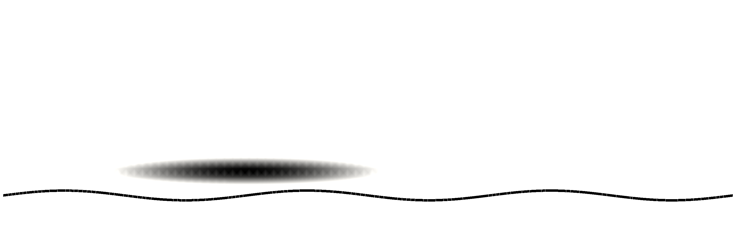
Figure 1: The volume force $f$ that generates the ’wind’ together with the zero level line of $\varphi_{0}$.

As parameters we choose $\rho_{water}=1$, $\eta_{water}=0.01$, $\sigma_{water}=0.0005$. Using unit velocity $V=1$ and unit length $d=1$, this results in a Weber number of $We=2000$ and after a required scaling due to the chosen free energy, see m6:AbelsGarckeGruen_CHNSmodell , we have $\sigma=0.00032$. The gravity is $g=(0.0,-9.81)^{\top}$ and the mobility is $b=\frac{\epsilon}{500\sigma}$. We note that especially the chosen density $\rho_{water}$ does not correspond to the real world parameter. We use the air-water ratio $\rho_{air}=0.01\rho_{water}$ and $\eta_{air}=0.01\eta_{water}$, which is ten times larger than the real world ratio. To overcome the limitations of the current implementation with respect to the density ratio is subject of future research.

For the adaptation process from Algorithm 1 we choose $\theta^{r}=0.5$, $\theta^{c}=0.01$, $V_{\min}=8e-6$, $V_{\max}=3e-4$. For the numerical results presented we switched off the postprocessing proposed in Algorithm 2. In m6:GarckeHinzeKahle_CHNS_AGG_linearStableTimeDisc the influence of this postprocessing on the numerical simulation of the rising bubble benchmark is investigated in detail.

In Fig. 2 we show snapshots of the evolution of the interface between water and air, given by the zero level line of $\varphi$, and the velocity field presented by streamlines of $v$, colored by $|v|$. We observe that, despite the unphysical parameters and boundary data, the method is able to deal with the complex two-phase interaction at the air-water interface.

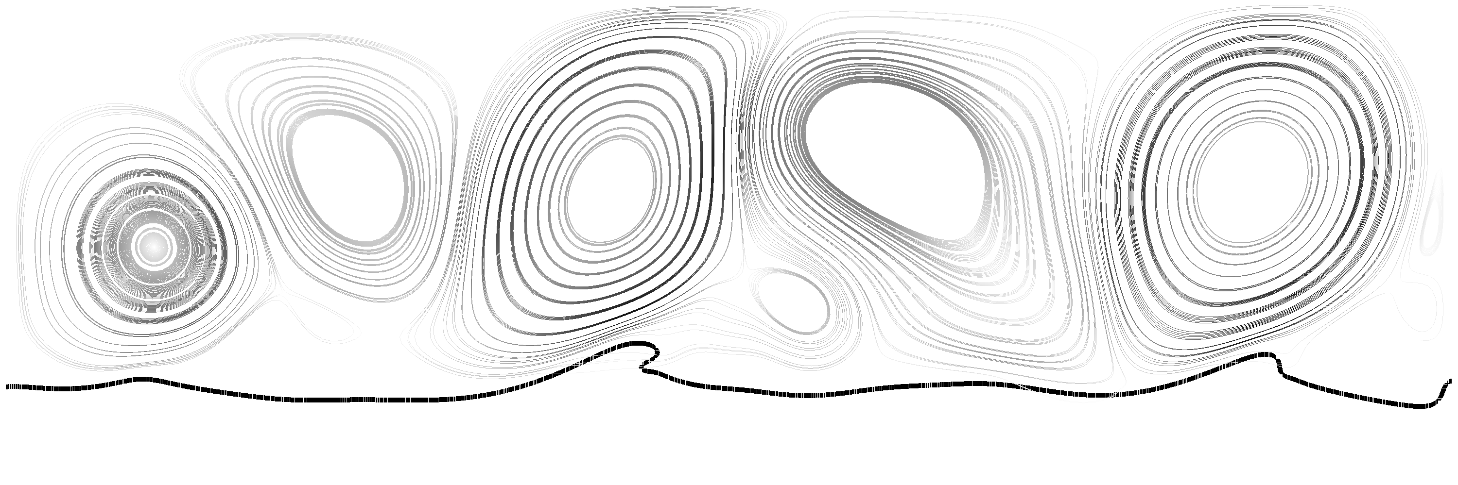
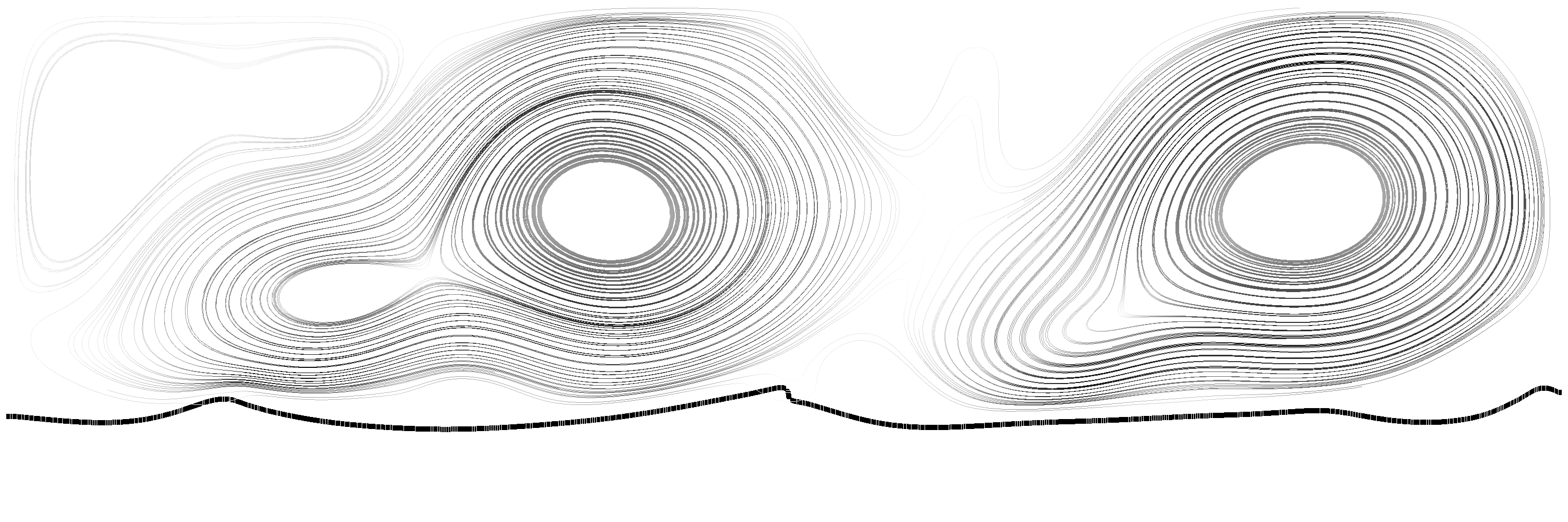
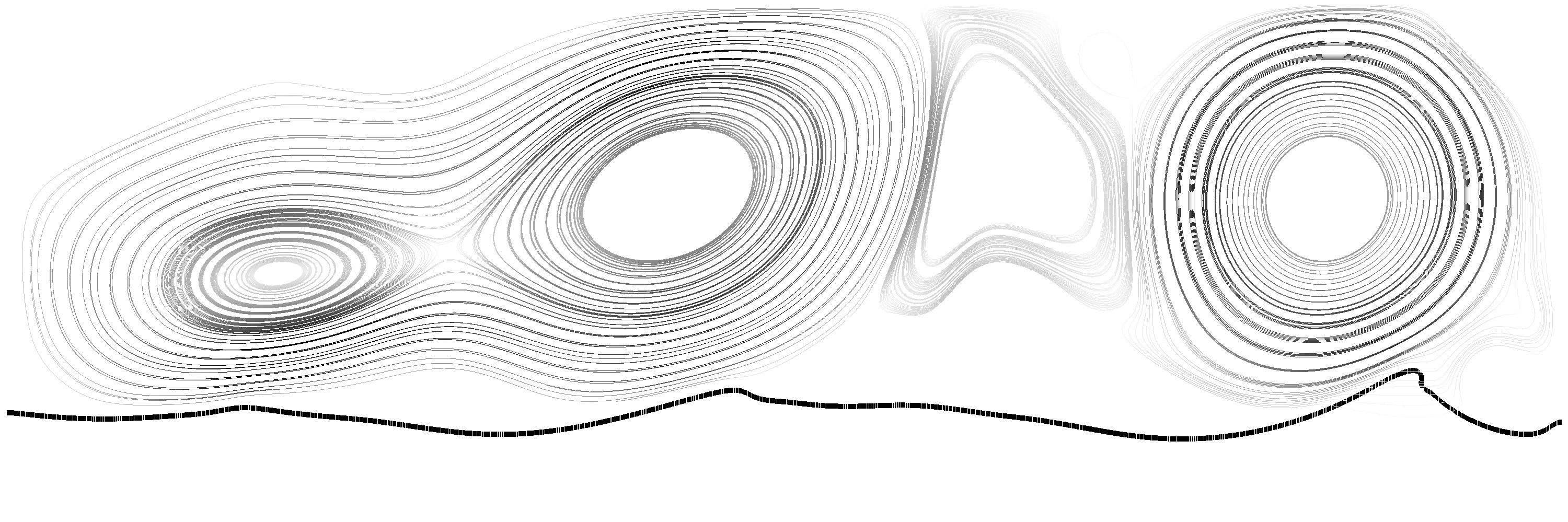
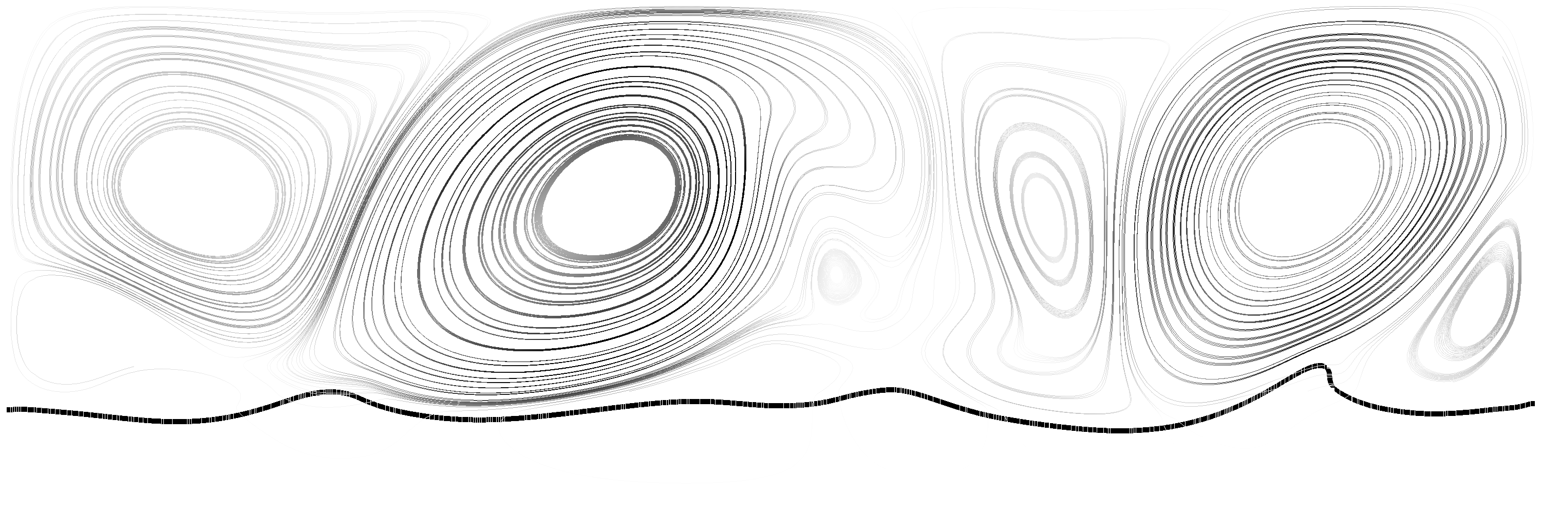
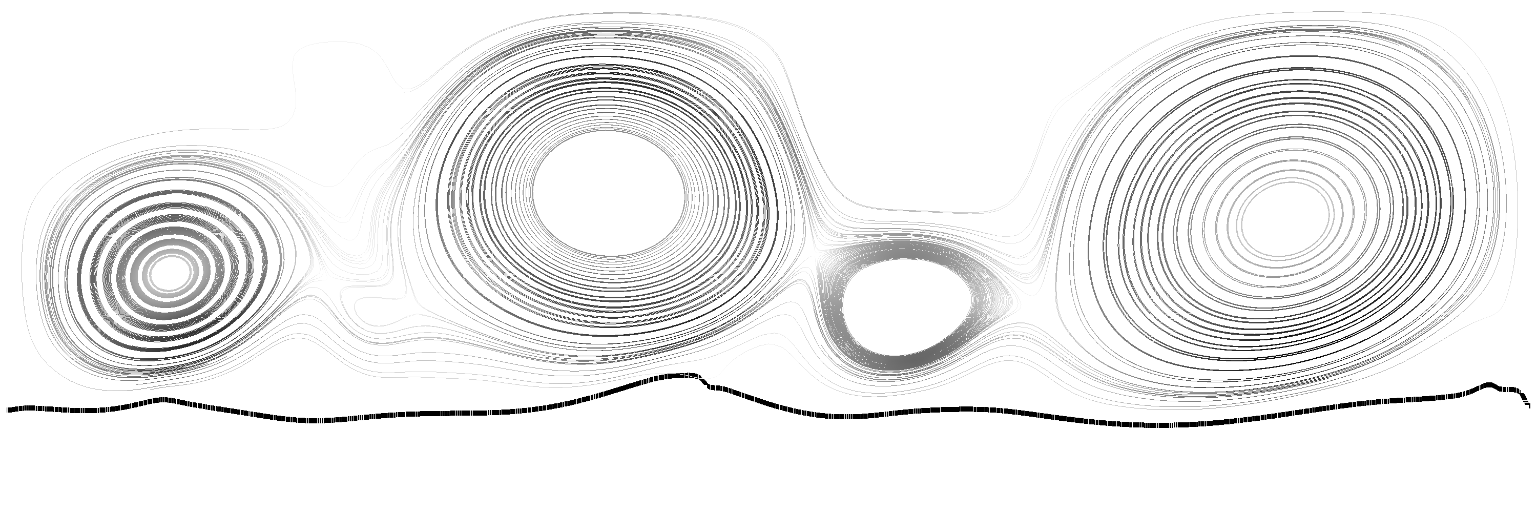
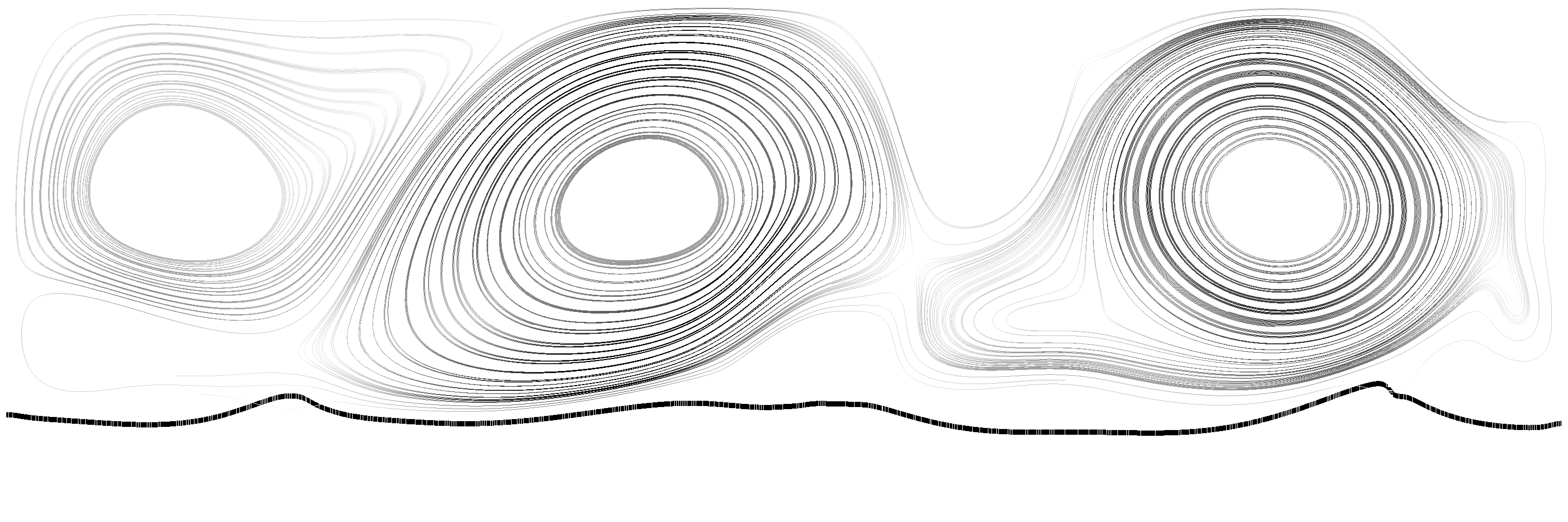
Figure 2: Snapshots of the evolution of $\varphi$ and $v$. For $t\in\{1.7,3.3,5.0,6.7,8.3,10.0$} (left top to right bottom) we present streamlines of $v$ in grayscale together with the zero level line of $\varphi$ in black. Darker streamlines means higher velocity. Due to the unphysical boundary data and the given forcing we observe large vortices that generate several waves at different locations. We stress, that especially breaking waves are captured by our approach as it is able to capture topological changes.

5 Outlook on the direction of research

The numerical results proposed in Sec. 4 are only preliminary and should be regarded as a proof of concept for the proposed diffuse interface approach. The method is able to cope with the complex phenomena at the air-water interface. Further research is necessary to further develop our approach, and to make it applicable for real world scenarios. This includes

Boundary data
As a first step the application of periodic boundary data for $v$ parallel to the water surface will be incorporated together with an open boundary on the top and the bottom of the domain. For $\varphi$ and $\mu$ periodic boundary conditions are sufficient in the water parallel directions only.

3D computations
For 3D computations an efficient solution of the linear systems arising troughout the simulation is essential. Here results on preconditioning of the Cahn–Hilliard system from m6:BoschStollBenner_fastSolutionCH or a multigrid approach as proposed in m6:KayWelford_multigridsolver might be used. For the solution of the Navier–Stokes equation well developed preconditioners exist and we refer to m6:Benzi_numericalSaddlePoint ; m6:kayLoghinWelford_FpPreconditioner .

Real world parameter
Incorporating real world parameters will require several changes on the architecture of the solver. Especially we note, that this will lead to large Reynolds number which require stabilization techniques like grad-div stabilization, which have to be encorporated into the finite element code. We note that the drawback of grad-div stabilization, namely a stronger coupling of the unknows, does not appear here, as in (1) all variables are coupled anyway due to the term $2Dv=\nabla v+(\nabla v)^{\top}$.

Incorporation into Earth System Models
If our concept proves applicable for the numerical simulation of the air-water region in atmosphere and ocean on the meter scale, it has to be incorporated into simulations on the next coarser (kilometer) scale. In this context homogenization concepts might be an option. We refer to e.g. m6:Eck2005 , where homogenization of phase field models has be done in a different context.

References

- [1] H. Abels, D. Depner, and H. Garcke. Existence of weak solutions for a diffuse interface model for two-phase flows of incompressible fluids with different densities. Journal of Mathematical Fluid Mechanics, 15(3):453–480, September 2013.
- [2] H. Abels, D. Depner, and H. Garcke. On an incompressible Navier–Stokes / Cahn–Hilliard system with degenerate mobility. Annales de l’Institut Henri Poincaré (C) Non Linear Analysis, 30(6):1175–1190, 2013.
- [3] H. Abels, H. Garcke, and G. Grün. Thermodynamically consistent, frame indifferent diffuse interface models for incompressible two-phase flows with different densities. Mathematical Models and Methods in Applied Sciences, 22(3):1150013(40), March 2012.
- [4] R. A. Adams and J. H. F. Fournier. Sobolev Spaces, second edition, volume 140 of Pure and Applied Mathematics. Elsevier, 2003.
- [5] G. L. Aki, W. Dreyer, J. Giesselmann, and C. Kraus. A quasi-incompressible diffuse interface model with phase transition. Mathematical Models and Methods in Applied Sciences, 24(5):827–861, May 2014.
- [6] S. Aland and A. Voigt. Benchmark computations of diffuse interface models for two-dimensional bubble dynamics. International Journal for Numerical Methods in Fluids, 69:747–761, 2012.
- [7] Aland, S., J. Lowengrub, and A. Voigt, 2010: Two-phase flow in complex geometries: A diffuse domain approach. CMES 57, 57(1), 77–108.
- [8] D. M. Anderson, G. B. McFadden, and A. A. Wheeler. Diffuse-interface methods in fluid mechanics. Annual Review of Fluid Mechanics, 30:139–165, 1998.
- [9] L. Baňas and R. Nürnberg. A posteriori estimates for the Cahn–Hilliard equation. Mathematical Modelling and Numerical Analysis, 3(5):1003 1026, 2009.
- [10] J.W. Barrett, H. Garcke, R. Nürnberg. A stable parametric finite element discretization of two-phase Navier-Stokes flow. J. Sci. Comput. 63(1):78-117, 2014.
- [11] M. Benzi, G.H. Golub, and J. Liesen. Numerical solution of saddle point problems. Acta Numerica, 14:1–137, 2005.
- [12] J. F. Blowey and C. M. Elliott. The Cahn–Hilliard gradient theory for phase separation with non-smooth free energy. Part I: Mathematical analysis. European Journal of Applied Mathematics, 2:233–280, 1991.
- [13] J. Bosch, M. Stoll, and P. Benner. Fast solution of Cahn-Hilliard Variational Inequalities using Implicit Time Discretization and Finite Elements. Journal of Computational Physics, 262:38–57, 2014.
- [14] F. Boyer. Mathematical study of multiphase flow under shear through order parameter formulation. Asymptotic Analysis, 20(2):175–212, 1999.
- [15] F. Boyer. A theoretical and numerical model for the study of incompressible mixture flows. Computers & Fluids, 31(1):41–68, January 2002.
- [16] F. Boyer, L. Chupin, and P. Fabrie. Numerical study of viscoelastic mixtures through a Cahn-Hilliard flow model. European Journal of Mechanics - B/Fluids, 23(5):759 – 780, 2004.
- [17] F. Boyer, C. Lapuerta, S. Minjeaud, B. Piar, and M. Quintard. Cahn–Hilliard/Navier–Stokes model for the simulation of three-phase flows. Transport in Porous Media, 82(3):463–483, April 2010.
- [18] L. Chen. FEM: An Innovative Finite Element Method Package in Matlab, available at: ifem.wordpress.com, 2008.
- [19] P. Clément. Approximation by finite element functions using local regularization. RAIRO Analyse numérique, 9(2):77–84, August 1975.
- [20] P. Constantin and C. Foias. Navier-Stokes-Equations. The University of Chicago Press, 1988.
- [21] H. Ding, P. D. M. Spelt, and C. Shu. Diffuse interface model for incompressible two-phase flows with large density ratios. Journal of Computational Physics, 226(2):2078–2095, October 2007.
- [22] Drennan, W., M. Donelan, E. Terray, and K. Katsaros, 1996: Oceanic turbulence dissipation measurements in SWADE. J. Phys. Oceanogr., 26, 808–815.
- [23] Druzhinin, O. A. and S. Elghobashi, 1998: Direct numerical simulations of bubble-laden turbulent flows using the two-fluid formulation. Phys. Fluids 10, 685–697.
- [24] C. Eck. Homogenization of phase field models for binary mixtures. SIAM Multicale Model. Simul. 3(1):1–27, 2004.
- [25] X. Feng. Fully Discrete Finite Element Approximations of the Navier–Stokes–Cahn–Hilliard Diffuse Interface Model for Two-Phase Fluid Flows. SIAM Journal on Numerical Analysis, 44(3):1049–1072, 2006.
- [26] Ganesan, S. and L. Tobiska, 2009: A coupled arbitrary lagrangian-eulerian and lagrangian method for computation of free surface flows with insoluble surfactants. Journal of Computational Physics, 228, 2859–2873.
- [27] H. Garcke, M. Hinze, and C. Kahle. A stable and linear time discretization for a thermodynamically consistent model for two-phase incompressible flow. Applied Numerical Mathematics, 99:151–171, January 2016.
- [28] S. Gross and A. Reusken. Numerical methods for two-phase incompressible flows, volume 40 of Springer Series in Computational Mathematics. Springer, 2011.
- [29] G. Grün. On convergent schemes for diffuse interface models for two-phase flow of incompressible fluids with general mass densities. SIAM Journal on Numerical Analysis, 51(6):3036–3061, 2013.
- [30] G. Grün, F. Guillén-Gonzáles, and S. Metzger. On Fully Decoupled Convergent Schemes for Diffuse Interface Models for Two-Phase Flow with General Mass Densities. Communications in Computational Physics, 19(5):1473–1502, May 2016.
- [31] G. Grün and F. Klingbeil. Two-phase flow with mass density contrast: Stable schemes for a thermodynamic consistent and frame indifferent diffuse interface model. Journal of Computational Physics, 257(A):708–725, January 2014.
- [32] Z. Guo, P. Lin, and J. S. Lowengrub. A numerical method for the quasi-incompressible Cahn–Hilliard–Navier–Stokes equations for variable density flows with a discrete energy law. Journal of Computational Physics, 276:486–507, November 2014.
- [33] M. Hintermüller, M. Hinze, and C. Kahle. An adaptive finite element Moreau–Yosida-based solver for a coupled Cahn–Hilliard/Navier–Stokes system. Journal of Computational Physics, 235:810–827, February 2013.
- [34] M. Hintermüller, M. Hinze, and M. H. Tber. An adaptive finite element Moreau–Yosida-based solver for a non-smooth Cahn–Hilliard problem. Optimization Methods and Software, 25(4-5):777–811, 2011.
- [35] S. Hysing, S. Turek, D. Kuzmin, N. Parolini, E. Burman, S. Ganesan, and L. Tobiska. Quantitative benchmark computations of two-dimensional bubble dynamics. International Journal for Numerical Methods in Fluids, 60(11):1259–1288, 2009.
- [36] James, A. J. and J. Lowengrub, 2004: A surfactant-conserving volume-of-fluid method for interfacial flows with insoluble surfactant. J. Comput. Phys., 201(2), 685–722.
- [37] C. Kahle. Simulation and Control of Two-Phase Flow Using Diffuse-Interface Models. PhD thesis, University of Hamburg, 2014.
- [38] D. Kay, D. Loghin, and A. Wathen. A preconditioner for the steady state Navier–Stokes equations. SIAM Journal on Scientific Computing, 24(1):237–256, 2002.
- [39] D. Kay, V. Styles, and R. Welford. Finite element approximation of a Cahn–Hilliard–Navier–Stokes system. Interfaces and Free Boundaries, 10(1):15–43, 2008.
- [40] D. Kay and R. Welford. A multigrid finite element solver for the Cahn–Hilliard equation. Journal of Computational Physics, 212:288–304, 2006.
- [41] D. Kay and R. Welford. Efficient numerical solution of Cahn-Hilliard-Navier-Stokes fluids in 2d. SIAM J. on Scientific Computing, 29(6):2241—2257, 2007.
- [42] Kihara, N., H. Hanazaki, T. Mizuya, and H. Ueda, 2007: Relationship between airflow at the critical height and momentum transfer to the traveling waves. Phys. Fluids, 19 (015102).
- [43] Kim, J., 2012: Phase-field models for multi-component fluid flows. Commun. Comput. Physics 12, 613–661.
- [44] J. Lowengrub and L. Truskinovsky. Quasi-incompressible Cahn–Hilliard fluids and topological transitions. Proceedings of the royal society A, 454(1978):2617–2654, 1998.
- [45] Lubin, P. and S. Glockner, 2015: Numerical simulations of three-dimensional plunging breaking waves: generation and evolution of aerated vortex filaments. J. Fluid Mech., 767, 364–393.
- [46] McWilliams, J., P. Sullivan, and C. Moeng, 1997: Langmuir turbulence in the ocean. J. Fluid Mech., 334, 1–30.
- [47] Mellado, J. P., B. Stevens, H. Schmidt and N. Peters, 2010: Two–fluid formulation of the cloud-top mixing layer for direct numerical simulation. Theor. Comput. Fluid Dyn., 24, 511–536.
- [48] Polton, J., J. Smith, J. MacKinnon, and A. Tejada-Martinez, 2008: Rapid generation of high frequency internal waves beneath a wind wave forced oceanic surface mixed layer. Geophys. Res. Lett., (L13602).
- [49] Shen, L., X. Zhang, D. Yue, and M. Triantafyllou, 2003: Turbulent flow over a flexible wall undergoing a streamwise travelling wave motion. J. Fluid Mech., 484, 197–221.
- [50] Sullivan, P. and J. McWilliams, 2002: Turbulent flow over water waves in the presence of stratification. Phys. Fluids, 14, 1182–95.
- [51] Sullivan, P. and J. McWilliams, 2010: Dynamics of winds and currents coupled to surface waves. Ann. Rev. Fluid Mech., 42, 19–42.
- [52] Sullivan, P., J. McWilliams, and W. Melville, 2007: Surface gravity wave effects in the oceanic boundary layer: large-eddy simulation with vortex force and stochastic breakers. J. Fluid Mech., 593, 405–452.
- [53] Sullivan, P., J. McWilliams, and C. Moeng, 2000: Simulation of turbulent flow over idealized water waves. J. Fluid Mech., 404, 47–85.
- [54] Sutherland, P. and W. Melville, 2015: Field measurements of surface and near-surface turbulence in the presence of breaking waves. J. Phys. Oceanogr., 45, 943–965.
- [55] Tsai, W., S. Chen, and G. Lu, 2015: Numerical evidence of turbulence generated by nonbreaking surface waves. J. Phys. Oceanogr., 45, 174–180.
- [56] Tsai, W. and L. Hung, 2007: Three-dimensional modeling of small-scale processes in the upper boundary layer bounded by a dynamic ocean surface. J. Geophys. Res., 112 (C02019).
- [57] Wan, D.; Turek, S., 2007: An efficient multigrid-FEM method for the simulation of solid-liquid two phase flows. J. Comp. Appl. Math., 203(2), 561-580.
- [58] R. Verfürth. A posteriori error analysis of space-time finite element discretizations of the time-dependent Stokes equations. Calcolo, 47:149–167, 2010.
- [59] Wunsch, C. and R. Ferrari, 2004: Vertical mixing, energy, and the general circulation of the oceans. Ann. Rev. Fluid Mech., 36, 281–314.