An $hp$–Adaptive Newton-Discontinuous-Galerkin Finite Element Approach for Semilinear Elliptic Boundary Value Problems

Abstract.

In this paper we develop an $hp$–adaptive procedure for the numerical solution of general second-order semilinear elliptic boundary value problems, with possible singular perturbation. Our approach combines both adaptive Newton schemes and an $hp$–version adaptive discontinuous Galerkin finite element discretisation, which, in turn, is based on a robust $hp$–version a posteriori residual analysis. Numerical experiments underline the robustness and reliability of the proposed approach for various examples.

1. Introduction

The subject of this paper is the adaptive numerical approximation of second-order semilinear elliptic problems of the form

$$-\epsilon\Delta u+u =f(\cdot,u)\text{ in }\ \Omega,\qquad u=0\text{ on }\partial\Omega.$$ (1)

Here, $\Omega\subset\mathbb{R}^{2}$ is an open and bounded Lipschitz domain, $\epsilon\in(0,1]$ represents a (possibly small singular perturbation) parameter, $f:\,\overline{\Omega}\times\mathbb{R}\to\mathbb{R}$ is a continuously differentiable function, and $u:\,\Omega\to\mathbb{R}$ is an unknown solution; in the sequel, we will omit to explicitly express the dependence of $f$ on the first argument, and simply write $f(u)$ instead. Problems of this type appear in a wide range of application areas of practical interest, such as, for example, nonlinear reaction-diffusion in ecology and chemical models [14, 24, 12, 42, 43], economy [8], or classical and quantum physics [10, 29, 9, 48].

Partial differential equations (PDEs) of the form (1) may admit a unique solution, no solution at all, or more typically a multitude of solutions, or indeed infinitely many such solutions. Moreover, in the singularly perturbed case, i.e., when $0<\epsilon\ll 1$, solutions of (1), when they exist, may contain sharp layers in the form of interior/boundary layers, or isolated spike–like solutions, and their numerical approximation represents a challenging computational task. Indeed, to efficiently and reliably compute discrete approximations to the analytical solution $u$ of (1), it is essential to exploit a posteriori bounds which not only provide information regarding the size of the discretisation error, measured in some appropriate norm, but also yield local error indicators which may subsequently be employed to enrich the underlying approximation space in an adaptive manner. Of course, a key aspect of this general solution procedure is the design and implementation of a nonlinear solver which can efficiently compute the approximation $u_{h}$ to $u$; we shall return to this issue below.

In general, the traditional approach exploited within the literature for the design of adaptive finite element methods, for example, is to first discretise the underlying PDE problem, in our case (1), and to derive an a posteriori error bound for the resulting (nonlinear) scheme; this is typically a very mathematically challenging task. However, once such a bound has been established, then given a suitable initial mesh and polynomial approximation order, the underlying nonlinear system of discrete equations arising from the underlying finite element discretisation may be solved based on employing, for example, a (damped) Newton iteration. Denoting this computed numerical approximation by $u_{h}$, the size of the error between $u$ and $u_{h}$ may then be estimated by exploiting this a posteriori error bound. If this bound is below a given user tolerance, then sufficient accuracy has been attained and the adaptive algorithm may be terminated. Otherwise, the computational mesh ($h$–refinement) or the polynomial degree ($p$–refinement), or both ($hp$–refinement) are locally enriched based on identifying regions in the domain where the elementwise error indicators, which stem from the a posteriori error bound, are locally large. On the basis of this new finite element space, a new approximation $u_{h}$ to $u$ may be computed, and the whole process repeated until either the desired accuracy has been attained, or a maximum number of refinement steps have been completed.

Stimulated by the work undertaken in the recent article [5], we consider an alternative approach based on the so-called adaptive Newton-Galerkin paradigm for the numerical approximation of nonlinear problems of the type (1). More precisely, this general technique is based on applying local Newton-type linearisations on the continuous level that allow for the approximation of the semilinear PDE (1) by a sequence of linearised problems. These resulting linear PDEs are then discretised by means of an adaptive finite element procedure, which, in turn, is based on a suitable a posteriori residual analysis. The adaptive Newton-Galerkin procedure provides an interplay between the (adaptive, or damped) Newton method and the adaptive finite element approach, whereby we either perform a Newton step (if the Newton linearisation effect dominates) or enrich the current finite element space based on the above a posteriori residual indicators (in the case that the finite element discretisation constitutes the main source of error); for related work we refer to [16, 26], or the articles [11, 21, 28] on (derivative-free) fixed-point iteration schemes. Finally, we point to the works [15, 30] dealing with modelling errors in linearised models.

In the current article, we extend the work undertaken in [5] to the framework of $hp$–version adaptive interior penalty discontinuous Galerkin (DG) schemes, thereby giving rise to $hp$–adaptive Newton-discontinuous Galerkin (NDG) methods. Here, the proof of the resulting a posteriori residual bound for the interior penalty DG discretisation of the underlying linearised PDE problem is based on two key steps: firstly, we introduce a suitable residual operator on a given enriched space, which, when measured in an appropriate norm, is equivalent to the error measured in terms of the underlying DG energy norm. Secondly, an upper bound on the norm of the residual operator is derived based on exploiting the general techniques developed in the articles [32, 31, 51]; we also refer to [52] for the application to convection–diffusion problems, and to [35, 19] for the treatment of strongly monotone quasilinear PDEs, cf., also, [20, 18] for $hp$–version two-grid DG methods. The proof of this upper bound crucially relies on the approximation of discontinuous finite element functions by conforming ones, cf., also, [37] for the $h$–version case. Moreover, in the current setting, following [49], particular care is devoted to the derivation of $\epsilon$-robust approximation estimates. The resulting a posteriori bound consists of two key terms: one stemming from the Newton linearisation error, and the second which measures the approximation error in the underlying DG scheme. On the basis of this general $hp$–version bound, we devise a fully automatic $hp$–adaptive NDG scheme for the numerical approximation of PDEs of the form (1). Indeed, the performance of the resulting adaptive strategy is demonstrated on both the Bratu and Ginzburg Landau problems; moreover, the superiority of exploiting $hp$–enrichment of the DG finite element space, in comparison with standard mesh adaptation ($h$–refinement), will be highlighted.

The structure of this article is as follows. In Section 2 we briefly outline the adaptive (damped) Newton linearisation procedure employed within this article. The $hp$–version interior penalty DG discretisation of the resulting linearised PDE problem is then given in Section 3. Section 4 is devoted to the derivation of a residual-based a posteriori bound. On the basis of this bound in Section 5 we design a suitable adaptive refinement strategy, which controls both the error arising in the Newton linearisation, as well as the error in the $hp$–DG finite element scheme; in the latter case, we exploit automatic $hp$–refinement of the underlying finite element space. The performance of this proposed algorithm is demonstrated for a series of numerical examples presented in Section 6. Finally, in Section 7 we summarise the work presented in this article and discuss potential future extensions.

2. Newton Linearisation

2.1. An Adaptive Newton Approach

We will briefly revisit an adaptive ‘black-box’ prediction-type Newton algorithm from [5], and refer to [23] for more sophisticated approaches in more specific situations. Let us consider two Banach spaces $X,Y$, with norms $\|\cdot\|_{X}$ and $\|\cdot\|_{Y}$, respectively. Then, given an open subset $\Xi\subset X$, and a (possibly nonlinear) operator $\mathsf{F}_{\epsilon}:\,\Xi\to Y$, we are interested in solving the nonlinear operator equation

$$\mathsf{F}_{\epsilon}(u)=0,$$ (2)

for some unknown zeros $u\in\Xi$. Supposing that the Fréchet derivative $\mathsf{F}_{\epsilon}^{\prime}$ of $\mathsf{F}_{\epsilon}$ exists in $\Xi$ (or in a suitable subset), the classical Newton method for solving (2) starts from an initial guess $u_{0}\in\Xi$, and generates a sequence $\{u_{n}\}_{n\geq 1}\subset X$ that is defined iteratively by the linear equation

$$\mathsf{F}_{\epsilon}^{\prime}(u_{n})(u_{n+1}-u_{n})=-\mathsf{F}_{\epsilon}(u_{n}),\qquad n\geq 0.$$ (3)

Naturally, for this iteration to be well-defined, we need to assume that $\mathsf{F}_{\epsilon}^{\prime}(u_{n})$ is invertible for all $n\geq 0$, and that $\{u_{n}\}_{n\geq 0}\subset\Xi$.

In order to improve the reliability of the Newton method (3) in the case that the initial guess $u_{0}$ is relatively far away from a root $u_{\infty}\in\Xi$ of $\mathsf{F}_{\epsilon}$, $\mathsf{F}_{\epsilon}(u_{\infty})=0$, introducing some damping in the Newton method is a well-known remedy. In that case (3) is rewritten as

$$u_{n+1}=u_{n}-\Delta t_{n}\mathsf{F}_{\epsilon}^{\prime}(u_{n})^{-1}\mathsf{F}_{\epsilon}(u_{n}),\qquad n\geq 0,$$ (4)

where $\Delta t_{n}>0$, $n\geq 0$, is a damping parameter that may be adjusted adaptively in each iteration step. The selection of the Newton parameter $\Delta t_{n}$ is based on the following idea from [5]: provided that $\mathsf{F}_{\epsilon}^{\prime}(u)$ is invertible on a suitable subset of $\Xi\subset X$, we define the Newton-Raphson transform by

$$u\mapsto\mathsf{NF}(u):=-\mathsf{F}_{\epsilon}^{\prime}(u)^{-1}\mathsf{F}_{\epsilon}(u);$$

see, e.g., [44]. Then, rearranging terms in (4), we notice that

$$\frac{u_{n+1}-u_{n}}{\Delta t_{n}}=\mathsf{NF}(u_{n}),\qquad n\geq 0,$$

i.e., (4) can be seen as the discretisation of the dynamical system

$$\begin{split}\dot{u}(t)&=\mathsf{NF}(u(t)),\quad t\geq 0,\qquad u(0)=u_{0},\end{split}$$ (5)

by the forward Euler scheme, with step size $\Delta t_{n}>0$. For $t\in[0,\infty)$, the solution $u(t)$ of (5), if it exists, defines a trajectory in $X$ that starts at $u_{0}$, and that will potentially converge to a zero of $\mathsf{F}_{\epsilon}$ as $t\to\infty$. Indeed, this can be seen (formally) from the integral form of (5), that is,

$$\mathsf{F}_{\epsilon}(u(t))=\mathsf{F}_{\epsilon}(u_{0})e^{-t},\qquad t\geq 0,$$

which implies that $\mathsf{F}_{\epsilon}(u(t))\to 0$ as $t\to\infty$.

Now taking the view of dynamical systems, our goal is to compute an upper bound for the value of the step sizes $\Delta t_{n}>0$ from (4), $n\geq 0$, so that the discrete forward Euler solution $\{u_{n}\}_{n\geq 0}$ from (4) stays reasonably close to the continuous solution of (5). Specifically, for a prescribed tolerance $\tau>0$, a Taylor expansion analysis (see [5, Section 2] for details) reveals that

$$u(t)=u_{0}+t\mathsf{NF}(u_{0})+\frac{t^{2}}{2h}\eta_{h}+\mathcal{O}(t^{3})+\mathcal{O}(t^{2}h\|\mathsf{NF}(u_{0})\|_{X}^{2}),$$

where, for any sufficiently small $h>0$, we let $\eta_{h}=\mathsf{NF}(u_{0}+h\mathsf{NF}(u_{0}))-\mathsf{NF}(u_{0})$. Hence, after the first time step of length $\Delta t_{0}>0$ there holds

$$u(\Delta t_{0})-u_{1}=\frac{\Delta t_{0}^{2}}{2h}\eta_{h}+\mathcal{O}(\Delta t_{0}^{3})+\mathcal{O}(\Delta t_{0}^{2}h\|\mathsf{NF}(u_{0})\|_{X}^{2}),$$ (6)

where $u_{1}$ is the forward Euler solution from (4). Therefore, upon setting

$$\Delta t_{0}=\sqrt{2\tau h\|\eta_{h}\|_{X}^{-1}},$$

we arrive at

$$\|u(\Delta t_{0})-u_{1}\|_{X}\leq\tau+\mathcal{O}(\Delta t_{0}^{3})+\mathcal{O}(\Delta t_{0}^{2}h\|\mathsf{NF}(u_{0})\|_{X}^{2}).$$

In order to balance the $\mathcal{O}$-terms in (6) it is sensible to make the choice

$$h=\mathcal{O}(\Delta t_{0}\|\mathsf{NF}(u_{0})\|_{X}^{-2}),$$

i.e.,

$$h=\gamma\Delta t_{0}\|\mathsf{NF}(u_{0})\|_{X}^{-2},$$ (7)

for some parameter $\gamma>0$. This leads to the following adaptive Newton algorithm.

Algorithm 2.1.

Fix a tolerance $\tau>0$ as well as a parameter $\gamma>0$, and set $n\leftarrow 0$.

1:Start the Newton iteration with an initial guess $u_{0}\in\Xi$.

2:if $n=0$ then choose

$$\Delta t_{0}=\min\left\{\sqrt{2\tau\left\|\mathsf{NF}(u_{0})\right\|_{X}^{-1}},1\right\},$$

based on [5, Algorithm 2.1] (cf. also [4]),

3:else if $n\geq 1$ then let $\kappa_{n}=\Delta t_{n-1}$, and $h_{n}=\gamma\kappa_{n}\|\mathsf{NF}(u_{n})\|_{X}^{-2}$ based on (7); define the Newton step size

$$\Delta t_{n}=\min\left\{\sqrt{2\tau h_{n}\left\|\mathsf{NF}(u_{n}+h_{n}\mathsf{NF}(u_{n}))-\mathsf{NF}(u_{n})\right\|^{-1}_{X}},1\right\}.$$ (8)

4:end if

5:Compute $u_{n+1}$ based on the Newton iteration (4), and go to (3:) with $n\leftarrow n+1$.

We notice that the minimum in (8) ensures that the step size $\Delta t_{n}$ is chosen to be 1 whenever possible. Indeed, this is required in order to guarantee quadratic convergence of the Newton iteration close to a root (provided that the root is simple). Furthermore, we remark that the prescribed tolerance $\tau$ in the above adaptive strategy will typically be fixed a priori. Here, for highly nonlinear problems featuring numerous or even infinitely many solutions, it is typically mandatory to select $\tau\ll 1$ small in order to remain within the attractor of the given initial guess. This is particularly important if the starting value is relatively far away from a solution.

2.2. Application to Semilinear PDEs

In this article, we suppose that a (not necessarily unique) solution $u\in X:=H^{1}_{0}(\Omega)$ of (1) exists; here, we denote by $H^{1}_{0}(\Omega)$ the standard Sobolev space of functions in $H^{1}(\Omega)=W^{1,2}(\Omega)$ with zero trace on $\partial\Omega$. Furthermore, signifying by $X^{\prime}=H^{-1}(\Omega)$ the dual space of $X$, and upon defining the map $\mathsf{F}_{\epsilon}:X\rightarrow X^{\prime}$ through

$$\left\langle\mathsf{F}_{\epsilon}(u),v\right\rangle:=\int_{\Omega}\left\{\epsilon\nabla u\cdot\nabla v+uv-f(u)v\right\}\,\mathsf{d}\bm{x}\qquad\forall v\in X,$$ (9)

where $\left\langle\cdot,\cdot\right\rangle$ is the dual product in $X^{\prime}\times X$, the above problem (1) can be written as a nonlinear operator equation in $X^{\prime}$:

$$u\in X:\qquad\mathsf{F}_{\epsilon}(u)=0.$$ (10)

For any subset $D\subseteq\Omega$, we denote by $\|\cdot\|_{0,D}$ the $L^{2}$-norm on $D$; in the case when $D=\Omega$, we simply write $\|\cdot\|_{0}$ in lieu of $\|\cdot\|_{0,\Omega}$. With this notation, we note that the space $X$ is equipped with the norm

$$\|u\|^{2}_{X}:=\epsilon\|\nabla u\|^{2}_{0}+\|u\|_{0}^{2},\qquad u\in X.$$

The Fréchet-derivative of the operator $\mathsf{F}_{\epsilon}$ from (10) at $u\in X$ is given by

$$\left\langle\mathsf{F}_{\epsilon}^{\prime}(u)w,v\right\rangle=\int_{\Omega}\left\{\epsilon\nabla w\cdot\nabla v+wv-f^{\prime}(u)wv\right\}\,\mathsf{d}\bm{x},\qquad v,w\in X=H^{1}_{0}(\Omega),$$

where we write $f^{\prime}\equiv\partial_{u}f$. We note that, if there is a constant $\omega>1$ for which $f^{\prime}(u)\in L^{\omega}(\Omega)$, then $\mathsf{F}_{\epsilon}^{\prime}(u)$ is a well-defined linear and bounded mapping from $X$ to $X^{\prime}$; see [5, Lemma A.1].

Now given an initial guess $u_{0}\in X$, the adaptive Newton method (4) for (10) is defined iteratively to find $u_{n+1}\in X$ from $u_{n}\in X$, $n\geq 0$, such that

$$\mathsf{F}_{\epsilon}^{\prime}(u_{n})(u_{n+1}-u_{n})=-\Delta t_{n}\mathsf{F}_{\epsilon}(u_{n}),$$

in $X^{\prime}$. When applied to (9) and (10), this turns into

$$\int_{\Omega}\{\epsilon\nabla(u_{n+1}-u_{n}) \cdot\nabla v+(u_{n+1}-u_{n})v-f^{\prime}(u_{n})(u_{n+1}-u_{n})v\}\,\mathsf{d}\bm{x}$$

$$=-\Delta t_{n}\int_{\Omega}\left\{\epsilon\nabla u_{n}\cdot\nabla v+u_{n}v-f(u_{n})v\right\}\,\mathsf{d}\bm{x}\qquad\forall v\in X.$$

Hence, for $n\geq 0$, the updated Newton iterate $u_{n+1}$ is defined through the linear weak formulation

$$\begin{split}\int_{\Omega}\{\epsilon\nabla\widehat{\mathfrak{u}}_{n+1}\cdot\nabla v&+\widehat{\mathfrak{u}}_{n+1}v-f^{\prime}(u_{n})\widehat{\mathfrak{u}}_{n+1}v\}\,\mathsf{d}\bm{x}=\Delta t_{n}\int_{\Omega}\{f(u_{n})-f^{\prime}(u_{n})u_{n}\}v\,\mathsf{d}\bm{x}\qquad\forall v\in X,\end{split}$$ (11)

where $\widehat{\mathfrak{u}}_{n+1}=u_{n+1}-(1-\Delta t_{n})u_{n}$. Incidentally, if there exists a constant $\delta$ with $\epsilon^{-1}(f^{\prime}(u_{n})-1)\leq\delta<C_{\text{\tiny\sf{PF}}}^{-2}$ on $\Omega$, where $C_{\text{\tiny\sf{PF}}}=C_{\text{\tiny\sf{PF}}}(\Omega)>0$ is the constant in the Poincaré-Friedrichs inequality on $\Omega$,

$$\|w\|_{0}\leq C_{\text{\tiny\sf{PF}}}\|\nabla w\|_{0}\qquad\forall w\in X,$$

then (11) is a linear second-order diffusion-reaction problem that is coercive on $X$. In particular, (11) exhibits a unique solution $u_{n+1}\in X$ in this case.

3. $hp$–DG Discretisation

3.1. Meshes, Spaces, and DG Flux Operators

We will employ a standard $hp$–DG setting; see, e.g., [32, 52].

3.1.1. Meshes and DG Spaces

Let $\mathcal{T}$ be a subdivision of $\Omega$ into disjoint open parallelograms $\kappa$ such that $\overline{\Omega}=\bigcup_{\kappa\in\mathcal{T}}{\overline{\kappa}}$. We assume that $\mathcal{T}$ is shape-regular, and that each $\kappa\in\mathcal{T}$ is an affine image of the unit square $\widehat{\kappa}=(0,1)^{2}$; i.e., for each $\kappa\in\mathcal{T}$ there exists an affine element mapping $\Psi_{\kappa}:\,\widehat{\kappa}\to\kappa$ such that $\kappa=\Psi_{\kappa}({\widehat{\kappa}})$. By $h_{\kappa}$ we denote the element diameter of $\kappa\in\mathcal{T}$, $h=\max_{\kappa\in{\mathcal{T}}_{h}}h_{\kappa}$ is the mesh size, and $\bm{n}_{\kappa}$ signifies the unit outward normal vector to $\kappa$ on $\partial\kappa$. Furthermore, we assume that $\mathcal{T}$ is of bounded local variation, i.e., there exists a constant $\rho_{1}\geq 1$, independent of the element sizes, such that $\rho_{1}^{-1}\leq\nicefrac{{h_{\kappa}}}{{h_{\kappa^{\prime}}}}\leq\rho_{1}$, for any pair of elements $\kappa,\kappa^{\prime}\in\mathcal{T}$ which share a common edge $e=(\partial\kappa\cap\partial\kappa^{\prime})^{\circ}$. In this context, let us consider the set ${\mathcal{E}}$ of all one-dimensional open edges of all elements $\kappa\in\mathcal{T}$. Further, we denote by $\mathcal{E}_{\mathcal{I}}$ the set of all edges $e$ in $\mathcal{E}$ that are contained in $\Omega$ (interior edges). Additionally, introduce ${\mathcal{E}}_{\mathcal{B}}$ to be the set of boundary edges consisting of all $e\in{\mathcal{E}}$ that are contained in $\partial\Omega$. In our analysis, we allow the meshes to be 1-irregular, i.e., each edge of an element $\kappa\in\mathcal{T}$ may contain (at most) one hanging node, which we assume to be located at the centre of $e$. Suppose that $e$ is an edge of an element $\kappa\in\mathcal{T}$; then, by $h_{e}$, we denote the length of $e$. Due to our assumptions on the subdivision $\mathcal{T}$ we have that, if $e\subset\partial\kappa$, then $h_{e}$ is commensurate with $h_{\kappa}$, the diameter of $\kappa$.

For a nonnegative integer $k$, we denote by ${\mathcal{Q}}_{k}({\widehat{\kappa}})$ the set of all tensor-product polynomials on $\widehat{\kappa}$ of degree $k$ in each co-ordinate direction. To each $\kappa\in\mathcal{T}$ we assign a polynomial degree $p_{\kappa}$ (local approximation order). We store the quantities $h_{\kappa}$ and $p_{\kappa}$ in the vectors ${\bm{h}}=\{h_{\kappa}:\,\kappa\in\mathcal{T}\}$ and ${\bm{p}}=\{p_{\kappa}:\,\kappa\in\mathcal{T}\}$, respectively, and consider the DG finite element space

$$\mathcal{V}_{\text{\tiny\sf{DG}}}=\{v\in L^{2}(\Omega):\;v|_{\kappa}\circ\Psi_{\kappa}\in{\mathcal{Q}}_{p_{\kappa}}(\widehat{\kappa})\quad\forall\kappa\in\mathcal{T}\}\;.$$ (12)

We shall suppose that the polynomial degree vector $\mathbf{p}$, with $p_{\kappa}\geq 1$ for each $\kappa\in\mathcal{T}$, has bounded local variation, i.e., there exists a constant $\rho_{2}\geq 1$ independent of $\bm{h}$ and $\bm{p}$, such that, for any pair of neighbouring elements $\kappa,\kappa^{\prime}\in\mathcal{T}$, we have $\rho_{2}^{-1}\leq\nicefrac{{p_{\kappa}}}{{p_{\kappa^{\prime}}}}\leq\rho_{2}$. Moreover, for an edge $e=(\partial\kappa\cap\partial\kappa^{\prime})^{\circ}$ shared by two elements $\kappa,\kappa^{\prime}\in\mathcal{T}$, we define $p_{e}:=\nicefrac{{1}}{{2}}(p_{\kappa}+p_{\kappa^{\prime}})$, or $p_{e}=p_{\kappa}$ if $e=(\partial\kappa\cap\partial\Omega)^{\circ}$, for some $\kappa\in\mathcal{T}$, is a boundary edge.

3.1.2. Jump and Average Operators

Let $\kappa$ and $\kappa^{\prime}$ be two adjacent elements of  $\mathcal{T}$, and $\bm{x}$ an arbitrary point on the interior edge $e\in\mathcal{E}_{\mathcal{I}}$ given by $e=(\partial\kappa\cap\partial\kappa^{\prime})^{\circ}$. Furthermore, let $v$ and $\bm{q}$ be scalar- and vector-valued functions, respectively, that are sufficiently smooth inside each element $\kappa,\kappa^{\prime}$. Then, the averages of $v$ and $\bm{q}$ at $\bm{x}\in e$ are given by

$$\langle\!\langle v\rangle\!\rangle=\frac{1}{2}(v|_{\kappa}+v|_{\kappa^{\prime}}),\qquad\langle\!\langle\bm{q}\rangle\!\rangle=\frac{1}{2}(\bm{q}|_{\kappa}+\bm{q}|_{\kappa^{\prime}}),$$

respectively. Similarly, the jumps of $v$ and $\bm{q}$ at $\bm{x}\in e$ are given by

$$[\![v]\!]=v|_{\kappa}\,\bm{n}_{\kappa}+v|_{\kappa^{\prime}}\,\bm{n}_{\kappa^{\prime}},\qquad[\![\bm{q}]\!]=\bm{q}|_{\kappa}\cdot\bm{n}_{\kappa}+\bm{q}|_{\kappa^{\prime}}\cdot\bm{n}_{\kappa^{\prime}},$$

respectively. On a boundary edge $e\in\mathcal{E}_{\mathcal{B}}$, we set $\langle\!\langle v\rangle\!\rangle=v$, $\langle\!\langle\bm{q}\rangle\!\rangle=\bm{q}$ and $[\![v]\!]=v\bm{n}$, with $\bm{n}$ denoting the unit outward normal vector on the boundary $\partial\Omega$.

Furthermore, we introduce, for an edge $e\in{\mathcal{E}}$, the discontinuity penalisation parameter $\sigma$ by

$$\sigma|_{e}=\frac{p_{e}^{2}}{h_{e}}.$$ (13)

We conclude this section by equipping the DG space $\mathcal{V}_{\text{\tiny\sf{DG}}}$ with the DG norm

$$\left\|v\right\|_{\text{\tiny\sf{DG}}}^{2}:=\epsilon\left\|\nabla_{\mathcal{T}}v\right\|^{2}_{0}+\left\|v\right\|^{2}_{0}+\int_{\mathcal{E}}(\epsilon\sigma+\sigma^{-1})|[\![v]\!]|^{2}\,\mathsf{d}s,$$ (14)

which is induced by the DG inner product

$$(v,w)_{\text{\tiny\sf{DG}}}=\int_{\Omega}\left\{\epsilon\nabla_{\mathcal{T}}v\cdot\nabla_{\mathcal{T}}w+vw\right\}\,\mathsf{d}\bm{x}+\int_{\mathcal{E}}(\epsilon\sigma+\sigma^{-1})[\![w]\!]\cdot[\![v]\!]\,\mathsf{d}s.$$ (15)

Here, $\nabla_{\mathcal{T}}$ is the element-wise gradient operator. For an element $\kappa\in\mathcal{T}$ we shall also use the norm

$$\|v\|_{\epsilon,\kappa}^{2}:=\epsilon\left\|\nabla v\right\|^{2}_{0,\kappa}+\left\|v\right\|^{2}_{0,\kappa},$$

for $v\in H^{1}(\kappa)$.

3.1.3. Conforming Subspaces

For a given DG finite element space $\mathcal{V}_{\text{\tiny\sf{DG}}}$, cf. (12), we define the extended space

$$\mathcal{W}_{\text{\tiny\sf{DG}}}:=H^{1}_{0}(\Omega)+\mathcal{V}_{\text{\tiny\sf{DG}}}.$$

With this notation, the following result holds.

Lemma 3.1.

There exists a linear operator $\mathsf{A}_{\text{\tiny\sf{DG}}}:\,\mathcal{W}_{\text{\tiny\sf{DG}}}\to H^{1}_{0}(\Omega)$ such that

$$\begin{split}\|w-\mathsf{A}_{\text{\tiny\sf{DG}}}w\|^{2}_{0}&\leq C_{\eqref{eq:equiv}}\sum_{e\in\mathcal{E}}\int_{e}\sigma^{-1}|[\![w]\!]|^{2}\,\mathsf{d}s,\\ \|\nabla_{\mathcal{T}}(w-\mathsf{A}_{\text{\tiny\sf{DG}}}w)\|^{2}_{0}&\leq C_{\eqref{eq:equiv}}\sum_{e\in\mathcal{E}}\int_{e}\sigma|[\![w]\!]|^{2}\,\mathsf{d}s,\end{split}$$ (16)

for any $w\in\mathcal{W}_{\text{\tiny\sf{DG}}}$, where $C_{\eqref{eq:equiv}}>0$ is a constant independent of $\mathcal{T}$ and of $\bm{p}$.

Proof.

Consider the space $\mathcal{V}_{\text{\tiny\sf{DG}}}^{\|}:=\mathcal{V}_{\text{\tiny\sf{DG}}}\cap H^{1}_{0}(\Omega)$, and denote by $\mathsf{P}_{\text{\tiny\sf{DG}}}^{\|}:\,\mathcal{V}_{\text{\tiny\sf{DG}}}\to\mathcal{V}_{\text{\tiny\sf{DG}}}^{\|}$ the orthogonal projection with respect to the inner product defined in (15), i.e.,

$$w\in\mathcal{V}_{\text{\tiny\sf{DG}}}:\quad(w-\mathsf{P}_{\text{\tiny\sf{DG}}}^{\|}w,v)_{\text{\tiny\sf{DG}}}=0\qquad\forall v\in\mathcal{V}_{\text{\tiny\sf{DG}}}^{\|}.$$

Then, defining the subspace $\mathcal{V}_{\text{\tiny\sf{DG}}}^{\perp}:=(\mathsf{id}-\mathsf{P}_{\text{\tiny\sf{DG}}}^{\|})\mathcal{V}_{\text{\tiny\sf{DG}}}$, we have the direct sum $\mathcal{V}_{\text{\tiny\sf{DG}}}=\mathcal{V}_{\text{\tiny\sf{DG}}}^{\|}\oplus\mathcal{V}_{\text{\tiny\sf{DG}}}^{\perp}$, as well as

$$\mathcal{W}_{\text{\tiny\sf{DG}}}=H^{1}_{0}(\Omega)\oplus\mathcal{V}_{\text{\tiny\sf{DG}}}^{\perp}.$$ (17)

Based on our assumptions on the mesh $\mathcal{T}$, and referring to [52, Theorem 4.4], there exists an operator $\mathsf{I}_{hp}:\,\mathcal{V}_{\text{\tiny\sf{DG}}}\to H^{1}_{0}(\Omega)$ that satisfies

$$\sum_{\kappa\in\mathcal{T}}\|v-\mathsf{I}_{hp}v\|^{2}_{L^{2}(\kappa)} \leq C\sum_{e\in\mathcal{E}}\int_{e}\sigma^{-1}|[\![v]\!]|^{2}\,\mathsf{d}s,$$

$$\sum_{\kappa\in\mathcal{T}}\|\nabla(v-\mathsf{I}_{hp}v)\|^{2}_{L^{2}(\kappa)} \leq C\sum_{e\in\mathcal{E}}\int_{e}\sigma|[\![v]\!]|^{2}\,\mathsf{d}s,$$

for any $v\in\mathcal{V}_{\text{\tiny\sf{DG}}}$. By virtue of (17), we can now construct the operator $\mathsf{A}_{\text{\tiny\sf{DG}}}$ as follows: for any $w\in\mathcal{W}_{\text{\tiny\sf{DG}}}$, there exist unique representatives $w_{0}\in H^{1}_{0}(\Omega)$ and $w_{\text{\tiny\sf{DG}}}^{\perp}\in\mathcal{V}_{\text{\tiny\sf{DG}}}^{\perp}$ with $w=w_{0}+w_{\text{\tiny\sf{DG}}}^{\perp}$. Hence, defining $\mathsf{A}_{\text{\tiny\sf{DG}}}w:=w_{0}+\mathsf{I}_{hp}w_{\text{\tiny\sf{DG}}}^{\perp}\in H^{1}_{0}(\Omega)$, and employing the previous estimates, we obtain

$$\|\nabla_{\mathcal{T}}(w-\mathsf{A}_{\text{\tiny\sf{DG}}}w)\|^{2}_{0} =\sum_{\kappa\in\mathcal{T}}\|\nabla(w_{\text{\tiny\sf{DG}}}^{\perp}-\mathsf{I}_{hp}w_{\text{\tiny\sf{DG}}}^{\perp})\|^{2}_{L^{2}(\kappa)}\leq C\sum_{e\in\mathcal{E}}\int_{e}\sigma|[\![w_{\text{\tiny\sf{DG}}}^{\perp}]\!]|^{2}\,\mathsf{d}s.$$

Since $w_{0}\in H^{1}_{0}(\Omega)$, we notice that $[\![w_{0}]\!]|_{e}=\bm{0}$ for all $e\in\mathcal{E}$; thereby,

$$\|\nabla_{\mathcal{T}}(w-\mathsf{A}_{\text{\tiny\sf{DG}}}w)\|^{2}_{0}\leq C\sum_{e\in\mathcal{E}}\int_{e}\sigma|[\![w]\!]|^{2}\,\mathsf{d}s,$$

which proves the second bound in (16). The first inequality results from an analogous argument. ∎

Remark 3.2.

We note that any $v\in H^{1}_{0}(\Omega)$ satisfies $[\![v]\!]=\bm{0}$ on $\mathcal{E}$; thereby, in view of (16), it follows that $\mathsf{A}_{\text{\tiny\sf{DG}}}v=v$ for all $v\in H^{1}_{0}(\Omega)$. Furthermore, for $w\in\mathcal{W}_{\text{\tiny\sf{DG}}}$, upon application of the triangle inequality and Lemma 3.1, we deduce that

$$\|\mathsf{A}_{\text{\tiny\sf{DG}}}w\|_{X}^{2} =\epsilon\|\nabla\mathsf{A}_{\text{\tiny\sf{DG}}}w\|_{0}^{2}+\|\mathsf{A}_{\text{\tiny\sf{DG}}}w\|^{2}_{0}$$

$$\leq 2\epsilon\|\nabla w\|_{0}^{2}+2\|w\|^{2}_{0}+2\epsilon\|\nabla(w-\mathsf{A}_{\text{\tiny\sf{DG}}}w)\|_{0}^{2}+2\|w-\mathsf{A}_{\text{\tiny\sf{DG}}}w\|^{2}_{0}$$

$$\leq 2\epsilon\|\nabla w\|_{0}^{2}+2\|w\|_{0}^{2}+2C_{\eqref{eq:equiv}}\sum_{e\in\mathcal{E}}\int_{e}(\epsilon\sigma+\sigma^{-1})|[\![w]\!]|^{2}\,\mathsf{d}s.$$

Thus the following stability estimate holds

$$\|\mathsf{A}_{\text{\tiny\sf{DG}}}w\|_{X}\leq C_{\eqref{eq:stab}}\|w\|_{\text{\tiny\sf{DG}}}\qquad\forall w\in\mathcal{W}_{\text{\tiny\sf{DG}}},$$ (18)

where $C_{\eqref{eq:stab}}=\sqrt{2\max(1,C_{\eqref{eq:equiv}})}$.

3.2. Linear $hp$–DG Approximation

The $hp$–version interior penalty DG discretisation of (11) is given by: find $u^{\text{\tiny\sf{DG}}}_{n+1}\in\mathcal{V}_{\text{\tiny\sf{DG}}}$ from $u^{\text{\tiny\sf{DG}}}_{n}$ such that

$$a_{\text{\tiny\sf{DG}}}(u^{\text{\tiny\sf{DG}}}_{n};u^{\text{\tiny\sf{DG}}}_{n+1},v)=\ell_{\text{\tiny\sf{DG}}}(u^{\text{\tiny\sf{DG}}}_{n};v)\qquad\forall v\in\mathcal{V}_{\text{\tiny\sf{DG}}}.$$ (19)

Here, for a method parameter $\theta\in[-1,1]$ and a penalty parameter $C_{\sigma}\geq 0$, we define the forms

$$\begin{split}a_{\text{\tiny\sf{DG}}}(u^{\text{\tiny\sf{DG}}}_{n};u^{\text{\tiny\sf{DG}}}_{n+1},v):=&\int_{\Omega}\left\{\epsilon\nabla_{\mathcal{T}}\widehat{\mathfrak{u}}^{\text{\tiny\sf{DG}}}_{n+1}\cdot\nabla_{\mathcal{T}}v+\widehat{\mathfrak{u}}^{\text{\tiny\sf{DG}}}_{n+1}v-f^{\prime}(u^{\text{\tiny\sf{DG}}}_{n})\widehat{\mathfrak{u}}^{\text{\tiny\sf{DG}}}_{n+1}v\right\}\,\mathsf{d}\bm{x}\\ &-\int_{\mathcal{E}}\left\{\langle\!\langle\epsilon\nabla_{\mathcal{T}}\widehat{\mathfrak{u}}^{\text{\tiny\sf{DG}}}_{n+1}\rangle\!\rangle\cdot[\![v]\!]+\theta[\![\widehat{\mathfrak{u}}^{\text{\tiny\sf{DG}}}_{n+1}]\!]\cdot\langle\!\langle\epsilon\nabla_{\mathcal{T}}v\rangle\!\rangle\right\}\,\mathsf{d}s\\ &\quad+C_{\sigma}\int_{\mathcal{E}}\epsilon\sigma[\![\widehat{\mathfrak{u}}^{\text{\tiny\sf{DG}}}_{n+1}]\!]\cdot[\![v]\!]\,\mathsf{d}s,\end{split}$$ (20)

and

$$\ell_{\text{\tiny\sf{DG}}}(u^{\text{\tiny\sf{DG}}}_{n};v)=\int_{\Omega}\widehat{\mathfrak{f}}(u^{\text{\tiny\sf{DG}}}_{n})v\,\mathsf{d}\bm{x},$$

for $v\in\mathcal{V}_{\text{\tiny\sf{DG}}}$, where for $n\geq 0$, we set

$$\begin{split}\widehat{\mathfrak{u}}^{\text{\tiny\sf{DG}}}_{n+1}&:=u^{\text{\tiny\sf{DG}}}_{n+1}-(1-\Delta t_{n})u^{\text{\tiny\sf{DG}}}_{n},\\ \widehat{\mathfrak{f}}(u^{\text{\tiny\sf{DG}}}_{n})&:=\Delta t_{n}(f(u^{\text{\tiny\sf{DG}}}_{n})-f^{\prime}(u^{\text{\tiny\sf{DG}}}_{n})u^{\text{\tiny\sf{DG}}}_{n}).\end{split}$$ (21)

The choices $\theta\in\{-1,0,1\}$ correspond, respectively, to the non-symmetric (NIPG), incomplete (IIPG), and symmetric (SIPG) interior penalty DG schemes; cf. [47]. For the IIPG and SIPG methods, the penalty parameter $C_{\sigma}$ must be chosen sufficiently large to guarantee stability of the underlying DG scheme, cf. [50], for example. Furthermore, an additional constraint on the minimal value of $C_{\sigma}$ will be introduced in Proposition 4.1 below.

4. $hp$–Version A Posteriori Analysis

4.1. A DG Residual

We introduce a residual operator

$$\mathsf{R}_{\epsilon}:\,\mathcal{W}_{\text{\tiny\sf{DG}}}\to\mathcal{W}_{\text{\tiny\sf{DG}}}^{\prime},$$

where $\mathcal{W}_{\text{\tiny\sf{DG}}}^{\prime}$ is the dual space of $\mathcal{W}_{\text{\tiny\sf{DG}}}$, as follows: given the operator $\mathsf{A}_{\text{\tiny\sf{DG}}}$ constructed in Lemma 3.1, and $w\in\mathcal{W}_{\text{\tiny\sf{DG}}}$, let us define

$$\begin{split}\left\langle\mathsf{R}_{\epsilon}(w),v\right\rangle:&=\int_{\Omega}\left\{\epsilon\nabla_{\mathcal{T}}w\cdot\nabla\mathsf{A}_{\text{\tiny\sf{DG}}}v+w\mathsf{A}_{\text{\tiny\sf{DG}}}v-f(w)\mathsf{A}_{\text{\tiny\sf{DG}}}v\right\}\,\mathsf{d}\bm{x}\\ &\quad+C_{\sigma}\int_{\mathcal{E}}(\epsilon\sigma+\sigma^{-1})[\![w]\!]\cdot[\![v]\!]\,\mathsf{d}s\qquad\forall v\in\mathcal{W}_{\text{\tiny\sf{DG}}},\end{split}$$ (22)

with $\sigma$ from (13), and $C_{\sigma}$ appearing in (20). Furthermore, for $w\in\mathcal{W}_{\text{\tiny\sf{DG}}}$, we introduce the norm

$$\left|\!\left|\!\left|\mathsf{R}_{\epsilon}(w)\right|\!\right|\!\right|:=\sup_{\phi\in\mathcal{W}_{\text{\tiny\sf{DG}}}}\frac{\left\langle\mathsf{R}_{\epsilon}(w),\phi\right\rangle}{\|\phi\|_{\text{\tiny\sf{DG}}}}.$$ (23)

For a solution $u\in H^{1}_{0}(\Omega)$ of (1), we again note that $[\![u]\!]=\bm{0}$ on $\mathcal{E}$, and, hence, due to (9) and (10), we conclude that

$$\left\langle\mathsf{R}_{\epsilon}(u),v\right\rangle=0\qquad\forall v\in\mathcal{W}_{\text{\tiny\sf{DG}}}.$$ (24)

Moreover, the following result shows that, under suitable conditions on the nonlinearity $f$, the norm $\left|\!\left|\!\left|\mathsf{R}_{\epsilon}(\cdot)\right|\!\right|\!\right|$ defined in (23) is directly related to the DG-norm given in (14). In this sense, we may employ the norm $\left|\!\left|\!\left|\mathsf{R}_{\epsilon}(\cdot)\right|\!\right|\!\right|$ as a natural measure for the approximation in the Newton-DG formulation (19).

Proposition 4.1.

Suppose that there exist constants $\varrho_{0}>-1$ and $L\geq 0$ such that $f$ satisfies

$$\varrho_{0}\leq-f^{\prime},\qquad\text{and}\qquad|f^{\prime}|\leq L,$$ (25)

on $\overline{\Omega}\times\mathbb{R}$. Furthermore, assume that the penalty parameter $C_{\sigma}$ is sufficiently large so that

$$C_{\sigma}\geq\frac{c_{0}}{2}+\frac{C_{\eqref{eq:equiv}}(1+L)^{2}}{2c_{0}},$$

where $C_{\eqref{eq:equiv}}$ is the constant arising in the bounds (16), and $c_{0}=1+\min(0,\varrho_{0})>0$. Then, for any weak solution $u\in H^{1}_{0}(\Omega)$ of (1), the following bounds hold

$$\frac{c_{0}}{2}\|u-w\|_{\text{\tiny\sf{DG}}}\leq\left|\!\left|\!\left|\mathsf{R}_{\epsilon}(w)\right|\!\right|\!\right|\leq\sqrt{2}\max\left(C_{\eqref{eq:stab}}(1+L),C_{\sigma}\right)\|u-w\|_{\text{\tiny\sf{DG}}}$$ (26)

for all $w\in\mathcal{W}_{\text{\tiny\sf{DG}}}$, where $C_{\eqref{eq:stab}}$ is the constant arising in (18).

Proof.

The two bounds are proved separately. Let $w\in\mathcal{W}_{\text{\tiny\sf{DG}}}$, then employing (24), and noting that $\mathsf{A}_{\text{\tiny\sf{DG}}}u=u$, cf. Remark 3.2, we obtain

$$\left\langle\mathsf{R}_{\epsilon}(w),w-u\right\rangle =\left\langle\mathsf{R}_{\epsilon}(u)-\mathsf{R}_{\epsilon}(w),u-w\right\rangle$$

$$=\epsilon\int_{\Omega}\nabla_{\mathcal{T}}(u-w)\cdot\nabla(u-\mathsf{A}_{\text{\tiny\sf{DG}}}w)\,\mathsf{d}\bm{x}+\int_{\Omega}(u-w)(u-\mathsf{A}_{\text{\tiny\sf{DG}}}w)\,\mathsf{d}\bm{x}$$

$$\quad-\int_{\Omega}(f(u)-f(w))(u-\mathsf{A}_{\text{\tiny\sf{DG}}}w)\,\mathsf{d}\bm{x}+C_{\sigma}\int_{\mathcal{E}}(\epsilon\sigma+\sigma^{-1})|[\![u-w]\!]|^{2}\,\mathsf{d}s$$

$$=\|u-w\|_{\text{\tiny\sf{DG}}}^{2}+\epsilon\int_{\Omega}\nabla_{\mathcal{T}}(u-w)\cdot\nabla_{\mathcal{T}}(w-\mathsf{A}_{\text{\tiny\sf{DG}}}w)\,\mathsf{d}\bm{x}$$

$$\quad+\int_{\Omega}(u-w)(w-\mathsf{A}_{\text{\tiny\sf{DG}}}w)\,\mathsf{d}\bm{x}-\int_{\Omega}(f(u)-f(w))(u-w)\,\mathsf{d}\bm{x}$$

$$\quad-\int_{\Omega}(f(u)-f(w))(w-\mathsf{A}_{\text{\tiny\sf{DG}}}w)\,\mathsf{d}\bm{x}+(C_{\sigma}-1)\int_{\mathcal{E}}(\epsilon\sigma+\sigma^{-1})|[\![u-w]\!]|^{2}\,\mathsf{d}s.$$

Given the assumptions on $f$ stated in (25) hold, we conclude that

$$-(f(u)-f(w))(u-w)\geq\varrho_{0}|u-w|^{2},\qquad|f(u)-f(w)|\leq L|u-w|,$$

on $\overline{\Omega}\times\mathbb{R}$. Thus, applying the Cauchy-Schwarz inequality, we arrive at

$$\left\langle\mathsf{R}_{\epsilon}(w),w-u\right\rangle \geq(1+\min(0,\varrho_{0}))\|u-w\|_{\text{\tiny\sf{DG}}}^{2}-\epsilon\|\nabla_{\mathcal{T}}(u-w)\|_{0}\|\nabla_{\mathcal{T}}(w-\mathsf{A}_{\text{\tiny\sf{DG}}}w)\|_{0}$$

$$\quad-(1+L)\|u-w\|_{0}\|w-\mathsf{A}_{\text{\tiny\sf{DG}}}w\|_{0}$$

$$\quad+(C_{\sigma}-1-\min(0,\varrho_{0}))\int_{\mathcal{E}}(\epsilon\sigma+\sigma^{-1})|[\![u-w]\!]|^{2}\,\mathsf{d}s.$$

Setting $c_{0}=1+\min(0,\varrho_{0})$, we deduce that

$$\left\langle\mathsf{R}_{\epsilon}(w),w-u\right\rangle \geq c_{0}\|u-w\|_{\text{\tiny\sf{DG}}}^{2}-\frac{c_{0}\epsilon}{2}\|\nabla_{\mathcal{T}}(u-w)\|^{2}_{0}-\frac{\epsilon}{2c_{0}}\|\nabla_{\mathcal{T}}(w-\mathsf{A}_{\text{\tiny\sf{DG}}}w)\|^{2}_{0}$$

$$\quad-\frac{c_{0}}{2}\|u-w\|_{0}^{2}-\frac{(1+L)^{2}}{2c_{0}}\|w-\mathsf{A}_{\text{\tiny\sf{DG}}}w\|^{2}_{0}$$

$$\quad+(C_{\sigma}-c_{0})\int_{\mathcal{E}}(\epsilon\sigma+\sigma^{-1})|[\![u-w]\!]|^{2}\,\mathsf{d}s.$$

By virtue of Lemma 3.1, and noting that $[\![u]\!]=\bm{0}$ on $\mathcal{E}$, we get

$$\left\langle\mathsf{R}_{\epsilon}(w),w-u\right\rangle \geq\frac{c_{0}}{2}\|u-w\|^{2}_{\text{\tiny\sf{DG}}}+\left(C_{\sigma}-\frac{c_{0}}{2}-\frac{C_{\eqref{eq:equiv}}(1+L)^{2}}{2c_{0}}\right)\int_{\mathcal{E}}(\epsilon\sigma+\sigma^{-1})|[\![u-w]\!]|^{2}\,\mathsf{d}s$$

$$\geq\frac{c_{0}}{2}\|u-w\|^{2}_{\text{\tiny\sf{DG}}}.$$

This gives the first bound in (26). In order to show the second estimate, we employ (25) and the Cauchy-Schwarz inequality, for any $v\in\mathcal{W}_{\text{\tiny\sf{DG}}}$, to infer that

$$\left\langle\mathsf{R}_{\epsilon}(w),v\right\rangle =\left\langle\mathsf{R}_{\epsilon}(w)-\mathsf{R}_{\epsilon}(u),v\right\rangle$$

$$=\int_{\Omega}\left\{\epsilon\nabla_{\mathcal{T}}(w-u)\cdot\nabla\mathsf{A}_{\text{\tiny\sf{DG}}}v+(w-u)\mathsf{A}_{\text{\tiny\sf{DG}}}v-(f(w)-f(u))\mathsf{A}_{\text{\tiny\sf{DG}}}v\right\}\,\mathsf{d}\bm{x}$$

$$\quad+C_{\sigma}\int_{\mathcal{E}}(\epsilon\sigma+\sigma^{-1})[\![w-u]\!]\cdot[\![v]\!]\,\mathsf{d}s$$

$$\leq\epsilon\|\nabla_{\mathcal{T}}(w-u)\|_{0}\|\nabla\mathsf{A}_{\text{\tiny\sf{DG}}}v\|_{0}+(1+L)\|w-u\|_{0}\|\mathsf{A}_{\text{\tiny\sf{DG}}}v\|_{0}$$

$$\quad+\left(C_{\sigma}^{2}C_{\eqref{eq:stab}}^{-2}\int_{\mathcal{E}}(\epsilon\sigma+\sigma^{-1})|[\![w-u]\!]|^{2}\,\mathsf{d}s\right)^{\nicefrac{{1}}{{2}}}\left(C_{\eqref{eq:stab}}^{2}\int_{\mathcal{E}}(\epsilon\sigma+\sigma^{-1})|[\![v]\!]|^{2}\,\mathsf{d}s\right)^{\nicefrac{{1}}{{2}}}$$

$$\leq\max\left(1+L,C_{\sigma}C_{\eqref{eq:stab}}^{-1}\right)\|u-w\|_{\text{\tiny\sf{DG}}}\left(\|\mathsf{A}_{\text{\tiny\sf{DG}}}v\|^{2}_{X}+C_{\eqref{eq:stab}}^{2}\int_{\mathcal{E}}(\epsilon\sigma+\sigma^{-1})|[\![v]\!]|^{2}\,\mathsf{d}s\right)^{\nicefrac{{1}}{{2}}}.$$

Recalling the stability of $\mathsf{A}_{\text{\tiny\sf{DG}}}$ from (18) yields

$$\left\langle\mathsf{R}_{\epsilon}(w),v\right\rangle\leq\sqrt{2}C_{\eqref{eq:stab}}\max\left(1+L,C_{\sigma}C_{\eqref{eq:stab}}^{-1}\right)\|u-w\|_{\text{\tiny\sf{DG}}}\|v\|_{\text{\tiny\sf{DG}}}.$$

This implies the second bound in (26), and, thus, completes the proof. ∎

4.2. A Posteriori Residual Analysis

In this section we develop a residual–based a posteriori numerical analysis for the $hp$–NDG method (19).

4.2.1. $hp$–Approximation Estimates

Let $v\in\mathcal{W}_{\text{\tiny\sf{DG}}}$ be arbitrary, and consider $\mathsf{A}_{\text{\tiny\sf{DG}}}v\in H^{1}_{0}(\Omega)$ as in Lemma 3.1. Then, we may choose $\phi^{\text{\tiny\sf{DG}}}\in\mathcal{V}_{\text{\tiny\sf{DG}}}$ such that, for all $\kappa\in\mathcal{T}$, the stability bound

$$\|\mathsf{A}_{\text{\tiny\sf{DG}}}v-\phi^{\text{\tiny\sf{DG}}}\|_{0,\kappa}\leq\|\mathsf{A}_{\text{\tiny\sf{DG}}}v\|_{0,\kappa},$$

as well as the approximation estimate

$$\begin{split}\|\nabla(\mathsf{A}_{\text{\tiny\sf{DG}}}v-\phi^{\text{\tiny\sf{DG}}})\|^{2}_{0,\kappa}&+\frac{p_{\kappa}^{2}}{h_{\kappa}^{2}}\|\mathsf{A}_{\text{\tiny\sf{DG}}}v-\phi^{\text{\tiny\sf{DG}}}\|^{2}_{0,\kappa}\leq C_{\eqref{eq:interp}}\left(\|\nabla\mathsf{A}_{\text{\tiny\sf{DG}}}v\|^{2}_{0,\kappa}+\|\mathsf{A}_{\text{\tiny\sf{DG}}}v\|_{0,\kappa}^{2}\right)\end{split}$$ (27)

hold simultaneously, where $C_{\eqref{eq:interp}}$ is a positive constant, independent of $\bm{h},\bm{p}$, and $\mathsf{A}_{\text{\tiny\sf{DG}}}v$; see [38, § 3.1]. Since $\epsilon\in(0,1]$, we infer the bound

$$\epsilon\|\nabla(\mathsf{A}_{\text{\tiny\sf{DG}}}v-\phi^{\text{\tiny\sf{DG}}})\|^{2}_{0,\kappa}\leq C_{\eqref{eq:interp}}\|\mathsf{A}_{\text{\tiny\sf{DG}}}v\|_{\epsilon,\kappa}^{2},$$

and

$$\epsilon^{\nicefrac{{1}}{{2}}}\|\nabla\phi^{\text{\tiny\sf{DG}}}\|_{0,\kappa}\leq\epsilon^{\nicefrac{{1}}{{2}}}\|\nabla(\mathsf{A}_{\text{\tiny\sf{DG}}}v-\phi^{\text{\tiny\sf{DG}}})\|_{0,\kappa}+\epsilon^{\nicefrac{{1}}{{2}}}\|\nabla\mathsf{A}_{\text{\tiny\sf{DG}}}v\|_{0,\kappa}\leq C_{\eqref{eq:interp3}}\|\mathsf{A}_{\text{\tiny\sf{DG}}}v\|_{\epsilon,\kappa}.$$ (28)

Moreover, following the approach outlined in [49] (see also [5]), we deduce from the above estimates that

$$\|\mathsf{A}_{\text{\tiny\sf{DG}}}v-\phi^{\text{\tiny\sf{DG}}}\|^{2}_{0,\kappa} \leq\min\left(1,C_{\eqref{eq:interp}}\epsilon^{-1}h_{\kappa}^{2}p^{-2}_{\kappa}\right)\|\mathsf{A}_{\text{\tiny\sf{DG}}}v\|^{2}_{\epsilon,\kappa}\leq\max\left(1,C_{\eqref{eq:interp}}\right)\alpha^{2}_{\kappa}\|\mathsf{A}_{\text{\tiny\sf{DG}}}v\|^{2}_{\epsilon,\kappa},$$ (29)

where, for $\kappa\in\mathcal{T}$,

$$\alpha_{\kappa}:=\min\left(1,\epsilon^{-\nicefrac{{1}}{{2}}}h_{\kappa}p^{-1}_{\kappa}\right).$$ (30)

Furthermore, applying a multiplicative trace inequality, that is,

$$\|\psi\|^{2}_{0,\partial\kappa}\leq C_{\eqref{eq:trace}}\left(h_{\kappa}^{-1}\|\psi\|^{2}_{0,\kappa}+\|\psi\|_{0,\kappa}\|\nabla\psi\|_{0,\kappa}\right),\qquad\psi\in H^{1}(\kappa),$$ (31)

we obtain

$$\|\mathsf{A}_{\text{\tiny\sf{DG}}}v-\phi^{\text{\tiny\sf{DG}}}\|^{2}_{0,\partial\kappa}\leq C_{\eqref{eq:trace}}\max\left(1,C_{\eqref{eq:interp}}\right)\widetilde{\beta}^{2}_{\kappa}\|\mathsf{A}_{\text{\tiny\sf{DG}}}v\|_{\epsilon,\kappa}^{2},$$

where, for $\kappa\in\mathcal{T}$, we define

$$\widetilde{\beta}_{\kappa}:=\sqrt{h^{-1}_{\kappa}\alpha^{2}_{\kappa}+\epsilon^{-\nicefrac{{1}}{{2}}}\alpha_{\kappa}}.$$

Noting the bound

$$\widetilde{\beta}_{\kappa}^{2}=\epsilon^{-\nicefrac{{1}}{{2}}}\alpha_{\kappa}\left(\epsilon^{\nicefrac{{1}}{{2}}}h_{\kappa}^{-1}\alpha_{\kappa}+1\right)\leq\epsilon^{-\nicefrac{{1}}{{2}}}\alpha_{\kappa}(p_{\kappa}^{-1}+1)\leq 2\epsilon^{-\nicefrac{{1}}{{2}}}\alpha_{\kappa},$$

we deduce that

$$\|\mathsf{A}_{\text{\tiny\sf{DG}}}v-\phi^{\text{\tiny\sf{DG}}}\|_{0,\partial\kappa}\leq C_{\eqref{eq:boundary}}\beta_{\kappa}\|\mathsf{A}_{\text{\tiny\sf{DG}}}v\|_{\epsilon,\kappa},$$ (32)

where

$$\beta_{\kappa}:=\epsilon^{-\nicefrac{{1}}{{4}}}\alpha_{\kappa}^{\nicefrac{{1}}{{2}}}.$$ (33)

4.2.2. Upper A Posteriori Residual Bound

In order to derive an a posteriori residual estimate for the $hp$–NDG discretisation (19), we recall the residual

$$\left\langle\mathsf{R}_{\epsilon}(u^{\text{\tiny\sf{DG}}}_{n+1}),v\right\rangle =\int_{\Omega}\left\{\epsilon\nabla_{\mathcal{T}}u^{\text{\tiny\sf{DG}}}_{n+1}\cdot\nabla\mathsf{A}_{\text{\tiny\sf{DG}}}v+u^{\text{\tiny\sf{DG}}}_{n+1}\mathsf{A}_{\text{\tiny\sf{DG}}}v-f(u^{\text{\tiny\sf{DG}}}_{n+1})\mathsf{A}_{\text{\tiny\sf{DG}}}v\right\}\,\mathsf{d}\bm{x}$$

$$\quad+C_{\sigma}\int_{\mathcal{E}}(\epsilon\sigma+\sigma^{-1})[\![u^{\text{\tiny\sf{DG}}}_{n+1}]\!]\cdot[\![v]\!]\,\mathsf{d}s\equiv T_{1}+T_{2},$$

cf. (22), where we define

$$T_{1} :=\int_{\Omega}\left\{\epsilon\nabla_{\mathcal{T}}\widehat{\mathfrak{u}}^{\text{\tiny\sf{DG}}}_{n+1}\cdot\nabla\mathsf{A}_{\text{\tiny\sf{DG}}}v+\widehat{\mathfrak{u}}^{\text{\tiny\sf{DG}}}_{n+1}\mathsf{A}_{\text{\tiny\sf{DG}}}v-(f^{\prime}(u^{\text{\tiny\sf{DG}}}_{n})\widehat{\mathfrak{u}}^{\text{\tiny\sf{DG}}}_{n+1}+\widehat{\mathfrak{f}}(u^{\text{\tiny\sf{DG}}}_{n}))\mathsf{A}_{\text{\tiny\sf{DG}}}v\right\}\,\mathsf{d}\bm{x}$$

$$\quad+C_{\sigma}\int_{\mathcal{E}}(\epsilon\sigma+\sigma^{-1})[\![\widehat{\mathfrak{u}}^{\text{\tiny\sf{DG}}}_{n+1}]\!]\cdot[\![v]\!]\,\mathsf{d}s,$$

$$T_{2} :=(1-\Delta t_{n})\left\langle\mathsf{R}_{\epsilon}(u^{\text{\tiny\sf{DG}}}_{n}),v\right\rangle+\int_{\Omega}\left\{f(u^{\text{\tiny\sf{DG}}}_{n})+f^{\prime}(u^{\text{\tiny\sf{DG}}}_{n})(u^{\text{\tiny\sf{DG}}}_{n+1}-u^{\text{\tiny\sf{DG}}}_{n})-f(u^{\text{\tiny\sf{DG}}}_{n+1})\right\}\mathsf{A}_{\text{\tiny\sf{DG}}}v.$$

Here, $\widehat{\mathfrak{u}}^{\text{\tiny\sf{DG}}}_{n+1}$ and $\widehat{\mathfrak{f}}(u^{\text{\tiny\sf{DG}}}_{n})$ are given in (21), and $v\in\mathcal{W}_{\text{\tiny\sf{DG}}}$ is again arbitrary. Recalling (19), we note that

$$\int_{\Omega} \left\{\epsilon\nabla_{\mathcal{T}}\widehat{\mathfrak{u}}^{\text{\tiny\sf{DG}}}_{n+1}\cdot\nabla_{\mathcal{T}}\phi^{\text{\tiny\sf{DG}}}+\widehat{\mathfrak{u}}^{\text{\tiny\sf{DG}}}_{n+1}\phi^{\text{\tiny\sf{DG}}}-(f^{\prime}(u^{\text{\tiny\sf{DG}}}_{n})\widehat{\mathfrak{u}}^{\text{\tiny\sf{DG}}}_{n+1}+\widehat{\mathfrak{f}}(u^{\text{\tiny\sf{DG}}}_{n}))\phi^{\text{\tiny\sf{DG}}}\right\}\,\mathsf{d}\bm{x}$$

$$=\int_{\mathcal{E}}\left\{\langle\!\langle\epsilon\nabla_{\mathcal{T}}\widehat{\mathfrak{u}}^{\text{\tiny\sf{DG}}}_{n+1}\rangle\!\rangle\cdot[\![\phi^{\text{\tiny\sf{DG}}}]\!]+\theta[\![\widehat{\mathfrak{u}}^{\text{\tiny\sf{DG}}}_{n+1}]\!]\cdot\langle\!\langle\epsilon\nabla_{\mathcal{T}}\phi^{\text{\tiny\sf{DG}}}\rangle\!\rangle\right\}\,\mathsf{d}s-C_{\sigma}\int_{\mathcal{E}}\epsilon\sigma[\![\widehat{\mathfrak{u}}^{\text{\tiny\sf{DG}}}_{n+1}]\!]\cdot[\![\phi^{\text{\tiny\sf{DG}}}]\!]\,\mathsf{d}s,$$

with $\phi^{\text{\tiny\sf{DG}}}\in\mathcal{V}_{\text{\tiny\sf{DG}}}$ as in Section 4.2.1 above. Therefore,

$$T_{1} =\int_{\Omega}\left\{\epsilon\nabla_{\mathcal{T}}\widehat{\mathfrak{u}}^{\text{\tiny\sf{DG}}}_{n+1}\cdot\nabla_{\mathcal{T}}(\mathsf{A}_{\text{\tiny\sf{DG}}}v-\phi^{\text{\tiny\sf{DG}}})+\widehat{\mathfrak{u}}^{\text{\tiny\sf{DG}}}_{n+1}(\mathsf{A}_{\text{\tiny\sf{DG}}}v-\phi^{\text{\tiny\sf{DG}}})\right\}\,\mathsf{d}\bm{x}$$

$$\quad-\int_{\Omega}(f^{\prime}(u^{\text{\tiny\sf{DG}}}_{n})\widehat{\mathfrak{u}}^{\text{\tiny\sf{DG}}}_{n+1}+\widehat{\mathfrak{f}}(u^{\text{\tiny\sf{DG}}}_{n}))(\mathsf{A}_{\text{\tiny\sf{DG}}}v-\phi^{\text{\tiny\sf{DG}}})\,\mathsf{d}\bm{x}$$

$$\quad+\int_{\mathcal{E}}\left\{\langle\!\langle\epsilon\nabla_{\mathcal{T}}\widehat{\mathfrak{u}}^{\text{\tiny\sf{DG}}}_{n+1}\rangle\!\rangle\cdot[\![\phi^{\text{\tiny\sf{DG}}}]\!]+\theta[\![\widehat{\mathfrak{u}}^{\text{\tiny\sf{DG}}}_{n+1}]\!]\cdot\langle\!\langle\epsilon\nabla_{\mathcal{T}}\phi^{\text{\tiny\sf{DG}}}\rangle\!\rangle\right\}\,\mathsf{d}s$$

$$\quad+C_{\sigma}\int_{\mathcal{E}}(\epsilon\sigma+\sigma^{-1})[\![\widehat{\mathfrak{u}}^{\text{\tiny\sf{DG}}}_{n+1}]\!]\cdot[\![v]\!]\,\mathsf{d}s-C_{\sigma}\int_{\mathcal{E}}\epsilon\sigma[\![\widehat{\mathfrak{u}}^{\text{\tiny\sf{DG}}}_{n+1}]\!]\cdot[\![\phi^{\text{\tiny\sf{DG}}}]\!]\,\mathsf{d}s.$$

Performing elementwise integration by parts in the first integral, and proceeding as in the proof of [35, Theorem 3.2], the following estimate can be established:

$$C|T_{1}| \leq\sum_{\kappa\in\mathcal{T}}\|\epsilon\Delta\widehat{\mathfrak{u}}^{\text{\tiny\sf{DG}}}_{n+1}-\widehat{\mathfrak{u}}^{\text{\tiny\sf{DG}}}_{n+1}+f^{\prime}(u^{\text{\tiny\sf{DG}}}_{n})\widehat{\mathfrak{u}}^{\text{\tiny\sf{DG}}}_{n+1}+\widehat{\mathfrak{f}}(u^{\text{\tiny\sf{DG}}}_{n})\|_{0,\kappa}\|\mathsf{A}_{\text{\tiny\sf{DG}}}v-\phi^{\text{\tiny\sf{DG}}}\|_{0,\kappa}$$

$$\quad+\sum_{\kappa\in\mathcal{T}}\|\epsilon[\![\nabla_{\mathcal{T}}\widehat{\mathfrak{u}}^{\text{\tiny\sf{DG}}}_{n+1}]\!]\|_{0,\partial\kappa\setminus\partial\Omega}\|\mathsf{A}_{\text{\tiny\sf{DG}}}v-\phi^{\text{\tiny\sf{DG}}}\|_{0,\partial\kappa}+\left(\sum_{\kappa\in\mathcal{T}}\frac{\epsilon p_{\kappa}^{2}}{h_{\kappa}}\|[\![\widehat{\mathfrak{u}}^{\text{\tiny\sf{DG}}}_{n+1}]\!]\|^{2}_{0,\partial\kappa}\right)^{\nicefrac{{1}}{{2}}}\epsilon^{\nicefrac{{1}}{{2}}}\|\nabla_{\mathcal{T}}\phi^{\text{\tiny\sf{DG}}}\|_{0}$$

$$\quad+\left(C_{\sigma}^{2}\int_{\mathcal{E}}(\epsilon\sigma+\sigma^{-1})|[\![\widehat{\mathfrak{u}}^{\text{\tiny\sf{DG}}}_{n+1}]\!]|^{2}\,\mathsf{d}s\right)^{\nicefrac{{1}}{{2}}}\left(\int_{\mathcal{E}}(\epsilon\sigma+\sigma^{-1})|[\![v]\!]|^{2}\,\mathsf{d}s\right)^{\nicefrac{{1}}{{2}}}$$

$$\quad+\left(C_{\sigma}^{2}\sum_{\kappa\in\mathcal{T}}\frac{\epsilon^{2}\beta_{\kappa}^{2}p_{\kappa}^{4}}{h_{\kappa}^{2}}\|[\![\widehat{\mathfrak{u}}^{\text{\tiny\sf{DG}}}_{n+1}]\!]\|_{0,\partial\kappa}^{2}\right)^{\nicefrac{{1}}{{2}}}\left(\sum_{\kappa\in\mathcal{T}}\beta_{\kappa}^{-2}\|[\![\phi^{\text{\tiny\sf{DG}}}]\!]\|_{0,\partial\kappa}^{2}\right)^{\nicefrac{{1}}{{2}}}.$$

Here, $C$ is a positive constant independent of $\bm{h}$, $\bm{p}$, and $\epsilon$, and $\beta_{\kappa}$ is defined in (33). Observing that $[\![\mathsf{A}_{\text{\tiny\sf{DG}}}v]\!]=\bm{0}$ on $\mathcal{E}$, and recalling (32), we infer the bound

$$\sum_{\kappa\in\mathcal{T}}\beta_{\kappa}^{-2}\|[\![\phi^{\text{\tiny\sf{DG}}}]\!]\|^{2}_{0,\partial\kappa} =\sum_{\kappa\in\mathcal{T}}\beta_{\kappa}^{-2}\|[\![\phi^{\text{\tiny\sf{DG}}}-\mathsf{A}_{\text{\tiny\sf{DG}}}v]\!]\|^{2}_{0,\partial\kappa}\leq C\sum_{\kappa\in\mathcal{T}}\beta_{\kappa}^{-2}\|\phi^{\text{\tiny\sf{DG}}}-\mathsf{A}_{\text{\tiny\sf{DG}}}v\|^{2}_{0,\partial\kappa}\leq C\|\mathsf{A}_{\text{\tiny\sf{DG}}}v\|_{X}^{2}.$$

Additionally, exploiting (28), (29), and (32), yields

$$C|T_{1}| \leq\sum_{\kappa\in\mathcal{T}}\|\epsilon\Delta\widehat{\mathfrak{u}}^{\text{\tiny\sf{DG}}}_{n+1}-\widehat{\mathfrak{u}}^{\text{\tiny\sf{DG}}}_{n+1}+f^{\prime}(u^{\text{\tiny\sf{DG}}}_{n})\widehat{\mathfrak{u}}^{\text{\tiny\sf{DG}}}_{n+1}+\widehat{\mathfrak{f}}(u^{\text{\tiny\sf{DG}}}_{n})\|_{0,\kappa}\alpha_{\kappa}\|\mathsf{A}_{\text{\tiny\sf{DG}}}v\|_{\epsilon,\kappa}$$

$$\quad+\sum_{\kappa\in\mathcal{T}}\|\epsilon[\![\nabla_{\mathcal{T}}\widehat{\mathfrak{u}}^{\text{\tiny\sf{DG}}}_{n+1}]\!]\|_{0,\partial\kappa\setminus\partial\Omega}\beta_{\kappa}\|\mathsf{A}_{\text{\tiny\sf{DG}}}v\|_{\epsilon,\kappa}+\left(\sum_{\kappa\in\mathcal{T}}\frac{\epsilon p_{\kappa}^{2}}{h_{\kappa}}\|[\![\widehat{\mathfrak{u}}^{\text{\tiny\sf{DG}}}_{n+1}]\!]\|^{2}_{0,\partial\kappa}\right)^{\nicefrac{{1}}{{2}}}\|\mathsf{A}_{\text{\tiny\sf{DG}}}v\|_{X}$$

$$\quad+\left(C_{\sigma}^{2}\sum_{\kappa\in\mathcal{T}}\left(\frac{\epsilon p_{\kappa}^{2}}{h_{\kappa}}+\frac{h_{\kappa}}{p_{\kappa}^{2}}\right)\|[\![\widehat{\mathfrak{u}}^{\text{\tiny\sf{DG}}}_{n+1}]\!]\|_{0,\partial\kappa}^{2}\,\mathsf{d}s\right)^{\nicefrac{{1}}{{2}}}\|v\|_{\text{\tiny\sf{DG}}}$$

$$\quad+\left(C_{\sigma}^{2}\sum_{\kappa\in\mathcal{T}}\frac{\epsilon^{2}\beta_{\kappa}^{2}p_{\kappa}^{4}}{h^{2}_{\kappa}}\|[\![\widehat{\mathfrak{u}}^{\text{\tiny\sf{DG}}}_{n+1}]\!]\|_{0,\partial\kappa}^{2}\right)^{\nicefrac{{1}}{{2}}}\|\mathsf{A}_{\text{\tiny\sf{DG}}}v\|_{X},$$

with $\alpha_{\kappa}$ defined in (30). Observing that $\alpha_{\kappa}\leq\epsilon^{-\nicefrac{{1}}{{2}}}h_{\kappa}p_{\kappa}^{-1}$ yields

$$\max\left(\frac{\epsilon p_{\kappa}^{2}}{h_{\kappa}}+\frac{h_{\kappa}}{p_{\kappa}^{2}},\frac{\epsilon^{2}\beta_{\kappa}^{2}p_{\kappa}^{4}}{h^{2}_{\kappa}}\right)\leq\frac{\epsilon p_{\kappa}^{3}}{h_{\kappa}}+\frac{h_{\kappa}}{p_{\kappa}^{2}}.$$

Hence, applying the Cauchy-Schwarz inequality, and making use of (18), we arrive at

$$|T_{1}|\leq C\left(\sum_{\kappa\in\mathcal{T}}\eta_{\kappa,n}^{2}\right)^{\nicefrac{{1}}{{2}}}\|v\|_{\text{\tiny\sf{DG}}},$$

where, for any $\kappa\in\mathcal{T}$, we define the local residual indicators

$$\begin{split}\eta_{\kappa,n}^{2}:&=\alpha_{\kappa}^{2}\|\epsilon\Delta\widehat{\mathfrak{u}}^{\text{\tiny\sf{DG}}}_{n+1}-\widehat{\mathfrak{u}}^{\text{\tiny\sf{DG}}}_{n+1}+f^{\prime}(u^{\text{\tiny\sf{DG}}}_{n})\widehat{\mathfrak{u}}^{\text{\tiny\sf{DG}}}_{n+1}+\widehat{\mathfrak{f}}(u^{\text{\tiny\sf{DG}}}_{n})\|^{2}_{0,\kappa}\\ &\quad+\beta^{2}_{\kappa}\epsilon^{2}\|[\![\nabla_{\mathcal{T}}\widehat{\mathfrak{u}}^{\text{\tiny\sf{DG}}}_{n+1}]\!]\|^{2}_{0,\partial\kappa\setminus\partial\Omega}+\max\left(1,C_{\sigma}^{2}\right)\left(\frac{\epsilon p_{\kappa}^{3}}{h_{\kappa}}+\frac{h_{\kappa}}{p_{\kappa}^{2}}\right)\|[\![\widehat{\mathfrak{u}}^{\text{\tiny\sf{DG}}}_{n+1}]\!]\|^{2}_{0,\partial\kappa}.\end{split}$$ (34)

In order to deal with the term $T_{2}$, we apply elementwise integration by parts to obtain

$$\int_{\Omega} \{\epsilon\nabla_{\mathcal{T}}u^{\text{\tiny\sf{DG}}}_{n}\cdot\nabla\mathsf{A}_{\text{\tiny\sf{DG}}}v+u^{\text{\tiny\sf{DG}}}_{n}\mathsf{A}_{\text{\tiny\sf{DG}}}v-f(u^{\text{\tiny\sf{DG}}}_{n})\mathsf{A}_{\text{\tiny\sf{DG}}}v\}\,\mathsf{d}\bm{x}$$

$$=-\sum_{\kappa\in\mathcal{T}}\int_{\kappa}\{\epsilon\Delta u^{\text{\tiny\sf{DG}}}_{n}-u^{\text{\tiny\sf{DG}}}_{n}+f(u^{\text{\tiny\sf{DG}}}_{n})\}\mathsf{A}_{\text{\tiny\sf{DG}}}v\,\mathsf{d}\bm{x}+\int_{\mathcal{E}_{\mathcal{I}}}[\![\epsilon\nabla_{\mathcal{T}}u^{\text{\tiny\sf{DG}}}_{n}]\!]\mathsf{A}_{\text{\tiny\sf{DG}}}v\,\mathsf{d}s.$$

Furthermore, we define the lifting operator

$$\mathsf{L}:\,\mathcal{V}_{\text{\tiny\sf{DG}}}\to\mathcal{V}_{\text{\tiny\sf{DG}}},\qquad w\mapsto\mathsf{L}(w),$$

by

$$\int_{\Omega}\mathsf{L}(w)\phi^{\text{\tiny\sf{DG}}}\,\mathsf{d}\bm{x}=\int_{\mathcal{E}_{\mathcal{I}}}[\![\nabla_{\mathcal{T}}w]\!]\phi^{\text{\tiny\sf{DG}}}\,\mathsf{d}s\qquad\forall\phi^{\text{\tiny\sf{DG}}}\in\mathcal{V}_{\text{\tiny\sf{DG}}};$$

cf., e.g., [6, 45]. Thereby, we note that

$$\int_{\Omega} \{\epsilon\nabla_{\mathcal{T}}u^{\text{\tiny\sf{DG}}}_{n}\cdot\nabla\mathsf{A}_{\text{\tiny\sf{DG}}}v+u^{\text{\tiny\sf{DG}}}_{n}\mathsf{A}_{\text{\tiny\sf{DG}}}v-f(u^{\text{\tiny\sf{DG}}}_{n})\mathsf{A}_{\text{\tiny\sf{DG}}}v\}\,\mathsf{d}\bm{x}$$

$$=-\int_{\Omega}\{\epsilon\Delta_{\mathcal{T}}u^{\text{\tiny\sf{DG}}}_{n}-u^{\text{\tiny\sf{DG}}}_{n}+f(u^{\text{\tiny\sf{DG}}}_{n})-\epsilon\mathsf{L}(u^{\text{\tiny\sf{DG}}}_{n})\}\mathsf{A}_{\text{\tiny\sf{DG}}}v\,\mathsf{d}\bm{x}$$

$$\quad+\int_{\mathcal{E}_{\mathcal{I}}}[\![\epsilon\nabla_{\mathcal{T}}u^{\text{\tiny\sf{DG}}}_{n}]\!](\mathsf{A}_{\text{\tiny\sf{DG}}}v-\phi^{\text{\tiny\sf{DG}}})\,\mathsf{d}s-\int_{\Omega}\epsilon\mathsf{L}(u^{\text{\tiny\sf{DG}}}_{n})(\mathsf{A}_{\text{\tiny\sf{DG}}}v-\phi^{\text{\tiny\sf{DG}}})\,\mathsf{d}\bm{x},$$

where $\Delta_{\mathcal{T}}$ is the elementwise Laplacian operator. Applying the Cauchy-Schwarz inequality, and incorporating the bounds from Section 4.2.1, we deduce that

$$\bigg{|}\int_{\Omega} \{\epsilon\nabla_{\mathcal{T}}u^{\text{\tiny\sf{DG}}}_{n}\cdot\nabla\mathsf{A}_{\text{\tiny\sf{DG}}}v+u^{\text{\tiny\sf{DG}}}_{n}\mathsf{A}_{\text{\tiny\sf{DG}}}v-f(u^{\text{\tiny\sf{DG}}}_{n})\mathsf{A}_{\text{\tiny\sf{DG}}}v\}\,\mathsf{d}\bm{x}\bigg{|}$$

$$\leq\|\epsilon\Delta_{\mathcal{T}}u^{\text{\tiny\sf{DG}}}_{n}-u^{\text{\tiny\sf{DG}}}_{n}+f(u^{\text{\tiny\sf{DG}}}_{n})-\epsilon\mathsf{L}(u^{\text{\tiny\sf{DG}}}_{n})\|_{0}\|\mathsf{A}_{\text{\tiny\sf{DG}}}v\|_{0}$$

$$\quad+\sum_{\kappa\in\mathcal{T}}\epsilon\|[\![\nabla_{\mathcal{T}}u^{\text{\tiny\sf{DG}}}_{n}]\!]\|_{0,\partial\kappa\setminus\partial\Omega}\|\mathsf{A}_{\text{\tiny\sf{DG}}}v-\phi^{\text{\tiny\sf{DG}}}\|_{0,\partial\kappa}+\sum_{\kappa\in\mathcal{T}}\epsilon\|\mathsf{L}(u^{\text{\tiny\sf{DG}}}_{n})\|_{0,\kappa}\|\mathsf{A}_{\text{\tiny\sf{DG}}}v-\phi^{\text{\tiny\sf{DG}}}\|_{0,\kappa}$$

$$\leq\|\epsilon\Delta_{\mathcal{T}}u^{\text{\tiny\sf{DG}}}_{n}-u^{\text{\tiny\sf{DG}}}_{n}+f(u^{\text{\tiny\sf{DG}}}_{n})-\epsilon\mathsf{L}(u^{\text{\tiny\sf{DG}}}_{n})\|_{0}\|\mathsf{A}_{\text{\tiny\sf{DG}}}v\|_{X}+C\sum_{\kappa\in\mathcal{T}}\beta_{\kappa}\epsilon\|[\![\nabla_{\mathcal{T}}u^{\text{\tiny\sf{DG}}}_{n}]\!]\|_{0,\partial\kappa\setminus\partial\Omega}\|\mathsf{A}_{\text{\tiny\sf{DG}}}v\|_{\epsilon,\kappa}$$

$$\quad+C\sum_{\kappa\in\mathcal{T}}\alpha_{\kappa}\epsilon\|\mathsf{L}(u^{\text{\tiny\sf{DG}}}_{n})\|_{0,\kappa}\|\mathsf{A}_{\text{\tiny\sf{DG}}}v\|_{\epsilon,\kappa}$$

$$\leq\|\epsilon\Delta_{\mathcal{T}}u^{\text{\tiny\sf{DG}}}_{n}-u^{\text{\tiny\sf{DG}}}_{n}+f(u^{\text{\tiny\sf{DG}}}_{n})-\epsilon\mathsf{L}(u^{\text{\tiny\sf{DG}}}_{n})\|_{0}\|\mathsf{A}_{\text{\tiny\sf{DG}}}v\|_{X}$$

$$\quad+C\left(\sum_{\kappa\in\mathcal{T}}\left(\beta_{\kappa}^{2}\epsilon^{2}\|[\![\nabla_{\mathcal{T}}u^{\text{\tiny\sf{DG}}}_{n}]\!]\|^{2}_{0,\partial\kappa\setminus\partial\Omega}+\alpha_{\kappa}^{2}\epsilon^{2}\|\mathsf{L}(u^{\text{\tiny\sf{DG}}}_{n})\|^{2}_{0,\kappa}\right)\right)^{\nicefrac{{1}}{{2}}}\|\mathsf{A}_{\text{\tiny\sf{DG}}}v\|_{X}.$$

Recalling (18), we get

$$\bigg{|}\int_{\Omega} \{\epsilon\nabla_{\mathcal{T}}u^{\text{\tiny\sf{DG}}}_{n}\cdot\nabla\mathsf{A}_{\text{\tiny\sf{DG}}}v+u^{\text{\tiny\sf{DG}}}_{n}\mathsf{A}_{\text{\tiny\sf{DG}}}v-f(u^{\text{\tiny\sf{DG}}}_{n})\mathsf{A}_{\text{\tiny\sf{DG}}}v\}\,\mathsf{d}\bm{x}\bigg{|}$$

$$\leq\|\epsilon\Delta_{\mathcal{T}}u^{\text{\tiny\sf{DG}}}_{n}-u^{\text{\tiny\sf{DG}}}_{n}+f(u^{\text{\tiny\sf{DG}}}_{n})-\epsilon\mathsf{L}(u^{\text{\tiny\sf{DG}}}_{n})\|_{0}\|v\|_{\text{\tiny\sf{DG}}}$$

$$\quad+C\left(\sum_{\kappa\in\mathcal{T}}\left(\beta_{\kappa}^{2}\epsilon^{2}\|[\![\nabla_{\mathcal{T}}u^{\text{\tiny\sf{DG}}}_{n}]\!]\|^{2}_{0,\partial\kappa\setminus\partial\Omega}+\alpha_{\kappa}^{2}\epsilon^{2}\|\mathsf{L}(u^{\text{\tiny\sf{DG}}}_{n})\|^{2}_{0,\kappa}\right)\right)^{\nicefrac{{1}}{{2}}}\|v\|_{\text{\tiny\sf{DG}}}.$$

Furthermore, we have

$$\bigg{|}C_{\sigma}\int_{\mathcal{E}}(\epsilon\sigma+\sigma^{-1})[\![u^{\text{\tiny\sf{DG}}}_{n}]\!]\cdot[\![v]\!]\,\mathsf{d}s\bigg{|} \leq C\left(\sum_{\kappa\in\mathcal{T}}C_{\sigma}^{2}\left(\frac{\epsilon p_{\kappa}^{2}}{h_{\kappa}}+\frac{h_{\kappa}}{p_{\kappa}^{2}}\right)\|[\![u^{\text{\tiny\sf{DG}}}_{n}]\!]\|^{2}_{0,\partial\kappa}\right)^{\nicefrac{{1}}{{2}}}\|v\|_{\text{\tiny\sf{DG}}}.$$

Thus, in summary, we can bound $T_{2}$ by

$$|T_{2}|\leq C\delta_{n,\Omega}\|v\|_{\text{\tiny\sf{DG}}},$$

where

$$\delta_{n,\Omega}:=(1-\Delta t_{n})\delta^{(1)}_{n,\Omega}+\delta^{(2)}_{n,\Omega},$$ (35)

with

$$\begin{split}\delta^{(1)}_{n,\Omega}&:=\|\epsilon\Delta_{\mathcal{T}}u^{\text{\tiny\sf{DG}}}_{n}-u^{\text{\tiny\sf{DG}}}_{n}+f(u^{\text{\tiny\sf{DG}}}_{n})-\epsilon\mathsf{L}(u^{\text{\tiny\sf{DG}}}_{n})\|_{0}\\ &\quad+\left(\sum_{\kappa\in\mathcal{T}}\epsilon^{2}\alpha_{\kappa}\left(\epsilon^{-\nicefrac{{1}}{{2}}}\|[\![\nabla_{\mathcal{T}}u^{\text{\tiny\sf{DG}}}_{n}]\!]\|^{2}_{0,\partial\kappa\setminus\partial\Omega}+\alpha_{\kappa}\|\mathsf{L}(u^{\text{\tiny\sf{DG}}}_{n})\|^{2}_{0,\kappa}\right)\right)^{\nicefrac{{1}}{{2}}}\\ &\quad+C_{\sigma}\left(\sum_{\kappa\in\mathcal{T}}\left(\frac{\epsilon p_{\kappa}^{2}}{h_{\kappa}}+\frac{h_{\kappa}}{p_{\kappa}^{2}}\right)\|[\![u^{\text{\tiny\sf{DG}}}_{n}]\!]\|^{2}_{0,\partial\kappa}\right)^{\nicefrac{{1}}{{2}}},\end{split}$$ (36)

and

$$\delta^{(2)}_{n,\Omega}:=\|f(u^{\text{\tiny\sf{DG}}}_{n})+f^{\prime}(u^{\text{\tiny\sf{DG}}}_{n})(u^{\text{\tiny\sf{DG}}}_{n+1}-u^{\text{\tiny\sf{DG}}}_{n})-f(u^{\text{\tiny\sf{DG}}}_{n+1})\|_{0}.$$ (37)

Thus we have proved the following key result.

Theorem 4.2.

For the $hp$–NDG method (19), the following upper a posteriori residual bound holds

$$\left|\!\left|\!\left|\mathsf{R}_{\epsilon}(u^{\text{\tiny\sf{DG}}}_{n+1})\right|\!\right|\!\right|\leq{\mathcal{E}}(u^{\text{\tiny\sf{DG}}}_{n},u^{\text{\tiny\sf{DG}}}_{n+1},{\bm{h}},{\bm{p}})\equiv C\left(\delta_{n,\Omega}^{2}+\sum_{\kappa\in\mathcal{T}}\eta_{\kappa,n}^{2}\right)^{\nicefrac{{1}}{{2}}},$$

where $C$ is a positive constant, independent of $\bm{h}$, $\bm{p}$, the penalty parameter $C_{\sigma}$, and $\epsilon$. Moreover, $\eta_{\kappa,n}$, $\kappa\in\mathcal{T}$, and $\delta_{n,\Omega}$ are given in (34) and (35)–(37), respectively.

Remark 4.3.

Following along the lines of [5, §4.4.2] and [32], it is possible to prove local lower residual bounds in terms of the error indicators $\eta_{\kappa}$, $\kappa\in\mathcal{T}$, and some data oscillation terms. In contrast to the $h$–version approach in [5], however, the local efficiency bounds will be slightly suboptimally scaled with respect to the local polynomial degrees due to the need of applying $p$–dependent norm equivalence results (involving cut-off functions).

5. $hp$–Adaptive NDG Scheme

In this section, we will discuss how the a posteriori bound from Theorem 4.2 can be exploited in the design of an $hp$–adaptive NDG algorithm for the numerical approximation of (1).

5.1. $hp$–Adaptive Refinement Procedure

In order to enrich the finite element space $\mathcal{V}_{\text{\tiny\sf{DG}}}$, we shall apply an $hp$–adaptive refinement algorithm which is based on the following two ingredients:

(a) Element marking:

Each element $\kappa$ in the computational mesh $\mathcal{T}$ may be marked for refinement on the basis of the size of the local residual indicators $\eta_{\kappa,n}$, cf. (34), $n\geq 0$. To this end, several strategies, such as equidistribution, fixed fraction, Dörfler marking, optimized mesh criterion, and so on, cf. [33], for example, have been proposed within the literature. For the purposes of this article, we employ the maximal strategy: here, we refine the set of elements $\kappa\in\mathcal{T}$ which satisfy the condition

$$\eta_{\kappa,n}>\Upsilon\max_{\kappa\in\mathcal{T}}\eta_{\kappa,n},$$

where $0<\Upsilon<1$ is a given parameter. On the basis of [22, 46, 36], throughout this article, we set $\Upsilon=\nicefrac{{1}}{{3}}$.

(b) $hp$–Refinement criterion:

Once an element $\kappa\in{\mathcal{T}}$ has been marked for refinement, a decision must be made regarding whether to subdivide the element ($h$–refinement) or to increase the local degree of the polynomial approximation on element $\kappa$ ($p$–refinement). Several strategies have been proposed within the literature; for a recent review of $hp$–refinement algorithms, we refer to [39]. Here we employ the $hp$–refinement strategy developed in [34] where the local regularity of the analytical solution is estimated on the basis of truncated local Legendre expansions of the computed numerical solution, cf., also, [27, 25].

5.2. Fully Adaptive Newton-Galerkin Method

We now propose a procedure that provides an interplay of the Newton linearisation and automatic $hp$–finite element mesh refinements based on the a posteriori residual estimate from Theorem 4.2 (as outlined in the previous Section 5.1). To this end, we make the assumption that the NDG sequence $\left\{u^{\text{\tiny\sf{DG}}}_{n+1}\right\}_{n\geq 0}$ given by (19) is well-defined as long as the iterations are being performed.

Algorithm 5.1.

Given a (coarse) starting mesh $\mathcal{T}$ in $\Omega$, with an associated (low-order) polynomial degree distribution $\bm{p}$, and an initial guess $u^{\text{\tiny\sf{DG}}}_{0}\in\mathcal{V}_{\text{\tiny\sf{DG}}}$. Set $n\leftarrow 0$.

1:Determine the Newton step size parameter $\Delta t_{n}$ based on $u^{\text{\tiny\sf{DG}}}_{n}$ by the adaptive procedure from Algorithm 2.1; the Newton-Raphson transform $\mathsf{NF}(u^{\text{\tiny\sf{DG}}}_{n})$ required for the computation of the step size parameter $\Delta t_{n}$ is approximated using the $hp$–DG method on the current mesh.

2:Compute the DG solution $\widehat{\mathfrak{u}}^{\text{\tiny\sf{DG}}}_{n+1}$ from (19), and $u^{\text{\tiny\sf{DG}}}_{n+1}=\widehat{\mathfrak{u}}^{\text{\tiny\sf{DG}}}_{n+1}+(1-\Delta t_{n})u^{\text{\tiny\sf{DG}}}_{n}$. Furthermore, evaluate the corresponding residual indicators $\{\eta_{\kappa,n}\}_{\kappa\in\mathcal{T}}$, and $\delta_{n,\Omega}$ from (34) and (35)–(36), respectively.

3:if 

$$\delta_{n,\Omega}^{2}\leq\Lambda\sum_{\kappa\in\mathcal{T}}{\eta_{\kappa,n}^{2}}$$ (38)

holds, for some given parameter $\Lambda>0$, then $hp$–refine the space $\mathcal{V}_{\text{\tiny\sf{DG}}}$ adaptively based on the marking criterion and the $hp$–strategy outlined in Section 5.1; go back to step (1:) with the new mesh $\mathcal{T}$ (and based on the previously computed solution $u^{\text{\tiny\sf{DG}}}_{n+1}$ interpolated on the refined mesh).

4:else, i.e., if (38) is not fulfilled, then set $n\leftarrow n+1$, and perform another Newton step by going back to (1:).

5:end if

Remark 5.2.

We note that our computational experience suggests that the choice of the element marking strategy can directly affect the robustness of the NDG scheme, particularly, when the numerical solution is far away from a given solution. Indeed, it is essential to employ a marking scheme which adaptively adjusts the number of elements marked for refinement at each step of the adaptive process; algorithms such as the fixed fraction method which only mark a fixed percentage of elements at each refinement level can lead to slow convergence of the combined adaptive Newton-Galerkin approach.

6. Numerical Experiments

In this section we present a series of numerical experiments to demonstrate the practical performance of the proposed $hp$–adaptive refinement strategy outlined in Algorithm 5.1. To this end, throughout this section we select $\tau=0.1$ and $\gamma=0.5$ in Algorithm 2.1, the penalty parameter $C_{\sigma}=10$ and $\theta=1$ (SIPG) in the interior penalty DG scheme (19), cf. (20), and $\Lambda=0.5$ in Algorithm 5.1, cf. [5]. Throughout this section we shall compare the performance of the proposed $hp$–adaptive refinement strategy with the corresponding algorithm based on exploiting only local mesh subdivision, i.e., $h$–refinement. Furthermore, within each inner linear iteration, we employ the direct MUltifrontal Massively Parallel Solver (MUMPS) [1, 2, 3]; in particular, in Theorem 4.2, we do not take into account any linear algebra errors resulting from iterative solvers (cf., e.g., [26]).

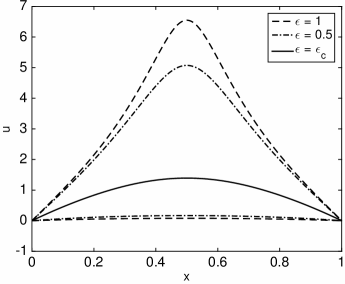
Figure 1. Bratu Problem. Slice at $y=0.5$, $0\leq x\leq 1$, of the upper and lower solutions computed with $\epsilon=1$ and $\epsilon=0.5$, together with the critical solution ($\epsilon=\epsilon_{c}$).

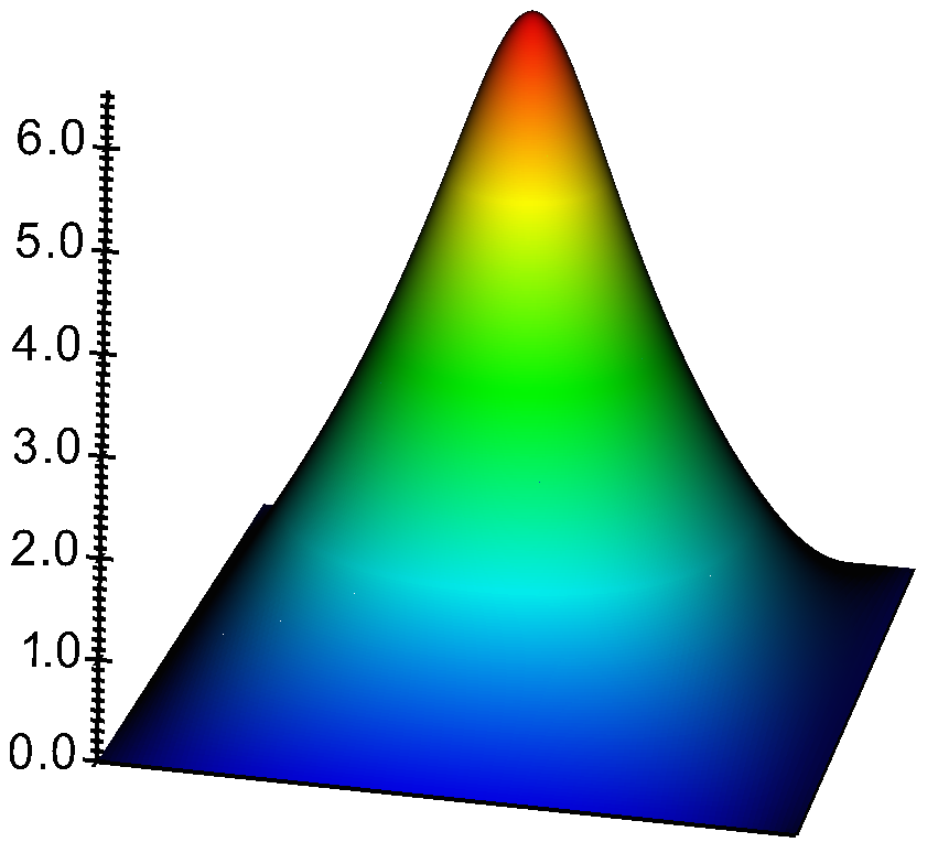
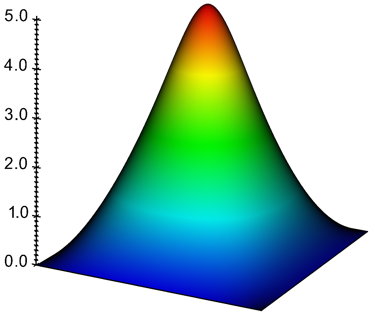
(a)	(b)

Figure 2. Bratu Problem. Upper solution computed with: (a) $\epsilon=1$; (b) $\epsilon=0.5$.

Example 6.1.

In this first example, we consider the Bratu problem

$$\epsilon\Delta u+{\rm e}^{u}=0\quad\mbox{ in }(0,1)^{2},$$

i.e., $f(u)={\rm e}^{u}+u$, subject to homogeneous Dirichlet boundary conditions on $\partial\Omega$. Writing $\lambda=\nicefrac{{1}}{{\epsilon}}$, we recall that there exists a critical parameter value $\lambda_{c}$ $(=1/\epsilon_{c})$, such that for $\lambda>\lambda_{c}$ $(\epsilon<\epsilon_{c})$ the problem has no solution, for $\lambda=\lambda_{c}$ $(\epsilon=\epsilon_{c})$ there exists exactly one solution, and for $\lambda<\lambda_{c}$ $(\epsilon>\epsilon_{c})$ there are two solutions. In the one–dimensional setting, an analytical expression for $\lambda_{c}$ is available, cf. [7, 17, 13]; for the two–dimensional case, calculations have revealed that $\lambda_{c}=6.808124423$ $(\epsilon_{c}=0.146883332)$ to 9 decimal places, see [17, 41, 40], and the references cited therein.

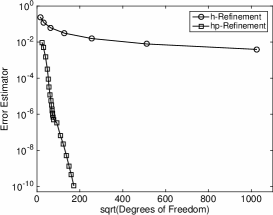
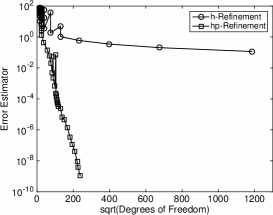
(a)	(b)
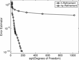
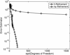
(c)	(d)
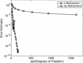
(e)

Figure 3. Bratu Problem. Comparison between $h$– and $hp$–refinement. (a) $\epsilon=1$ (lower solution); (b) $\epsilon=1$ (upper solution); (c) $\epsilon=\nicefrac{{1}}{{2}}$ (lower solution); (d) $\epsilon=\nicefrac{{1}}{{2}}$ (upper solution); (e) $\epsilon=\epsilon_{c}$ (critical solution);

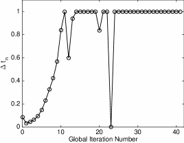
(a)	(b)
(c)	(d)
(e)	(f)

Figure 4. Bratu Problem. Damping parameter $\Delta t_{n}$. Left: $h$–refinement; right: $hp$–refinement. (a) & (b) $\epsilon=1$ (upper solution); (c) & (d) $\epsilon=\nicefrac{{1}}{{2}}$ (upper solution); (e) & (f) $\epsilon=\nicefrac{{1}}{{2}}$ (lower solution).

Following [40], we select the initial guess $u^{\text{\tiny\sf{DG}}}_{0}\in\mathcal{V}_{\text{\tiny\sf{DG}}}$ to be the $L^{2}$–projection of the function $u_{0}$ onto $\mathcal{V}_{\text{\tiny\sf{DG}}}$, where

$$u_{0}=a\sin(\pi x)\sin(\pi y)$$

and $a$ is a given amplitude. Noting that the maximum amplitude of the critical solution computed with $\epsilon=\epsilon_{c}$ is approximately $1.39$, selecting $a$ to be smaller/larger than this value leads to convergence to the so–called lower/upper solution, respectively. With this in mind we select $a=2$ when $\epsilon=\epsilon_{c}$, $a\in\{\nicefrac{{1}}{{10}},6\}$ for $\epsilon=1$, and $a\in\{1,4\}$ for $\epsilon=\nicefrac{{1}}{{2}}$; in the latter two cases the smaller value of $a$ is employed for the computation of the lower solution, while the larger value ensures convergence to the upper solution. In Figure 1 we plot a slice of each of the computed numerical solutions at $y=0.5$, $0\leq x\leq 1$. Here, we observe that the lower solutions tend to be rather flat in profile, while the upper solutions have a stronger peak in the middle of the computational domain, cf., also, Figure 2.

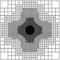
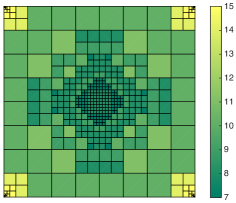
(a)	(b)
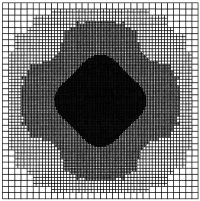
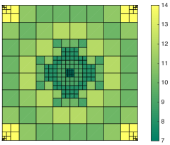
(c)	(d)
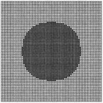
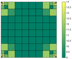
(e)	(f)

Figure 5. Bratu Problem. Computational meshes. Left: $h$–refinement; right: $hp$–refinement. (a) & (b) Upper solution computed with $\epsilon=1$; (c) & (d) Upper solution computed with $\epsilon=0.5$. (e) & (f) Critical solution.

In Figure 3 we demonstrate the performance of the proposed $hp$–adaptive NDG algorithm, cf. Algorithm 5.1, for the computation of the lower and upper solutions when $\epsilon=1$ and $\epsilon=\nicefrac{{1}}{{2}}$, as well as for the numerical approximation of the critical solution when $\epsilon=\epsilon_{c}$. In each case we plot the residual estimator ${\mathcal{E}}={\mathcal{E}}(u^{\text{\tiny\sf{DG}}}_{n},u^{\text{\tiny\sf{DG}}}_{n+1},{\bm{h}},{\bm{p}})$ versus the square root of the number of degrees of freedom in the finite element space $\mathcal{V}_{\text{\tiny\sf{DG}}}$, based on employing both $h$– and $hp$–refinement. For each parameter value we observe that the $hp$–refinement algorithm leads to an exponential decay of the residual estimator ${\mathcal{E}}$ as the finite element space $\mathcal{V}_{\text{\tiny\sf{DG}}}$ is adaptively enriched: on a linear-log plot, the convergence lines are roughly straight. Moreover, we observe the superiority of $hp$–refinement in comparison with a standard $h$–refinement algorithm, in the sense that the former refinement strategy leads to several orders of magnitude reduction in ${\mathcal{E}}$, for a given number of degrees of freedom, than the corresponding quantity computed exploiting mesh subdivision only.

In Figure 4 we plot the size of the Newton damping $\Delta t_{n}$ versus the global iteration number. In many of the cases considered here $\Delta t_{n}=1$ at all steps; for brevity, these results have been omitted. For the cases presented in Figure 4, we observe that initially the damping parameter slowly increases when we are far away from the solution; once the damping parameter is close to unity, the condition

$$\delta_{n,\Omega}^{2}\leq\Lambda\sum_{\kappa\in\mathcal{T}}{\eta_{\kappa,n}^{2}}$$

in Algorithm 5.1 becomes fulfilled in which case the finite element space $\mathcal{V}_{\text{\tiny\sf{DG}}}$ is adaptively enriched. In some cases, particularly at the early stages of the algorithm, refinement of $\mathcal{V}_{\text{\tiny\sf{DG}}}$ may then lead to a reduction in $\Delta t_{n}$, in which case further Newton steps are required before the next refinement can be undertaken. As the iterates approach the solution more closely, the size of the damping parameter typically remains approximately 1.

Finally, in Figure 5 we show the $h$– and $hp$–refined meshes generated for the numerical approximation of the upper solutions when $\epsilon=1$ and $\epsilon=\nicefrac{{1}}{{2}}$, as well as for the critical solution. Here we observe that when $h$–refinement is employed, the mesh is concentrated in the vicinity of the peak in the solution located at the centre of the computational domain, cf. Figures 1 & 2. In the $hp$–setting, we observe that while some mesh refinement has been undertaken in the centre of the domain $\Omega$, the corners of $\Omega$ have been significantly refined in order to resolve corner singularities typical for elliptic problems. Moreover, $p$–enrichement has been employed both in these corner regions, as well as in the vicinity of the peak in the computed solution. The corresponding meshes for the lower solutions are largely uniformly refined, due to the flat nature of the solution; for brevity, these have been omitted.

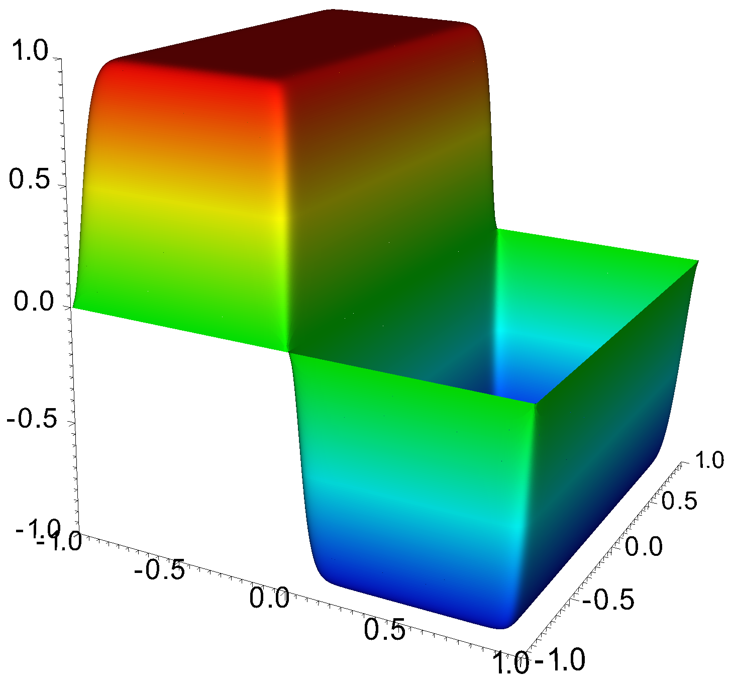
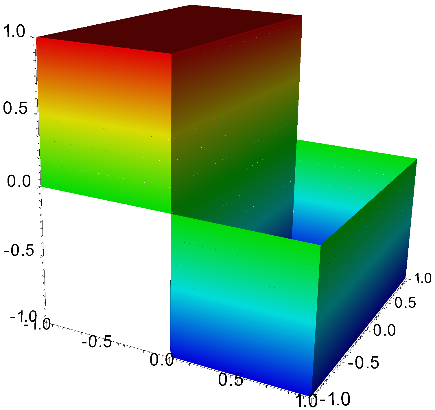
(a)	(b)

Figure 6. Ginzburg-Landau equation. Solution computed with: (a) $\epsilon=10^{-3}$; (b) $\epsilon=10^{-6}$.

Example 6.2.

In this example, we consider the Ginzburg-Landau equation given by

$$-\epsilon\Delta u+u=u(2-u^{2})\quad\mbox{ in }(-1,1)^{2},$$

subject to homogeneous Dirichlet boundary conditions on $\partial\Omega$. Following [5], we first note that $u\equiv 0$ is a solution; moreover, any solution $u$ appears in a pairwise fashion as $-u$. In the absence of boundary conditions, it is clear that $u=\pm 1$ are solutions of the Ginzburg-Landau equation. Thereby, in the presence of homogeneous Dirichlet boundary conditions, boundary layers will arise in the vicinity of $\partial\Omega$, whose width will be governed by the size of the diffusion coefficient $\epsilon$. Here, we select the initial guess $u^{\text{\tiny\sf{DG}}}_{0}\in\mathcal{V}_{\text{\tiny\sf{DG}}}$ to be the $L^{2}$–projection of the function $u_{0}(x,y)=-\mbox{sgn}(x)$ onto $\mathcal{V}_{\text{\tiny\sf{DG}}}$, subject to the enforcement of the boundary conditions. In this case the solution to the Ginzburg-Landau equation will possess not only boundary layers, but also an internal layer along $x=0$; in Figure 6 we plot the solution computed with both $\epsilon=10^{-3}$ and $\epsilon=10^{-6}$.

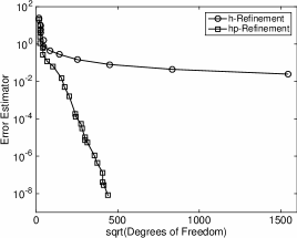
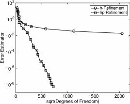
(a)	(b)
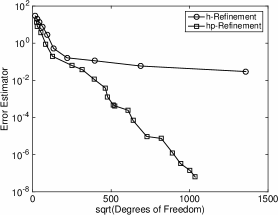
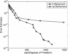
(c)	(d)

Figure 7. Ginzburg-Landau equation. Comparison between $h$– and $hp$–refinement. (a) $\epsilon=10^{-3}$; (b) $\epsilon=10^{-4}$; (c) $\epsilon=10^{-5}$; (d) $\epsilon=10^{-6}$.

In Figure 7 we demonstrate the performance of the proposed $hp$–adaptive NDG algorithm, cf. Algorithm 5.1, for the computation of the solution to the Ginzburg-Landau equation when $\epsilon=10^{-3},~{}10^{-4},~{}10^{-5},~{}10^{-6}$. In each case we plot the residual estimator ${\mathcal{E}}$ versus the square root of the number of degrees of freedom in the finite element space $\mathcal{V}_{\text{\tiny\sf{DG}}}$, based on employing both $h$– and $hp$–refinement. For each value of $\epsilon$ we again observe that the $hp$–refinement algorithm leads to an exponential decay of the residual estimator ${\mathcal{E}}$ as the finite element space $\mathcal{V}_{\text{\tiny\sf{DG}}}$ is adaptively enriched. Moreover, we again observe the superiority of exploiting $hp$–refinement in comparison with a standard $h$–refinement algorithm, in the sense that the former refinement strategy leads to several orders of magnitude reduction in ${\mathcal{E}}$, for a given number of degrees of freedom, than the corresponding quantity computed using $h$–refinement only. Furthermore, we note that as $\epsilon$ is reduced, additional $h$–enrichment of the computational mesh is required before $p$–refinement is employed. Indeed, for $\epsilon=10^{-6}$ we observe that there is an initial transient, before the $hp$–version convergence line becomes straight and exponential convergence is observed.

In Figure 8 we plot $\Delta t_{n}$ versus the global iteration number for $\epsilon=10^{-3}$; for the other values of $\epsilon$ considered here, the damping parameter was close to one on all of the meshes considered. As in the previous example, we again see an initial increase in $\Delta t_{n}$ as the adaptive Newton algorithm proceeds, before the underlying mesh is adaptively refined. Again, in the early stages of the algorithm, enrichment of $\mathcal{V}_{\text{\tiny\sf{DG}}}$ may lead to some additional damping, before $\Delta t_{n}$ tends to one.

Finally, in Figure 9 we plot the corresponding $h$– and $hp$–meshes generated for $\epsilon=10^{-3}$ and $\epsilon=10^{-6}$. Here, we clearly observe that the boundary and internal layers present in the analytical solution are refined by our adaptive mesh adaptation strategy; in particular, we emphasise that the NDG iterates converge to a solution which features the same topology as the initial guess, and, hence, does not switch between various attractors (corresponding to different solutions; see, e.g, [5]). In the $hp$–setting, we see that once the $h$–mesh has been sufficiently refined, then $p$–enrichment is employed.

(a)	(b)

Figure 8. Ginzburg-Landau equation. Damping parameter $\Delta t_{n}$ for $\epsilon=10^{-3}$. (a) $h$–refinement; (b) $hp$–refinement.

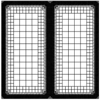
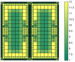
(a)	(b)
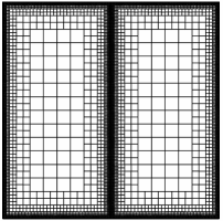
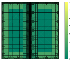
(c)	(d)

Figure 9. Ginzburg-Landau equation. Computational meshes. Left: $h$–refinement; right: $hp$–refinement. (a) & (b) $\epsilon=10^{-3}$; (c) & (d) $\epsilon=10^{-6}$.

7. Concluding remarks

In this article we have introduced the $hp$–version of the NDG scheme for the numerical approximation of second-order, singularly perturbed, semilinear elliptic boundary value problems. Here, the general approach is based on first linearising the underlying PDE problem on a continuous level, followed by subsequent discretisation of the resulting sequence of linear PDEs. For this latter task, in the current article we have exploited the $hp$–version of the interior penalty DG method. Furthermore, we have derived an $\epsilon$-robust a posteriori bound which takes into account both the linearisation and discretisation errors. On the basis of this residual estimate, we have designed and implemented an $hp$–adaptive refinement algorithm which automatically controls both of these sources of error; the practical performance of this strategy has been studied for a series of numerical test problems. Future work will be devoted to the extension of this technique to more general nonlinear PDE problems, as well as to problems in three dimensions.

References

- [1] P.R. Amestoy, I.S. Duff, J. Koster, and J.-Y. L’Excellent, A fully asynchronous multifrontal solver using distributed dynamic scheduling, SIAM J. Mat. Anal. Appl. 23 (2001), no. 1, 15–41.
- [2] P.R. Amestoy, I.S. Duff, and J.-Y. L’Excellent, Multifrontal parallel distributed symmetricand unsymmetric solvers, Comput. Methods Appl. Mech. Eng. 184 (2000), 501–520.
- [3] P.R. Amestoy, A. Guermouche, J.-Y. L’Excellent, and S. Pralet, Hybrid scheduling for the parallel solution of linear systems, Parallel Computing 32 (2006), no. 2, 136–156.
- [4] M. Amrein and T.P. Wihler, An adaptive Newton-method based on a dynamical systems approach, Commun. Nonlinear Sci. Numer. Simul. 19 (2014), no. 9, 2958–2973.
- [5] by same author, Fully adaptive Newton-Galerkin methods for semilinear elliptic partial differential equations, SIAM J. Sci. Comput. 37 (2015), no. 4, A1637–A1657.
- [6] D.N. Arnold, F. Brezzi, B. Cockburn, and L.D. Marini, Unified analysis of discontinuous Galerkin methods for elliptic problems, SIAM J. Numer. Anal. 39 (2001), 1749–1779.
- [7] U.M. Ascher, M.M. Mattheij, and R.D. Russell, Numerical solution of boundary value problems for ordinary differential equation, SIAM, Philadelphia, PA, 1995.
- [8] G. Barles and J. Burdeau, The Dirichlet problem for semilinear second-order degenerate elliptic equations and applications to stochastic exit time control problems, Comm. Partial Differential Equations 20 (1995), no. 1-2, 129–178.
- [9] A. Barone, F. Esposito, C.J. Magee, and A.C. Scott, Theory and applications of the Sine-Gordon equation, Riv. Nuovo Cim. 1 (1971), 227–267.
- [10] H. Berestycki and P.-L. Lions, Nonlinear scalar field equations. I. Existence of a ground state, Arch. Rational Mech. Anal. 82 (1983), no. 4, 313–345.
- [11] C. Bernardi, J. Dakroub, G. Mansour, and T. Sayah, A posteriori analysis of iterative algorithms for a nonlinear problem, J. Sci. Comput. 65 (2015), no. 2, 672–697.
- [12] A. Borisyuk, B. Ermentrout, A. Friedman, and D. Terman, Tutorials in mathematical biosciences. I, Lecture Notes in Mathematics, vol. 1860, Springer-Verlag, Berlin, 2005, Mathematical neuroscience, Mathematical Biosciences Subseries.
- [13] D. Calvetti and L. Reichel, Iterative methods for large continuation problems, J. Comput. Appl. Math. 123 (2000), 217–240.
- [14] R.S. Cantrell and C. Cosner, Spatial ecology via reaction-diffusion equations, Wiley Series in Mathematical and Computational Biology, John Wiley & Sons, Ltd., Chichester, 2003.
- [15] A.L. Chaillou and M. Suri, Computable error estimators for the approximation of nonlinear problems by linearized models, Comput. Methods Appl. Mech. Engrg. 196 (2006), no. 1-3, 210–224.
- [16] by same author, A posteriori estimation of the linearization error for strongly monotone nonlinear operators, J. Comput. Appl. Math. 205 (2007), no. 1, 72–87.
- [17] K.A. Cliffe, E. Hall, P. Houston, E.T. Phipps, and A.G. Salinger, Adaptivity and a posteriori error control for bifurcation problems I: The Bratu problem, Commun. Comput. Phys. 8 (2010), 845–865.
- [18] S. Congreve and P. Houston, Two-grid -version discontinuous Galerkin finite element methods for quasi-Newtonian fluid flows, Int. J. Numer. Anal. Model. 11 (2014), no. 3, 496–524.
- [19] S. Congreve, P. Houston, E. Süli, and T.P. Wihler, Discontinuous Galerkin finite element approximation of quasilinear elliptic boundary value problems II: strongly monotone quasi-Newtonian flows, IMA J. Numer. Anal. 33 (2013), no. 4, 1386–1415.
- [20] S. Congreve, P. Houston, and T.P. Wihler, Two-grid -version discontinuous Galerkin finite element methods for second-order quasilinear elliptic PDEs, J. Sci. Comput. 55 (2013), no. 2, 471–497.
- [21] S. Congreve and T.P. Wihler, An iterative finite element method for strongly monotone quasi-linear diffusion-reaction problems, in preparation, 2015.
- [22] L. Demkowicz, Computing with -adaptive finite elements. Vol. 1, Chapman & Hall/CRC Applied Mathematics and Nonlinear Science Series, Chapman & Hall/CRC, Boca Raton, FL, 2007, One and two dimensional elliptic and Maxwell problems.
- [23] P. Deuflhard, Newton methods for nonlinear problems, Springer Series in Computational Mathematics, vol. 35, Springer-Verlag, Berlin, 2004, Affine invariance and adaptive algorithms.
- [24] L. Edelstein-Keshet, Mathematical models in biology, Classics in Applied Mathematics, vol. 46, Society for Industrial and Applied Mathematics (SIAM), Philadelphia, PA, 2005, Reprint of the 1988 original.
- [25] T. Eibner and J. M. Melenk, An adaptive strategy for -FEM based on testing for analyticity, Comput. Mech. 39 (2007), no. 5, 575–595.
- [26] L. El Alaoui, A. Ern, and M. Vohralík, Guaranteed and robust a posteriori error estimates and balancing discretization and linearization errors for monotone nonlinear problems, Comput. Methods Appl. Mech. Engrg. 200 (2011), no. 37-40, 2782–2795.
- [27] T. Fankhauser, T.P. Wihler, and M. Wirz, The -adaptive FEM based on continuous Sobolev embeddings: isotropic refinements, Comp. Math. Appl. 67 (2014), no. 4, 854–868.
- [28] E.M. Garau, P. Morin, and C. Zuppa, Convergence of an adaptive Kačanov FEM for quasi-linear problems, Appl. Numer. Math. 61 (2011), no. 4, 512–529.
- [29] J.D. Gibbon, I.N. James, and I.M. Moroz, The Sine-Gordon equation as a model for a rapidly rotating baroclinic fluid, Phys. Script. 20 (1979), 402–408.
- [30] W. Han, A posteriori error analysis for linearization of nonlinear elliptic problems and their discretizations, Math. Method Appl. Sci. 17 (1994), no. 7, 487–508.
- [31] P. Houston, D. Schötzau, and T.P. Wihler, An -adaptive mixed discontinuous Galerkin FEM for nearly incompressible linear elasticity, Comput. Methods Appl. Mech. Engrg. 195 (2006), no. 25-28, 3224–3246.
- [32] by same author, Energy norm a posteriori error estimation of -adaptive discontinuous Galerkin methods for elliptic problems, Math. Models Methods Appl. Sci. 17 (2007), no. 1, 33–62.
- [33] P. Houston and E. Süli, Adaptive finite element approximation of hyperbolic problems, Error Estimation and Adaptive Discretization Methods in Computational Fluid Dynamics. Lect. Notes Comput. Sci. Engrg. (T. Barth and H. Deconinck, eds.), vol. 25, Springer, 2002, pp. 269–344.
- [34] by same author, A note on the design of -adaptive finite element methods for elliptic partial differential equations, Comput. Methods Appl. Mech. Engrg. 194 (2005), no. 2-5, 229–243.
- [35] P. Houston, E. Süli, and T.P. Wihler, A posteriori error analysis of -version discontinuous Galerkin finite-element methods for second-order quasi-linear elliptic PDEs, IMA J. Numer. Anal. 28 (2008), no. 2, 245–273.
- [36] P. Houston and T.P. Wihler, Adaptive energy minimisation for -finite element methods, Comput. Math. Appl. 71 (2016), no. 4, 977 – 990.
- [37] O.A. Karakashian and F. Pascal, A posteriori error estimation for a discontinuous Galerkin approximation of second order elliptic problems, SIAM J. Numer. Anal. 41 (2003), 2374–2399.
- [38] M. Karkulik and J.M. Melenk, Local high-order regularization and applications to -methods, Comp. Math. Appl. 70 (2015), no. 7, 1606–1639.
- [39] W.F. Mitchell and M.A. McClain, A comparison of -adaptive strategies for elliptic partial differential equations, ACM. Transactions on Mathematical Software 41 (2014), no. 1, 2:1–39.
- [40] A. Mohsen, A simple solution of the Bratu problem, Comput. Math. Appl. 67 (2014), 26–33.
- [41] A. Mohsen, L.F. Sedeek, and S.A. Mohamed, New smoother to enhance multigrid–based methods for Bratu problem, Appl. Math. Comput. 204 (2008), 325–339.
- [42] W.-M. Ni, The mathematics of diffusion, CBMS-NSF Regional Conference Series in Applied Mathematics, vol. 82, Society for Industrial and Applied Mathematics (SIAM), Philadelphia, PA, 2011.
- [43] A. Okubo and S.A. Levin, Diffusion and ecological problems: modern perspectives, second ed., Interdisciplinary Applied Mathematics, vol. 14, Springer-Verlag, New York, 2001.
- [44] H.R. Schneebeli and T.P. Wihler, The Newton-Raphson method and adaptive ODE solvers, Fractals. Complex Geometry, Patterns, and Scaling in Nature and Society 19 (2011), no. 1, 87–99.
- [45] D. Schötzau, C. Schwab, and A. Toselli, Mixed -DGFEM for incompressible flows, SIAM J. Numer. Anal. 40 (2002), no. 6, 2171–2194 (electronic) (2003).
- [46] P. Solin, K. Segeth, and I. Dolezel, Higher-order finite element methods, Studies in advanced mathematics, Chapman & Hall/CRC, Boca Raton, London, 2004.
- [47] B. Stamm and T.P. Wihler, -Optimal discontinuous Galerkin methods for linear elliptic problems, Math. Comp. 79 (2010), no. 272, 2117–2133.
- [48] W.A. Strauss, Existence of solitary waves in higher dimensions, Comm. Math. Phys. 55 (1977), no. 2, 149–162.
- [49] R. Verfürth, Robust a posteriori error estimators for a singularly perturbed reaction-diffusion equation, Numer. Math. 78 (1998), no. 3, 479–493.
- [50] T.P. Wihler, P. Frauenfelder, and C. Schwab, Exponential convergence of the -DGFEM for diffusion problems, Comp. Math. Appl. 46 (2003), no. 1, 183–205.
- [51] L. Zhu, S. Giani, P. Houston, and D. Schötzau, Energy norm a posteriori error estimation for -adaptive discontinuous Galerkin methods for elliptic problems in three dimensions, Math. Models Methods Appl. Sci. 21 (2011), no. 2, 267–306.
- [52] L. Zhu and D. Schötzau, A robust a posteriori error estimate for -adaptive DG methods for convection-diffusion equations, IMA J. Numer. Anal. 31 (2011), 971–1005.