Elastically-mediated interactions between grain boundaries and precipitates in two-phase coherent solids

Abstract

We investigate analytically and numerically the interaction between grain boundaries and second phase precipitates in two-phase coherent solids in the presence of misfit strain. Our numerical study uses amplitude equations that describe the interaction of composition and stress [R. Spatschek and A. Karma, Phys. Rev. B 81, 214201 (2010)] and free-energies corresponding to two-dimensional hexagonal and three-dimensional BCC crystal structures that exhibit isotropic and anisotropic elastic properties, respectively. We consider two experimentally motivated geometries where (i) a lamellar precipitate nucleates along a planar grain boundary that is centered inside the precipitate, and (ii) a circular precipitate nucleates inside a grain at a finite distance to an initially planar grain boundary. For the first geometry, we find that the grain boundary becomes morphologically unstable due to the combination of long-range elastic interaction between the grain boundary and compositional domain boundaries, and shear-coupled grain boundary motion. We characterize this instability analytically by extending the linear stability analysis carried out recently [P.-A. Geslin, Y.-C. Xu, and A. Karma, Phys. Rev. Lett. 114, 105501 (2015)] to the more general case of elastic anisotropy. The analysis predicts that elastic anisotropy hinders but does not suppress the instability. Simulations also reveal that, in a well-developed non-linear regime, this instability can lead to the break-up of low-angle grain boundaries when the misfit strain exceeds a threshold that depends on the grain boundary misorientation. For the second geometry, simulations show that the elastic interaction between an initially planar grain boundary and an adjacent circular precipitate causes the precipitate to migrate to and anchor at the grain boundary.

I Introduction

Phase separation into domain structures of distinct chemical compositions occurs in a wide range of technological materials. Nucleation and growth of second phase precipitates inside the matrix of a primary phase is commonly used as a strengthening mechanism of structural materials Porter and Easterling (1992). Domain structures also commonly form by spinodal decomposition into two phases, which has been widely investigated in various contexts Cahn (1961); Ramanarayan and Abinandanan (2003); Haataja and Léonard (2004); Haataja et al. (2005); Hu and Chen (2004); Tang et al. (2010); Hoyt and Haataja (2011); Lu et al. (2012); Tang and Karma (2012); Tao et al. (2012); Wang et al. (2013). Due to the dependence of the crystal lattice spacing on composition, domain formation typically generates a misfit strain that can be large in some cases, e.g. several percent in phase-separating lithium iron phosphate battery electrode materials Tang et al. (2010).

The effect of a coherency stress has been investigated theoretically in the context of both single-crystalline and polycrystalline materials. In single-crystalline materials, Cahn demonstrated that coherency stress hinders spinodal decomposition, requiring a larger chemical driving force than in the absence of misfit to generate phase-separation inside a bulk material Cahn (1961). A recent extension of this analysis showed that stress relaxation near a free surface can lead to spinodal decomposition for smaller chemical driving forces than inside a bulk material, with compositional domain formation confined at the surface Tang and Karma (2012). In polycrystalline materials, numerical simulations have been used to investigate the interaction between compositional domain boundaries (DBs) and dislocations using continuum dislocation-based models Haataja and Léonard (2004); Haataja et al. (2005); Hoyt and Haataja (2011) phase-field approaches Hu and Chen (2004). More recently, the interaction between DBs and grain boundaries (GBs) has also been investigated using phase-field-crystal (PFC) simulations Tao et al. (2012); Wang et al. (2013), and amplitude equations derived from the PFC framework Elder and Huang (2010). Those studies have shown that dislocations generically migrate to DBs to relax the coherency stress thereby strongly impacting microstructural evolution and domain coarsening behavior Haataja et al. (2005); Tao et al. (2012); Wang et al. (2013).

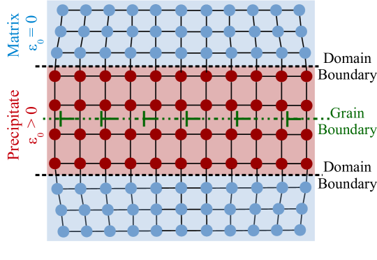
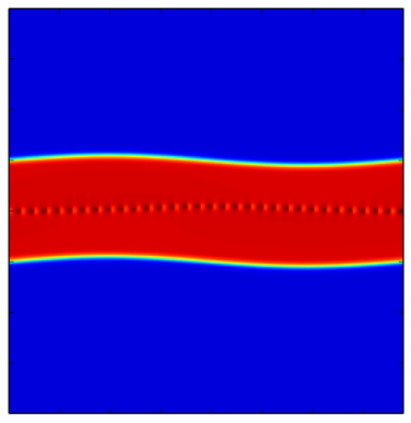
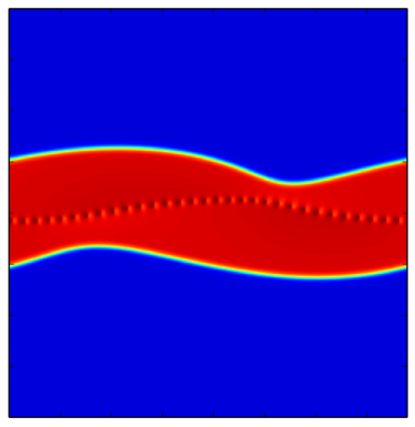
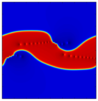
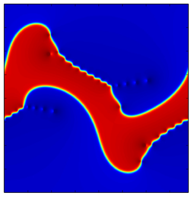
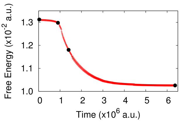
Figure 1: (a) Scheme representing the configuration consisting of a misfitting lamellar precipitate centered on a low angle grain boundary. (b-e) Color plots of the composition field $c$ at times of (b) $0.03\times 10^{6}$, (c) $0.9\times 10^{6}$, (d) $1.4\times 10^{6}$ and (e) $6.37\times 10^{6}$ illustrating the destabilization of a low-angle GB ($\theta=7.2\mathrm{\SIUnitSymbolDegree}$) due to the presence of a misfitting precipitate (red domain) computed with the amplitude equation model for hexagonal symmetry and with a misfit eigenstrain $\varepsilon_{0}=0.043$. Dislocations are visible because the composition profile is altered in their vicinity. The system size is $249.6a\times 361.6a$ ($a$ being the lattice spacing) and periodic boundary conditions are used in both $x$ and $y$ directions. Only part of the system is shown in the $y$ direction. (f) Time evolution of the free energy, showing the relaxation of the system towards an equilibrium state. Black dots locate the snapshots of panels (b-e).

Experimental observations also testify of strong interactions between GBs and precipitates. For example, in Ni-Al superalloys, $\gamma^{\prime}$ precipitates in the vicinity of GBs have been shown to be responsible for GB serration, leading to improved mechanical properties at high temperature Koul and Gessinger (1983); Mitchell et al. (2009). In addition, in steel and Ti-based alloys submitted to thermo-mechanical treatments, acicular Widmanstätten precipitates, are observed to grow from the GBs in a direction normal to the GB plane Teixeira et al. (2006); Cheng et al. (2010). While the stationary growth kinetics of these structures have been recently clarified Cottura et al. (2014), the initial stage of growth that involves the nucleation of precipitates along the GBs is not understood. In both examples, elastic interactions between GBs and precipitates might play a central role in the development of these microstructures. However, these interactions remain largely unexplored due to the complexity of the problem at hand that involves elastic interactions, grain boundary migration, and solute diffusion.

In a recent study Geslin et al. (2015), we provided further insight into the complex interaction between crystal defects and precipitates by investigating the situation in which a planar GB is centered inside a misfitting lamellar precipitate (see Fig. 1.a). This choice of geometry is physically motivated by the fact that dislocations act as preferred sites of nucleation Cahn (1957); Hu and Chen (2001); Léonard and Haataja (2005). Hence GBs naturally seed the formation of lamellar precipitates of this approximate geometry Ramanarayan and Abinandanan (2003); Zhao and Notis (1998). Using a nonlinear elastic model Geslin et al. (2014); Geslin (2013) and amplitude equations (AE) that describe the interaction between composition and stress Spatschek and Karma (2010), we showed that this configuration is morphologically unstable. This instability is illustrated in Fig. 1.b-e that shows a sequence of GB and precipitate configurations obtained by AE simulations Geslin et al. (2015). Furthermore, we carried out a linear stability analysis to predict the onset and wavelength of this instability. The starting point of this analysis is a free-boundary problem governing the coupled evolution of DBs and GBs, which corresponds to the sharp-interface limit of the AE model (i.e. the limit where the DBs and GB can be treated as sharp boundaries). The physical mechanism of this instability can be qualitatively understood by considering a small initial sinusoidal perturbation of DBs of wavelength $\Lambda=2\pi/k$. In the case of isotropic elasticity, the elastic energy is unchanged by this perturbation because the Bitter-Crum theorem Bitter (1931); Fratzl et al. (1999) implies that this energy is independent of the shape of the precipitate and only depends on its volume, which remains constant. In the absence of a GB inside the precipitate, the DB is stable because the perturbation of its interface increases the total DB surface, therefore increasing the total energy of the system. In contrast, with a GB present, the elastic energy can be decreased by the relaxation of the shear stress, induced by the DB perturbation, along the GB plane via shear-coupled GB motion Cahn and Taylor (2004); Cahn et al. (2006); Ivanov and Mishin (2008); Gorkaya et al. (2009); Olmsted et al. (2009); Molodov et al. (2011); Trautt et al. (2012); Karma et al. (2012); Rajabzadeh et al. (2014); Rupert et al. (2009); Sharon et al. (2011); Winning et al. (2010); Lim et al. (2012). Namely, the GB can move normal to its plane under an applied shear stress. This behavior referred as coupling is characterized by the relation

$$v_{\parallel}=\beta v_{n}$$ (1)

between the velocity $v_{n}$ of the GB normal to the GB plane and the rate $v_{\parallel}$ of parallel grain translation. In the case of pure coupling, the coefficient $\beta$ is a geometrical factor depending only on GB bicrystallography with the coupling factor $\beta$ obtained from the geometrical relation between dislocation glide motion and crystal lattice translation Sutton and Balluffi (1995); Cahn and Taylor (2004); Cahn et al. (2006). Computations and experiments have shown that a wide range of both low- and high-angle GBs display shear-coupled motion Cahn et al. (2006); Ivanov and Mishin (2008); Gorkaya et al. (2009); Olmsted et al. (2009); Molodov et al. (2011); Trautt et al. (2012); Karma et al. (2012); Rajabzadeh et al. (2014). Furthermore, GB coupling has been found to influence significantly the coarsening behavior of polycrystalline materials in more complex multi-grain geometries where GBs form a complex network Rupert et al. (2009); Sharon et al. (2011); Wu and Voorhees (2012); Trautt et al. (2012); Adland et al. (2013a).

Our recent study Geslin et al. (2015) has highlighted the fundamental role of shear-coupled GB motion in the interaction between GBs and precipitates. However, this study only considered a limited range of misfit strain and GB misorientation and was limited to isotropic elasticity and a lamellar precipitate geometry. Materials forming second phase precipitates are often elastically anisotropic. This anisotropy is known to influence the shape of misfitting precipitates by inducing DBs to align along preferred crystallographic directions to minimize the elastic energy Khachaturyan (2013). Moreover, it also influences the elastic interaction between GBs and precipitates. In particular, the Bitter-Crum theorem Bitter (1931); Fratzl et al. (1999) invoked above to explain the destabilization of the GB for isotropic elasticity no longer applies within elastic anisotropy. In this case, deformation of the precipitate shape increases the elastic energy and can hinder or even potentially suppress the GB morphological instability. Furthermore, in several important experimental situations, precipitates interacting with GBs have a circular or cuboid geometry if nucleation occurs away from the GB at multiple sites, e.g. $\gamma^{\prime}$ precipitates in Ni-Al superalloys. It is unclear how in those situations, closed-shape precipitates interact with GBs and what role shear-coupled motion plays in this interaction.

In this paper, we extend the study of Ref. [Geslin et al., 2015] to investigate the interaction between GBs and precipitates of different shapes with and without elastic anisotropy. We first focus on the lamellar precipitate geometry and extend the linear stability analysis of Ref. [Geslin et al., 2015] to anisotropic elastic behavior. This extension is conceptually straightforward even though the anisotropy makes the analysis more lengthy. The analysis predicts that elastic anisotropy hinders the instability, because of the energetic cost of deforming the lamellar precipitate, but does not suppress it. We test this prediction using the same AE approach as in Refs. [Spatschek and Karma, 2010] and [Geslin et al., 2015], albeit with a free-energy form that favors an elastically anisotropic 3D body-centered-cubic (BCC) structure. The simulation results are in good quantitative agreement with the predictions of the linear stability analysis. For a free-energy form that favors an elastically isotropic two-dimensional (2D) hexagonal structure, we investigate the nonlinear development of the instability over a wider range of misfit strain and misorientation than in Ref. [Geslin et al., 2015]. Simulations yield the novel insight that, in a well-developed non-linear regime, this instability can lead to the break-up of low-angle GBs when the misfit strain exceeds a threshold that depends on misorientation. Next, we investigate in 2D the interactions between a circular precipitate and a grain boundary. We find that a similar elastic interaction mediated by shear-coupled GB motion leads to the attraction of the precipitate to the GB. The GB and precipitate shape are simultaneously deformed in this process that can also lead to GB break-up for large enough misfit strain.

Some properties of the amplitude equations (AE) approach relevant to the present study are worth pointing out. AE models can be generally derived from the phase-field-crystal (PFC) model Elder et al. (2002); Elder and Grant (2004); Berry et al. (2006) via a multiscale expansion Goldenfeld et al. (2005); Athreya et al. (2006); Spatschek and Karma (2010). This expansion is formally valid in the limit where the correlation length of liquid density fluctuations (which sets of the width of the spatially diffuse solid-liquid interface at the melting point of a pure material) is much larger than the lattice spacing. AE models can also be derived in the spirit of Ginzburg-Landau expansions of a free-energy functional in terms of complex density wave amplitudes from symmetry considerations (see Ref. [Wu et al., 2015] and earlier references therein for a comparison of both approaches for solid-liquid interface properties). The latter approach provides more flexibility to formulate AE models with a minimal set of model parameters that can be related to material parameters. For this reason, it was used in Ref. [Spatschek and Karma, 2010] to derive the set of AEs that describes the interaction of composition, stress, and crystal defects. The parameters of this AE model, used here and in our previous study Geslin et al. (2015), are uniquely fixed by the DB energy $\gamma$, the misfit strain $\varepsilon_{0}$, linear elastic properties, and the dislocation core size that is proportional to the correlation length. Like PFC, the AE method describes dislocation glide, therefore reproducing salient features of GB shear-coupled motion for a wide range of GB bi-crystallography Trautt et al. (2012), and also dislocation climb. Since PFC and AE models do not track explicitly the vacancy concentration, the climb kinetics is modeled only heuristically. However, the incorporation of dislocation climb is important in that it provides an additional mechanism to relax the total free-energy as is apparent in Fig. 1 where the final equilibrium configuration was attained by a combination of both dislocation glide and climb. Finally, as shown in Ref. [Spatschek and Karma, 2010], the AE model can only describe GBs over a limited range of misorientation due to the choice of a fixed reference set of crystal axes to represent the crystal density waves. However, this limitation is not too stringent as the method is able to describe both low-angle GBs with separate dislocations and higher angle ones with overlapping dislocation cores.

This paper is organized as follows. We start by introducing in section II the AE model for both hexagonal (isotropic elasticity) and BCC ordering (anisotropic elasticity). The following section III is dedicated to generalizing the linear stability analysis to the case of anisotropic elasticity. In particular, we show that the introduction of elastic anisotropy inhibits the instability by reducing the growth rate and decreasing the range of unstable wavelengths. Next, in section IV, we investigate more closely the nonlinear regime of instability for isotropic elasticity, showing that a sufficiently large misfit strain can lead to GB break-up. Finally, in section V, we investigate the interactions between circular precipitates and a GB, showing that similar elastic interaction leads to the attraction of the precipitate to the GB and can also lead to GB break-up.

II Amplitude-Equation model

II.1 Free-energies

In the present study, we used the AE approach developed by Spatschek and Karma Spatschek and Karma (2010), which provides a general methodology for modeling the interaction of composition and stress Spatschek and Karma (2010). In this AE framework, the atomic density field is expanded as a sum of crystal density waves

$$n(\vec{r},t)=n_{0}+\delta n_{s}\sum_{n=1}^{N/2}\left(A_{n}e^{i\vec{k}_{n}\cdot\vec{r}}+A_{n}^{*}e^{-i\vec{k}_{n}\cdot\vec{r}}\right),$$ (2)

where $\pm\vec{k}_{n}$ ($1\leq n\leq N/2$) correspond to the $N$ principal reciprocal lattice vectors (RLVs) of equal magnitude $|\vec{k}_{n}|=q_{0}=2\pi/a$, where $a$ is the lattice spacing, $n_{0}$ is a reference average value of this field, and $\delta n_{s}$ is a scale factor that can be adjusted to match arbitrary values of solid density wave amplitudes. The amplitudes have a constant value $|A_{n}|=A_{s}$ in a perfect crystal, and decrease to low values in the atomically disordered core region of dislocations, which is similar to the liquid phase where the amplitudes vanish.

The total free-energy of the system is given by the functional:

$$F=\int dVf_{c}+\int dVf_{el},$$ (3)

where the chemical and elastic parts of the free-energy density are defined respectively by

$$f_{c}=\frac{K}{2}|\nabla c|^{2}+f_{dw}(c)$$ (4)

and

$$f_{el}=F_{0}\bigg{[} \xi_{d}^{2}\sum_{n=1}^{N}|(\Box_{n}+i\varepsilon_{0}q_{0}c)A_{n}|^{2}$$

$$+f_{b}(\{A_{n}\},\{A_{n}^{*}\})\bigg{]},$$ (5)

where the “box operator” is defined by $\Box_{n}=\hat{k}_{n}\cdot{\nabla}-\frac{i}{2q_{0}}{\nabla}^{2}$. This elastic free energy density represents the energy cost of an arbitrary perturbation of the atomic density field associated with linear elastic deformations and crystal defects (nonlinear deformations) such as dislocations or grain boundaries.

The free-energy cost of defects is captured by the box operator that is introduced to insure that the elastic part of the free-energy is rotationally invariant Spatschek and Karma (2010). In addition, the operator $i\varepsilon_{0}q_{0}c$, accounts for the influence of the compositional field on the lattice spacing through the misfit strain $\varepsilon_{0}$, where we assume a linear relationship between strain and concentration (Vegard’s law). The parameter $\xi_{d}$ is a dimensionless coefficient that is proportional to the width of the solid-liquid interface at the melting point and also sets the scale of the dislocation core.

As in our previous study Geslin et al. (2015), we use a version of the AE model where the bulk chemical free-energy density has a standard double-well Cahn-Hilliard-like contribution Cahn and Hilliard (1959) $f_{dw}(c)$ that favors phase separation into two solid phases of distinct chemical compositions Geslin et al. (2015).

The bulk chemical free-energy density has the double-well form

$$f_{dw}(c)=g(c-c_{0}^{-})^{2}(c-c_{0}^{+})^{2},$$ (6)

where the minima ($c_{0}^{\pm}$) represent the equilibrium concentrations in the composition domains in the absence of stress and the expressions

$$g= \frac{12\gamma}{w_{i}(c_{0}^{+}-c_{0}^{-})^{4}}$$ (7)

$$K= \frac{3w_{i}\gamma}{2(c_{0}^{+}-c_{0}^{-})^{2}},$$ (8)

relate the parameters $g$ and $K$ to the width $w_{i}$ and excess free-energy $\gamma$ of the spatially diffuse boundary between those domains.

The RLVs and the bulk part of the elastic energy density, $f_{b}(\{A_{n}\},\{A_{n}^{*}\})$, can be chosen to stabilize different crystalline structures Wu et al. (2010); Greenwood et al. (2011); Tóth et al. (2010). In this study, we consider the 2D hexagonal lattice described by $N=6$ RLVs $\vec{k}_{n}=\pm q_{0}\hat{k}_{n}$ where

$$\hat{k}_{1}=\left(-\frac{\sqrt{3}}{2},-\frac{1}{2}\right),\enskip\hat{k}_{2}=\left(0,1\right),\enskip\hat{k}_{3}=\left(\frac{\sqrt{3}}{2},-\frac{1}{2}\right)$$

and

$$f_{b}^{HEX}(\{A_{n}\},\{A_{n}^{*}\})=\frac{1}{6}\sum_{n=1}^{3}A_{n}A_{n}^{*}+\frac{1}{2}(A_{1}A_{2}A_{3}+A_{1}^{*}A_{2}^{*}A_{3}^{*})+\frac{1}{15}\left(\sum_{n=1}^{3}A_{n}A_{n}^{*}\right)^{2}-\frac{1}{30}\sum_{n=1}^{3}|A_{n}|^{4},$$ (9)

which reproduce isotropic elasticity for small deformations Spatschek and Karma (2010). To investigate the effect of anisotropic elasticity, we also consider BCC ordering described by $N=12$ RLVs $\vec{k}_{n}=\pm q_{0}\hat{k}_{n}$ where:

$$\hat{k}_{1}=\frac{1}{\sqrt{2}}(1,1,0),\quad\hat{k}_{2}=\frac{1}{\sqrt{2}}(1,0,1),\quad\hat{k}_{3}=\frac{1}{\sqrt{2}}(0,1,1),\quad\hat{k}_{4}=\frac{1}{\sqrt{2}}(1,-1,0),\quad\hat{k}_{5}=\frac{1}{\sqrt{2}}(1,0,-1),\quad\hat{k}_{6}=\frac{1}{\sqrt{2}}(0,1,-1),$$

and the function Spatschek and Karma (2010)

$$f_{b}^{BCC}(\{A_{n}\},\{A_{n}^{*}\})= \frac{1}{12}\sum_{n=1}^{6}A_{n}A_{n}^{*}++\frac{1}{90}\Bigg{\{}\bigg{(}\sum_{n=1}^{6}A_{n}A_{n}^{*}\bigg{)}^{2}-\frac{1}{2}\sum_{n=1}^{6}|A_{n}|^{4}+2A_{1}^{*}A_{2}A_{4}^{*}A_{5}+2A_{1}A_{2}A_{4}^{*}A_{5}^{*}$$

$$+2A_{1}^{*}A_{3}A_{4}A_{6}+2A_{1}A_{3}^{*}A_{4}^{*}A_{6}^{*}+2A_{2}A_{3}^{*}A_{5}^{*}A_{6}+2A_{2}^{*}A_{3}A_{5}A_{6}^{*}\Bigg{\}}$$

$$-\frac{1}{8}\Big{\{}A_{2}A_{3}^{*}A_{4}^{*}+A_{2}A_{3}^{*}A_{4}+A_{1}A_{3}^{*}A_{5}^{*}+A_{1}^{*}A_{3}A_{5}$$

$$+A_{1}A_{2}^{*}A_{6}^{*}+A_{1}^{*}A_{2}A_{6}+A_{4}^{*}A_{5}A_{6}^{*}+A_{4}A_{5}^{*}A_{6}\Big{\}}.$$ (10)

The effect of the anisotropic elasticity of the BCC structure on the precipitate morphology is illustrated in Figure 2. An initially circular precipitate of radius $R=40.5a$ and eigenstrain $\varepsilon_{0}=0.043$ (Figure 2.a) evolves into a square with rounded corners (Figure 2.b). Even though this morphology increases the surface energy, it is the equilibrium state of the system because of the drop of elastic energy due to anisotropic elasticity effects Khachaturyan (2013).

Figure 2: An initially circular precipitate of radius $R=40.5a$ and eigenstrain $\varepsilon_{0}=0.043$ (a) relaxes to a square shape with rounded corners (b) due to the anisotropic elasticity in the BCC AE model.

II.2 Determination of model parameters

The free-energies of the AE model depend on eight parameters $c_{0}^{\pm}$, $g$, $K$, $q_{0}$, $\xi_{d}$, $\varepsilon_{0}$, and $F_{0}$. Their value can be generally determined uniquely in terms of material parameters as follows. The phase diagram determines $c_{0}^{\pm}$, the lattice spacing $a$ determines $q_{0}=2\pi/a$, the compositional domain width $w_{i}$ and the interface free-energy $\gamma$ determine $g$ and $K$ via Eqs. (7) and (8). The misfit strain $\varepsilon_{0}$ is a known material parameter and the microscopic length $\sim\xi_{d}$ can be in principle estimated by matching the dislocation core size to experimental measurement or the results of atomistic simulations; for simplicity here we choose $\xi_{d}q_{0}=1$. In addition, $F_{0}$ can be related to elastic constants of the material using relations derived in Ref. [Spatschek and Karma, 2010]. In the case of the elastically isotropic hexagonal model, the elastic constants are $C_{11}=C_{22}=\lambda+2G=\frac{9}{4}F_{0}A_{s}^{2}\xi_{d}^{2}q_{0}^{2}$ and $C_{12}=C_{44}=\lambda=\frac{3}{4}F_{0}A_{s}^{2}\xi_{d}^{2}q_{0}^{2}$, yielding a Poisson ratio $\nu=\lambda/[2(\lambda+G)]=0.25$ ($\lambda$ and $G$ denote the Lamé coefficients). For the elastically anisotropic BCC model, $C_{11}=C_{22}=C_{33}=2F_{0}A_{s}^{2}\xi_{d}^{2}q_{0}^{2}$ and $C_{12}=C_{23}=C_{44}=F_{0}A_{s}^{2}\xi_{d}^{2}q_{0}^{2}$. In these definition, the coefficient $A_{s}$ denotes the amplitude of solid density waves in a perfect crystal and can be expressed as

$$A_{s}=\frac{3+\sqrt{1-Z\varepsilon_{0}^{2}c_{0}^{2}\xi_{d}^{2}q_{0}^{2}}}{4},$$ (11)

where $Z=48$ ($Z=96$) for the hexagonal (BCC) lattice. Let us notice that for small values of $\varepsilon_{0}$, $A_{s}$ depends weakly on composition $c_{0}$ via a shift of the lattice constant induced by the misfit strain.

In this study, simulations are performed for a generic set of material parameters similar to the one used to model phase separation in Li-ion battery materials Tang and Karma (2012). In particular, we choose $c_{0}^{-}=0.05$, $c_{0}^{+}=0.95$, $\gamma=$0.2\text{\,}\mathrm{J}\mathrm{/}\mathrm{m}^{2}$$, and $w_{i}=$2\text{\,}\mathrm{n}\mathrm{m}$$, yielding $g=$1.8\times 10^{9}\text{\,}\mathrm{J}\mathrm{/}\mathrm{m}^{3}$$ and $K=$7.4\times 10^{-10}\text{\,}\mathrm{J}\mathrm{/}\mathrm{m}$$ using Eqs. (7) and (8). In addition, we take $a=$0.5\text{\,}\mathrm{n}\mathrm{m}$$, $\xi_{d}q_{0}=1$, and $G=C_{44}=$39\text{\,}\mathrm{G}\mathrm{P}\mathrm{a}$$, yielding $F_{0}=4G/(3A_{s}^{2}\xi_{d}^{2}q_{0}^{2})=$5.2\times 10^{10}\text{\,}\mathrm{J}\mathrm{/}\mathrm{m}^{3}$$ for the hexagonal lattice and $F_{0}=C_{44}/(A_{s}^{2}\xi_{d}^{2}q_{0}^{2})=$3.9\times 10^{10}\text{\,}\mathrm{J}\mathrm{/}\mathrm{m}^{3}$$ for the BCC lattice where $A_{s}\approx 1$ is used in those relations to compute $F_{0}$. This is equivalent to neglecting the dependence of $A_{s}$ on $c_{0}$ in Eq. (11), which is negligible for small misfit strain. In the following, the simulations used to test the predictions of the linear stability analysis are carried out with $\varepsilon_{0}=0.043$ for both the hexagonal and BCC models. Additional simulations are carried out for various values of $\varepsilon_{0}$ to explore the influence of the misfit strain on the equilibrium state of the microstructure. Mathematically, the AE model is only valid for small misorientations between grains. However, it has been shown Spatschek and Karma (2010) that the predictions of the GB energy from AE remain valid over roughly half the complete range allowed by the full crystal symmetry. Therefore, the limitations of the AE model on grain rotations does not influence significantly the results obtained for misorientations below $30\mathrm{\SIUnitSymbolDegree}$ investigated in this article.

II.3 Dynamical equations

The concentration field $c$ is assumed to follow a conserved dynamics

$$\frac{\partial c}{\partial t}=M\nabla^{2}\frac{\delta F}{\delta c}.$$ (12)

where the mobility $M=Df_{dw}^{\prime\prime}(c_{0}^{\pm})$ is chosen such that Fickian diffusion is recovered for vanishing stresses and composition close to the equilibrium values $c_{0}^{\pm}$. We note here that for finite misfit, the equilibrium concentrations in the low ($c^{-}$) and high ($c^{+}$) concentration domains are slightly shifted from their equilibrium values $c_{0}^{\pm}$ as described further in the paper, but this shift has a negligible effect on the effective value of the mobility.

On the other hand, The amplitudes $A_{n}$ are evolved using a formulation of non-conserved dynamics introduced previously in the context of the PFC model Stefanovic et al. (2006, 2009) to relax the elastic field rapidly over the entire system by the damped propagation of density waves:

$$\rho\frac{\partial^{2}A_{n}}{\partial t^{2}}+\frac{\partial A_{n}}{\partial t}=-M_{A}\frac{\delta F}{\delta A_{n}^{*}},\quad(n=1\dots N)$$ (13)

where the parameters $M_{A}$ and $\rho$, which control the wave damping rate and propagation velocity are chosen such that the amplitudes and hence the elastic field relax quickly on the diffusive time scale of the concentration field evolution.

To see how to choose those parameters, and for the purpose of numerical implementation, it is useful to rewrite Eqs. (13) and (12) in dimensionless form by measuring lengths in unit of $1/q_{0}$ and time in unit of $1/(Mgq_{0}^{d})$ where the space dimension is $d=2$ ($d=3$) for the hexagonal (BCC) lattice. After rescaling space and time, Eqs. (13-12) become for the hexagonal lattice:

$$c_{w}^{-2}\frac{\partial^{2}A_{n}}{\partial t^{2}}+\beta_{w}\frac{\partial A_{n}}{\partial t} =\alpha_{d}^{2}\left[\Box_{n}^{2}A_{n}+2i\varepsilon_{0}c\Box_{n}A_{n}+i\varepsilon_{0}A_{n}\Box_{n}c+\varepsilon_{0}\nabla A_{n}\cdot\nabla c-\varepsilon_{0}^{2}c^{2}A_{n}\right]$$ (14)

$$-\frac{1}{6}A_{n}-\frac{1}{2}\prod_{j\neq n}^{3}A_{j}^{*}-\frac{2}{15}A_{n}\sum_{j=1}^{3}A_{j}A_{j}^{*}+\frac{1}{15}A_{n}|A_{n}|^{2},$$

$$\frac{\partial c}{\partial t} =\nabla^{2}\Bigg{\{}-\alpha_{c}^{2}\nabla^{2}c+2(c-c_{0}^{-})(c-c_{0}^{+})(2c-c_{0}^{-}-c_{0}^{+})$$ (15)

$$+2F_{0}^{\prime}\alpha_{d}^{2}\bigg{(}\varepsilon_{0}\sum_{j=1}^{3}\operatorname{Im}\left\{A_{j}^{\ast}\hat{k}_{j}\cdot\nabla A_{j}\right\}-\frac{1}{2}\varepsilon_{0}\sum_{j=1}^{3}\operatorname{Re}\left\{A_{j}^{\ast}\nabla^{2}A_{j}\right\}+\varepsilon_{0}^{2}c\sum_{j=1}^{3}A_{j}A_{j}^{*}\bigg{)}\Bigg{\}},$$

where we have defined the dimensionless parameters $\alpha_{c}=q_{0}\sqrt{K/g}=q_{0}w_{i}(c_{0}^{+}-c_{0}^{-})/(2\sqrt{2})$, $\alpha_{d}=q_{0}\xi_{d}$, $F^{\prime}_{0}=F_{0}/g$, $c_{w}^{-2}=\rho(Mgq_{0}^{d})^{2}/(M_{A}F_{0})$, and $\beta_{w}=Mgq_{0}^{d}/(M_{A}F_{0})$. For the choice of parameters given in section II.2, $\alpha_{d}=1$, $\alpha_{c}=8$, and $F_{0}^{\prime}=29.1$ ($F_{0}^{\prime}=21.7$) for the hexagonal (BCC) lattice. Furthermore, in rescaled units, $c_{w}$ and $\beta_{w}$ determine the wave propagation velocity and damping rate, respectively. Since the diffusion constant is of order unity in those units, choosing $c_{w}=1$ and $\beta_{w}=0.05$ insures that the mechanical degrees of freedom relax faster than the concentration field.

For the BCC lattice, the dimensionless dynamical equations analogous to Eqs. (14) and (15) are quite lengthy and are detailed in appendix A.

II.4 Numerical implementation

We use a pseudo-spectral method to solve the dynamical Eqs. (14) and (15). Following the same steps as in Ref. [Adland et al., 2013b], the evolution equations of the amplitude equations in Fourier space read

$$c_{w}^{-2}\partial_{tt}\tilde{A}_{n}^{k}+\beta_{w}\partial_{t}\tilde{A}_{n}^{k}=L_{A}^{k}\tilde{A}_{n}^{k}+\tilde{f}_{A}^{k}(\{A_{n}\},c)$$ (16)

where the linear operator $L_{A}^{k}=\alpha_{d}^{2}(\tilde{\Box}_{n}^{k})^{2}-1/6$ is the Fourier transform of $L_{A}=\alpha_{d}^{2}\Box_{n}^{2}-1/6$, and $\tilde{f}_{A}^{k}$ is the Fourier transform of the non-linear term of $f_{A}$ which contains all the remaining terms in the right hand side of Equation 14. We use the algorithm described in appendix A.2 of Ref. [Adland et al., 2013b] to solve efficiently Equation 16.

The evolution equation for the concentration field becomes in Fourier space

$$\partial_{t}\tilde{c}^{k}=L_{c}^{k}\tilde{c}^{k}+\tilde{f}_{c}^{k}(\{A_{n}\},c),$$ (17)

where the Fourier transform of the linear operator $L_{c}=-\alpha_{c}^{2}\nabla^{4}$ is $L_{c}^{k}=-\alpha_{c}^{2}k^{4}$, and $\tilde{f}_{c}^{k}$ is the Fourier transform of the non-linear term $f_{c}$ containing all the remaining terms in the right hand side of Equation 15. The algorithm described in appendix A1 of Ref. [Adland et al., 2013b] is used to solve Equation 17.

Periodic boundary conditions are used in both directions. Thus, two grain boundaries are introduced in the simulation cell, located respectively at the center and the edge of the simulation box. The domain size in the direction $y$ (normal to the GBs) is chosen sufficiently large to consider that the influence of the second grain boundary is negligible. The simulations to obtain the growth rate of the instability (see Figure 5) are performed using a fine grid spacing $\Delta x\approx 1$ and a time step $\Delta t=0.05$ to obtain fully converged numerical results for an accurate quantitative comparison with analytical predictions. The simulations presented in Figures 1, 6, 7, 8, 9 and 10 are performed with coarser discretization parameters $\Delta x\approx$ 2 and $\Delta t=0.2$ to follow the fully nonlinear development of the instability on much longer time scales while retaining a reasonable level of convergence.

III Linear stability analysis

We now analyze the morphological stability of a lamellar precipitate centered on a GB such that the GB is sandwiched between two parallel DBs as depicted schematically in Fig. 3. This geometry arises naturally when it is energetically favorable for the second phase precipitate to nucleate along the GB. We denote by $w$ the half-width of the lamellar precipitate. Its value depends on the composition and growth history of the second phase after nucleation. In the case of isotropic elasticity, the linear stability is detailed in the supplemental material of Ref. [Geslin et al., 2015]. In this section, we will follow similar steps to extend this calculation to the more complicated case of anisotropic elasticity for a cubic crystal symmetry.

We take advantage of the fact that the GB shape and the elastic field (i.e. the displacive degrees of freedom) adapt instantaneously to a change of DB shape that occurs on a slow diffusive time scale. In other words, the elastic fields and GB evolutions are slaved to the DB evolution. This allows us to split the analysis into two main steps.

In a first step, carried out in subsections A, B, and C, we compute the equilibrium GB shape and stress field resulting from imposing a wavy perturbation of the DBs. We first write down the anisotropic elastostatic equations in subsection A. We then solve those equations in the four separate domains depicted in Fig. 3.b by imposing appropriate boundary conditions on the displacement and stress fields at the different interfaces (GB and DBs) separating those domains. We then compute the solutions for unperturbed planar interfaces in subsection B, and for an imposed DB perturbation of the form $h(x)\sim\sin(kx)$ in subsection C. In particular, it will be shown that under the geometrical coupling relation given by Eq. (1), the GB relaxes to a stationary shape $H(x)\sim\cos kx$ with vanishing shear stress on the GB.

The second main step of the analysis carried out in subsection D consists of computing the growth rate of the instability. For this we write down the equivalent free-boundary problem governing the evolution of the DBs in the limit where the DB width is much smaller than the wavelength of the perturbation, which allows to treat the DB as a sharp interface. This free-boundary problem consists of the diffusion equation for concentration coupled to two boundary conditions that must be self-consistently satisfied at the DBs: a Stefan-like mass conservation condition that relates the normal interface (DB) velocity to the normal gradient of chemical potential, and a local equilibrium condition that determines how the value of the chemical potential at the interface is shifted by stresses and interface curvature (as in the standard Gibbs-Thomson condition).

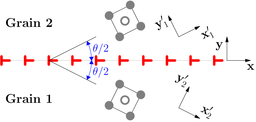
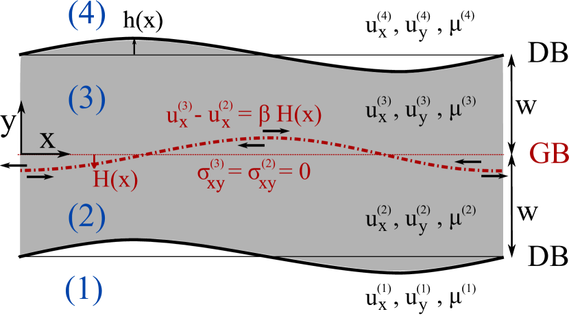
Figure 3: Schematic representation of lamellar precipitate geometry. (a) A low-angle symmetrical tilt GB of angle $\theta$ with the reference frame $(x,y)$ and the frames $(x_{1}^{\prime},y_{1}^{\prime})$ and $(x_{2}^{\prime},y_{2}^{\prime})$ associated with both grains. (b) a GB centered on a slightly perturbed lamellar precipitate. We distinguish four regions (numbered 1 to 4). The displacement fields and chemical potentials in the different regions are respectively denoted $u_{x}^{(n)}$, $u_{y}^{(n)}$ and $\mu^{(n)}$ ($n=1...4$). The horizontal arrows show the directions of grain translation resulting from GB coupled motion via Eq. (1), which relaxes the shear stress induced by the perturbation of the surface of the precipitate.

III.1 Elastostatic equations

We consider a straight symmetric tilt grain boundary of angle $\theta$ obtained from a rotation of the two grains of angles $\pm\theta/2$ around the $z$-axis as depicted in Fig. 3.a. For low angle GBs, this tilt grain boundary can be seen as a wall of edge dislocations.

We consider that the reference frame $(x,y)$ coincides with the cubic axes of the crystal structure. In this frame, the elastic constants are $\mathrm{bar}{C}_{11}=\mathrm{bar}{C}_{22}=\mathrm{bar}{C}_{33}$, $\mathrm{bar}{C}_{12}=\mathrm{bar}{C}_{13}=\mathrm{bar}{C}_{23}$ and $\mathrm{bar}{C}_{44}=\mathrm{bar}{C}_{55}=\mathrm{bar}{C}_{66}$. The system is invariant along the $z$ direction such that we can consider plain strain conditions. We define $S$ as the anisotropy coefficient by:

$$S=1-\frac{\mathrm{bar}{C}_{11}-\mathrm{bar}{C}_{12}}{2\mathrm{bar}{C}_{44}}.$$ (18)

We note that for isotropic elasticity, we have $S=0$. In the frames $(x^{\prime}_{1},y^{\prime}_{1})$ and $(x^{\prime}_{2},y^{\prime}_{2})$ associated to the grains rotated by an angle $\pm\theta/2$, the values of the elastic constants are given by:

$$C_{11}(\psi)= \mathrm{bar}{C}_{11}+S\mathrm{bar}{C}_{44}\sin^{2}(2\psi),$$ (19)

$$C_{12}(\psi)= \mathrm{bar}{C}_{12}-S\mathrm{bar}{C}_{44}\sin^{2}(2\psi),$$ (20)

$$C_{44}(\psi)= \mathrm{bar}{C}_{44}-S\mathrm{bar}{C}_{44}\sin^{2}(2\psi),$$ (21)

$$C_{14}(\psi)= \frac{S\mathrm{bar}{C}_{44}}{2}\sin(4\psi)$$ (22)

where $\psi=\pm\theta/2$ is the rotation angle between the crystal axis of the grains 1 and 2 and the reference frame.

To keep the elastostatic equations analytically solvable, we consider the limit of small $\theta$ where the elastic constants are the same in both grains and in the reference frame and we note them $C_{11}$, $C_{12}$ and $C_{44}$.

We consider that the concentration is homogeneous in the different domains and is denoted by $c^{(n)}$ (where the superscript $(n)$ denotes different domains, $n=1\dots 4$). The stresses can therefore be simply expressed in terms of the displacements in the different domains:

$$\sigma^{(n)}_{xx}= C_{11}(\partial_{x}u^{(n)}_{x}-\varepsilon_{0}c^{(n)})+C_{12}(\partial_{y}u^{(n)}_{y}-\varepsilon_{0}c^{(n)})$$ (23)

$$\sigma^{(n)}_{yy}= C_{12}(\partial_{x}u^{(n)}_{x}-\varepsilon_{0}c^{(n)})+C_{11}(\partial_{y}u^{(n)}_{y}-\varepsilon_{0}c^{(n)})$$ (24)

$$\sigma^{(n)}_{xy}= C_{44}(\partial_{x}u^{(n)}_{y}+\partial_{y}u^{(n)}_{x})$$ (25)

where the coordinate $x$ and $y$ refer to the reference basis $(x,y)$. Substituting these equations for stresses into the elastic equilibrium $\nabla\cdot\sigma=0$, we obtain the following elastostatic equations in terms of the displacements fields:

$$C_{11}\frac{\partial^{2}u^{(n)}_{x}}{\partial x^{2}}+C_{44}\frac{\partial^{2}u^{(n)}_{x}}{\partial y^{2}}+(C_{12}+C_{44})\frac{\partial^{2}u^{(n)}_{y}}{\partial x\partial y}= 0$$ (26)

$$(C_{12}+C_{44})\frac{\partial^{2}u^{(n)}_{x}}{\partial x\partial y}+C_{44}\frac{\partial^{2}u^{(n)}_{y}}{\partial x^{2}}+C_{11}\frac{\partial^{2}u^{(n)}_{y}}{\partial y^{2}}= 0$$ (27)

III.2 Non-perturbed problem

We first consider the non-perturbed problem where the DBs and the GB are perfectly straight ($h(x)=H(x)=0$) and solve for the equilibrium displacement field $\mathrm{bar}{u}$ and composition field. In this case, the problem is invariant along the $x$ direction and $\mathrm{bar}{u}_{x}=0$ in all the domains. For the component $\mathrm{bar}{u}_{y}$, Eqs. (26-27) admit the following solution in the different domains

$$\mathrm{bar}{u}_{y}^{(1)}= \alpha^{-}(y+w)-\alpha^{+}w$$

$$\mathrm{bar}{u}_{y}^{(2)}= \mathrm{bar}{u}_{y}^{(3)}=\alpha^{+}y$$ (28)

$$\mathrm{bar}{u}_{y}^{(4)}= \alpha^{-}(y-w)+\alpha^{+}w$$

where $\alpha^{+}=(C_{11}+C_{12})\varepsilon_{0}c^{+}/C_{11}=\varepsilon_{0}c^{+}\left(1+\frac{1}{\zeta}\right)$ and $\alpha^{-}=(C_{11}+C_{12})\varepsilon_{0}c^{-}/C_{11}=\varepsilon_{0}c^{-}\left(1+\frac{1}{\zeta}\right)$ with $\zeta=C_{11}/C_{12}$.

Because of the stresses arising from the precipitate eigenstrain, the equilibrium concentrations $c^{+}$ and $c^{-}$ inside and outside the precipitate differ slightly from $c_{0}^{+}$ and $c_{0}^{-}$. This deviation can be computed by minimizing the total free energy with respect to $\Delta c=c_{0}^{+}-c^{+}=c^{-}-c_{0}^{-}$. The free energy is minimum for

$$\Delta c=\frac{1}{2}\left[(c_{0}^{+}-c_{0}^{-})-\sqrt{(c_{0}^{+}-c_{0}^{-})^{2}-\frac{(C_{11}^{2}-C_{12}^{2})\varepsilon_{0}^{2}}{gC_{11}}}\right].$$ (29)

III.3 Perturbed problem

III.3.1 Solutions of the elastostatic equations

We consider now that the DBs position are perturbed by a periodic function $h(x)=h_{0}\sin(kx)$ whose amplitude $h_{0}$ is assumed to be small compared to its wave length $2\pi/k$ and the width of the precipitate $w$. The total displacement $u^{(n)}(x,y)$ can be decomposed into a non-perturbed part $\mathrm{bar}{u}^{(n)}(x,y)$ derived in Equation 28 and a perturbed part $\tilde{u}^{(n)}(x,y)$ arising from the perturbation:

$$u_{x}^{(n)}(x,y)= \mathrm{bar}{u}_{x}^{(n)}(x,y)+\tilde{u}_{x}^{(n)}(x,y)$$ (30)

$$u_{y}^{(n)}(x,y)= \mathrm{bar}{u}_{y}^{(n)}(x,y)+\tilde{u}_{y}^{(n)}(x,y)$$ (31)

Following the supplemental material of Ref. [Karma et al., 2012], we consider that the perturbed displacements take the following form in the different domains:

• In domain (1):

  $$\tilde{u}_{x}^{(1)}= \operatorname{Re}\left\{e^{ikx}(A_{1}e^{-ikp_{1}(y+w)}+B_{1}e^{-ikp_{2}(y+w)})\right\}$$ (32)

  $$\tilde{u}_{y}^{(1)}= \operatorname{Re}\left\{e^{ikx}(M_{1}A_{1}e^{-ikp_{1}(y+w)}+M_{2}B_{1}e^{-ikp_{2}(y+w)})\right\}$$ (33)

• In domain (2):

  $$\tilde{u}_{x}^{(2)}= \operatorname{Re}\left\{e^{ikx}(A_{2}e^{ikp_{1}(y+w)}+B_{2}e^{ikp_{2}(y+w)})\right\}+\operatorname{Re}\left\{e^{ikx}(C_{2}e^{-ikp_{1}y}+D_{2}e^{-ikp_{2}y})\right\}$$ (34)

  $$\tilde{u}_{y}^{(2)}= -\operatorname{Re}\left\{e^{ikx}(M_{1}A_{2}e^{ikp_{1}(y+w)}+M_{2}B_{2}e^{ikp_{2}(y+w)})\right\}+\operatorname{Re}\left\{[e^{ikx}(M_{1}C_{2}e^{-ikp_{1}y}+M_{2}D_{2}e^{-ikp_{2}y})\right\}$$

• In domain (3):

  $$\tilde{u}_{x}^{(3)}= \operatorname{Re}\left\{e^{ikx}(A_{3}e^{-ikp_{1}(y-w)}+B_{3}e^{-ikp_{2}(y-w)})\right\}+\operatorname{Re}\left\{e^{ikx}(C_{3}e^{ikp_{1}y}+D_{3}e^{ikp_{2}y})\right\}$$ (36)

  $$\tilde{u}_{y}^{(3)}= \operatorname{Re}\left\{e^{ikx}(M_{1}A_{3}e^{-ikp_{1}(y-w)}+M_{2}B_{3}e^{-ikp_{2}(y-w)})\right\}-\operatorname{Re}\left\{e^{ikx}(M_{1}C_{3}e^{ikp_{1}y}+M_{2}D_{3}e^{ikp_{2}y})\right\}$$

• In domain (4):

  $$\tilde{u}_{x}^{(4)}= \operatorname{Re}\left\{e^{ikx}(A_{4}e^{ikp_{1}(y-w)}+B_{4}e^{ikp_{2}(y-w)})\right\}$$ (38)

  $$\tilde{u}_{y}^{(4)}= -\operatorname{Re}\left\{e^{ikx}(M_{1}A_{4}e^{ikp_{1}(y-w)}+M_{2}B_{4}e^{ikp_{2}(y-w)})\right\},$$ (39)

where $A_{i}$, $B_{i}$, $C_{i}$, $D_{i}$, $M_{i}$ and $p_{i}$ are constants left to be determined. One can show (see Karma et al., 2012) that these equations are solutions of the elastostatic equations Equations 26 and 27 only if the coefficients $M_{1}$ and $M_{2}$ are written as:

$$M_{1}= \frac{(C_{12}+C_{44})p_{1}}{C_{44}+C_{11}p_{1}^{2}}$$ (40)

$$M_{2}= \frac{(C_{12}+C_{44})p_{2}}{C_{44}+C_{11}p_{2}^{2}},$$ (41)

where $p_{1}$ and $p_{2}$ are solutions of the equation

$$p^{4}+\frac{C_{11}^{2}-C_{12}^{2}-2C_{12}C_{44}}{C_{11}C_{44}}p^{2}+1=0.$$ (42)

This polynomial admits two complex roots of the form

$$p_{1}=e^{i\xi},\qquad p_{2}=-e^{-i\xi}$$ (43)

with

$$\xi=\frac{1}{2}\arccos\frac{C_{12}^{2}-C_{11}^{2}+2C_{12}C_{44}}{2C_{11}C_{44}}.$$ (44)

In the limiting case of isotropic elasticity, $p_{1}=p_{2}=i$ and Equations 32 to 39 reduce to the displacements function used in Refs. [Srolovitz, 1989],[Karma et al., 2012] and [Geslin et al., 2015].

The other coefficients $A_{i}$, $B_{i}$, $C_{i}$, $D_{i}$ can be determined from the boundary conditions at the DBs and GB as detailed in the following sections.

III.3.2 Boundary conditions on the DBs

We first examine the boundary conditions at the DB located at $y=w+h(x)$ separating domains (3) and (4). Because the DB is coherent, the total displacement $u(x,y)$ must be continuous across the boundary. We first consider the continuity of the $x$-component: $u_{x}^{(3)}(x,w+h(x))=u_{x}^{(4)}(x,w+h(x))$. Using Taylor expansions around $y=w$ and keeping only the lowest order terms in $h_{0}k$ yields a continuity equation on the perturbed part of the displacements:

$$\tilde{u}_{x}^{(4)}(x,w)=\tilde{u}_{x}^{(3)}(x,w).$$ (45)

For the same boundary, a similar procedure applied to the component $u_{y}$ yields

$$\tilde{u}_{y}^{(4)}(x,w)=\tilde{u}_{y}^{(3)}(x,w)+\alpha h(x),$$ (46)

where $\alpha=\alpha^{+}-\alpha^{-}=\varepsilon_{0}\left(1+\frac{1}{\zeta}\right)(c^{+}-c^{-})$.

Also, the stress vector across the DBs of normal $\mathbb{n}$ defined as $\mathbb{T}=[T_{x},T_{y}]=\bm{\sigma}\cdot\mathbb{n}$ must be continuous.

Substituting Equations 30 and 31 into Equations 23, 24 and 25 and using Equation 28, we get the stress expressed in terms of the perturbed displacements in different domains:

$$\sigma_{xx}^{(n)}= C_{11}\partial_{x}\tilde{u}^{(n)}_{x}+C_{12}\partial_{y}\tilde{u}^{(n)}_{y}-\frac{C_{11}^{2}-C_{12}^{2}}{C_{11}}\varepsilon_{0}c^{(n)}$$

$$\sigma_{yy}^{(n)}= C_{11}\partial_{y}\tilde{u}^{(n)}_{y}+C_{12}\partial_{x}\tilde{u}^{(n)}_{x}$$ (47)

$$\sigma_{xy}^{(n)}= C_{44}[\partial_{y}\tilde{u}^{(n)}_{x}+\partial_{x}\tilde{u}^{(n)}_{y}]$$

where $c^{(2)}=c^{(3)}=c^{+}$ and $c^{(1)}=c^{(4)}=c^{-}$.

Substituting Equation 47 for domains (3) and (4) into the continuity of the stress vector and keeping only the lowest order terms after performing Taylor expansions in $h_{0}k\ll 1$, we obtain two additional boundary conditions on the perturbed displacement components $\tilde{u}_{x}$ and $\tilde{u}_{y}$. Finally, the boundary conditions on the DB located at $y=w+h(x)$ can be summarized as follow:

$$\tilde{u}_{x}^{(4)}(x,w)-\tilde{u}_{x}^{(3)}(x,w)= 0$$ (48)

$$\tilde{u}_{y}^{(4)}(x,w)-\tilde{u}_{y}^{(3)}(x,w)= \alpha h(x)$$ (49)

$$\left[\partial_{y}\tilde{u}_{x}^{(4)}+\partial_{x}\tilde{u}_{y}^{(4)}\right]_{y=w}-\left[\partial_{y}\tilde{u}_{x}^{(3)}+\partial_{x}\tilde{u}_{y}^{(3)}\right]_{y=w}= \frac{C_{11}-C_{12}}{C_{44}}\alpha h^{\prime}(x)$$ (50)

$$\left[\partial_{x}\tilde{u}_{x}^{(4)}+\zeta\partial_{y}\tilde{u}_{y}^{(4)}\right]_{y=w}-\left[\partial_{x}\tilde{u}_{x}^{(3)}+\zeta\partial_{y}\tilde{u}_{y}^{(3)}\right]_{y=w}= 0$$ (51)

We derive similar boundary conditions for the DB between domains (1) and (2) located at $y=-w+h(x)$:

$$\tilde{u}_{x}^{(1)}(x,-w)-\tilde{u}_{x}^{(2)}(x,-w)= 0$$ (52)

$$\tilde{u}_{y}^{(1)}(x,-w)-\tilde{u}_{y}^{(2)}(x,-w)= \alpha h(x)$$ (53)

$$\left[\partial_{y}\tilde{u}_{x}^{(1)}+\partial_{x}\tilde{u}_{y}^{(1)}\right]_{y=-w}-\left[\partial_{y}\tilde{u}_{x}^{(2)}+\partial_{x}\tilde{u}_{y}^{(2)}\right]_{y=-w}= \frac{C_{11}-C_{12}}{C_{44}}\alpha h^{\prime}(x)$$ (54)

$$\left[\partial_{x}\tilde{u}_{x}^{(1)}+\zeta\partial_{y}\tilde{u}_{y}^{(1)}\right]_{y=-w}-\left[\partial_{x}\tilde{u}_{x}^{(2)}+\zeta\partial_{y}\tilde{u}_{y}^{(2)}\right]_{y=-w}= 0$$ (55)

III.3.3 Boundary conditions on the GB

The perturbation of DBs produces shear stresses on the GB which is considered to relax entirely the shear stresses by coupling. We note $H(x)$ the perturbation of the GB position whose amplitude is assumed to be of the order of $h_{0}$. Boundary conditions accounting for the GB coupling behavior can then be written assuming that the GB behaves like a sharp interface located at $H(x)$.

As explained in Section I, the coupling behavior of the GB can be translated into the well-known geometrical relation of Equation 1 between the normal GB velocity $v_{n}$ and the velocity of parallel grain translation $v_{\parallel}$ Cahn and Taylor (2004); Cahn et al. (2006). A simple time integration of this equation leads to a relationship between the GB perturbation, $H(x)$, and the jump of the total displacement $u_{x}$ across the GB. After performing Taylor expansions around $y=H(x)$ and keeping the dominant term, we obtain

$$\tilde{u}_{x}^{(3)}(x,0)-\tilde{u}_{x}^{(2)}(x,0)=\beta H(x).$$ (56)

Substituting the displacements $\tilde{u}_{x}^{(2)}$ and $\tilde{u}_{x}^{(3)}$ described in Equations 34 and 36 into this equation, we deduce that the function $H(x)$ takes the form $H(x)=H_{0}\cos(kx)$, where $H_{0}$ is a constant unknown at the moment. Therefore, the GB perturbation $H(x)$ is out of phase compared to the DB perturbation $h(x)$, as depicted in Figure 1.

The coupling behavior of the GB does not influence the component $u_{y}$ of the displacement field, which remains continuous across the boundary. The procedure explained in section III.3.2 can be applied straightforwardly to the component $u_{y}$, yielding:

$$\tilde{u}_{y}^{(3)}(x,0)-\tilde{u}_{y}^{(2)}(x,0)=0.$$ (57)

Just like in the case of DBs, the components of the stress vector $\mathbb{T}$ is continuous across the GB. The continuity of the component $T_{x}$ leads to the following equation:

$$\left[\partial_{x}\tilde{u}_{x}^{(3)}+\zeta\partial_{y}\tilde{u}_{y}^{(3)}\right]_{y=0}-\left[\partial_{x}\tilde{u}_{x}^{(2)}+\zeta\partial_{y}\tilde{u}_{y}^{(2)}\right]_{y=0}=0$$ (58)

In addition to the continuity of the component $T_{y}$, we assume that the GB relaxes completely the shear stresses through coupling. In other words, the GB adapts its shape to the shear stress environment produced by the perturbation on the DBs such that the shear stresses vanish at $y=H(x)$. This leads to the following relation on the perturbed displacements:

$$\left[\partial_{y}\tilde{u}_{x}^{(2)}+\partial_{x}\tilde{u}_{y}^{(2)}\right]_{y=0}= 0$$ (59)

$$\left[\partial_{y}\tilde{u}_{x}^{(3)}+\partial_{x}\tilde{u}_{y}^{(3)}\right]_{y=0}= 0$$ (60)

Finally, we obtained five boundary conditions (Equations 57 to 60) that have to be fulfilled on the GB by the displacement field.

III.3.4 Solution of the elastostatic equations

Substituting the expression of the displacements Equations 32 to 39 into the boundary conditions (48)-(60) yields 13 linear equations. The 13 unknowns of the problem ($A_{i}$, $B_{i}$, $C_{i}$, $D_{i}$, $H_{0}$) are then determined uniquely by solving the linear system of equations. In particular, we obtain an expression of the GB amplitude $H_{0}$:

$$H_{0}= \left(2ih_{0}(M_{1}p_{1}-M_{2}p_{2})\alpha(1+\zeta)\left[(e^{ikp_{1}w}M_{2}(-M_{1}+p_{1})-e^{ikp_{2}w}M_{1}(-M_{2}+p_{2}))(-1+\zeta)C_{12}\right.\right.$$

$$+\left.\left.(e^{ikp_{1}w}-e^{ikp_{2}w})(-M_{1}+p_{1})(-M_{2}+p_{2})C_{44}\right]\right)$$ (61)

$$/\left((M_{2}p_{1}-M_{1}p_{2})\left[-p_{1}+p_{2}+M_{1}(1+M_{2}(p_{1}-p_{2})\zeta-p_{1}p_{2}\zeta)+M_{2}(-1+p_{1}p_{2}\zeta)\right]C_{44}\beta\right)$$

The full expression of the other unknowns $A_{i}$, $B_{i}$ $C_{i}$ and $D_{i}$ are quite lengthy and are detailed in appendix B. To highlight the influence of the anisotropic elasticity on the instability, we express the elastic constants $C_{11}$, $C_{12}$ and $C_{44}$ as a function of an equivalent shear modulus $G=C_{44}$, Poisson’s ratio $\nu=C_{12}/(C_{11}+C_{12})$ and the anisotropic factor $S=1-\frac{C_{11}-C_{12}}{2C_{44}}$:

$$C_{44}= G$$ (62)

$$C_{12}= \frac{2(1-S)G\nu}{1-2\nu}$$ (63)

$$C_{11}= \frac{2(1-S)G(1-\nu)}{1-2\nu}$$ (64)

Finally, we expand Equation 44 in the limit of small $S$: $\xi=\left(\pi-\sqrt{2S/(1-\nu)}\right)/2$. After substituting these expressions into Equation 61 and performing a Taylor expansion for small $S$, we obtain

$$H_{0}=-\frac{4\varepsilon_{0}(c^{+}-c^{-})h_{0}e^{-kw}}{\beta}+\frac{\varepsilon_{0}(c^{+}-c^{-})h_{0}e^{-kw}(1-3kw+k^{2}w^{2})S}{\beta(1-\nu)}+O(S^{3/2})$$ (65)

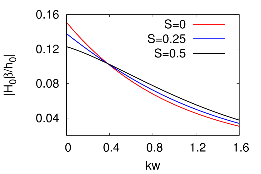
Figure 4: Ratio $|H_{0}\beta/h_{0}|$ versus the dimensionless wave-vector $kw$ obtained from Equation 65 for different values of the anisotropic coefficient $S$, showing the influence of the elastic anisotropy on the relative amplitudes of the GB and DB perturbations.

In the isotropic limit ($S=0$), we recover exactly our previously derived result (Eq. (13) in Ref. [Geslin et al., 2015]). The role of anisotropic elasticity enters as a correction proportional to $\varepsilon_{0}h_{0}/\beta$ in the limit of small $S$. We note that the term $(1-3kw+k^{2}w^{2})$ entering this corrective term can be positive or negative depending on value the $kw$. This is illustrated in Figure 4 where $|H_{0}\beta/h_{0}|$ is plotted as a function of $kw$ for different values of $S$.

III.4 Linear stability analysis

In the previous section, we solved the elastostatic equations when the DB position is modified by a periodic perturbation. In this section, we formulate a Stefan-like free boundary problem that governs the diffusion-controlled motion of the DBs in the sharp-interface limit where the DB width is much smaller than the perturbation wavelength. Furthermore, we perform a linear stability analysis of the evolution equations for the DBs to obtain the growth rate of the morphological instability driven by the elastic interaction between the DBs and GB. This analysis makes use of the results of the previous section for the stresses on the perturbed DBs.

Far from the DBs, the concentration is close to its equilibrium value $\mathrm{bar}{c}^{\pm}$ such that Equation 12 reduces to the diffusion equation. Moreover, in this limit, the chemical potential defined as $\mu=\delta F/\delta c$ is proportional to the solute concentration. Therefore, the same diffusion equation holds for $\mu$:

$$\frac{\partial\mu^{(n)}}{\partial t}=D\nabla^{2}\mu^{(n)},\quad n=1\dots 4,$$ (66)

where $D=Mf_{dw}^{\prime\prime}(c^{\pm})$ is the diffusion coefficient.

Similarly to what has been done for the displacement field in the previous section, the chemical potential is decomposed as a sum $\mu=\mathrm{bar}{\mu}+\tilde{\mu}$ where $\mathrm{bar}{\mu}$ is the equilibrium chemical potential for the non-perturbed configuration and $\tilde{\mu}$ is a small variation due to DB perturbations.

We first consider the non-perturbed DB located between domains (1) and (2), at $y=-w$. The composition field $c(x,y)$ does not depend on $x$ and adopts an equilibrium profile along $y$ denoted by $\mathrm{bar}{c}(y)$, reaching the values $\mathrm{bar}{c}^{-}$ and $\mathrm{bar}{c}^{+}$ in domains (1) and (2) respectively. At equilibrium, the chemical potential is constant across the DB interface and is given by

$$\mathrm{bar}{\mu}=f_{dw}^{\prime}(\mathrm{bar}{c}(y))-\varepsilon_{0}(\mathrm{bar}{\sigma}_{xx}(y)+\mathrm{bar}{\sigma}_{yy}(y))-K\partial_{y}^{2}\mathrm{bar}{c}(y)$$ (67)

where $\mathrm{bar}{\sigma}_{xx}(y)$ and $\mathrm{bar}{\sigma}_{yy}(y)$ are the stress profiles along the $y$ direction. The second term emerges from the derivative of the elastic energy density Equation 5 lineralized for small deformations $f_{el}^{lin}=\frac{1}{2}\sigma_{ij}(\varepsilon_{ij}-\delta_{ij}\varepsilon_{0}c)$.

We then consider a perturbation $h(x)$ of the DBs and elastic displacements. Using the linearity of elasticity, the total stress fields can be written as $\sigma_{ij}=\mathrm{bar}{\sigma}_{ij}+\tilde{\sigma}_{ij}$, where $\sigma_{ij}$ is the stress field induced by the perturbation. Considering that the perturbation $h(x)$ is a slowly varying function of $x$, we can assume that, in the vicinity of the DB, the concentration field takes the form $c(x,y)\approx\mathrm{bar}{c}(y-h(x))$. Substituting these expressions for the stress and composition fields into the definition of the chemical potential and keeping only the dominant terms, we obtain

$$\mu=\mathrm{bar}{\mu}-\varepsilon_{0}(\tilde{\sigma}_{xx}+\tilde{\sigma}_{yy})+K\partial_{y}\mathrm{bar}{c}\kappa$$ (68)

where $\kappa$ is the domain interface curvature. The chemical potential $\mu$ and the stress fields $\tilde{\sigma}_{xx}$ and $\tilde{\sigma}_{yy}$ vary on a much larger length-scale than the interface width and can be assumed to be constant across the DB. We then multiply Equation 68 by $\partial_{y}\mathrm{bar}{c}$ and integrate over the interval $[-w-\delta,-w+\delta]$ where $\delta$ is an arbitrary intermediate length, larger than the interface width but much smaller than the characteristic scale on which the stresses and chemical potential vary. We finally obtain the chemical potential acting on the DBs:

$$\mu_{\text{\tiny DB}}=\mathrm{bar}{\mu}-\varepsilon_{0}[\tilde{\sigma}_{xx}+\tilde{\sigma}_{yy}]_{\text{\tiny DB}}+\frac{\gamma\kappa}{\mathrm{bar}{c}^{+}-\mathrm{bar}{c}^{-}}$$ (69)

where $\gamma=K\int_{-w-\delta}^{-w+\delta}(\partial_{y}\mathrm{bar}{c})^{2}dy$ is the interfacial energy and $[\tilde{\sigma}_{xx}+\tilde{\sigma}_{yy}]_{\text{\tiny DB}}$ is the sum of the stresses at the DB.

In the case of a periodic perturbation $h(x)=h_{0}\sin(kx)$, the stresses at the DB are obtained by substituting Equations 32 to 39 into Equation 47 and using the expression of $A_{i}$, $B_{i}$, $C_{i}$ and $D_{i}$ listed in Appendix B. Similarly to the expression of the GB perturbation, the stresses can be expressed as a Taylor expansion, treating the anisotropic coefficient $S$ as a small parameter:

$$[\tilde{\sigma}_{xx}+\tilde{\sigma}_{yy}]_{DB}= \operatorname{Re}\{-k(C_{11}+C_{12})[(A_{1}+B_{1})-(M_{1}p_{1}A_{1}+M_{2}p_{2}B_{1})]_{y=-w}\}$$ (70)

$$= \operatorname{Re}\{-k(C_{11}+C_{12})[(A_{4}+B_{4})-(M_{1}p_{1}A_{4}+M_{2}p_{2}B_{4})]_{y=w}\}$$

$$= \left\{-\frac{4\varepsilon_{0}(\mathrm{bar}{c}^{+}-\mathrm{bar}{c}^{-})kGe^{-2kw}}{1-\nu}+\frac{\varepsilon_{0}(\mathrm{bar}{c}^{+}-\mathrm{bar}{c}^{-})kGS[1+(4(1-\nu)-4kw+2k^{2}w^{2})e^{-2kw}]}{(1-\nu)^{2}}+O(S^{3/2})\right\}h$$

In the limit of isotropic elasticity ($S=0$), we recover the stresses obtained in Ref. [Geslin et al., 2015].

We now perform a linear stability analysis by considering that the amplitude of the perturbation $h_{0}(t)$ evolves exponentially in time: $h_{0}(t)=h_{i}\exp(\omega_{k}t)$, with $\omega_{k}$ the growth rate of the instability and $h_{i}$ the initial amplitude of the perturbation.

For simplicity, we define the function

$$\Gamma(k)=-\frac{\varepsilon_{0}[\tilde{\sigma}_{xx}+\tilde{\sigma}_{yy}]_{\text{\tiny DB}}}{h(x,t)}+\frac{\gamma k^{2}}{\mathrm{bar}{c}^{+}-\mathrm{bar}{c}^{-}},$$ (72)

such that the chemical potential on the DB between domains (1) and (2) is simply given by

$$\mu_{\text{\tiny DB}}^{(1,2)}(t)=\mathrm{bar}{\mu}+\Gamma(k)h(x,t)$$ (73)

Similarly, the chemical potential on the DB between domains (3) and (4) is:

$$\mu_{\text{\tiny DB}}^{(3,4)}(t)=\mathrm{bar}{\mu}-\Gamma(k)h(x,t).$$ (74)

Equations 73 and 74 serve as boundary conditions for the solution of Equation 66. In addition, two additional boundary conditions are obtained by considering that the chemical potential reaches $\mathrm{bar}{\mu}$ far from the DBs (i.e. for $y\to\pm\infty$). The solution of Equation 66 satisfying these boundary conditions is of the form

$$\mu^{(1)}= \mathrm{bar}{\mu}+\Gamma(k)e^{q(y+w)}h(x,t)$$ (75)

$$\mu^{(n)}= \mathrm{bar}{\mu}-\Gamma(k)\frac{\sinh(qy)}{\sinh(qw)}h(x,t),\quad n=2,3$$ (76)

$$\mu^{(4)}= \mathrm{bar}{\mu}-\Gamma(k)e^{-q(y-w)}h(x,t)$$ (77)

where $q=\sqrt{k^{2}+\omega_{k}/D}$.

Next, the normal velocity of the DBs is given by the mass conservation (Stefan-like) condition

$$v_{\text{\tiny DB}}=-\frac{M}{\mathrm{bar}{c}^{+}-\mathrm{bar}{c}^{-}}\llbracket\partial_{y}\mu\rrbracket_{\text{\tiny DB}},$$ (78)

where the double brackets denotes the jump of the normal gradient of chemical potential $\partial_{y}\mu$ across the DB, neglecting higher order nonlinear terms originating from the change of normal direction induced by the perturbation of the DB (i.e. $\sqrt{1+(\partial_{x}h)^{2}}\approx 1$). Using the fact that $v_{\text{\tiny DB}}=\partial_{t}h=\omega_{k}h(x,t)$ and Equations 75 to 77 to evaluate the right-hand-side of Equation 78, we obtain an implicit transcendental equation for $\omega_{k}$:

$$\omega_{k}=\frac{M\Gamma(k)}{c^{+}-c^{-}}\sqrt{\frac{\omega_{k}}{D}+k^{2}}\left(1+\coth\left(w\sqrt{\frac{\omega_{k}}{D}+k^{2}}\right)\right).$$ (79)

We can consider the quasistatic limit where the concentration field that evolves on a time-scale $1/Dk^{2}$ reaches quickly an equilibrium profile compared to the time-scale of the evolution of the DB $1/\omega_{k}$. Our simulations are performed within this quasistatic limit. With $\omega_{k}\ll Dk^{2}$, $q\simeq k$ and Equation 79 reduces to a straightforward expression for $\omega_{k}$:

$$\omega_{k}=\frac{M\Gamma(k)k}{c^{+}-c^{-}}\left(1+\coth(kw)\right)$$ (80)

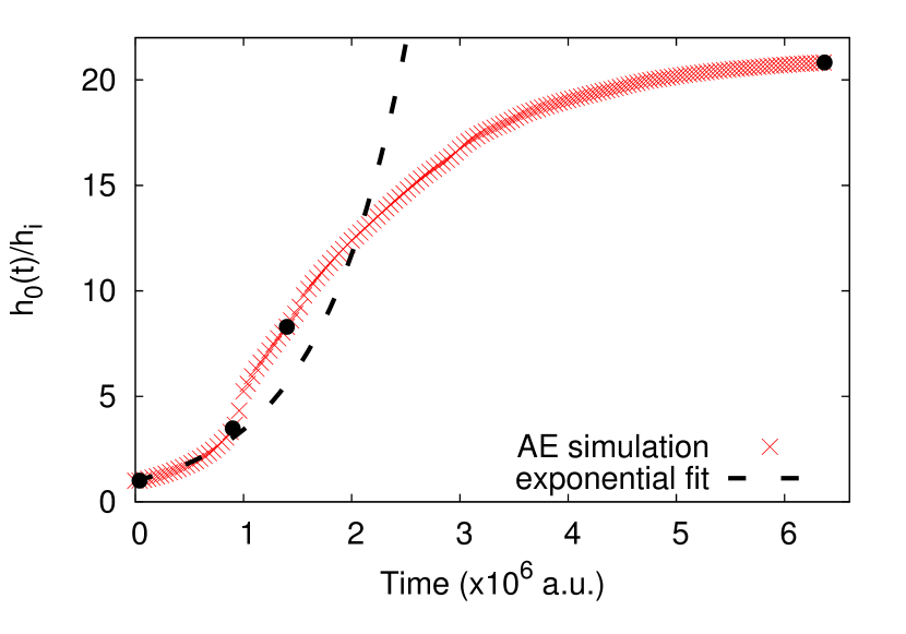
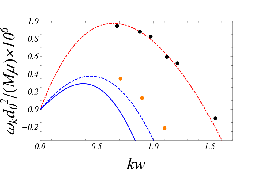
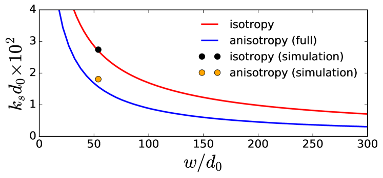
Figure 5: (a) Amplitude of perturbed DB v.s. time for the simulation shown in Figure 1. Black dots locate the snapshots in Figure 1. The dashed line represents the exponential fit performed to obtain the growth rate of the instability. (b) Dimensionless growth rate $\omega_{k}$ as a function of the normalized wavevector $kw$ ($w$ is the half-width of the compositional domain) in the isotropic case (red) and anisotropic case (blue) with $S=0.5$. In both cases, $w=32a$ and $\varepsilon_{0}=0.043$ while the GB misorientation is $7.2\mathrm{\SIUnitSymbolDegree}$ and $11.5\mathrm{\SIUnitSymbolDegree}$ in the isotropic and anisotropic case, respectively. For the anisotropic case, both the exact solution (derived using Equation 70) and the approximate solution (derived using Section III.4) are represented respectively with a dashed and continuous line. (c) Marginal wavevector $k_{s}$ as a function of the domain half-width $w$ for both isotropic (red) and anisotropic (blue) elasticity. The theoretical prediction in the anisotropic case is obtained from the exact solution (derived using Equation 70).

We note that for typical material values of $\nu<1/2$, the second term of Section III.4 has the same sign as the anisotropic coefficient $S$. Therefore, if $S>0$ ($S<0$), the elastic anisotropy inhibits (promotes) the development of the instability compared to the isotropic case.

To check the validity of this analysis, we performed AE simulations with both the isotropic hexagonal and anisotropic BCC models. In both cases, we choose $C_{44}=$39\text{\,}\mathrm{G}\mathrm{P}\mathrm{a}$$. In the BCC AE model, we have necessarily $C_{11}=2C_{12}=2C_{44}$, fixing $S=0.5$. The misfit eigenstrain is $\varepsilon_{0}=0.043$. In addition, the GB misorientation is $7.2\mathrm{\SIUnitSymbolDegree}$ and $11.5\mathrm{\SIUnitSymbolDegree}$ in the isotropic and anisotropic simulations, respectively.

To obtain the growth rate numerically, we perform simulations where the DBs are initially gently deformed from their planar configuration with a small amplitude sinusoidal perturbation. As demonstrated by the linear stability analysis, the stresses induced by this perturbation lead to an increase of the perturbation amplitude $h_{0}(t)$. Figure 5.a displays the amplitude of the DB perturbation as a function of time for the simulation presented in Figure 1. The black dots along the curve locate the snapshots shown in Figure 1. We can distinguish two regimes. First, the perturbation amplitude grows exponentially with time as predicted by the linear stability analysis. The growth rate of the simulation is obtained by performing an exponential fit on this part of the curve. Second, at longer times, nonlinearities play a significant role and are responsible for the deviation of the simulation results from the exponential fit. As depicted in Figure 1.c, the DBs collide with the GB, leading to a highly non-linear regime where GB breaks-up and the position of the individual dislocations are relaxed by both glide and climb (see Figure 1.d).

The growth rates are obtained for different simulations performed with various wavevector $k$ and for a precipitate width $w=32\,a$. We note that large wave-lengths (i.e. $kw<0.7$) are not investigated computationally due to the large simulation box sizes necessary to explore this part of the dispersion diagram. For both the isotropic and anisotropic AE models, the results are compared to analytical predictions in Figure 5.b. For the sake of consistency with Ref. [Geslin et al., 2015], the growth rate $\omega_{k}$ is normalized by the characteristic time $d_{0}^{2}/GM$ where $d_{0}$ is defined for an isotropic material by $d_{0}=\gamma(1-\nu)/[8G\varepsilon_{0}^{2}(c^{+}-c^{-})]$. As already discussed in Ref. [Geslin et al., 2015], the simulation results in the isotropic case ($S=0$) agree well with the analytical prediction.

As discussed previously, Figure 5.b clearly shows that for our choice of parameters ($S=0.5$), the anisotropic elasticity reduces significantly the growth rate and shifts the unstable range (where $\omega_{k}>0$) to larger wavelengths, therefore inhibiting the instability. This can be understood with the following qualitative argument: in the isotropic case, the Bitter-Crum theorem Bitter (1931); Fratzl et al. (1999) insures that the elastic energy of a precipitate does not depend on its shape. Therefore, the perturbation of the DB interface leads automatically to a decrease of the elastic energy due to the relaxation of the shear stresses at the GBs. If this energy drop compensates the increase of energy attributed to the lengthening of the perturbed DBs, the system is unstable. This reasoning does not hold in the anisotropic case where the Bitter-Crum theorem does not apply. In our case, the lamellar precipitate is oriented along an elastically soft direction. Any perturbation of such a well-oriented precipitate increases the elastic energy. Therefore, the destabilization of the system occurs only if the stress relaxation at the GB compensates this additional amount of energy. We note that a lamellar precipitate oriented along an elastically hard direction (e.g. with a $45\mathrm{\SIUnitSymbolDegree}$ angle with the $x$-axis) is intrinsically unstable Khachaturyan (2013).

The simulations performed with the BCC AE model show a good agreement with the growth rate predicted by the linear stability analysis. The small discrepancy between the numerical and analytical results is attributed to the homogeneous elasticity approximation. Indeed, to perform the linear stability analysis, we considered that the elastic constants are the same in both grains, regardless of the rotations introduced by the GB. Also, numerical limitations such as limited system sizes might also contribute to this small discrepancy.

The marginally stable wavevetor $k_{s}$ defined as the positive root of $\omega_{k}=0$ can be deduced for both numerical and theoretical results and is plotted as a function of the normalized composition domain half-width $w$ in the isotropic and anisotropic case in Figure 5.c. This plot shows again that the elastic anisotropy shifts the domain of instability to longer wavelengths, thus inhibiting the morphological instability. Even though we only presented numerical results for one value of $w$, the dependence of the results on $w$ can be deduced from the predictions of the linear stability analysis. For isotropic elasticity, this analysis predicts that, in the physically relevant limit $w\gg d_{0}$ where the precipitate width is much larger than the microscopic capillary length scale $d_{0}$, the marginally stable wavector $k_{s}\approx\frac{1}{2w}\ln(w/d_{0})$ and the fastest growing wavector $k_{0}\approx C/w$ where $C=0.797...$ is a numerical constant Geslin et al. (2015). The same scalings holds for the anisotropic case but with the constant $C$ depending generally on the magnitude $S$ of the anisotropy. As can be seen in Fig. 5.b, the fastest growing wavector is smaller in the anisotropic case than the isotropic case, consistent with the fact that anisotropy has a stabilizing effect when the lamellar precipitate is oriented along an elastically soft direction. However, in both the isotropic and anisotropic cases, the most unstable wavelength $2\pi/k_{0}$ is proportional to $w$ so that the instability will generally develop on the scale of the precipitate width.

IV Grain boundary break-up

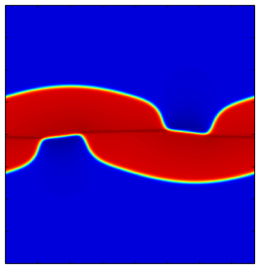
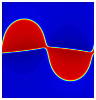
Figure 6: Snapshots of the concentration field during a simulation performed with a GB misorientation angle $\theta=30.4\mathrm{\SIUnitSymbolDegree}$ centered on a lamellar precipitate of eigenstrain $\varepsilon_{0}=0.043$. The system size is $7.8w\times 10.8w$ where $2w$ is the initial width of the precipitate (the vertical length of each frame is smaller than the box dimension). The snapshots correspond to dimensionless times (a) $1.2\times 10^{6}$ and (b) $5.12\times 10^{6}$. See online supplementental materialSup for the movie of this simulation (file movie1.avi).

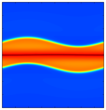
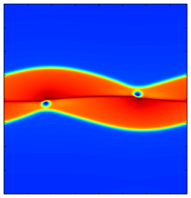
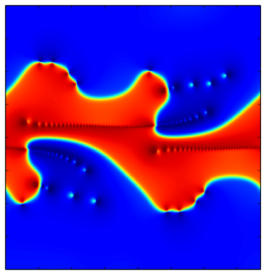
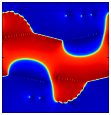
Figure 7: Snapshots of the concentration field during a simulation performed with a GB misorientation angle $\theta=30.4\mathrm{\SIUnitSymbolDegree}$ centered on a lamellar precipitate of eigenstrain $\varepsilon_{0}=0.086$. The system size is $7.8w\times 10.8w$ where $2w$ is the initial width of the precipitate (the vertical length of each frame is smaller than the box dimension). The snapshots correspond to dimensionless times (a) $4\times 10^{3}$, (b) $7.6\times 10^{4}$, (c) $2.84\times 10^{5}$ and (d) $4.2\times 10^{6}$. See online supplementental materialSup for the movie of this simulation (file movie2.avi).

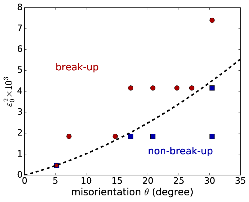
Figure 8: GB behavior as a function of misorientation angle $\theta$ and misfit strain $\varepsilon_{0}$. Simulations where the GB breaks up are represented with red dots while the ones where the GB is morphologically unstable but remains continuous are shown with blue squares. The dashed line is a second order polynomial fit of the boundary between break-up and non-break-up regions of the ($\theta$, $\varepsilon_{0}^{2}$) plane.

In polycrystalline materials, the density and properties of GBs influence significantly the properties of the bulk material. They are preferred nucleation sites for second phase precipitates Sutton and Balluffi (1995). and also facilitate impurities diffusion though a pipe diffusion effect Hirth and Lothe (1968). Moreover, GBs are natural obstacles to dislocation motion, and fine grain structures often present high yield stresses Sutton and Balluffi (1995). Therefore, controlling the GB density and properties is of first importance to obtain high material properties.

The instability described in this article affects significantly the GB and can even lead to the break-up of the GB as shown in Figure 1. For this low angle GB ($\theta=7.2\mathrm{\SIUnitSymbolDegree}$), $\beta=0.126$ and the perturbation of the GB expressed in Equation 65 is significant as shown in Figure 1.b. In the equilibrium state represented in Figure 1.e., the dislocations that were forming the low-angle GB decorate the precipitate interface, relaxing the misfit stresses.

Increasing the GB angle does not modify the development nor the growth rate of the instability. However, for higher misorientation angles, the coupling factor $\beta$ is greater and therefore the amplitude of the GB perturbation is smaller. So, one can expect the influence of the instability on the GB to be less important. Figure 6 shows the late stages of the development of the instability for a misorientation angle $\theta=30.4\mathrm{\SIUnitSymbolDegree}$ GB, everything else being identical to the simulation presented in Figure 1. As expected, the GB is less affected by the instability: its position is only slightly modified and the precipitate shape evolves until the DBs wet the GB. Figure 6.b represents the equilibrium state of the system where the GB remains continuous and the precipitate forms lobes on both sides of the GB. We note here that this destabilization can represent the first stage of development of the Widmanstätten structure found in steel and Ti-based alloys Teixeira et al. (2006); Cheng et al. (2010). It has been shown experimentally that Widmanstätten structures develop in two steps: first, an thin elongated precipitate nucleates on the GB and grow laterally; then, the precipitate develops acicular arms growing perpendicularly to the GB, towards the center of the grain. The instability presented in this paper and more precisely the morphology shown in Figure 6.b could trigger the growth of elongated precipitates perpendicular to the GB.

However, increasing the misfit strain can destabilize a high angle GB as well: Figure 7 shows a simulation performed with $\theta=30.4\mathrm{\SIUnitSymbolDegree}$ and a misfit eigenstrain of $\varepsilon_{0}=0.086$. During the development of the instability, we notice the nucleation of low composition domains close to the GB (blue droplets in Figure 7.b) promoted by the high compressive stress appearing in the vicinity of the deformed GB. Later in the simulation, the high angle GB breaks up (Figure 7.c) and the system relaxes into a configuration presenting two lower angle GBs (Figure 7.d). The equilibrium configuration also shows that dislocations decorate the precipitate surface, relaxing the high misfit stresses.

The appearance of GB break-up then depends on a balance between the misfit stresses and the GB misorientation. This is summarized in Figure 8 where the results of several simulations for various values of the misorientation angle $\theta$ and eigenstrain $\varepsilon_{0}$ are presented: the GB break-up occurs for low angle GBs and high values of $\varepsilon_{0}^{2}$. The dashed line separating both regions serves as a guide to the eye and is linear for small values of the misorientation angle. It also shows that for a large enough misfit, the instability break up all GBs.

V Interaction between circular precipitates and grain boundaries

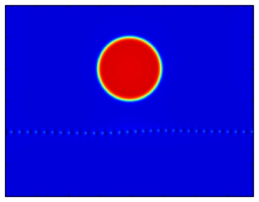
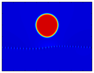
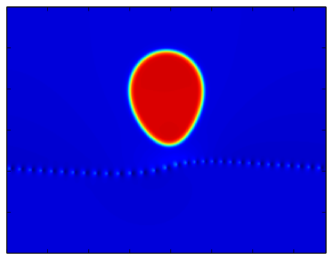
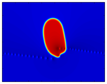
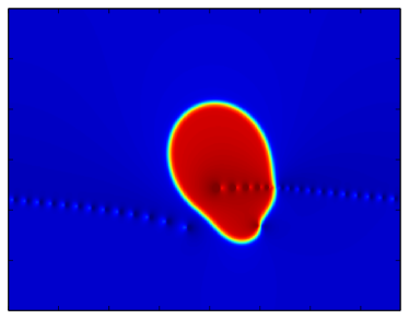
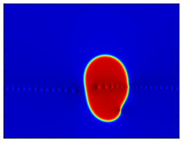
Figure 9: Snapshots of the concentration field during a simulation performed with a GB misorientation $\theta=7.2\mathrm{\SIUnitSymbolDegree}$ and a circular precipitate with a misfit eigenstrain $\varepsilon_{0}=0.043$. The system size is $7.8R\times 11.3R$ where $R$ is the radius of the circular precipitate. The snapshots correspond to dimensionless times (a) $1\times 10^{4}$, (b) $1.6\times 10^{5}$, (c) $5.1\times 10^{5}$, (d) $1.01\times 10^{6}$, (e) $2.72\times 10^{6}$ and (f) $6.18\times 10^{6}$. See online supplementental materialSup for the movie of this simulation (file movie3.avi).

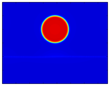
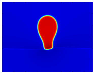
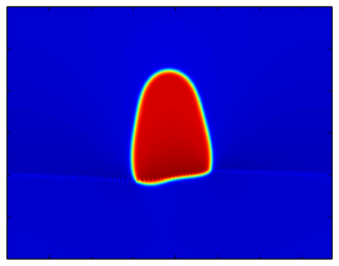
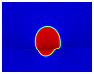
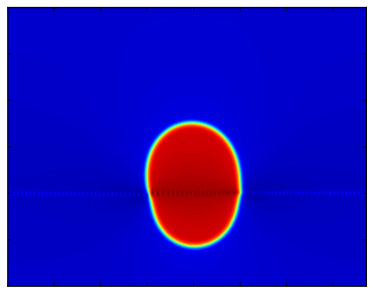
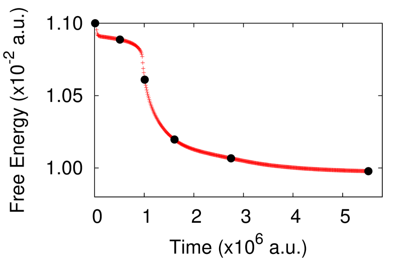
Figure 10: Snapshots of the concentration field during a simulation performed with a GB misorientation $\theta=20.8\mathrm{\SIUnitSymbolDegree}$ and a circular precipitate with a misfit eigenstrain $\varepsilon_{0}=0.043$. The system size is $7.7R\times 10.8R$ where $R$ is the radius of the circular precipitate. The snapshots correspond to dimensionless times (a) $1\times 10^{4}$, (b) $5.1\times 10^{5}$, (c) $1.01\times 10^{6}$, (d) $1.61\times 10^{6}$, (e) $2.75\times 10^{6}$ and (f) $5.52\times 10^{6}$. The evolution of the total free energy is represented in panel (g) in which black dots locate the snapshots in (a-f). See online supplementental materialSup for the movie of this simulation (file movie4.avi).

In the previous sections, we considered configurations consisting of a lamellar precipitate centered on a GB. Even though this geometry is relevant for heterogeneous nucleation of precipitates on GBs, circular precipitates also commonly appear in the vicinity of a GB as exemplified by Ni-Al superalloys Koul and Gessinger (1983); Safari and Nategh (2006); Mitchell et al. (2009). The $\gamma^{\prime}$ precipitates in these alloys are known to influence the GB morphology by causing their serration and this mechanism has been shown to improve the creep properties of the alloy by preventing GB sliding Koul and Gessinger (1983). The GB serration has been proposed to be due to a balance between the elastic energy released by the coherency loss of the precipitate interface in contact with the GB and the GB surface tension Koul and Gessinger (1983); Safari and Nategh (2006), two ingredients that are naturally taken into account in the AE model.

We consider a configuration consisting of a circular precipitate of radius $R=32a$ and of misfit $\varepsilon_{0}=0.043$ located at a distance $2R$ of a symmetrical GB. Snapshots of simulations performed with two different misorientation angles $\theta=7.2\mathrm{\SIUnitSymbolDegree}$ and $\theta=20.8\mathrm{\SIUnitSymbolDegree}$ are presented in Figures 9 and 10, respectively. Even though the circular and lamellar precipitate geometries differ significantly, the simulations reveal that the mechanism of the GB instability is similar in both cases. The GB deforms slightly by shear-coupled motion to relax shear stresses produced by the misfitting particle. In turn, the deformed GB produces an heterogeneous stress field, inducing the migration of the precipitate towards the GB (see Figure 9.a-c and Figure 10.a-b). This migration is mediated by the elongation of the precipitate. The additional surface energy caused by this elongation is compensated by the relaxation of shear stresses by the GB coupling mechanism. Therefore, the interplay between the elastic energy and the surface energy lead to the destabilization of the configuration through a mechanism similar to the morphological instability of lamellar precipitates described previously. Eventually, the misfitting particle enters in contact with the GB. For the low angle GB, the misfit stress is large enough to break-up the GB (see Figure 9.d), allowing the GB dislocations to relax part of the misfit stress. For the higher angle GB, the precipitate interface wets the GB without leading to its break-up (see Figure 10.d). In both cases, the equilibrium configuration show a slightly elliptic precipitate centered on the somewhat perturbed GB. This configuration relaxes the total energy as shown in Figure 10.g.

Despite a large value of the misfit compared to $\gamma^{\prime}$ precipitates in Ni-Al superalloys, these simulations show that elastic interactions between the misfitting particle and the GB induce a driving force for the migration of the particle, thereby providing a mechanism for how $\gamma^{\prime}$ precipitates nucleated in the GB vicinity migrate towards the GB. In the case of an isolated misfitting particle, the shear stress induced along the GB by the particle decays as $(R/\ell)^{d}$ where $R$ and $\ell$ are the particle radius and its initial perpendicular distance to the GB, respectively, and $d$ is the dimension of space. Hence, in both two and three dimensions, the GB will be deformed on a scale comparable to $\ell$. This deformation will in turn perturb the stress field on a scale $\ell$ , thereby causing the precipitate to migrate at a rate that becomes vanishingly small in the limit $\ell\gg R$. In the case where several particles are present, the interaction between particles and GB is more complex. However, significant migration is generally expected to only occur when a particle is located at a distance from the GB comparable to its size.

VI Conclusions and outlook

In summary, we used the AE framework to investigate computationally the interaction between GBs and second phase precipitates in two-phase coherent solids in the presence of misfit strain. We focused on two generic geometries where a GB is centered inside a lamellar precipitate formed by heterogeneous nucleation on the GB, and where the GB is adjacent to a circular precipitate that nucleates inside a grain. We find that, in both geometries, the GB becomes deformed away from its initial planar configuration by a coordinated motion of the GB and the adjacent compositional DB(s) that relaxes the elastic strain energy created by the misfit precipitate. The motion of the GB is driven by shear stresses along the GB (shear-coupled motion) while the motion of the DBs is driven by concentration gradients and controlled by atomic diffusion.

For the lamellar precipitate geometry, the coordinated motion of the GB and DBs is manifested as a pattern-forming instability with a fastest growing wavelength. This instability bears similarities with the Asaro-Tiller-Grinfeld (ATG) instability Asaro and Tiller (1972); Grinfeld (1986) where destabilization is mediated by the relaxation of the normal stresses at a free surface or a solid-liquid interface. However, the present instability is more complex in that it involves the interaction of two fundamentally different types of interfaces (GB and DBs). Furthermore, it is mediated by the relaxation of a shear stress at the GB. We have characterized analytically this instability by extending our previous linear stability analysis for isotropic elasticity Geslin et al. (2015) to the more complex case of anisotropic elasticity. The analysis predicts that, if the lamellar precipitate is oriented along an elastically soft direction, elastic anisotropy hinders the instability by reducing the growth rate of the instability and the range of unstable wavelengths. However, anisotropy does not suppress the instability even though the lamellar precipitate would be stable in this configuration in the absence of misfit. Analytical predictions for the growth rate of perturbations and the range of unstable wavelengths are in good overall quantitative agreement with the results of AE simulations for three-dimensional BCC crystal structures.

For a circular precipitate adjacent to a planar GB, the coordinated motion of the GB and DB is manifested by an elongation of the precipitate shape and concomitant migration of the precipitate towards the deformed GB. The increase of interfacial energy associated with this elongation is compensated by the relaxation of shear stresses by the GB coupling mechanism. Hence, the interplay between elastic and interfacial energy leads to the destabilization of the initial GB-precipitate configuration by a physical mechanism similar to the morphological instability of the GB inside a lamellar precipitate.

Simulations also reveal that, in the lamellar geometry, instability can lead to the break-up of low-angle GBs when the misfit strain exceeds a threshold that depends on the grain boundary misorientation. Stationary equilibrium configurations after break-up can be quite complex and consist of dislocations that reside inside or outside the precipitate and decorate its surface to relax the misfit stress. For the circular precipitate, GB break-up also occurs for low angle GBs even though the final equilibrium configuration is typically an oval shape precipitate centered on an approximately flat GB, at least for the few cases investigated here. For both the lamellar and circular precipitates, dislocation climb is seen to provide an important mechanism to relax the total free-energy in addition to glide.

The present findings should be relevant for interpreting a host of experiments where GBs interact strongly with precipitates, including the aforementioned examples of Ni-Al superalloys where $\gamma^{\prime}$ precipitates lead to GB serration Koul and Gessinger (1983); Mitchell et al. (2009) and Widmanstätten precipitates in steel and Ti-based alloys, which are observed to grow out in a direction normal to the GB plane Teixeira et al. (2006); Cheng et al. (2010). In the more general setting of spinodal decomposition occurring in a polycrystalline material, our results suggest that a large difference of lattice spacing between compositional domains could influence significantly the grain structure by the break-up of GBs or the nucleation of new grains (e.g. Figure 7), thereby affecting the resulting properties of the bulk material. In situ experimental observations that characterize the interactions between GBs and precipitates in both controlled bi-crystal geometries and complex networks of GBs remain needed to validate more directly the instability mechanisms highlighted in the present study.

Appendix A Amplitude equations for BCC

For BCC ordering, the evolution equation for concentration is the same as Equation 12 but with six amplitude variables $A_{1}$, $A_{2}$, $A_{3}$, $A_{4}$, $A_{5}$, $A_{6}$. We just list here the six amplitude equations.

For $A_{1}$:

$$c_{w}^{-2}\frac{\partial^{2}A_{1}}{\partial t^{2}}+\beta_{w}\frac{\partial A_{1}}{\partial t} =\alpha_{d}^{2}\left[\Box_{1}^{2}A_{1}+2i\varepsilon_{0}c\Box_{1}A_{1}+i\varepsilon_{0}A_{1}\Box_{1}c+\varepsilon_{0}\nabla A_{1}\cdot\nabla c-\varepsilon_{0}^{2}c^{2}A_{1}\right]$$ (81)

$$-\frac{1}{12}A_{1}-\frac{1}{45}A_{1}\sum_{j=1}^{6}A_{j}A_{j}^{*}+\frac{1}{90}A_{1}|A_{1}|^{2}-\frac{1}{45}(A_{4}^{*}A_{2}A_{5}+A_{4}^{*}A_{3}A_{6})+\frac{1}{8}(A_{3}A_{5}+A_{6}A_{2})$$

For $A_{2}$:

$$c_{w}^{-2}\frac{\partial^{2}A_{2}}{\partial t^{2}}+\beta_{w}\frac{\partial A_{2}}{\partial t} =\alpha_{d}^{2}\left[\Box_{2}^{2}A_{2}+2i\varepsilon_{0}c\Box_{2}A_{2}+i\varepsilon_{0}A_{2}\Box_{2}c+\varepsilon_{0}\nabla A_{2}\cdot\nabla c-\varepsilon_{0}^{2}c^{2}A_{2}\right]$$ (82)

$$-\frac{1}{12}A_{2}-\frac{1}{45}A_{2}\sum_{j=1}^{6}A_{j}A_{j}^{*}+\frac{1}{90}A_{2}|A_{2}|^{2}-\frac{1}{45}(A_{1}A_{4}A_{5}^{*}+A_{6}^{*}A_{5}A_{3})+\frac{1}{8}(A_{3}A_{4}+A_{6}^{*}A_{1})$$

For $A_{3}$:

$$c_{w}^{-2}\frac{\partial^{2}A_{3}}{\partial t^{2}}+\beta_{w}\frac{\partial A_{3}}{\partial t} =\alpha_{d}^{2}\left[\Box_{3}^{2}A_{3}+2i\varepsilon_{0}c\Box_{3}A_{3}+i\varepsilon_{0}A_{3}\Box_{3}c+\varepsilon_{0}\nabla A_{3}\cdot\nabla c-\varepsilon_{0}^{2}c^{2}A_{3}\right]$$ (83)

$$-\frac{1}{12}A_{3}-\frac{1}{45}A_{3}\sum_{j=1}^{6}A_{j}A_{j}^{*}+\frac{1}{90}A_{3}|A_{3}|^{2}-\frac{1}{45}(A_{4}^{*}A_{6}^{*}A_{1}+A_{6}A_{5}^{*}A_{2})+\frac{1}{8}(A_{2}A_{4}^{*}+A_{5}^{*}A_{1})$$

For $A_{4}$:

$$c_{w}^{-2}\frac{\partial^{2}A_{4}}{\partial t^{2}}+\beta_{w}\frac{\partial A_{4}}{\partial t} =\alpha_{d}^{2}\left[\Box_{4}^{2}A_{4}+2i\varepsilon_{0}c\Box_{4}A_{4}+i\varepsilon_{0}A_{4}\Box_{4}c+\varepsilon_{0}\nabla A_{4}\cdot\nabla c-\varepsilon_{0}^{2}c^{2}A_{4}\right]$$ (84)

$$-\frac{1}{12}A_{4}-\frac{1}{45}A_{4}\sum_{j=1}^{6}A_{j}A_{j}^{*}+\frac{1}{90}A_{4}|A_{4}|^{2}-\frac{1}{45}(A_{1}^{*}A_{2}A_{5}+A_{3}^{*}A_{6}^{*}A_{1})+\frac{1}{8}(A_{3}^{*}A_{2}+A_{6}^{*}A_{5})$$

For $A_{5}$:

$$c_{w}^{-2}\frac{\partial^{2}A_{5}}{\partial t^{2}}+\beta_{w}\frac{\partial A_{5}}{\partial t} =\alpha_{d}^{2}\left[\Box_{5}^{2}A_{5}+2i\varepsilon_{0}c\Box_{5}A_{5}+i\varepsilon_{0}A_{5}\Box_{5}c+\varepsilon_{0}\nabla A_{5}\cdot\nabla c-\varepsilon_{0}^{2}c^{2}A_{5}\right]$$ (85)

$$-\frac{1}{12}A_{5}-\frac{1}{45}A_{5}\sum_{j=1}^{6}A_{j}A_{j}^{*}+\frac{1}{90}A_{5}|A_{5}|^{2}-\frac{1}{45}(A_{1}A_{4}A_{2}^{*}+A_{6}A_{5}A_{3}^{*})+\frac{1}{8}(A_{3}^{*}A_{1}+A_{6}A_{4})$$

For $A_{6}$:

$$c_{w}^{-2}\frac{\partial^{2}A_{6}}{\partial t^{2}}+\beta_{w}\frac{\partial A_{6}}{\partial t} =\alpha_{d}^{2}\left[\Box_{6}^{2}A_{6}+2i\varepsilon_{0}c\Box_{6}A_{6}+i\varepsilon_{0}A_{6}\Box_{6}c+\varepsilon_{0}\nabla A_{6}\cdot\nabla c-\varepsilon_{0}^{2}c^{2}A_{6}\right]$$ (86)

$$-\frac{1}{12}A_{6}-\frac{1}{45}A_{6}\sum_{j=1}^{6}A_{j}A_{j}^{*}+\frac{1}{90}A_{6}|A_{6}|^{2}-\frac{1}{45}(A_{4}^{*}A_{3}^{*}A_{1}+A_{5}A_{2}^{*}A_{3})+\frac{1}{8}(A_{1}A_{2}^{*}+A_{5}^{*}A_{4}^{*})$$

Appendix B Solution of the linear system of equations

We list below the solution of the linear system of 13 equations that determines the coefficients $A_{i}$, $B_{i}$, $C_{i}$, $D_{i}$ and $H_{0}$.

$$A_{1}= -\{ih_{0}\alpha(1+\zeta)[(-1+\zeta)(-M_{2}(-(1+e^{2ikp_{1}w})p_{1}+p_{2}-e^{2ikp_{1}w}p_{2}$$

$$+M_{2}(-1+p_{1}p_{2}\zeta+e^{2ikp_{1}w}(1+p_{1}p_{2}\zeta)))+M_{1}(-2e^{ik(p_{1}+p_{2})w}p_{2}+M_{2}^{2}((-1+e^{2ikp_{1}w})p_{1}$$

$$+(1+e^{2ikp_{1}w}-2e^{ik(p_{1}+p_{2})w})p_{2})\zeta-M_{2}(1-p_{1}p_{2}\zeta+e^{2ikp_{1}w}(1+p_{1}p_{2}\zeta)-2e^{ik(p_{1}+p_{2})w}(1+p_{2}^{2}\zeta))))C_{12}$$

$$-(M_{2}-p_{2})(p_{1}+e^{2ikp_{1}w}p_{1}-2e^{ik(p_{1}+p_{2})w}p_{1}-p_{2}+e^{2ikp_{1}w}p_{2}-M_{2}(-1+p_{1}p_{2}\zeta-2e^{ik(p_{1}+p_{2})w}p_{1}p_{2}\zeta$$

$$+e^{2ikp_{1}w}(1+p_{1}p_{2}\zeta))+M_{1}(-1+p_{1}p_{2}\zeta+M_{2}(-p_{1}+p_{2})\zeta+e^{ik(p_{1}+p_{2})w}(2-2M_{2}p_{2}\zeta)$$

$$+e^{2ikp_{1}w}(-1-p_{1}p_{2}\zeta+M_{2}(p_{1}+p_{2})\zeta)))C_{44}]\}$$

$$/\{2(M_{2}p_{1}-M_{1}p_{2})\zeta(-p_{1}+p_{2}+M_{1}(1+M_{2}(p_{1}-p_{2})\zeta-p_{1}p_{2}\zeta)+M_{2}(-1+p_{1}p_{2}\zeta))C_{44}\}$$ (87)

$$B_{1}= -\{ih_{0}\alpha(1+\zeta)[(-1+\zeta)(-2e^{ik(p_{1}+p_{2})w}M_{2}p_{1}+M_{1}^{2}(1-2e^{ik(p_{1}+p_{2})w}M_{2}p_{1}\zeta$$

$$+M_{2}(p_{1}-p_{2})\zeta-p_{1}p_{2}\zeta+e^{2ikp_{2}w}(-1-p_{1}p_{2}\zeta+M_{2}(p_{1}+p_{2})\zeta))+M_{1}((-1+e^{2ikp_{2}w})p_{1}$$

$$+(1+e^{2ikp_{2}w})p_{2}-M_{2}(1-p_{1}p_{2}\zeta-2e^{ik(p_{1}+p_{2})w}(1+p_{1}^{2}\zeta)+e^{2ikp_{2}w}(1+p_{1}p_{2}\zeta))))C_{12}$$

$$-(M_{1}-p_{1})(-p_{1}+e^{2ikp_{2}w}p_{1}+p_{2}+e^{2ikp_{2}w}p_{2}-2e^{ik(p_{1}+p_{2})w}p_{2}-M_{2}(1-2e^{ik(p_{1}+p_{2})w}-p_{1}p_{2}\zeta$$

$$+e^{2ikp_{2}w}(1+p_{1}p_{2}\zeta))+M_{1}(1+M_{2}(p_{1}-p_{2})\zeta-p_{1}p_{2}\zeta+2e^{ik(p_{1}+p_{2})w}p_{1}(-M_{2}+p_{2})\zeta$$

$$+e^{2ikp_{2}w}(-1-p_{1}p_{2}\zeta+M_{2}(p_{1}+p_{2})\zeta)))C_{44}]\}$$

$$/\{2(M_{2}p_{1}-M_{1}p_{2})\zeta(-p_{1}+p_{2}+M_{1}(1+M_{2}(p_{1}-p_{2})\zeta-p_{1}p_{2}\zeta)+M_{2}(-1+p_{1}p_{2}\zeta))C_{44}\}$$ (88)

$$A_{2}= \{ih_{0}\alpha(1+\zeta)(M_{2}(-1+\zeta)C_{12}+(-M_{2}+p_{2})C_{44})\}/\{2(M_{2}p_{1}-M_{1}p_{2})\zeta C_{44}\}$$ (89)

$$B_{2}= -\{ih_{0}\alpha(1+\zeta)(M_{1}(-1+\zeta)C_{12}+(-M_{1}+p_{1})C_{44})\}/\{2(M_{2}p_{1}-M_{1}p_{2})\zeta C_{44}\}$$ (90)

$$C_{2}= -\{ih_{0}\alpha(1+\zeta)[(-1+\zeta)(2e^{ikp_{2}w}M_{1}(-M_{2}+p_{2})(-1+M_{2}p_{2}\zeta)+e^{ikp_{1}w}M_{2}(p_{1}+p_{2}-M_{2}(1+p_{1}p_{2}\zeta)$$

$$+M_{1}(-1-p_{1}p_{2}\zeta+M_{2}(p_{1}+p_{2})\zeta)))C_{12}+(M_{2}-p_{2})(2e^{ikp_{2}w}(M_{1}-p_{1})(-1+M_{2}p_{2}\zeta)$$

$$+e^{ikp_{1}w}(M_{2}-p_{1}-p_{2}+M_{2}p_{1}p_{2}\zeta+M_{1}(1+p_{1}p_{2}\zeta-M_{2}(p_{1}+p_{2})\zeta)))C_{44}]\}$$

$$/\{2(M_{2}p_{1}-M_{1}p_{2})\zeta(-p_{1}+p_{2}+M_{1}(1+M_{2}(p_{1}-p_{2})\zeta-p_{1}p_{2}\zeta)+M_{2}(-1+p_{1}p_{2}\zeta))C_{44})\}$$ (91)

$$D_{2}= \{ih_{0}\alpha(1+\zeta)[(-1+\zeta)(-2e^{ikp_{1}w}M_{2}(-M_{1}+p_{1})(-1+M_{1}p_{1}\zeta)-e^{ikp_{2}w}M_{1}(p_{1}+p_{2}-M_{2}(1+p_{1}p_{2}\zeta)$$

$$+M_{1}(-1-p_{1}p_{2}\zeta+M_{2}(p_{1}+p_{2})\zeta)))C_{12}-(M_{1}-p_{1})(2e^{ikp_{1}w}(M_{2}-p_{2})(-1+M_{1}p_{1}\zeta)$$

$$+e^{ikp_{2}w}(M_{2}-p_{1}-p_{2}+M_{2}p_{1}p_{2}\zeta+M_{1}(1+p_{1}p_{2}\zeta-M_{2}(p_{1}+p_{2})\zeta)))C_{44}]\}$$

$$/\{2(M_{2}p_{1}-M_{1}p_{2})\zeta(-p_{1}+p_{2}+M_{1}(1+M_{2}(p_{1}-p_{2})\zeta-p_{1}p_{2}\zeta)+M_{2}(-1+p_{1}p_{2}\zeta))C_{44}\}$$ (92)

$$A_{3}= -\{ih_{0}\alpha(1+\zeta)(M_{2}(-1+\zeta)C_{12}+(-M_{2}+p_{2})C_{44})\}/\{2(M_{2}p_{1}-M_{1}p_{2})\zeta C_{44}\}$$ (93)

$$B_{3}= \{ih_{0}\alpha(1+\zeta)(M_{1}(-1+\zeta)C_{12}+(-M_{1}+p_{1})C_{44})\}/\{2(M_{2}p_{1}-M_{1}p_{2})\zeta C_{44}\}$$ (94)

$$C_{3}= \{ih_{0}\alpha(1+\zeta)[(-1+\zeta)(2e^{ikp_{2}w}M_{1}(-M_{2}+p_{2})(-1+M_{2}p_{2}\zeta)+e^{ikp_{1}w}M_{2}(p_{1}+p_{2}-M_{2}(1+p_{1}p_{2}\zeta)$$

$$+M_{1}(-1-p_{1}p_{2}\zeta+M_{2}(p_{1}+p_{2})\zeta)))C_{12}+(M_{2}-p_{2})(2e^{ikp_{2}w}(M_{1}-p_{1})(-1+M_{2}p_{2}\zeta)$$

$$+e^{ikp_{1}w}(M_{2}-p_{1}-p_{2}+M_{2}p_{1}p_{2}\zeta+M_{1}(1+p_{1}p_{2}\zeta-M_{2}(p_{1}+p_{2})\zeta)))C_{44}]\}$$

$$/\{2(M_{2}p_{1}-M_{1}p_{2})\zeta(-p_{1}+p_{2}+M_{1}(1+M_{2}(p_{1}-p_{2})\zeta-p_{1}p_{2}\zeta)+M_{2}(-1+p_{1}p_{2}\zeta))C_{44}\}$$ (95)

$$D_{3}= \{ih_{0}\alpha(1+\zeta)[-(-1+\zeta)(-2e^{ikp_{1}w}M_{2}(-M_{1}+p_{1})(-1+M_{1}p_{1}\zeta)-e^{ikp_{2}w}M_{1}(p_{1}+p_{2}-M_{2}(1+p_{1}p_{2}\zeta)$$

$$+M_{1}(-1-p_{1}p_{2}\zeta+M_{2}(p_{1}+p_{2})\zeta)))C_{12}+(M_{1}-p_{1})(2e^{ikp_{1}w}(M_{2}-p_{2})(-1+M_{1}p_{1}\zeta)$$

$$+e^{ikp_{2}w}(M_{2}-p_{1}-p_{2}+M_{2}p_{1}p_{2}\zeta+M_{1}(1+p_{1}p_{2}\zeta-M_{2}(p_{1}+p_{2})\zeta)))C_{44}]\}$$

$$/\{2(M_{2}p_{1}-M_{1}p_{2})\zeta(-p_{1}+p_{2}+M_{1}(1+M_{2}(p_{1}-p_{2})\zeta-p_{1}p_{2}\zeta)+M_{2}(-1+p_{1}p_{2}\zeta))C_{44}\}$$ (96)

$$A_{4}= \{ih_{0}\alpha(1+\zeta)[(-1+\zeta)(-M_{2}(-(1+e^{2ikp_{1}w})p_{1}+p_{2}-e^{2ikp_{1}w}p_{2}+M_{2}(-1+p_{1}p_{2}\zeta+e^{2ikp_{1}w}(1+p_{1}p_{2}\zeta)))$$

$$+M_{1}(-2e^{ik(p_{1}+p_{2})w}p_{2}+M_{2}^{2}((-1+e^{2ikp_{1}w})p_{1}+(1+e^{2ikp_{1}w}-2e^{ik(p_{1}+p_{2})w})p_{2})\zeta$$

$$-M_{2}(1-p_{1}p_{2}\zeta+e^{2ikp_{1}w}(1+p_{1}p_{2}\zeta)-2e^{ik(p_{1}+p_{2})w}(1+p_{2}^{2}\zeta))))C_{12}-(M_{2}-p_{2})(p_{1}+e^{2ikp_{1}w}p_{1}$$

$$-2e^{ik(p_{1}+p_{2})w}p_{1}-p_{2}+e^{2ikp_{1}w}p_{2}-M_{2}(-1+p_{1}p_{2}\zeta-2e^{ik(p_{1}+p_{2})w}p_{1}p_{2}\zeta+e^{2ikp_{1}w}(1+p_{1}p_{2}\zeta))$$

$$+M_{1}(-1+p_{1}p_{2}\zeta+M_{2}(-p_{1}+p_{2})\zeta+e^{ik(p_{1}+p_{2})w}(2-2M_{2}p_{2}\zeta)+e^{2ikp_{1}w}(-1-p_{1}p_{2}\zeta+M_{2}(p_{1}+p_{2})\zeta)))C_{44}]\}$$

$$/\{2(M_{2}p_{1}-M_{1}p_{2})\zeta(-p_{1}+p_{2}+M_{1}(1+M_{2}(p_{1}-p_{2})\zeta-p_{1}p_{2}\zeta)+M_{2}(-1+p_{1}p_{2}\zeta))C_{44}\}$$ (97)

$$B_{4}= \{ih_{0}\alpha(1+\zeta)[(-1+\zeta)(-2e^{ik(p_{1}+p_{2})w}M_{2}p_{1}+M_{1}^{2}(1-2e^{ik(p_{1}+p_{2})w}M_{2}p_{1}\zeta+M_{2}(p_{1}-p_{2})\zeta-p_{1}p_{2}\zeta$$

$$+e^{2ikp_{2}w}(-1-p_{1}p_{2}\zeta+M_{2}(p_{1}+p_{2})\zeta))+M_{1}((-1+e^{2ikp_{2}w})p_{1}+(1+e^{2ikp_{2}w})p_{2}$$

$$-M_{2}(1-p_{1}p_{2}\zeta-2e^{ik(p_{1}+p_{2})w}(1+p_{1}^{2}\zeta)+e^{2ikp_{2}w}(1+p_{1}p_{2}\zeta))))C_{12}-(M_{1}-p_{1})(-p_{1}+e^{2ikp_{2}w}p_{1}+p_{2}$$

$$+e^{2ikp_{2}w}p_{2}-2e^{ik(p_{1}+p_{2})w}p_{2}-M_{2}(1-2e^{ik(p_{1}+p_{2})w}-p_{1}p_{2}\zeta+e^{2ikp_{2}w}(1+p_{1}p_{2}\zeta))$$

$$+M_{1}(1+M_{2}(p_{1}-p_{2})\zeta-p_{1}p_{2}\zeta+2e^{ik(p_{1}+p_{2})w}p_{1}(-M_{2}+p_{2})\zeta+e^{2ikp_{2}w}(-1-p_{1}p_{2}\zeta+M_{2}(p_{1}+p_{2})\zeta)))C_{44}]\}$$

$$/\{2(M_{2}p_{1}-M_{1}p_{2})\zeta(-p_{1}+p_{2}+M_{1}(1+M_{2}(p_{1}-p_{2})\zeta-p_{1}p_{2}\zeta)+M_{2}(-1+p_{1}p_{2}\zeta))C_{44}\}$$ (98)

$$H_{0}= \{2ih_{0}(M_{1}p_{1}-M_{2}p_{2})\alpha(1+\zeta)[(e^{ikp_{1}w}M_{2}(-M_{1}+p_{1})-e^{ikp_{2}w}M_{1}(-M_{2}+p_{2}))(-1+\zeta)C_{12}$$

$$+(e^{ikp_{1}w}-e^{ikp_{2}w})(-M_{1}+p_{1})(-M_{2}+p_{2})C_{44}]\}$$

$$/\{(M_{2}p_{1}-M_{1}p_{2})\beta(-p_{1}+p_{2}+M_{1}(1+M_{2}(p_{1}-p_{2})\zeta-p_{1}p_{2}\zeta)+M_{2}(-1+p_{1}p_{2}\zeta))C_{44}\}$$ (99)

References

- Porter and Easterling (1992) D. Porter and K. Easterling, Phase Transformations in Metals and Alloys, (Revised Reprint) (CRC press, 1992).
- Cahn (1961) J. Cahn, Acta Metall. 9, 795 (1961).
- Ramanarayan and Abinandanan (2003) H. Ramanarayan and T. Abinandanan, Acta Mater. 51, 4761 (2003).
- Haataja and Léonard (2004) M. Haataja and F. Léonard, Phys. Rev. B 69, 081201 (2004).
- Haataja et al. (2005) M. Haataja, J. Mahon, N. Provatas, and F. Léonard, Appl. Phys. Lett. 87 (2005).
- Hu and Chen (2004) S. Hu and L.-Q. Chen, Acta Mater. 52, 3069 (2004).
- Tang et al. (2010) M. Tang, W. Carter, and Y.-M. Chiang, Ann. Rev. Mater. Res. 40, 501 (2010).
- Hoyt and Haataja (2011) J. Hoyt and M. Haataja, Phys. Rev. B 83, 174106 (2011).
- Lu et al. (2012) Y. Lu, C. Wang, Y. Gao, R. Shi, X. Liu, and Y. Wang, Phys. Rev. Lett. 109, 086101 (2012).
- Tang and Karma (2012) M. Tang and A. Karma, Phys. Rev. Lett. 108, 265701 (2012).
- Tao et al. (2012) Y. Tao, C. Zheng, Z. Jing, D. Wei-Ping, and W. Lin, Chinese Phys. Lett. 29, 078103 (2012).
- Wang et al. (2013) Z. Wang, J. Wang, S. Tang, Y. Guo, J. Li, Y. Zhou, and Z. Zhang, Philos. Mag. 93, 2122 (2013).
- Elder and Huang (2010) K. Elder and Z.-F. Huang, Phys. Rev. E 81, 011602 (2010).
- Koul and Gessinger (1983) A. Koul and G. Gessinger, Acta Metall. 31, 1061 (1983).
- Mitchell et al. (2009) R. Mitchell, H. Li, and Z. Huang, J. Mater. Process. Technol. 209, 1011 (2009).
- Teixeira et al. (2006) J. Teixeira, B. Appolaire, E. Aeby-Gautier, S. Denis, and F. Bruneseaux, Acta Mater. 54, 4261 (2006).
- Cheng et al. (2010) L. Cheng, X. Wan, and K. Wu, Mater. Charac. 61, 192 (2010).
- Cottura et al. (2014) M. Cottura, B. Appolaire, A. Finel, and Y. Le Bouar, Acta Mater. 72, 200 (2014).
- Geslin et al. (2015) P.-A. Geslin, Y. Xu, and A. Karma, Phys. Rev. Lett. 114(26), 105501 (2015).
- Cahn (1957) J. Cahn, Acta Metall. 5, 169 (1957).
- Hu and Chen (2001) S. Hu and L.-Q. Chen, Acta Mater. 49, 463 (2001).
- Léonard and Haataja (2005) F. Léonard and M. Haataja, Appl. Phys. Lett. 86, 181909 (2005).
- Zhao and Notis (1998) J.-C. Zhao and M. Notis, Acta Mater. 46, 4203 (1998).
- Geslin et al. (2014) P.-A. Geslin, B. Appolaire, and A. Finel, Acta Mater. 71, 80 (2014).
- Geslin (2013) P.-A. Geslin, Contribution à la modélisation champ de phase des dislocations, Ph.D. thesis, Université Pierre et Marie Curie (2013).
- Spatschek and Karma (2010) R. Spatschek and A. Karma, Phys. Rev. B 81, 214201 (2010).
- Bitter (1931) F. Bitter, Phys. Rev. 37, 1527 (1931).
- Fratzl et al. (1999) P. Fratzl, O. Penrose, and J. Lebowitz, J. Stat. Phys. 95, 1429 (1999).
- Cahn and Taylor (2004) J. Cahn and J. Taylor, Acta Mater. 52, 4887 (2004).
- Cahn et al. (2006) J. Cahn, Y. Mishin, and A. Suzuki, Acta Mater. 54, 4953 (2006).
- Ivanov and Mishin (2008) V. Ivanov and Y. Mishin, Phys. Rev. B 78, 064106 (2008).
- Gorkaya et al. (2009) T. Gorkaya, D. Molodov, and G. Gottstein, Acta Mater. 57, 5396 (2009).
- Olmsted et al. (2009) D. Olmsted, E. Holm, and S. Foiles, Acta Mater. 57, 3704 (2009).
- Molodov et al. (2011) D. Molodov, T. Gorkaya, and G. Gottstein, J. Mater. Sci. 46, 4318 (2011).
- Trautt et al. (2012) Z. Trautt, A. Adland, A. Karma, and Y. Mishin, Acta Mater. 60, 6528 (2012).
- Karma et al. (2012) A. Karma, Z. Trautt, and Y. Mishin, Phys. Rev. Lett. 109, 095501 (2012).
- Rajabzadeh et al. (2014) A. Rajabzadeh, F. Mompiou, S. Lartigue-Korinek, N. Combe, M. Legros, and D. Molodov, Acta Mater. 77, 223 (2014).
- Rupert et al. (2009) T. Rupert, D. Gianola, Y. Gan, and K. Hemker, Science 326, 1686 (2009).
- Sharon et al. (2011) J. Sharon, P. Su, F. Prinz, and K. Hemker, Scripta Mater. 64, 25 (2011).
- Winning et al. (2010) M. Winning, A. Rollett, G. Gottstein, D. Srolovitz, A. Lim, and L. Shvindlerman, Philos. Mag. 90, 3107 (2010).
- Lim et al. (2012) A. Lim, M. Haataja, W. Cai, and D. Srolovitz, Acta Mater. 60, 1395 (2012).
- Sutton and Balluffi (1995) A. Sutton and R. Balluffi, Interfaces in Crystalline Materials (OUP Oxford, 1995).
- Wu and Voorhees (2012) K.-A. Wu and P. Voorhees, Acta Mater. 60, 407 (2012).
- Adland et al. (2013a) A. Adland, Y. Xu, and A. Karma, Phys. Rev. Lett. 110, 265504 (2013a).
- Khachaturyan (2013) A. Khachaturyan, Theory of structural transformations in solids (Courier Corporation, 2013).
- Elder et al. (2002) K. R. Elder, M. Katakowski, M. Haataja, and M. Grant, Phys. Rev. Lett. 88, 245701 (2002).
- Elder and Grant (2004) K. R. Elder and M. Grant, Phys. Rev. E 70, 051605 (2004).
- Berry et al. (2006) J. Berry, M. Grant, and K. Elder, Phys. Rev. E 73, 031609 (2006).
- Goldenfeld et al. (2005) N. Goldenfeld, B. Athreya, and J. Dantzig, Phys. Rev. E 72, 020601 (2005).
- Athreya et al. (2006) B. Athreya, N. Goldenfeld, and J. Dantzig, Phys. Rev. E 74, 011601 (2006).
- Wu et al. (2015) K.-A. Wu, C.-H. Wang, J. Hoyt, and A. Karma, Physical Review B 91, 014107 (2015).
- Cahn and Hilliard (1959) J. Cahn and J. Hilliard, J. Chem. Phys. 31, 688 (1959).
- Wu et al. (2010) K.-A. Wu, A. Adland, and A. Karma, Phys. Rev. E 81, 061601 (2010).
- Greenwood et al. (2011) M. Greenwood, J. Rottler, and N. Provatas, Phys. Rev. E 83, 031601 (2011).
- Tóth et al. (2010) G. Tóth, G. Tegze, T. Pusztai, G. Tóth, and L. Gránásy, Jour. of Phys.: Conden. Matter 22, 364101 (2010).
- Stefanovic et al. (2006) P. Stefanovic, M. Haataja, and N. Provatas, Phys. Rev. Lett. 90, 225504 (2006).
- Stefanovic et al. (2009) P. Stefanovic, M. Haataja, and N. Provatas, Phys. Rev. B 80, 046107 (2009).
- Adland et al. (2013b) A. Adland, A. Karma, R. Spatschek, D. Buta, and M. Asta, Phys. Rev. B 87, 024110 (2013b).
- Srolovitz (1989) D. Srolovitz, Acta Metall. 37(2), 621 (1989).
- Note (1) The components of normal to the perturbed interface are and .
- Note (2) We note that does not depend on time because the stresses and depend linearly on .
- (62) See online Supplementary Material at [URL] for the movies of these simulations. .
- Hirth and Lothe (1968) J. Hirth and J. Lothe, Theory of dislocations, edited by M. B. Bever, M. E. Shank, C. A. Wert, and M. R. F. (Krieger Publishing Compagny, 1968).
- Safari and Nategh (2006) J. Safari and S. Nategh, J. Mater. Process. Technol. 176, 240 (2006).
- Asaro and Tiller (1972) R. Asaro and W. Tiller, Metall. Trans. 3, 1789 (1972).
- Grinfeld (1986) M. Grinfeld, Sov. Phys. Dokl 31, 831 (1986).