Entangling Higgs production associated with a single top and a top-quark pair in the presence of anomalous top-Yukawa coupling

Abstract

The ATLAS and CMS collaborations observed a mild excess in the associated Higgs production with a top-quark pair ($t\bar{t}h$) and reported the signal strengths of $\mu_{tth}^{\rm ATLAS}=1.81\pm 0.80$ and $\mu_{tth}^{\rm CMS}=2.75\pm 0.99$ based on the data collected at $\sqrt{s}$= 7 and 8 TeV. Although, at the current stage, there is no obvious indication whether the excess is real or due to statistical fluctuations, here we perform a case study of this mild excess by exploiting the strong entanglement between the associated Higgs production with a single top quark ($thX$) and $t\bar{t}h$ production in the presence of anomalous top-Yukawa coupling. As well known, $t\bar{t}h$ production only depends on the absolute value of the top-Yukawa coupling. Meanwhile, in $thX$ production, this degeneracy is lifted through the strong interference between the two main contributions which are proportional to the top-Yukawa and the gauge-Higgs couplings, respectively. Especially, when the relative sign of the top-Yukawa coupling with respect to the gauge-Higgs coupling is reversed, the $thX$ cross section can be enhanced by more than one order of magnitude. We perform a detailed study of the influence of $thX$ production on $t\bar{t}h$ production in the presence of the anomalous top-Yukawa coupling and point out that it is crucial to include $thX$ production in the analysis of the $t\bar{t}h$ data to pin down the sign and the size of the top-Yukawa coupling in future. While assuming the Standard Model (SM) value for the gauge-Higgs coupling, we vary the top-Yukawa coupling within the range allowed by the current LHC Higgs data. We consider the Higgs decay modes into multileptons, $b\bar{b}$ and $\gamma\gamma$ putting a particular emphasis on the same sign dilepton events. We also discuss the prospects for the LHC Run-2 on how to disentangle $thX$ production from $t\bar{t}h$ one and how to probe the anomalous top-Yukawa coupling.

I Introduction

The Higgs boson was discovered at the Large Hadron Collider (LHC) atlas ; cms . After analyzing almost all the Run-1 data, the measured properties of the Higgs boson are the best described by the standard model (SM) Higgs boson higgcision , which was proposed in 1960s higgs . The most constrained is the Higgs coupling to the massive gauge bosons normalized to the corresponding SM value (gauge-Higgs couplings) $C_{v}=0.94\,^{+0.11}_{-0.12}$, which is very close to the SM value Khachatryan:2014jba . On the other hand, the top- and bottom-Yukawa couplings cannot be determined as precisely as $C_{v}$ by the current data. Currently, they are within $30-40\%$ of the SM values Khachatryan:2014jba , yet, the negative regime of the top-Yukawa coupling is still allowed at 95% confidence level (CL) .

On the other hand, one of the most exciting results from both ATLAS and CMS in their Run-1 data was the excess in the same-sign dilepton events with $b$-jets and missing transverse energy Aad:2015gdg ; Khachatryan:2014qaa ; ss2l-ex . The ATLAS collaboration reported a significance of about $2\sigma$ in the exotic search Aad:2015gdg and the CMS collaboration a significance of about $2.5\sigma$ in the $t\bar{t}h$ Higgs search Khachatryan:2014qaa . Some people have taken them as the twilight of new physics beyond the SM (BSM)ss2l-ph .

In this work, we focus on the excess observed in Higgs boson production in association with a top-quark pair ($t\bar{t}h$). In the same sign dilepton channel ($ss2\ell$), the best-fit signal strengths are: $\mu^{\rm ATLAS}_{tth\,,ss2\ell}=2.8\,^{+2.1}_{-1.9}$ Aad:2015iha and $\mu^{\rm CMS}_{tth\,,ss2\ell}=5.3\,^{+2.1}_{-1.8}$ Khachatryan:2014qaa . The CMS excess is about $2.5\sigma$ above the SM prediction while the ATLAS result is still consistent with the SM. While, the best-fit signal strengths for combined channels are: $\mu^{\rm ATLAS}_{tth}=1.81\pm 0.80$ and $\mu^{\rm CMS}_{tth}=2.75\pm 0.99$ at $\sqrt{s}$= 7 and 8 TeV Khachatryan:2014jba . Even though the data do not show a significant deviation from the SM predictions and there is no obvious indication yet whether the excess is real, there are still enough rooms for the implication of new physics beyond the SM. Here we attempt to interpret the mild excess by exploiting the strong entanglement between the associated Higgs production with a single top quark ($thX$) and $t\bar{t}h$ production in the presence of anomalous top-Yukawa coupling.

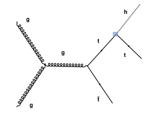
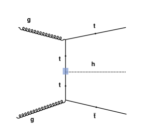
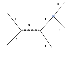
Figure 1: Feynman diagrams contributing to $t\bar{t}h$ production at LO.

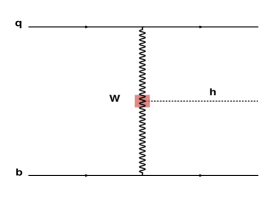
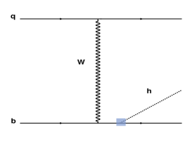
Figure 2: Feynman diagrams contributing to $thX$ production with $X=j$.

As well known $t\bar{t}h$ production only depends on the absolute value of the top-Yukawa coupling at the leading order (LO), see Fig. 1, which is similar to gluon-gluon fusion production. Therefore, the $t\bar{t}h$ cross section is insensitive to the sign of the top-Yukawa coupling at LO. Meanwhile, in $thX$ production, this degeneracy is lifted through the strong interference between the two main contributions, which are proportional to the top-Yukawa and the gauge-Higgs couplings, respectively. Note that we include both $th+X$ and $\bar{t}h+X$ production when we refer to $thX$ with $X$ denoting the accompanied particle(s) produced together with $t(\bar{t})$ and $h$. The Feynman diagrams contributing to $thX$ production with $X=j$ ($qb\to thq^{\prime}$) is depicted in Fig. 2. The left diagram is proportional to the gauge-Higgs coupling while the right one to the top-Yukawa coupling . The interference between the two diagrams was shown to be significant and induces large variations in the total cross section with the size and the relative sign of the Higgs couplings to the gauge bosons and the top quarks. It was shown in literature Chang:2014rfa ; singletop.old ; th-others that the cross section can be enhanced by more than an order of magnitude when the relative sign of the top-Yukawa coupling to the gauge-Higgs coupling is reversed.

In this work, we perform a detailed study of the influence of $thX$ production on $t\bar{t}h$ production in the presence of the anomalous top-Yukawa coupling. While assuming the Standard Model (SM) value for the gauge-Higgs coupling, we vary the top-Yukawa coupling within the allowed range by the current LHC Higgs data. We consider the Higgs decay modes into multileptons , $b\bar{b}$ and $\gamma\gamma$ putting a particular emphasis on the same sign dilepton events. We show that the current ATLAS and CMS analyses of $t\bar{t}h$ could be significantly contaminated by the $thX$ processes. Moreover, the $thX$ processes contribute (or contaminate) at quite different levels in various detection modes of $tth$, depending on the value of top-Yukawa coupling, on the cuts used in each experiment, and on the decay mode of the Higgs boson. We shall illustrate such behavior in Sec. III, which is far more complicated than simply assuming a small constant level of contamination in all channels. In addition to explaining the apparent mild excess in $t\bar{t}h$ production by entangling $thX$ production, we also propose how to disentangle $thX$ production from $t\bar{t}h$ one at the LHC Run-2. The main objective of this work is to further pin down the sign and the size of the top-Yukawa coupling. To achieve the objective, we point out that it is crucial to consider the entanglement between $thX$ and $t\bar{t}h$.

Note that the $\sim 2\sigma$ excesses were seen in the channels of multileptons and $b\bar{b}$ of ATLAS and in the channels of multileptons and $\gamma\gamma$ of CMS, but not in the others. It may as well be due to statistical fluctuations, but could also be due to some specific forms of new physics. Only more data can tell. In this work, we perform a case study in which, through the $thX$ processes, the contributions of the anomalous top-Yukawa coupling to $t\bar{t}h$ production manifest non-trivially depending on the value of top-Yukawa coupling, on the cuts used in each experiment, and on the decay mode of the Higgs. Our case study shows that the (future) observations related to $t\bar{t}h$ production should be carefully made without simply assuming a small constant level of contamination in all channels which is common to both the ATLAS and CMS experiments.

The organization is as follows. In the next section, we lay down the formalism and the calculation method. In Sec. III, we show the influence of $thX$ with the anomalous top-Yukawa coupling on $t\bar{t}h$ for both the ATLAS and CMS Run-1 data. In Sec. IV, we propose some scenarios to further disentangle $thX$ from $t\bar{t}h$ for the LHC Run-2. Finally, we discuss and conclude in Sec. V.

II Formalism

II.1 Processes and Higgs couplings involved

We consider two types of production processes for the Higgs boson and the top quark. The first one is the associated production of the Higgs with a pair of top quarks, see Fig. 1. The second one is the associated Higgs production with a single top quark plus anything else: $thX$ production with $X=j\,(qb\to thq^{\prime}),\ jb\,(qg\to thq^{\prime}b),\ W\,(gb\to thW)$ , see Figs. 2 – 4 in which we have marked the vertices of $hWW$ and $ht\bar{t}$ with squares. In $t\bar{t}h$ production, the production cross section only depends on the square of the top-Yukawa coupling. However, in $thX$ production, the cross sections depend on the size of the gauge-Higgs and top-Yukawa couplings and the relative sign between them.

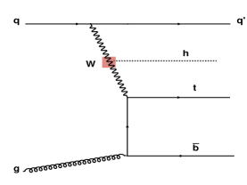
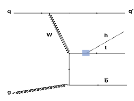
Figure 3: Feynman diagrams contributing to $thX$ production with $X=jb$.

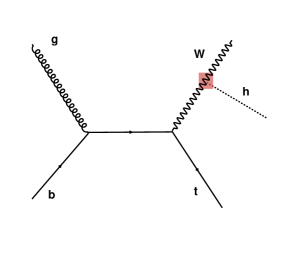
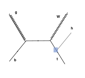
Figure 4: Feynman diagrams contributing to $thX$ production with $X=W$.

In fact, the process $qg\to thjb$ is a part of the NLO QCD corrections to $qb\to thj$ when the momentum of the final $b$ quark in $thjb$ is integrated out. In our work, using MadGraph5@NLO, we calculate the cross section for the $qg\to thjb$ process at NLO adopting the four-flavor scheme. And then, we define $thj$ and $thjb$ productions by introducing a set of separation cuts: $p_{T}^{j}>10$ GeV, $|\eta_{j}|<5$, $p_{T}^{b}>30$ GeV, $|\eta_{b}|<2.5$. Naturally, the low (high) $p_{T}^{b}$ region is taken for $thj$ ($thjb$) production. We obtain $\sigma(thj)=11.2\,(43.0)$ fb and $\sigma(thjb)=5.77\,(23.6)$ fb at the LHC with $\sqrt{s}=8\,(13)$ TeV. We note that the sum $\sigma(thj)+\sigma(thjb)=17.0\,(66.6)$ fb agrees well with the NLO cross sections found in the literature. As will be shown, the contributions of $thj$ and $thjb$ to the accumulated signal strengths strongly depend on the Higgs decay channels and experiment cuts chosen. In this way, we properly reflect the different kinematic signatures of $thj$ and $thjb$ which could be lost if we do not introduce the separation. On the other hand, since the NLO QCD corrections for both $pp\to t\overline{t}h$ and $pp\to thW$ are relatively large compared with $pp\to thj$, we multiply the corresponding $K$ factors to the LO cross sections for each of them.

Without loss of generality, one can write the gauge-Higgs and Yukawa couplings of the Higgs boson $h$ as

$${\cal L}_{hVV} = gm_{W}\left(g_{hWW}W^{+}_{\mu}W^{-\mu}+g_{hZZ}\frac{1}{2c_{W}^{2}}Z_{\mu}Z^{\mu}\right)h\,,$$ (1)

$${\cal L}_{hff} = -\sum_{f=t,b,c,\tau}\,\frac{gm_{f}}{2m_{W}}\,g^{S}_{hff}\,\bar{f}\,f\,h\;.$$ (2)

Here only the gauge-Higgs coupling $g_{hWW}$ and the top-Yukawa couplings are relevant to the $t\bar{t}h$ and $thX$ production processes shown in Figs. 1–4. We note $g_{hWW}=g_{hZZ}=g^{S}_{hff}=1$ in the SM.

In order to calculate the event rates we have to consider the decay branching ratios of the Higgs boson, which depend on $g_{hWW}$, $g_{hZZ}$, $g^{S}_{htt,hbb}$ and a few more couplings, including $h\tau\tau$, $hcc$, $h\gamma\gamma$, and $hgg$. The amplitude for the decay process $h\rightarrow\gamma\gamma$ can be written as

$${\cal M}_{h\gamma\gamma}=-\frac{\alpha m_{h}^{2}}{4\pi\,v}\,S^{\gamma}(m_{h})\,\left(\epsilon^{*}_{1\perp}\cdot\epsilon^{*}_{2\perp}\right)\,,$$ (3)

where $k_{1,2}$ are the momenta of the two photons and $\epsilon_{1,2}$ the wave vectors of the corresponding photons with $\epsilon^{\mu}_{1\perp}=\epsilon^{\mu}_{1}-2k^{\mu}_{1}(k_{2}\cdot\epsilon_{1})/m^{2}_{h}$ and $\epsilon^{\mu}_{2\perp}=\epsilon^{\mu}_{2}-2k^{\mu}_{2}(k_{1}\cdot\epsilon_{2})/m^{2}_{h}$. Retaining only the dominant loop contributions from the third–generation fermions and $W^{\pm}$, and including some additional loop contributions from new particles, the scalar form factor is given by

$$S^{\gamma}(m_{h}) = 2\sum_{f=b,t,\tau}N_{C}\,Q_{f}^{2}\,g^{S}_{hff}\,F_{sf}(\tau_{f})-g_{{}_{hWW}}F_{1}(\tau_{W})+\Delta S^{\gamma}\,,$$ (4)

where $\tau_{x}=m_{h}^{2}/4m_{x}^{2}$, $N_{C}=3$ for quarks and $N_{C}=1$ for tau leptons, respectively. For the loop functions of $F_{sf,1}(\tau)$, we refer to, for example, Ref. Lee:2003nta . The additional contributions $\Delta S^{\gamma}$ are due to additional particles running in the loop. In the SM, $g^{S}_{hff}=g_{hWW}=1$ and $\Delta S^{\gamma}=0$. Similarly, the amplitude for the decay process $h\rightarrow gg$ can be written as

$${\cal M}_{Hgg}=-\frac{\alpha_{s}\,m_{h}^{2}\,\delta^{ab}}{4\pi\,v}\,S^{g}(m_{h})\,\left(\epsilon^{*}_{1\perp}\cdot\epsilon^{*}_{2\perp}\right)\,,$$ (5)

where $a$ and $b$ ($a,b=1$ to 8) are indices of the eight $SU(3)$ generators in the adjoint representation. Including some additional loop contributions from new particles, the scalar form factor is given by

$$S^{g}(m_{h}) = \sum_{f=b,t}g^{S}_{hff}\,F_{sf}(\tau_{f})+\Delta S^{g}\,.$$ (6)

In the SM, $g^{S}_{hff}=1$ and $\Delta S^{g}=0$. In the decays of the Higgs boson, we can see that the partial width into $b\bar{b}$ depends on $g_{hbb}$, that into $WW^{*}$ and $ZZ^{*}$ depends on $g_{hWW,hZZ}$, and that into $\gamma\gamma$ and $gg$ depends implicitly on all $g_{hWW}$, $g_{htt}^{S}$, $g_{hbb}^{S}$, and $g_{h\tau\tau}^{S}$.

The dependence of the production cross sections and the decay branching ratios on $g_{hWW}$ and $g^{S}_{hff}$ has been explicitly shown in the above equations. Since we are primarily interested in size of the gauge-Higgs and top-Yukawa couplings and the relative sign between them, for bookkeeping purpose, we use the following simplified notations

$$C_{v}\equiv g_{hWW}=g_{hZZ}\,,\qquad C^{S}_{t}\equiv g^{S}_{htt}\,,\qquad C^{S}_{b}\equiv g^{S}_{hbb}\,.$$ (7)

We shall show the anomalous top-Yukawa coupling effects on $t\bar{t}h$ and $thX$ production at the LHC in the next section.

II.2 Signal strengths

First we note that signal strengths depend on the decay modes of the top quark and the Higgs boson, as well as their production mechanisms. For a choice of experimentally-defined decay mode ${\cal D}$, and taking into account the $thX$ production processes, we define the signal strength $\mu(t\bar{t}h)$ with respect to the SM $t\bar{t}h$ production as follows

$$\mu(t\bar{t}h)=\frac{\eta_{1}\sigma(t\bar{t}h)B(t\bar{t}h\to{\cal D})+\sum_{X=j,jb,W}\eta_{X}\sigma(thX)B(thX\to{\cal D})}{\eta_{1}^{\rm SM}\sigma(t\bar{t}h)_{\rm SM}B(t\bar{t}h\to{\cal D})_{\rm SM}}\,,$$ (8)

where $\sigma(t\bar{t}h)=\sigma(pp\to t\bar{t}h)$ and $\sigma(thX)=\sigma(pp\to thX)+\sigma(pp\to\bar{t}hX)$ are understood. The detection efficiencies $\eta$’s depend on the experimental apparatuses and cuts for the specific production and decay mode. By introducing the cross-section ratios

$$R(t\bar{t}h)\equiv\frac{\sigma(t\bar{t}h)}{\sigma(t\bar{t}h)_{\rm SM}}\,,\ \ \ R(thj)\equiv\frac{\sigma(thj)}{\sigma(t\bar{t}h)_{\rm SM}}\,,\ \ \$$

$$R(thjb)\equiv\frac{\sigma(thjb)}{\sigma(t\bar{t}h)_{\rm SM}}\,,\ \ \ R(thW)\equiv\frac{\sigma(thW)}{\sigma(t\bar{t}h)_{\rm SM}}\,,$$ (9)

and the ${\cal D}$-dependent detection-efficiency ratios

$$\epsilon_{1}\equiv\frac{\eta_{1}B(t\bar{t}h\to{\cal D})}{\eta_{1}^{\rm SM}B(t\bar{t}h\to{\cal D})_{\rm SM}}\,,\ \ \ \epsilon_{2}\equiv\frac{\eta_{j}B(thj\to{\cal D})}{\eta_{1}^{\rm SM}B(t\bar{t}h\to{\cal D})_{\rm SM}}\,,\ \ \$$

$$\epsilon_{3}\equiv\frac{\eta_{jb}B(thjb\to{\cal D})}{\eta_{1}^{\rm SM}B(t\bar{t}h\to{\cal D})_{\rm SM}}\,,\ \ \ \epsilon_{4}\equiv\frac{\eta_{W}B(thW\to{\cal D})}{\eta_{1}^{\rm SM}B(t\bar{t}h\to{\cal D})_{\rm SM}}\,,$$ (10)

one may have

$$\mu(t\bar{t}h)=\epsilon_{1}\,R(t\bar{t}h)+\epsilon_{2}\,R(thj)+\epsilon_{3}\,R(thjb)+\epsilon_{4}\,R(thW)\,.$$ (11)

We note that $\epsilon_{1}=R(t\bar{t}h)=1$ in the SM limit of $C_{v}=1$ and $C_{t}^{S}=+1$ and $\mu(t\bar{t}h)$ is always larger than $1$ due to the entanglement of $thX$ production. Our main task is to calculate the cross section ratios $R$’s in the presence of anomalous top-Yukawa coupling and the detection-efficiency ratios $\epsilon_{1,2,3,4}$ for various top-quark and Higgs-boson decay modes.

Table 1: The best-fit values for the category-dependent signal strengths $\mu_{tth}^{\rm CMS}$ and $\mu_{tth}^{\rm ATLAS}$ coming from the CMS Khachatryan:2014qaa and ATLAS Aad:2015iha Aad:2014lma Aad:2015gra searches, respectively, for the associated production of the Higgs boson with a top quark pair at $\sqrt{s}$= 7 and 8 TeV for $m_{h}=125.6$ GeV (CMS) / 125 GeV (ATLAS).

	CMS $t\bar{t}h$ channel	ATLAS $t\bar{t}h$ channel
Category	$\mu_{tth}^{\rm CMS}$	$\mu_{tth}^{\rm ATLAS}$
$\gamma\gamma$	$+2.7\,^{+2.6}_{-1.8}$	$+1.3\,^{+3.3}_{-2.1}$
$b\bar{b}$	$+0.7\,^{+1.9}_{-1.9}$	$+1.5\,^{+1.1}_{-1.1}$
$\tau_{h}\tau_{h}$	$-1.3\,^{+6.3}_{-5.5}$	–
$2\ell 1\tau_{h}$	–	$-0.9\,^{+3.1}_{-2.0}$
$1\ell 2\tau_{h}$	–	$-9.6\,^{+9.6}_{-9.7}$
$4\ell$	$-4.7\,^{+5.0}_{-1.3}$	$+1.8\,^{+6.9}_{-2.0}$
$3\ell$	$+3.1\,^{+2.4}_{-2.0}$	$+2.8\,^{+2.2}_{-1.8}$
$ss2\ell$	$+5.3\,^{+2.1}_{-1.8}$	$+2.8\,^{+2.1}_{-1.9}$

III $thX$ production with the anomalous top-Yukawa coupling

Both the CMS Khachatryan:2014qaa and ATLAS Aad:2014lma ; Aad:2015gra ; Aad:2015iha collaborations have published the results of their searches for the associated production of the Higgs boson with a top-quark pair via different Higgs decay channels at $\sqrt{s}$= 7 and 8 TeV. We summarize their best-fit results in Table 1. Since the experimental uncertainties in the hadronically-decaying $\tau$ and $4\ell$ categories are too large at this stage, we shall focus only on the $ss2\ell$, $3\ell$, $\gamma\gamma$ and $b\bar{b}$ categories in our analysis below. In the $\gamma\gamma$ category for $h\to\gamma\gamma$, both CMS Khachatryan:2014qaa and ATLAS Aad:2014lma included all the decay modes of a top-quark pair: semileptonic ($t\bar{t}\rightarrow l\nu jjbb$), leptonic ($t\bar{t}\rightarrow l\nu\l\nu bb$), and hadronic ($t\bar{t}\rightarrow jjjjbb$) modes. On the other hand, in the $b\bar{b}$ category for $h\to b\bar{b}$, both CMS Khachatryan:2014qaa and ATLAS Aad:2015gra considered only the semileptonic and leptonic decay modes of the top-quark pair. Finally, in the categories of $ss2\ell$ and $3\ell$ for $h\rightarrow~{}{\rm multileptons}$, both CMS Khachatryan:2014qaa and ATLAS Aad:2015iha included only the semileptonic decay mode of the top-quark pair.

In order to perform a detailed study of the influence of $thX$ production with anomalous top-Yukawa coupling on $t\bar{t}h$ production, we simulate both the $thX$ and $t\bar{t}h$ processes and generate events by MadGraph5 Alwall:2014hca , perform parton showering and hadronization by Pythia 8.1 Sjostrand:2007gs , and employ the detector simulations by Delphes 3 delphes3 . We use NN23LO1 for parton distribution functions with different renormalization/factorization scales which we shall show below. We follow the selection cuts and detector efficiencies of the CMS Khachatryan:2014qaa and ATLAS Aad:2014lma ; Aad:2015gra ; Aad:2015iha $t\bar{t}h$ searches. We summarize the signatures of the search channels used in the $t\bar{t}h$ analysis for CMS in Table 2 and for ATLAS in Table 3.

Table 2: The signature of the search channels used in the $tth$ analysis for CMS.

Category	$t\overline{t}h$ decay modes	Signature	Background
$h\rightarrow b\overline{b}$	Semileptonic	1 $e/\mu$, $P_{T}>$ 30 GeV	$t\bar{t}+$ jets
	($t\overline{t}h\rightarrow l\nu jjbbbb$)	$\geq$ 4 jets + $\geq$ 2b-tags, $P_{T}>$ 30 GeV	$t\bar{t}+W/Z$
	Leptonic	1 $e/\mu$, $P_{T}>$ 20 GeV	Single $t$
	($t\overline{t}h\rightarrow l\nu l\nu bbbb$)	1 $e/\mu$, $P_{T}>$ 10 GeV	$W/Z+$jets
		$\geq$ 3 jets + $\geq$ 2b-tags, $P_{T}>$ 30 GeV	Diboson
$h\rightarrow\gamma\gamma$	Semileptonic	2$\gamma$, $P_{T}>m_{\gamma\gamma}/2$ (25) GeV for $1^{st}$($2^{nd}$)	$t\bar{t}+$ jets
	($t\overline{t}h\rightarrow l\nu jjbb\gamma\gamma$)	$\geq$ 1 $e/\mu$, $P_{T}>$ 20 GeV	$t\bar{t}+W/Z$
	Leptonic	$\geq$ 2 jets + $\geq$ 1b-tags, $P_{T}>$ 25 GeV	Single $t$
	($t\overline{t}h\rightarrow l\nu l\nu bb\gamma\gamma$)
	Hadronic	2$\gamma$, $P_{T}>m_{\gamma\gamma}/2$ (25) GeV for $1^{st}$($2^{nd}$)
	($t\overline{t}h\rightarrow jjjjbb\gamma\gamma$)	0 $e/\mu$, $P_{T}>$ 20 GeV
		$\geq$ 4 jets + $\geq$ 1b-tags, $P_{T}>$ 25 GeV
$h\rightarrow$ Leptons	Same-Sign Dilepton	2 $e/\mu$, $P_{T}>$ 20 GeV	$t\bar{t}W$
$h\rightarrow WW$	($t\overline{t}h\rightarrow l^{\pm}\nu l^{\pm}[\nu]jjj[j]bb$)	$\geq$ 4 jets + $\geq$ 1b-tags, $P_{T}>$ 25 GeV	$t\bar{t}Z/\gamma^{*}$
$h\rightarrow\tau\tau$	3 Leptons	1 $e/\mu$, $P_{T}>$ 20 GeV	$t\bar{t}WW$
$h\rightarrow ZZ$	($t\overline{t}h\rightarrow l\nu l[\nu]l[\nu]j[j]bb$)	1 $e/\mu$, $P_{T}>$ 10 GeV	$t\bar{t}\gamma$
		1 $e(\mu)$, $P_{T}>$ 7(5) GeV	$WZ$
		$\geq$ 2 jets + $\geq$ 1b-tags, $P_{T}>$ 25 GeV	$ZZ$

Table 3: The signature of the search channels used in the $tth$ analysis for ATLAS.

Category	$t\overline{t}h$ decay modes	Signature	Background
$h\rightarrow b\overline{b}$	Semileptonic	1 $e/\mu$, $P_{T}>$ 25 GeV, $\bigtriangleup R<$ 0.15	$t\bar{t}+$jets
	($t\overline{t}h\rightarrow l\nu jjbbbb$)	$\geq$ 4 jets + $\geq$ 2b-tags	$t\bar{t}+V$
	Leptonic	1 $e/\mu$, $P_{T}>$ 25 GeV	$V+$jets
	($t\overline{t}h\rightarrow l\nu l\nu bbbb$)	1 $e/\mu$, $P_{T}>$ 15 GeV	($V=W,Z$)
		$\geq$ 2b-tags
$h\rightarrow\gamma\gamma$	Semileptonic	2$\gamma$, $E_{T}>0.35(0.25)\times m_{\gamma\gamma}$ for $1^{st}$($2^{nd}$)
	($t\overline{t}h\rightarrow l\nu jjbb\gamma\gamma$)	$\geq$ 1 $e/\mu$, $E_{T}(e)>$ 15 GeV, $P_{T}(\mu)>$ 10 GeV
	Leptonic	$\geq$ 1 b-tags
	($t\overline{t}h\rightarrow l\nu l\nu bb\gamma\gamma$)
	Hadronic	2$\gamma$, $E_{T}>0.35(0.25)\times m_{\gamma\gamma}$ for $1^{st}$($2^{nd}$)
	($t\overline{t}h\rightarrow jjjjbb\gamma\gamma$)	0 $e/\mu$
		$\geq$ 5 jets + $\geq$ 1 b-tags, $P_{T}>$ 25 GeV
$h\rightarrow$ Leptons	Same-Sign Dilepton	(sub)leading lepton : 2 $e/\mu$, $P_{T}>$ 25(20) GeV	$t\bar{t}+$jets
$h\rightarrow WW$	($t\overline{t}h\rightarrow l^{\pm}\nu l^{\pm}[\nu]jjj[j]bb$)	$\geq$ 4 jets + $\geq$ 1b-tags, $P_{T}>$ 25 GeV	$t\bar{t}+V$
$h\rightarrow\tau\tau$	3 Leptons	1 $e/\mu$, $P_{T}>$ 25 GeV	Diboson
$h\rightarrow ZZ$	($t\overline{t}h\rightarrow l\nu l[\nu]l[\nu]j[j]bb$)	1 $e/\mu$, $P_{T}>$ 20 GeV
		1 $e/\mu$, $P_{T}>$ 10 GeV
		$\geq$ 4 jets + $\geq$ 1 b-tags, $P_{T}>$ 25 GeV
		(or 3 jets + $\geq$ 2 b-tags, $P_{T}>$ 25 GeV )

We calculate the $t\bar{t}h$ production cross section with the factorization ($\mu_{F}$) and renormalization ($\mu_{R}$) scales set at $m_{t}+m_{h}/2$ in the four-flavor scheme. On the other hand, in computing the production cross sections for $thX$, we include the $t$-channel $thj$ and $thjb$ processes and the $thW$ process, but ignore the $s$-channel $thb$ process due to its much smaller cross section. In calculating the production cross sections for $thj$ and $thjb$, $\mu_{F}=\mu_{R}$ are set at $75$ GeV in the four-flavor scheme. For $thW$, we are employing the dynamic factorization and renormalization scales in the five-flavor scheme.

As shown in Refs. higgcision in which the model-independent fit to the current Higgs data is performed, the negative $C^{S}_{t}=-1$ is ruled at 95%CL if only the gauge-Higgs coupling $C_{v}$ and the top-Yukawa coupling $C^{S}_{t}$ vary. However, $C^{S}_{t}=-1$ is still allowed at 95%CL when the gauge-Higgs $C_{v}$, top-Yukawa $C^{S}_{t}$, bottom-Yukawa $C^{S}_{b}$, and tau-Yukawa $C^{S}_{\tau}$ couplings are all allowed to vary. Furthermore, if some sizable contributions to $\Delta S^{\gamma}$ and $\Delta S^{g}$ due to additional new particles running in the loop are assumed, a broad range of $C_{t}^{S}$ between $-2$ and $+2$ is still consistent with the current Higgs data.

In the following, we show the results of our numerical analysis in each of categories of Leptons ($ss2\ell$ and $3\ell$), $\gamma\gamma$, and $b\bar{b}$ for the Higgs boson decaying into multileptons, two photons, and two $b$ quarks, respectively. Note that, in our numerical analysis, we vary the top-Yukawa coupling $C_{t}^{S}$ within the range allowed by the current LHC Higgs data while taking the SM value for the gauge-Higgs coupling, $C_{v}=1$. For the bottom-Yukawa $C^{S}_{b}$ and tau-Yukawa $C^{S}_{\tau}$ couplings, one may freely take either $+1$ or $-1$ since their signs would have negligible effects on the production cross sections and decay branching ratios.

III.1 Category Leptons for $h\rightarrow$ multileptons

In the category Leptons which includes leptonic decays of $h\rightarrow WW,ZZ,\tau\tau\to$ multileptons, we focus on the subcategories of $ss2\ell$ and $3\ell$ modes. We shall use several different values of $C^{S}_{t}$ to show the possibly strong entanglement between $thX$ production and $t\bar{t}h$ production for both the ATLAS and CMS analyses. Note that CMS used the so-called Multivariate Analysis (MVA) method in their analysis, however, we only follow their set of preselection cuts and event selection requirements to perform the cut-based analysis.

First, we note that the CMS and ATLAS collaborations were adopting different signatures and preselection cuts to analyze the category Leptons as shown in Table 2 and Table 3 . The CMS analysis was performed in the $ss2\ell$ and $3\ell$ subcategories while the ATLAS analysis was carried out in the subcategories of $2\ell+4j$, $2\ell+\geq 5j$, and $3\ell$. Without knowing an appropriate way to combine the two sets of data, we present our results handling the CMS and ATLAS cases separately to make full use of the existing data. Further, in the CMS and ATLAS analyses of the $3\ell$ subcategory, also required was a low-mass invariant-mass cut $M_{\ell\ell}>12$ GeV to remove the $J/\Psi$ background and a $Z$-pole mass veto cut $|M_{\ell^{+}\ell^{-}}-M_{Z}|>10$ GeV to suppress the $Z$ background. Some additional cuts on the scalar sum of the transverse momenta ($P_{T}$) of the two leptons and the missing energy ($E_{T}^{\rm miss}$) were also applied in the CMS case.

To quantify the effects of different values of $C^{S}_{t}$ on $t\bar{t}h$ and $thX$, we use the signal-strength formula for $\mu(t\bar{t}h)$ in Eq. (8), which consists of the sum of the products of the cross section ratios $R$’s and the ${\cal D}$-dependent detection efficiency ratio $\epsilon$’s, which are in turns given by Eq. (9) and Eq. (10), respectively. Explicitly, we have

$$\mu(t\bar{t}h) = \frac{\sigma(t\bar{t}h)_{C^{S}_{t}}}{\sigma(t\bar{t}h)_{SM}}\times\epsilon_{1}+\frac{\sigma(thj)_{C^{S}_{t}}}{\sigma(t\bar{t}h)_{SM}}\times\epsilon_{2}+\frac{\sigma(thjb)_{C^{S}_{t}}}{\sigma(t\bar{t}h)_{SM}}\times\epsilon_{3}+\frac{\sigma(thW)_{C^{S}_{t}}}{\sigma(t\bar{t}h)_{SM}}\times\epsilon_{4}\,$$ (12)

$$= R(t\bar{t}h)\times\epsilon_{1}+R(thj)\times\epsilon_{2}+R(thjb)\times\epsilon_{3}+R(thW)\times\epsilon_{4}\,.$$

Table 4: The cross-section ratios $R(t\bar{t}h)$ and $R(thX)$ with $X=j,jb,W$ defined in Eq. (9). We are taking $\sqrt{s}=8$ TeV (LHC-8) and $C_{t}^{S}=\pm 1\,,\pm 1.5$.

LHC-8	$C^{S}_{t}=1$	$C^{S}_{t}=-1$	$C^{S}_{t}=1.5$	$C^{S}_{t}=-1.5$
Cross Section of $t\bar{t}h$(pb)	0.13
$R(t\bar{t}h)$	1	1	2.25	2.25
$R(thj)$	8.36e-2	1.08	0.15	1.66
$R(thjb)$	4.30e-2	0.54	8.56e-2	0.84
$R(thW)$	3.21e-2	0.19	7.05e-2	0.31

In Table 4, we show the cross section ratios $R(t\bar{t}h)$ and $R(thX)$ with $X=j,jb,W$ at the 8 TeV LHC (LHC-8) taking $C_{t}^{S}=\pm 1$ and $\pm 1.5$. Note $R(t\bar{t}h)=1\,(2.25)$ for $|C_{t}^{S}|=1\,(1.5)$ and the $thX$ cross sections can be largely enhanced for the negative values of $C_{t}^{S}$.

In Table 5, we show the ${\cal D}$-dependent detection efficiency ratios $\epsilon_{1,2,3,4}$ with the CMS cuts in the $ss2\ell$ (upper) and $3\ell$ (lower) subcategories for $C_{t}^{S}=\pm 1\,,\pm 1.5$. By using the cross section ratios given in Table 4, one can obtain the CMS $t\bar{t}h$ signal strengths $\mu_{tth}^{\rm CMS}$. We observe that $\mu_{tth\,,ss2\ell}^{\rm CMS}\sim 2\,(3)$ for $C_{t}^{S}=1.5\,(-1.5)$ and the signal strengths are larger for the negative values of $C_{t}^{S}$. One may make similar observations for $\mu_{tth\,,3\ell}^{\rm CMS}$. Recently, the CMS collaboration has also reported a possible excess in the decay process $h\rightarrow\tau^{\mp}\mu^{\pm}$, $B(h\rightarrow\tau^{\mp}\mu^{\pm})=0.84\,^{+0.39}_{-0.37}\%$, with a significance of $2.4\sigma$ in the search for the lepton-flavor violation (LFV)Khachatryan:2015kon . If we take into account this LFV decay of the Higgs boson, we can slightly enhance the production rate of $h\rightarrow$ multileptons mode by a few percents. We estimate the $h\rightarrow\tau^{\mp}\mu^{\pm}$ contribution by rescaling $h\rightarrow\tau^{+}\tau^{-}$ channel with the branching ratios and the $\tau$ detection efficiency. The CMS $t\bar{t}h$ signal strengths $\mu_{tth}^{\rm CMS}$ after taking account of $h\rightarrow\tau^{\mp}\mu^{\pm}$ are also presented in Table 5.

Table 5: Category Leptons: The ${\cal D}$-dependent detection efficiency ratios $\epsilon_{i}$’s defined in Eq. (10) with the CMS cuts for the category Leptons taking $C_{t}^{S}=\pm 1\,,\pm 1.5$ and $\sqrt{s}=8$ TeV. The resulting signal strengths $\mu_{tth\,,ss2\ell}^{\rm CMS}$ and $\mu_{tth\,,3\ell}^{\rm CMS}$ are also shown. The last row in each partition shows the values of $\mu_{tth\,,ss2\ell}^{\rm CMS}$ and $\mu_{tth\,,3\ell}^{\rm CMS}$ including the contributions from $h\to\mu^{\pm}\tau^{\mp}$.

LHC-8	With CMS Analysis Cuts
	$C^{S}_{t}=1$	$C^{S}_{t}=-1$	$C^{S}_{t}=1.5$	$C^{S}_{t}=-1.5$
	The category of $ss2\ell$
Efficiency of $t\bar{t}h$	9.02e-4
$\epsilon_{1}$	1	0.95	0.98	0.97
$\epsilon_{2}$	0.1	0.12	0.12	0.13
$\epsilon_{3}$	0.35	0.38	0.33	0.39
$\epsilon_{4}$	0.68	0.85	0.72	0.83
$\mu_{tth\,,ss2\ell}^{\rm CMS}$	1.05	1.45	2.31	2.99
$\mu_{tth\,,ss2\ell}^{\rm CMS}$ including $h\rightarrow\tau^{\mp}\mu^{\pm}$	1.09	1.51	2.40	3.11
	The category of $3\ell$
Efficiency of $t\bar{t}h$	9.54e-4
$\epsilon_{1}$	1	0.95	1	0.97
$\epsilon_{2}$	0.34	0.40	0.37	0.42
$\epsilon_{3}$	0.55	0.61	0.57	0.65
$\epsilon_{4}$	0.90	1.14	0.98	1.13
$\mu_{tth\,,3\ell}^{\rm CMS}$	1.08	1.93	2.42	3.77
$\mu_{tth\,,3\ell}^{\rm CMS}$ including $h\rightarrow\tau^{\mp}\mu^{\pm}$	1.12	2.01	2.51	3.92

Similarly, we calculate the ${\cal D}$-dependent detection efficiency ratios $\epsilon_{1,2,3,4}$ with the ATLAS cuts in the $2\ell+4j$ (upper), $2\ell+\geq 5j$ (middle), and $3\ell$ (lower) subcategories for several values of $C_{t}^{S}$ and present them in Table 6, together with the ATLAS $t\bar{t}h$ signal strengths $\mu_{tth}^{\rm ATLAS}$. Similar observations can be made as in the CMS case.

Table 6: Category Leptons: The same as Table 5 but with the ATLAS cuts.

LHC-8	With ATLAS Analysis Cuts
	$C^{S}_{t}=1$	$C^{S}_{t}=-1$	$C^{S}_{t}=1.5$	$C^{S}_{t}=-1.5$
	The category of $2\ell+4j$
Efficiency of $t\bar{t}h$	4.27e-4
$\epsilon_{1}$	1	1.05	0.96	1.0
$\epsilon_{2}$	0.31	0.31	0.32	0.38
$\epsilon_{3}$	0.52	0.63	0.53	0.57
$\epsilon_{4}$	1.10	1.16	1.09	1.18
$\mu_{tth\,,2\ell+4j}^{\rm ATLAS}$	1.08	1.96	2.33	3.72
$\mu_{tth\,,2\ell+4j}^{\rm ATLAS}$ including $h\rightarrow\tau^{\mp}\mu^{\pm}$	1.13	2.03	2.42	3.86
	The category of $2\ell+\geq 5j$
Efficiency of $t\bar{t}h$	5.25e-4
$\epsilon_{1}$	1	0.92	0.91	0.93
$\epsilon_{2}$	0.08	0.08	0.09	0.09
$\epsilon_{3}$	0.25	0.28	0.22	0.26
$\epsilon_{4}$	0.74	0.94	0.75	0.95
$\mu_{tth\,,2\ell+\geq 5j}^{\rm ATLAS}$	1.04	1.35	2.13	2.74
$\mu_{tth\,,2\ell+\geq 5j}^{\rm ATLAS}$ including $h\rightarrow\tau^{\mp}\mu^{\pm}$	1.08	1.40	2.22	2.85
	The category of $3\ell$
Efficiency of $t\bar{t}h$	1.05e-4
$\epsilon_{1}$	1	0.89	0.83	0.90
$\epsilon_{2}$	0.06	0.09	0.13	0.09
$\epsilon_{3}$	0.34	0.45	0.30	0.47
$\epsilon_{4}$	0.89	1.5	0.92	1.61
$\mu_{tth\,,3\ell}^{\rm ATLAS}$	1.05	1.52	1.97	3.07
$\mu_{tth\,,3\ell}^{\rm ATLAS}$ including $h\rightarrow\tau^{\mp}\mu^{\pm}$	1.09	1.58	2.05	3.19

Finally, we show in Fig. 5 the accumulative signal strengths $\mu_{tth\,,ss2\ell}^{\rm ATLAS}$ (upper left), $\mu_{tth\,,3\ell}^{\rm ATLAS}$ (upper right), $\mu_{tth\,,ss2\ell}^{\rm CMS}$ (lower left), and $\mu_{tth\,,3\ell}^{\rm CMS}$ (lower right) at $\sqrt{s}=8$ TeV by stacking the various $thX$ contributions on the $t\bar{t}h$ one for $C_{t}^{S}=+1\,,-1\,,+1.5\,,-1.5$ from left to right. The grey columns in the center without $C_{t}^{S}$ value represent the current 8 TeV LHC data, see Table 1. The ATLAS $ss2\ell$ signal strength $\mu_{tth\,,ss2\ell}^{\rm ATLAS}$ is obtained by counting the event rates by combining the $2\ell+4j$ and $2\ell+\geq 5j$ selections.

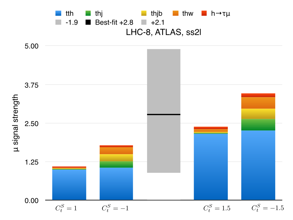
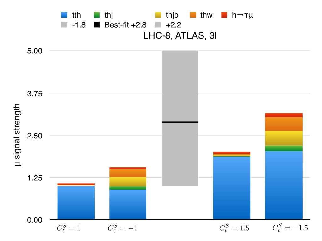
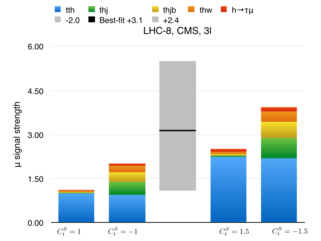
Figure 5: Category Leptons: Accumulated signal strengths $\mu_{tth\,,ss2\ell}^{\rm ATLAS}$ (upper left), $\mu_{tth\,,3\ell}^{\rm ATLAS}$ (upper right), $\mu_{tth\,,ss2\ell}^{\rm CMS}$ (lower left), and $\mu_{tth\,,3\ell}^{\rm CMS}$ (lower right) at LHC-8 obtained by stacking the various $thX$ contributions on the $t\bar{t}h$ one for $C_{t}^{S}=+1\,,-1\,,+1.5\,,-1.5$ from left to right. The grey columns in the center represent the current 8 TeV LHC data from Table 1.

Table 7: Category $\gamma\gamma$: The ${\cal D}$-dependent detection efficiency ratios $\epsilon_{i}$’s defined in Eq. (10) with the CMS cuts for the category $\gamma\gamma$ taking $C_{t}^{S}=\pm 1\,,\pm 1.5$ and $\sqrt{s}=8$ TeV. The resulting signal strengths $\mu_{tth\,,\gamma\gamma(lep)}^{\rm CMS}$ and $\mu_{tth\,,\gamma\gamma(had)}^{\rm CMS}$ are also shown. Note that the CMS cuts $N(j)\geq 4,N(b)\geq 1$ for $\gamma\gamma$ hadronic channel are not strong enough to separate $t\bar{t}h$ from $thX$ processes.

LHC-8	With CMS Analysis Cuts
	$C^{S}_{t}=1$	$C^{S}_{t}=-1$	$C^{S}_{t}=1.5$	$C^{S}_{t}=-1.5$
	Leptonic Selection
Efficiency of $t\bar{t}h$	1.13e-5
$\epsilon_{1}$	1	0.81	0.99	0.92
$\epsilon_{2}$	0.03	0.02	0.01	0.02
$\epsilon_{3}$	0.11	0.10	0.08	0.10
$\epsilon_{4}$	0.57	0.86	0.83	0.76
$\mu_{tth\,,\gamma\gamma(lep)}^{\rm CMS}$	1.03	1.05	2.29	2.42
	Hadronic Selection
Efficiency of $t\bar{t}h$	1.47e-4
$\epsilon_{1}$	1	0.99	1.05	0.97
$\epsilon_{2}$	0.44	0.47	0.43	0.50
$\epsilon_{3}$	1.40	1.62	1.47	1.58
$\epsilon_{4}$	0.52	0.65	0.54	0.68
$\mu_{tth\,,\gamma\gamma(had)}^{\rm CMS}$	1.11	2.50	2.59	4.56
Combined $\mu_{tth\,,\gamma\gamma}^{\rm CMS}$	1.11	2.40	2.57	4.41

Table 8: Category $\gamma\gamma$: The same as Table 7 with the ATLAS cuts.

LHC-8	With ATLAS Analysis Cuts
	$C^{S}_{t}=1$	$C^{S}_{t}=-1$	$C^{S}_{t}=1.5$	$C^{S}_{t}=-1.5$
	Leptonic Selection
Efficiency of $t\bar{t}h$	8.15e-6
$\epsilon_{1}$	1.00	0.69	0.96	1.19
$\epsilon_{2}$	0.03	0.08	0.11	0.06
$\epsilon_{3}$	0.14	0.11	0.06	0.11
$\epsilon_{4}$	0.82	0.74	1.06	0.43
$\mu_{tth\,,\gamma\gamma(lep)}^{\rm ATLAS}$	1.03	0.99	2.25	3.01
	Hadronic Selection
Efficiency of $t\bar{t}h$	1.06e-4
$\epsilon_{1}$	1	1.01	1.03	0.98
$\epsilon_{2}$	0.05	0.05	0.05	0.07
$\epsilon_{3}$	0.39	0.46	0.44	0.46
$\epsilon_{4}$	0.39	0.49	0.38	0.48
$\mu_{tth\,,\gamma\gamma(had)}^{\rm ATLAS}$	1.03	1.40	2.39	2.85
Combined $\mu_{tth\,,\gamma\gamma}^{\rm ATLAS}$	1.03	1.37	2.38	2.86

III.2 Category $\gamma\gamma$ for $h\rightarrow$ $\gamma\gamma$

In the category $\gamma\gamma$ for $h\rightarrow$ $\gamma\gamma$, we include all the decay modes of the top-quark pair. We consider two subcategories of leptonic selection and hadronic selection. The lepton-selection subcategory is for the semileptonically and leptonically decaying top-quark pair while the hadronic-selection one for the hadronically decaying top-quark pair. To single out the effect of anomalous top-Yukawa coupling on $thj$ and $tth$ production in this category, we assume a non-vanishing $\Delta S^{\gamma}$ due to additional particles running in the $h$-$\gamma$-$\gamma$ loop, see Eq. (4). In fact, one may have $B(h\rightarrow\gamma\gamma)=(2.3,5.4,1.53,5.68)\times 10^{-3}$ for $C^{S}_{t}=(1,\ -1,\ 1.5,\ -1.5)$ using, for example, HDECAY hdecay . We are using $B(h\rightarrow\gamma\gamma)=2.3\times 10^{-3}$ independently of $C_{t}^{S}$ assuming a non-zero $\Delta S^{\gamma}$ which cancels out the the effect of anomalous top-Yukawa coupling on $B(h\rightarrow\gamma\gamma)$. This assumption also helps to avoid the constraint on $S^{\gamma}(m_{h})$ from the current LHC Higgs data higgcision .

To repeat the CMS analysis, we follow their selection cuts listed in Table 2, which are used in the cut-based analysis Khachatryan:2014qaa . Also, we further impose the Higgs-mass window cut: $100\,{\rm GeV}\leq m_{\gamma\gamma}\leq 180$ GeV.

For the ATLAS analysis, we follow Ref. Aad:2014lma with preselection cuts listed in Table 3. We further impose the Higgs-mass window cut ($105\,{\rm GeV}<m_{\gamma\gamma}<160\,{\rm GeV}$) and the $\Delta R$ cuts: $\Delta R_{l\gamma}>0.4$, $\Delta R_{j\gamma}>0.4$, $\Delta R_{j\mu}>0.4$, $\Delta R_{je}>0.2$. The missing energy cut $E_{T}^{miss}>20$ GeV and the $e\gamma$ invariant-mass cut $M_{e\gamma}>94\,{\rm GeV}$ or $<84\,{\rm GeV}$ are also applied in the leptonic-selection category. In the hadronic-selection subcategory, we adopt the selection 1 in Ref. Aad:2014lma using the working point with efficiency of $70\%$ for identifying $b$-jets.

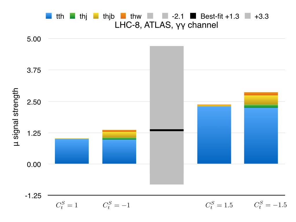
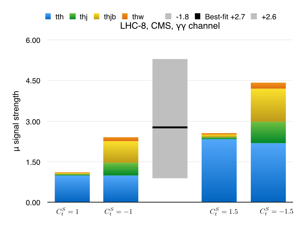
Figure 6: Category $\gamma\gamma$: Accumulated signal strengths $\mu_{tth\,,\gamma\gamma}^{\rm ATLAS}$ (left) and $\mu_{tth\,,\gamma\gamma}^{\rm CMS}$ (lower right) at LHC-8 obtained by stacking the various $thX$ contributions on the $t\bar{t}h$ one for $C_{t}^{S}=+1\,,-1\,,+1.5\,,-1.5$ from left to right. The grey columns in the center represent the current 8 TeV LHC data from Table 1.

Before we present the results of our numerical study of the effects of $thX$ on $t\bar{t}h$ in the category $\gamma\gamma$, we would like to make some remarks on a few noticeable aspects from the ATLAS $t\bar{t}h$ search. It has been shown that there was no significant excess over the background in the $h\to\gamma\gamma$ mode, and thus the 95% CL upper limit is set at $6.7\times\sigma_{\rm SM}(t\bar{t}h)$. Especially, ATLAS took into account the dependence of the $t\bar{t}h$ and $thX$ cross sections as well as the branching ratio $B(h\rightarrow\gamma\gamma)$ on the top-Yukawa coupling. The ATLAS $t\bar{t}h$ search sets the lower and upper limits on $C_{t}^{S}$: $-1.3\leq C_{t}^{S}\leq 8.0$ at 95% CL.

In Table 7, we show the ${\cal D}$-dependent detection efficiency ratios $\epsilon_{1,2,3,4}$ with the CMS cuts in the hadronic-selection (upper) and leptonic-selection (lower) subcategories for $C_{t}^{S}=\pm 1\,,\pm 1.5$. By using the cross section ratios given in Table 4, one can obtain the CMS $t\bar{t}h$ signal strengths $\mu_{tth\,,\gamma\gamma(lep)}^{\rm CMS}$ and $\mu_{tth\,,\gamma\gamma(had)}^{\rm CMS}$ using Eq. (12). In the leptonic-selection subcategory, we observe that $\mu_{tth\,,\gamma\gamma(lep)}^{\rm CMS}>2$ for $|C_{t}^{S}|=1.5$. In the hadronic-selection subcategory, we obtain the larger values for negative $C_{t}^{S}$: $\mu_{tth\,,\gamma\gamma(had)}^{\rm CMS}\sim 1,\ 2.5;\ 2.5,\ 5$ for $C^{S}_{t}=(+1,\ -1;\ +1.5\ -1.5)$. Also presented is the combined signal strength $\mu_{tth\,,\gamma\gamma}^{\rm CMS}$ which is obtained by counting the event rates by combining the hadronic and leptonic selections. Similarly, in Table 8, we show the ${\cal D}$-dependent detection efficiency ratios $\epsilon_{1,2,3,4}$ with the ATLAS cuts and the signal strengths $\mu_{tth\,,\gamma\gamma(lep)}^{\rm ATLAS}$, $\mu_{tth\,,\gamma\gamma(had)}^{\rm ATLAS}$, and $\mu_{tth\,,\gamma\gamma}^{\rm ATLAS}$. Similar observations can be made as in the CMS case.

Finally, in Fig. 6, we show the accumulative combined signal strengths $\mu_{tth\,,\gamma\gamma}^{\rm ATLAS}$ (left) and $\mu_{tth\,,\gamma\gamma}^{\rm CMS}$ (right) at $\sqrt{s}=8$ TeV by stacking the various $thX$ contributions on the $t\bar{t}h$ one for $C_{t}^{S}=+1\,,-1\,,+1.5\,,-1.5$ from left to right. The grey columns in the center without $C_{t}^{S}$ value represent the current 8 TeV LHC data, see Table 1.

Table 9: Category $b\bar{b}$: The ${\cal D}$-dependent detection efficiency ratios $\epsilon_{i}$’s defined in Eq. (10) with the CMS cuts for the category $b\bar{b}$ taking $C_{t}^{S}=\pm 1\,,\pm 1.5$ and $\sqrt{s}=8$ TeV. The resulting signal strengths $\mu_{tth\,,b\bar{b}(1\ell)}^{\rm CMS}$ and $\mu_{tth\,,b\bar{b}(2\ell)}^{\rm CMS}$ and the combined one $\mu_{tth\,,b\bar{b}}^{\rm CMS}$ are also shown.

LHC-8	With CMS Analysis Cuts
	$C^{S}_{t}=1$	$C^{S}_{t}=-1$	$C^{S}_{t}=1.5$	$C^{S}_{t}=-1.5$
	Single Lepton
Efficiency of $t\bar{t}h$	1.17e-1
$\epsilon_{1}$	1	1	0.98	1
$\epsilon_{2}$	0.39	0.42	0.38	0.41
$\epsilon_{3}$	0.67	0.69	0.69	0.70
$\epsilon_{4}$	0.81	0.89	0.82	0.89
$\mu_{tth\,,b\bar{b}(1\ell)}^{\rm CMS}$	1.09	2.01	2.38	3.79
	Dilepton
Efficiency of $t\bar{t}h$	2.03e-2
$\epsilon_{1}$	1	1.09	1.04	0.99
$\epsilon_{2}$	0.14	0.18	0.17	0.17
$\epsilon_{3}$	0.33	0.37	0.33	0.36
$\epsilon_{4}$	0.73	0.87	0.77	0.80
$\mu_{tth\,,b\bar{b}(2\ell)}^{\rm CMS}$	1.05	1.66	2.45	3.05
Combined $\mu_{tth\,,b\bar{b}}^{\rm CMS}$	1.08	1.96	2.39	3.68

Table 10: Category $b\bar{b}$: The same as Table 9 but with the ATLAS cuts.

LHC-8	With ATLAS Analysis Cuts
	$C^{S}_{t}=1$	$C^{S}_{t}=-1$	$C^{S}_{t}=1.5$	$C^{S}_{t}=-1.5$
	Single Lepton
Efficiency of $t\bar{t}h$	1.19e-1
$\epsilon_{1}$	1	1.01	0.99	0.99
$\epsilon_{2}$	0.36	0.40	0.40	0.42
$\epsilon_{3}$	0.66	0.68	0.69	0.69
$\epsilon_{4}$	0.78	0.88	0.80	0.88
$\mu_{tth\,,b\bar{b}(1\ell)}^{\rm ATLAS}$	1.08	1.98	2.40	3.78
	Dilepton
Efficiency of $t\bar{t}h$	1.57e-2
$\epsilon_{1}$	1	1.02	1.07	0.95
$\epsilon_{2}$	0.07	0.08	0.06	0.08
$\epsilon_{3}$	0.11	0.13	0.11	0.11
$\epsilon_{4}$	0.86	0.86	0.86	0.86
$\mu_{tth\,,b\bar{b}(2\ell)}^{\rm ATLAS}$	1.04	1.35	2.50	2.63
Combined $\mu_{tth\,,b\bar{b}}^{\rm ATLAS}$	1.08	1.91	2.41	3.64

III.3 Category $b\bar{b}$ for $h\rightarrow$ $b\bar{b}$

In the category $b\bar{b}$ for $h\rightarrow$ $b\bar{b}$, we consider the semileptonic and leptonic decay modes of the top-quark pair which leads to the two subcategories of single lepton ($1\ell$) and dilepton ($2\ell$). The CMS preselection cuts shown in Table 2 and the ATLAS ones in Table 3 are first applied. And we further impose $P_{T_{j}}>40$ GeV for the leading 3 jets in the single-lepton subcategory. In the dilepton subcategory, we select the events with exactly two oppositely charged leptons $e^{+}e^{-},e^{\pm}\mu^{\mp},\mu^{+}\mu^{-}$ with $P_{T_{l_{1}}}>25$ GeV and $P_{T_{l_{2}}}>15$ GeV. For $e^{\pm}\mu^{\mp}$ events, we further require $H_{T}$, scalar sum of transverse momenta of leptons and jets, to be larger than $130$ GeV. For $e^{+}e^{-}$ and $\mu^{+}\mu^{-}$ events, we impose two more conditions: (i) more than 2 $b$-jets and $M_{ll}>15$ GeV to reduce the $J/\Psi$ background and (ii) exactly 2 $b$-jets, $M_{ll}>60$ GeV to remove the events in the low-mass region with large error bars, and $|M_{ll}-M_{Z}|>8$ GeV to veto the $Z$ background. We then combine these selections to complete the dilepton selection.

In Table 9, we show the ${\cal D}$-dependent detection efficiency ratios $\epsilon_{1,2,3,4}$ with the CMS cuts in the single-lepton (upper) and dilepton (lower) subcategories for $C_{t}^{S}=\pm 1\,,\pm 1.5$. By using the cross section ratios given in Table 4, one can obtain the CMS $t\bar{t}h$ signal strengths $\mu_{tth\,,b\bar{b}(1\ell)}^{\rm CMS}$ and $\mu_{tth\,,b\bar{b}(2\ell)}^{\rm CMS}$ using Eq. (12). We observe that $\mu_{tth\,,b\bar{b}(1\ell)}^{\rm CMS}>2$ for $C_{t}^{S}=-1\,,\pm 1.5$ and $\mu_{tth\,,b\bar{b}(2\ell)}^{\rm CMS}>2$ for $C_{t}^{S}=\pm 1.5$. The combined signal strength $\mu_{tth\,,b\bar{b}}^{\rm CMS}\>\raisebox{-2.15277pt}{$\stackrel{{\scriptstyle\textstyle>}}{{\sim}}$}\>2$ for $C_{t}^{S}=-1\,,\pm 1.5$.

Similarly, in Table 10, we show the ${\cal D}$-dependent detection efficiency ratios $\epsilon_{1,2,3,4}$ with the ATLAS cuts and the signal strengths $\mu_{tth\,,b\bar{b}(1\ell)}^{\rm ATLAS}$, $\mu_{tth\,,b\bar{b}(2\ell)}^{\rm ATLAS}$, and $\mu_{tth\,,b\bar{b}}^{\rm ATLAS}$. Similar observations can be made as in the CMS case.

Finally, we show in Fig. 7 the accumulative combined signal strengths $\mu_{tth\,,b\bar{b}}^{\rm ATLAS}$ (left) and $\mu_{tth\,,\bar{b}}^{\rm CMS}$ (right) at $\sqrt{s}=8$ TeV by stacking the various $thX$ contributions on the $t\bar{t}h$ one for $C_{t}^{S}=+1\,,-1\,,+1.5\,,-1.5$ from left to right. The grey columns in the center without $C_{t}^{S}$ value represent the current 8 TeV LHC data, see Table 1.

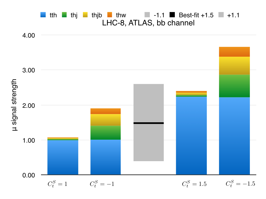
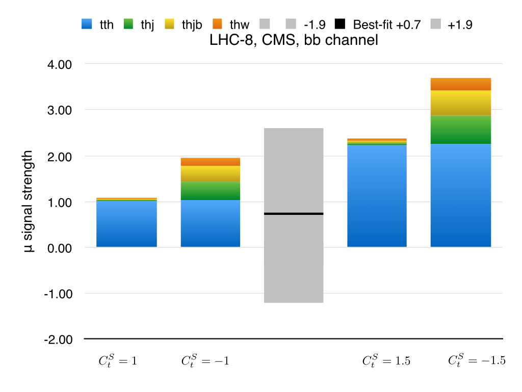
Figure 7: Category $b\bar{b}$: Accumulated signal strengths $\mu_{tth\,,b\bar{b}}^{\rm ATLAS}$ (left) and $\mu_{tth\,,b\bar{b}}^{\rm CMS}$ (lower right) at LHC-8 obtained by stacking the various $thX$ contributions on the $t\bar{t}h$ one for $C_{t}^{S}=+1\,,-1\,,+1.5\,,-1.5$ from left to right. The grey columns in the center represent the current 8 TeV LHC data from Table 1.

Before closing this section, we would like to make a comment on the 13 TeV data on $\mu_{tth}$. With $13.3$ fb^-1 at 13 TeV, ATLAS gives atlas-tth-13 :

$$\mu^{\rm ATLAS}_{tth,multileptons}=2.5^{+1.3}_{-1.1}\,;\ \ \ \mu^{\rm ATLAS}_{tth,\gamma\gamma}=-0.3^{+1.2}_{-1.0}\,;\ \ \ \mu^{\rm ATLAS}_{tth,bb}=2.1^{+1.0}_{-0.9}$$

leading to the combined value of $\mu^{\rm ATLAS}_{tth,combined}=1.8^{+0.7}_{-0.7}$. While, with $12.9$ fb^-1 at 13 TeV, CMS gives cms-tth-13 :

$$\mu^{\rm CMS}_{tth,multileptons}=2.3^{+0.9}_{-0.8}\,;\ \ \ \mu^{\rm CMS}_{tth,\gamma\gamma(lep)}=1.15^{+2.0}_{-1.4}\,,\ \ \ \mu^{\rm CMS}_{tth,\gamma\gamma(had)}=2.10^{+1.6}_{-1.2}\,;\ \ \ \mu^{\rm CMS}_{tth,bb}=-0.19^{+0.80}_{-0.81}\,.$$

We observe that both ATLAS and CMS collaborations again reported the excesses with a significance of about $2\sigma$ in the Higgs decay modes into multileptons. On the other hand, only CMS (ATLAS) is reporting a significance of about $2\sigma$ in the $\gamma\gamma$ ($bb$) mode. Taking a closer look into the $\gamma\gamma$ mode, we find that our $\gamma\gamma$ results show good agreement with the CMS data, see Table 7. Though the errors are still large, it is interesting to note that our results $\mu_{tth,\gamma\gamma(lep)}^{\rm CMS}=1.05$ and $\mu_{tth,\gamma\gamma(had)}^{\rm CMS}=2.50$ for $C_{t}^{S}=-1$ reproduces the 13-TeV CMS central values. While, our combined ATLAS results $1.03,\ 1.37,\ 2.38$ for $C^{S}_{t}=(1,\ -1,\ 1.5)$, see Table 8, are in tension with the ATLAS 13 TeV data. On the other hand, in the $b\bar{b}$ channel, our results are compatible with the 13 TeV data only in the ATLAS case.

IV Disentangling $thX$ from $t\bar{t}h$

In this section, we show kinematic distributions for the $t\bar{t}h$ and for $thX$ processes in the presence of anomalous top-Yukawa coupling in an attempt to disentangle $thX$ production from $t\bar{t}h$ one using specific selection cuts. We focus on the $h\rightarrow\gamma\gamma$ channel at the LHC with $\sqrt{s}=13$ TeV (LHC-13) adopting the Delphes ATLAS fast detector simulation. We closely follow the analysis in a previous work Chang:2014rfa . Here we use the $thj$ process for illustration while the other $thX$ processes have similar features.

IV.1 LHC-13

In Table 11, we show the cross sections ratios $R(t\bar{t}h)$ and $R(thX)$ with $X=j,jb,W$ at the 13 TeV LHC taking $C_{t}^{S}=\pm 1$ and $\pm 1.5$. Comparing the ratios at $\sqrt{s}=8$ TeV presented in Table 4, we observe the LHC-13 ratios are more or less similar to the LHC-8 ones.

Table 11: The cross-section ratios $R(t\bar{t}h)$ and $R(thX)$ with $X=j,jb,W$ defined in Eq. (9). We are taking $\sqrt{s}=13$ TeV (LHC-13) and $C_{t}^{S}=\pm 1\,,\pm 1.5$.

LHC-13	With ATLAS Analysis Cuts
	$C^{S}_{t}=1$	$C^{S}_{t}=-1$	$C^{S}_{t}=1.5$	$C^{S}_{t}=-1.5$
Cross Section of $t\bar{t}h$(pb)	0.52
$R(t\bar{t}h)$	1	1	2.26	2.26
$R(thj)$	8.31e-2	0.97	0.14	1.51
$R(thjb)$	4.56e-2	0.52	8.22e-2	0.82
$R(thW)$	4.4e-2	0.29	9.39e-2	0.46

We show the $p_{T_{\gamma}}$ and $\eta_{j}$ distributions for the $t\bar{t}h$ and $thX$ processes in Fig. 8 and Fig. 9, respectively, taking $C_{t}^{S}=\pm 1\,,\pm 1.5$. With $C_{t}^{S}\neq 1$, the $p_{T_{\gamma}}$ distribution of the $thX$ process, especially, that of the $thW$ process becomes harder relative to the $t\bar{t}h$ distribution. In the $\eta_{j}$ distributions, the $thj$ and $thjb$ processes have more forward pseudorapidity. We therefore come up with a set of selection cuts summarized in Table 12, in which we order the jets according to their energy since most of the time the forward jet is the most energetic one. It is in general correctly chosen as shown in the $\eta_{j}$ distribution. Note that we require to tag one forward jet and apply the Higgs-mass window cut on the diphoton invariant mass $M_{\gamma\gamma}$.

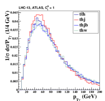
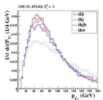
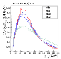
Figure 8: The $P_{T_{\gamma}}$ distributions for the $t\bar{t}h$ and $thX$ processes in the $h\to\gamma\gamma$ channel at LHC-13 taking $C_{t}^{S}=+1\,,-1\,,+1.5\,,-1.5$ from left to right. We use the Delphes ATLAS template for detector simulations.

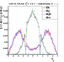
Figure 9: The same as in Fig. 8 but for the $\eta_{j}$ distributions.

Table 12: Selection cuts to disentangle $thX$ from $t\bar{t}h$. The Delphes ATLAS template is used.

LHC-13	ATLAS Analysis Cuts, $h\rightarrow\gamma\gamma$
Basic cuts :	$\Delta R_{ij}>0.4$ with $i,j$ denoting $b$, $j$ and $l$
	$P_{Tb}>25GeV,|\eta_{b}|<2.5$, $P_{Tl}>25GeV,|\eta_{l}|<2.5$, $P_{Tj}>25GeV,|\eta_{j}|<4.7$
$\#$ of $\gamma$ $\&$ Higgs mass window cuts :	$N(\gamma)=2,\ |M_{\gamma\gamma}-m_{h}|<5GeV$
$t\bar{t}h$ search	$|\eta_{j}|<2.5$
$thj$ search	Forward jet-tag : $2.5<|\eta_{j}|<4.7$
$t\rightarrow$ semileptonically $\&$ leptonically :	$N(e$ or $\mu$)=1, $E_{T}^{miss}>20GeV$,
	Invariant Mass cuts for top decay product : $M_{bl}<200GeV$
	$t\bar{t}h$ search : $N(j)\geq 2,N(b)\geq 1$
	$thj$ search : $N(j)\leq 3,N(b)\leq 2$
$t\rightarrow$ hadronically :	$N(e$ or $\mu$)=0, Invariant Mass cuts for top decay product : $M_{bj_{1}j_{2}}<300GeV$
	$t\bar{t}h$ search : $N(j)\geq 6,N(b)\geq 2$
	$thj$ search : $N(j)\leq 5,N(b)\leq 2$

The accumulated $thj$ signal strength $\mu(thj)$ is shown in the left panel of Fig. 10 with $C_{t}^{S}=\pm 1\,,\pm 1.5$. To obtain the signal strength $\mu(thj)$ in the $h\to\gamma\gamma$ decay at LHC-13, we impose the $thj$-specific cuts listed in Table 12. In the right panel of Fig. 10, we show the accumulated $t\bar{t}h$ signal strength $\mu(t\bar{t}h)$ obtained by using the $t\bar{t}h$-specific cuts in the same Table. We observe that $\mu(thj)$ (left) is dominated by $thj$ (green) for the negative values of $C_{t}^{S}$, implying that our $thj$-specific cuts are working very efficiently when the $thj$ production cross section is much enhanced with $R(thj)\>\raisebox{-2.15277pt}{$\stackrel{{\scriptstyle\textstyle>}}{{\sim}}$}\>1$. On the other hand, $\mu(t\bar{t}h)$ (right) is dominated by $t\bar{t}h$ (blue) independently of $C_{t}^{S}$ and we observe that our $t\bar{t}h$-specific cuts are working reasonably well as in the LHC-8 case (the left panel of Fig. 6). We can further draw a few observations from Fig. 10 as follows.

1. When the experiment is targeting at $t\bar{t}h$ production using the $t\bar{t}h$-specific cuts, there are contaminations from the $thX$ processes. For positive $C_{t}^{S}$, the $thX$ contaminations are small. But, for negative $C_{t}^{S}$, they can be as large as the $t\bar{t}h$ signals. For $C_{t}^{S}=-1$, for example, $\mu(t\bar{t}h)\sim 2$ and only half of which comes from $t\bar{t}h$.

2. From the left panel, we can see that the $thX$ processes dominate the signal strength $\mu(thj)$ for negative $C_{t}^{S}$, which means that the $thj$-specific selection cuts we employed indeed can single out the $thj$ process from the $t\bar{t}h$ one.

3. The large values of $\mu(thj)\sim{\cal O}(10)$ when $C_{t}^{S}$ deviates from its SM value $1$ imply that the direct $thj$ searches are also important as complementary channels. Current LHC constraints on the $thj$ searches at $\sqrt{s}=8$ TeV in are still weak thj-8 , so that more data are needed at $\sqrt{s}=13$ TeV in the future to probe the anomalous top-Yukawa coupling through this channel.

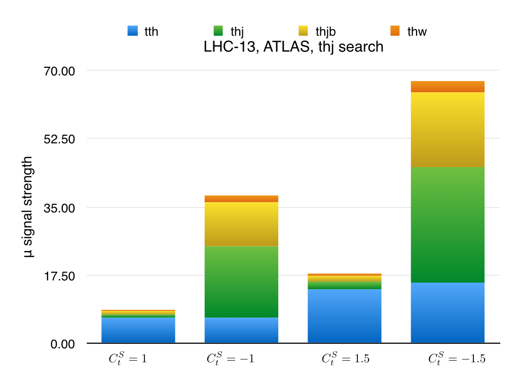
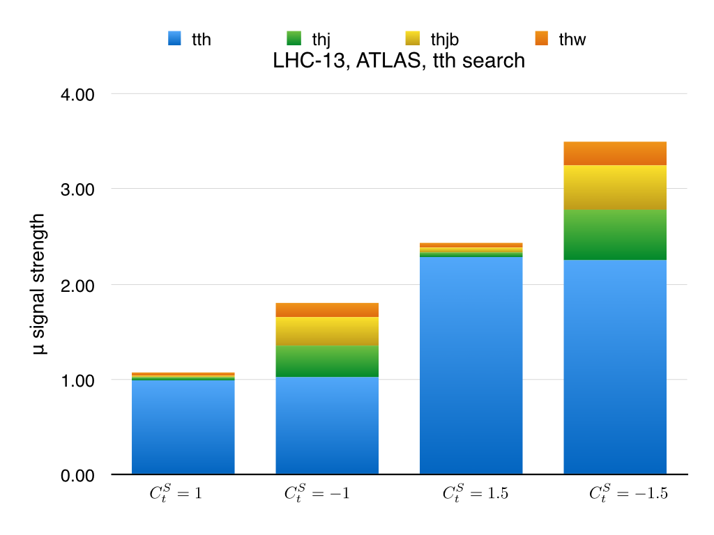
Figure 10: Accumulated signal strengths $\mu(thj)$ (left) and $\mu(t\bar{t}h)$ (right) at LHC-13 obtained by stacking the various $thX$ contributions on the $t\bar{t}h$ one for $C_{t}^{S}=+1\,,-1\,,+1.5\,,-1.5$ from left to right. We use the Delphes ATLAS template for detector simulations.

V Conclusions

Usually, the associated Higgs production with a single top quark dubbed as $thX$ with $X=j,jb,W$ makes only small contributions to the overall experimental signal strength of $\mu(t\bar{t}h)$. In this work, however, we have demonstrated explicitly that the $thX$ processes can significantly increase the experimentally measured signal strength $\mu(t\bar{t}h)$ when the relative sign of the top-Yukawa coupling to the gauge-Higgs coupling is reversed. Furthermore, we have shown explicitly that the $thX$ processes contaminate at quite different levels in various detection modes of $tth$, depending on the value of top-Yukawa coupling, on the cuts used in each experiment, and on the decay mode of the Higgs boson. Such behavior is far more complicated than simply assuming a small constant level of contamination in all channels. The signal strengths can be as large as $2-4$ in the category Leptons for $h\to$ multileptons, $2-4.5$ in the category $\gamma\gamma$ for $h\to\gamma\gamma$, and $2-4$ in the category $b\bar{b}$ for $h\to b\bar{b}$. Assuming the mild excesses observed in $t\bar{t}h$ production at the LHC are real, we note that all go in the right direction to match them.

When more data are collected at $\sqrt{s}=13$ TeV, we can choose more specific cuts to single out the $thX$ processes, which can effectively determine the size and the sign of the top-Yukawa coupling.

We offer the following comments on our findings.

1. The current data on $t\bar{t}h$ production showed mild excesses at some level . Although they may be simply due to statistical fluctuations, in this work, we have taken the liberty of interpreting the mild excesses by exploiting the strong entanglement between $thX$ and $t\bar{t}h$. Our case study would be very useful if the future data support the excesses.

2. When the top-Yukawa coupling is kept at the SM value, i.e. $C_{t}^{S}=1$, the contamination from all the $thX$ processes is small, only about $5-15\%$, and that can be regarded as a sort of small higher-order corrections.

3. However, when the sign of the top-Yukawa coupling is reversed, i.e. $C_{t}^{S}=-1$, the $thX$ contributions are significantly enhanced. And the resulting signal strengths can be as large as $1.4-2.0$ (category Leptons), $1.0-2.5$ (category $\gamma\gamma$), and $1.4-2.0$ (category $b\bar{b}$), explaining the experimental excesses shown in Table 1.

4. When $C_{t}^{S}$ is further negative, say $-1.5$, the resulting signal strength $\mu(t\bar{t}h)$ further increases to $2.7-3.9$ (category Leptons), $2.4-4.5$ (category $\gamma\gamma$), and $2.6-3.8$ (category $b\bar{b}$).

5. In the approach adopted in this work, the dominant $thX$ processes are $thj$ and $thjb$ both of which contain a very forward energetic jet. Also, as shown in Fig. 8, the $thW$ process has a harder $p_{T}$ photon. Therefore, we successfully come up with a set of selection cuts to single out the $thX$ processes from the $t\bar{t}h$ process. It has been shown clearly in the left panel of Fig. 10.

6. One very useful observation in our work is that the contributions from various production processes of $t\bar{t}h$, $thj$, $thjb$, and $thW$ to the accumulated signal strengths strongly depend not only on the Higgs decay channels but also on the experiment (ATLAS or CMS), as can be seen in Figs. 5 – 7.

References

- (1) G. Aad et al. [ATLAS Collaboration], Phys. Lett. B 716, 1 (2012) [arXiv:1207.7214 [hep-ex]].
- (2) S. Chatrchyan et al. [CMS Collaboration], Phys. Lett. B 716, 30 (2012) [arXiv:1207.7235 [hep-ex]].
- (3) See for example, K. Cheung, J. S. Lee and P. -Y. Tseng, JHEP 1305, 134 (2013) [arXiv:1302.3794 [hep-ph]]. K. Cheung, J. S. Lee and P. Y. Tseng, Phys. Rev. D 90, 095009 (2014) doi:10.1103/PhysRevD.90.095009 [arXiv:1407.8236 [hep-ph]].
- (4) P. W. Higgs, Phys. Rev. Lett. 13, 508 (1964); F. Englert and R. Brout, Phys. Rev. Lett. 13, 321 (1964); G. S. Guralnik, C. R. Hagen and T. W. B. Kibble, Phys. Rev. Lett. 13, 585 (1964).
- (5) ATLAS Coll., ”Measurements of the Higgs boson production and decay rates and couplings using pp collision data at sqrt(s)=7 and 8 TeV in the ATLAS experiment”, ATLAS-CONF-2015-007 (March 2015); V. Khachatryan et al. [CMS Collaboration], Eur. Phys. J. C 75, no. 5, 212 (2015) doi:10.1140/epjc/s10052-015-3351-7 [arXiv:1412.8662 [hep-ex]].
- (6) G. Aad et al. [ATLAS Collaboration], JHEP 1510, 150 (2015) doi:10.1007/JHEP10(2015)150 [arXiv:1504.04605 [hep-ex]].
- (7) V. Khachatryan et al. [CMS Collaboration], JHEP 1409, 087 (2014) [JHEP 1410, 106 (2014)] doi:10.1007/JHEP09(2014)087, 10.1007/JHEP10(2014)106 [arXiv:1408.1682 [hep-ex]].
- (8) S. Chatrchyan et al. [CMS Collaboration], JHEP 1401, 163 (2014) [JHEP 1501, 014 (2015)] doi:10.1007/JHEP01(2015)014, 10.1007/JHEP01(2014)163 [arXiv:1311.6736, arXiv:1311.6736 [hep-ex]]. G. Aad et al. [ATLAS Collaboration], JHEP 1406, 035 (2014) doi:10.1007/JHEP06(2014)035 [arXiv:1404.2500 [hep-ex]]. G. Aad et al. [ATLAS Collaboration], Phys. Lett. B 749, 519 (2015) doi:10.1016/j.physletb.2015.07.079 [arXiv:1506.05988 [hep-ex]]. G. Aad et al. [ATLAS Collaboration], JHEP 1511, 172 (2015) doi:10.1007/JHEP11(2015)172 [arXiv:1509.05276 [hep-ex]]. V. Khachatryan et al. [CMS Collaboration], arXiv:1510.01131 [hep-ex].
- (9) B. Bhattacherjee, S. Chakraborty and S. Mukherjee, arXiv:1505.02688 [hep-ph]. P. Huang, A. Ismail, I. Low and C. E. M. Wagner, Phys. Rev. D 92, no. 7, 075035 (2015) doi:10.1103/PhysRevD.92.075035 [arXiv:1507.01601 [hep-ph]]. C. R. Chen, H. C. Cheng and I. Low, arXiv:1511.01452 [hep-ph].
- (10) G. Aad et al. [ATLAS Collaboration], Phys. Lett. B 749, 519 (2015) doi:10.1016/j.physletb.2015.07.079 [arXiv:1506.05988 [hep-ex]].
- (11) J. Chang, K. Cheung, J. S. Lee and C. T. Lu, JHEP 1405, 062 (2014) doi:10.1007/JHEP05(2014)062 [arXiv:1403.2053 [hep-ph]].
- (12) T. M. P. Tait and C.-P. Yuan, Phys. Rev. D 63, 014018 (2000) doi:10.1103/PhysRevD.63.014018 [hep-ph/0007298]. W. J. Stirling and D. J. Summers, Phys. Lett. B 283 (1992) 411. doi:10.1016/0370-2693(92)90040-B A. Ballestrero and E. Maina, Phys. Lett. B 299 (1993) 312. doi:10.1016/0370-2693(93)90265-J G. Bordes and B. van Eijk, Phys. Lett. B 299 (1993) 315. doi:10.1016/0370-2693(93)90266-K F. Maltoni, K. Paul, T. Stelzer and S. Willenbrock, Phys. Rev. D 64 (2001) 094023 doi:10.1103/PhysRevD.64.094023 [hep-ph/0106293]. V. Barger, M. McCaskey and G. Shaughnessy, Phys. Rev. D 81, 034020 (2010) [arXiv:0911.1556 [hep-ph]].
- (13) S. Biswas, E. Gabrielli and B. Mele, JHEP 1301, 088 (2013) [arXiv:1211.0499 [hep-ph]]; S. Biswas, E. Gabrielli, F. Margaroli and B. Mele, JHEP 07, 073 (2013) [arXiv:1304.1822 [hep-ph]]. M. Farina, C. Grojean, F. Maltoni, E. Salvioni and A. Thamm, JHEP 1305, 022 (2013) [arXiv:1211.3736 [hep-ph]]. P. Agrawal, S. Mitra and A. Shivaji, arXiv:1211.4362 [hep-ph]. J. Ellis, D. S. Hwang, K. Sakurai and M. Takeuchi, arXiv:1312.5736 [hep-ph]. C. Englert and E. Re, arXiv:1402.0445 [hep-ph]. A. Kobakhidze, L. Wu and J. Yue, JHEP 1410, 100 (2014) doi:10.1007/JHEP10(2014)100 [arXiv:1406.1961 [hep-ph]]. F. Demartin, F. Maltoni, K. Mawatari, B. Page and M. Zaro, Eur. Phys. J. C 74 (2014) no.9, 3065 doi:10.1140/epjc/s10052-014-3065-2 [arXiv:1407.5089 [hep-ph]]. S. Khatibi and M. Mohammadi Najafabadi, Phys. Rev. D 90 (2014) no.7, 074014 doi:10.1103/PhysRevD.90.074014 [arXiv:1409.6553 [hep-ph]]. J. Yue, Phys. Lett. B 744, 131 (2015) doi:10.1016/j.physletb.2015.03.044 [arXiv:1410.2701 [hep-ph]]. F. Demartin, F. Maltoni, K. Mawatari and M. Zaro, Eur. Phys. J. C 75, no. 6, 267 (2015) doi:10.1140/epjc/s10052-015-3475-9 [arXiv:1504.00611 [hep-ph]]. M. R. Buckley and D. Goncalves, Phys. Rev. Lett. 116 (2016) no.9, 091801 doi:10.1103/PhysRevLett.116.091801 [arXiv:1507.07926 [hep-ph]]. D. Goncalves, F. Krauss, S. Kuttimalai and P. Maierhöfer, Phys. Rev. D 92 (2015) no.7, 073006 doi:10.1103/PhysRevD.92.073006 [arXiv:1509.01597 [hep-ph]]. F. Demartin, B. Maier, F. Maltoni, K. Mawatari and M. Zaro, arXiv:1607.05862 [hep-ph]. S. D. Rindani, P. Sharma and A. Shivaji, arXiv:1605.03806 [hep-ph].
- (14) F. Maltoni, D. L. Rainwater and S. Willenbrock, Phys. Rev. D 66 (2002) 034022 doi:10.1103/PhysRevD.66.034022 [hep-ph/0202205]; A. Belyaev and L. Reina, JHEP 0208 (2002) 041 doi:10.1088/1126-6708/2002/08/041 [hep-ph/0205270].
- (15) J. S. Lee, A. Pilaftsis, M. S. Carena, S. Y. Choi, M. Drees, J. R. Ellis and C. E. M. Wagner, Comput. Phys. Commun. 156 (2004) 283 [hep-ph/0307377].
- (16) G. Aad et al. [ATLAS Collaboration], Phys. Lett. B 740, 222 (2015) doi:10.1016/j.physletb.2014.11.049 [arXiv:1409.3122 [hep-ex]].
- (17) G. Aad et al. [ATLAS Collaboration], Eur. Phys. J. C 75, no. 7, 349 (2015) doi:10.1140/epjc/s10052-015-3543-1 [arXiv:1503.05066 [hep-ex]].
- (18) J. Alwall et al., JHEP 1407, 079 (2014) doi:10.1007/JHEP07(2014)079 [arXiv:1405.0301 [hep-ph]].
- (19) T. Sjostrand, S. Mrenna and P. Z. Skands, Comput. Phys. Commun. 178, 852 (2008) doi:10.1016/j.cpc.2008.01.036 [arXiv:0710.3820 [hep-ph]].
- (20) J. de Favereau et al. [DELPHES 3 Collaboration], JHEP 1402, 057 (2014) [arXiv:1307.6346 [hep-ex]].
- (21) V. Khachatryan et al. [CMS Collaboration], Phys. Lett. B 749, 337 (2015) doi:10.1016/j.physletb.2015.07.053 [arXiv:1502.07400 [hep-ex]].
- (22) A. Djouadi, J. Kalinowski, M. Spira [arXiv:9704448 [hep-ph]].
- (23) The ATLAS collaboration [ATLAS Collaboration], “Search for the Associated Production of a Higgs Boson and a Top Quark Pair in Multilepton Final States with the ATLAS Detector,” ATLAS-CONF-2016-058; The ATLAS collaboration [ATLAS Collaboration], “Measurement of fiducial, differential and production cross sections in the decay channel with 13.3 fb-1 of 13 TeV proton-proton collision data with the ATLAS detector”, ATLAS-CONF-2016-067; The ATLAS collaboration [ATLAS Collaboration], “Search for the Standard Model Higgs boson produced in association with top quarks and decaying into a bb pair in pp collisions at = 13 TeV with the ATLAS detector,” ATLAS-CONF-2016-080; The ATLAS collaboration [ATLAS Collaboration], “Combination of the searches for Higgs boson production in association with top quarks in the , multilepton, and decay channels at =13 TeV with the ATLAS Detector,” ATLAS-CONF-2016-068.
- (24) CMS Collaboration [CMS Collaboration], “Search for associated production of Higgs bosons and top quarks in multilepton final states at ,” CMS-PAS-HIG-16-022; CMS Collaboration [CMS Collaboration], “Updated measurements of Higgs boson production in the diphoton decay channel at TeV in pp collisions at CMS”, CMS-PAS-HIG-16-020. CMS Collaboration [CMS Collaboration], “Search for production in the decay channel with 2016 pp collision data at ,” CMS-PAS-HIG-16-038.
- (25) CMS Collaboration [CMS Collaboration], “Search for H to bbbar in association with single top quarks as a test of Higgs couplings,” CMS-PAS-HIG-14-015; C. Boser [ATLAS and CMS Collaborations], “Experimental searches for tHq,” arXiv:1411.2988 [hep-ex]; A. Popov [CMS Collaboration], “Identification of signal events in a search for produced in association with single top quarks,” arXiv:1411.7170 [hep-ex]; V. Khachatryan et al. [CMS Collaboration], “Search for the associated production of a Higgs boson with a single top quark in proton-proton collisions at TeV,” JHEP 1606, 177 (2016) doi:10.1007/JHEP06(2016)177 [arXiv:1509.08159 [hep-ex]]; K. Bloom, “Search for associated production of a Higgs boson with a single top quark,” arXiv:1510.00894 [hep-ex]; CMS Collaboration [CMS Collaboration], “Search for Associated Production of a Single Top Quark and a Higgs Boson in Leptonic Channels,” CMS-PAS-HIG-14-026; L. Caminada [CMS Collaboration], “Higgs boson production in association with top quarks in CMS,” Nucl. Part. Phys. Proc. 270-272, 217 (2016). doi:10.1016/j.nuclphysbps.2016.02.043