Estimating Causal Peer Influence in Homophilous Social Networks by Inferring Latent Locations

Abstract

Social influence cannot be identified from purely observational data on social networks, because such influence is generically confounded with latent homophily, i.e., with a node’s network partners being informative about the node’s attributes and therefore its behavior. If the network grows according to either a latent community (stochastic block) model, or a continuous latent space model, then latent homophilous attributes can be consistently estimated from the global pattern of social ties. We show that, for common versions of those two network models, these estimates are so informative that controlling for estimated attributes allows for asymptotically unbiased and consistent estimation of social-influence effects in linear models. In particular, the bias shrinks at a rate which directly reflects how much information the network provides about the latent attributes. These are the first results on the consistent non-experimental estimation of social-influence effects in the presence of latent homophily, and we discuss the prospects for generalizing them.

1 Introduction: Separating Homophily from Social Influence

It is an ancient observation that people are influenced by others (nearby) in their social network—that is, the behavior of one node in a social network adapts or responds to that of neighboring nodes. Such social influence is not just a curiosity, but of deep theoretical and empirical importance across the social sciences. It is also of great importance to various kinds of social engineering, e.g., marketing (especially, but not only, “viral” marketing), public health (over-coming “peer pressure” to engage in risky behaviors, or using it to spread healthy ones), education (“peer effects” on learning), politics (“peer effects” on voting), etc. Conversely, it is an equally ancient observation that people are not randomly assigned their social-network neighbors. Rather, they select them, and tend to select as neighbors those who are already similar to themselves. (This is not necessarily because they prefer those who are similar; all more-desirable potential partners might have already been claimed or otherwise excluded (Martin, 2009).) This homophily means that network neighbors are informative about latent qualities a node possesses, providing an alternative route by which a node’s behavior can be predicted from their neighbors. Efforts to separate homophily from influence have a long history in studies of networks (Leenders, 1995). Motivated by the controversy over Christakis and Fowler (2007), Shalizi and Thomas (2011) showed that unless all of the nodal attributes which are relevant to both social-tie formation and the behavior of interest are observed, then social-influence effects are generally unidentified. The essence of this result is that a social network is a machine for creating selection bias.

Shalizi and Thomas (2011, §4.3) did hint at a possible approach for identification of social influence, even in an homophilous network. When a network forms by homophily, a node is likely to be similar to its neighbors. Following this logic, these neighbors are likely to be similar to their neighbors and therefore the original node. In the simplest situations, where there are only a limited number of node types, this means that a homophilous network should tend to exhibit clusters with a high within-cluster tie density and a low density of ties across clusters. Breaking the network into such clusters might, then, provide an observable proxy for the latent homophilous attributes. The same idea would work, mutatis mutandis, when those attributes are continuous. Shalizi and Thomas (2011) therefore conjectured that, under certain assumptions on the network-growth process (which they did not specify), unconfounded causal inferences could be obtained by controlling for estimated locations in a latent space. Subsequently, Davin et al. (2014) and Worrall (2014) showed that, in limited simulations, such controls can indeed reduce the bias in estimates of social influence, at least when the network grows according to certain, particularly well-behaved, models.

In this paper, we complement these simulation studies by establishing sufficient conditions under which controlling for estimated latent locations leads to asymptotically unbiased and consistent estimates of social-influence effects. Additionally, we show that for a particular class of network models, the remaining finite-sample bias shrinks exponentially in the size of the network, while this bias shrinks polynomially for a more general class of network models. To the best of our knowledge, our results provide the first theoretical guarantees of consistent estimation of social-influence effects from non-experimental data, in the face of latent homophily. Additionally, we provide our own simulations to support and explore our theoretical results.

Section 2 lays out the basics of our setting, starting with assumptions about the processes of network formation and social influence (and the links between them), and rehearsing relevant results from the prior literature on latent community models (§2.2) and continuous latent space models (§2.3). Section 3 presents our main results about the asymptotic estimation of social influence in the presence of latent homophily (proofs are deferred to §6). Section 4 provides a set of simulations that confirm our theoretical results and explore settings that diverge from ours. Section 5 discusses the strengths and limits of our results in the context of the related literature.

2 Setting and Assumptions

The graphical causal model capturing social influence in our setting is shown in Figure 1. More specifically, we are interested in the patterns of a certain behavior or outcome over time, across a social network of $n$ nodes. The behavior of node $i\in\{1,\ldots,n\}$ at time $t\in\{1,\ldots,T\}$ is observed and represented by random variable $Y_{i,t}\in\mathbb{R}$, for some given time-horizon $T$. Social network ties (or links) are also observed and represented through an $n\times n$ adjacency matrix $A$, with $A_{ij}=1$ if $i$ receives a tie from $j$, and $A_{ij}=0$ otherwise. In many contexts these ties are undirected, so $A_{ij}=A_{ji}$, but generally our results do not require this. (In the latent community setting [§2.2], the procedure considered by Gao et al. (2017) assumes an undirected network, and therefore the results of ours which rely on that procedure also make this assumption.) As this notation suggests, we assume that the network of social ties does not change, at least over the time-scale of the observations.

In addition to the observed behaviors and ties of node $i$, we assume there exist a $d$-dimensional latent vector $C_{i}$ which controls its location in the network; we define $C$ as the array $[C_{1},C_{2},\ldots,C_{n}]$. Furthermore, we assume that $\mathrm{Pr}\left(A_{ij}=1|C\right)=w(C_{i},C_{j})$ for some measurable function $w$, and that the random variables $A_{ij}$ and $A_{lm}$ are conditionally independent given $C$, $\forall~{}i,j\neq l,m$. The time-invariant vector $X_{i}$ represents the set of all other (i.e., network irrelevant) attributes for node $i$, which effect $Y_{i,t}$ but not $A_{ij}$.

Figure 1: The graphical causal model for our setting. Boxes indicate observables, and circles latent variables; solid lines indicate causal relations between observables (either autoregressive or peer-influence), while dotted lines indicate the influence of latent homophilous variables, and dashed lines indicate the influence of other covariates. For simplicity, we omit $Y(j,t+1)$ and $Y(l,t+1)$, as well as their associated arrows.

The linear structural-equation model that explains the behavior of node $i$ at time $t$ is thus

$$Y_{i,t+1}=\alpha_{0}+\alpha_{1}Y_{i,t}+\beta\frac{\sum_{j}{\left(Y_{j,t}A_{ij}\right)}}{\sum_{j}{A_{ij}}}+\gamma_{1}^{T}C_{i}+\gamma_{2}^{T}X_{i}+\epsilon_{i,t+1}~{},$$ (1)

where $\gamma_{1}$ and $\gamma_{2}$ serve as appropriately-sized vectors of coefficients. Under the assumptions of linearly-independent regressors and strict exogeneity—i.e., $\mathbb{E}\left[\epsilon_{i,t+1}|Y_{i,t},A_{ij},C_{i},X_{i}\right]=0~{}\forall i,j,t$—our goal is to identify, and estimate, $\beta$, the coefficient for social influence. Given that we neither observe $X_{i}$ nor $C_{i}$, we cannot estimate the regression coefficients in a model of the form presented in (1). However, we can estimate the coefficients of the following model:

$$Y_{i,t+1}=\alpha_{0}+\alpha_{1}Y_{i,t}+\beta\frac{\sum_{j}{\left(Y_{j,t}A_{ij}\right)}}{\sum_{j}{A_{ij}}}+\gamma_{0}^{T}\hat{C}_{i}+\eta_{i,t+1}~{},$$ (2)

where $\hat{C}_{i}$ is an estimated or discovered location for node $i$ and the noise term $\eta_{i,t+1}$ can be defined as

$$\eta_{i,t+1}=\epsilon_{i,t+1}+\gamma_{2}^{T}X_{i}+\left(\gamma_{1}^{T}C_{i}-\gamma_{0}^{T}\hat{C}_{i}\right)~{}.$$

Our general setting is therefore defined by an additional assumption:

$$X_{i}\rotatebox{90.0}{$\models$}Y_{j,t}|\hat{C}_{i}.$$ (3)

The assumptions of independence must be justified on substantive grounds, in the specific context of the study where social influence is being estimated.

2.1 Discussion on the General Setting

We find it beneficial to provide intuition on how various facets of our setting enable the identification of social-influence effects. We begin by recognizing that the relatively permanent attributes of node $i$ can be divided in two cross-cutting ways. On the one hand, some attributes are (in a given study) observable or manifest, and others are latent. On the other hand, a given attribute could be a cause of the behavior of interest $Y_{i,t}$, or a cause of network ties ($A_{ij}$), or of both. (Attributes which are irrelevant to both behavior and network ties are ignored here as they have no bearing on our ultimate goal).

One of the key assumptions embedded in our tie formation process (i.e., $\mathrm{Pr}\left(A_{ij}=1|C\right)=w(C_{i},C_{j})$) is that all of the network-relevant attributes of node $i$ can be represented by a single vector-valued latent variable $C_{i}$, whether or not they are also relevant to the behavior of interest. There may be attributes that are incorporated into $C_{i}$ which are relevant only to network ties, not behavior, and independent of the other attributes; these are of no concern to us, and can be regarded as part of the noise in the tie-formation process. Network models that satisfy this assumption—i.e., that all ties are conditionally independent of each other given the latent variables for each node—are sometimes called “graphons” or “$w$-random graphs” and are clearly exchangeable (permutation-invariant) over nodes. Conversely, the Aldous-Hoover theorem (Kallenberg, 2005, ch. 7) shows that this condition is, in fact, the generic form of exchangeable random networks. Our subsequent assumption, speaking roughly, is that by observing the whole network $A_{ij}$ (which inherently includes the information it contains with respect to the latent array $C$), $Y_{i,t}$ provides no additional information (in the limit) for node $i$’s latent location $C_{i}$.

We also recognize that as a result of the assumptions of linear-dependence and strict exogeneity in (1), if all the variables relevant to tie-formation and node behavior are observed, the ordinary least squares (OLS) estimator provides an unbiased estimate ($\hat{\beta}_{OLS}$) of $\beta$. However, since $C_{i}$ and $X_{i}$ are both unobserved, and therefore their effects are contained in the $\eta_{i,t+1}$ of (2), $\hat{\beta}_{OLS}$ will generally contain omitted variable bias if either of these latent variables are correlated with $Y_{j,t}$, conditional on the observed regressors. Intuitively, the latent nature of $X_{i}$ will not produce bias because (3) implies that given estimated locations, nothing can be learned about a node’s unobserved, network-irrelevant attributes by observing a neighbor’s behavior (or vice-versa). Mathematically, this means that the contribution of $\gamma_{2}^{T}X_{i}$ to $\eta_{i,t+1}$ is uncorrelated with $Y_{j,t}$, given the estimated locations, and therefore this term does not bias the estimates of $\beta$; instead it just increases the variance of the noise term. It is also not necessary that $E[\eta_{i,t+1}]=0$; if it has a non-zero value, it would then be incorporated into the estimate of the intercept ($\alpha_{0}$), and therefore not induce bias in $\beta$. We have therefore to only consider the other contribution to $\eta_{i,t+1}$, $(\gamma_{1}C_{i}-\gamma_{0}\hat{C}_{i})$, and whether it is correlated with $Y_{j,t}$ given $\hat{C}_{i}$ and $Y_{i,t}$.

$\lVert C_{i}-\hat{C}_{i}\rVert$ is the error in estimating the true location, which manifests as measurement error in OLS estimation of $\beta$ in (2). Given that $Y_{j,t}$ is a causal descendant of $C_{j}$, and $C_{j}$ is positively correlated with $C_{i}$ if $A_{ij}=1$ (from homophily), this measurement error induces bias in the estimate of $\beta$. Intuitively (and formally shown in Lemma 1 below) if $\hat{C}=C$ (i.e., there is no measurement error) the OLS estimate of $\beta$ in (2) will be unbiased and consistent; although, this estimate will likely have a larger variance than would the OLS estimate of $\beta$ from (1), given that the former estimate does not control for $X_{i}$. It should further be plausible (and is formally shown in §3 below) that if $\hat{C}$ is a “good enough” estimate of $C$—i.e., one which is consistent and converges sufficiently rapidly—the covariance between $\eta_{i,t+1}$ and $Y_{j,t}$ shrinks fast enough that the OLS estimate from (2) will still yield asymptotically unbiased and consistent estimates of $\beta$. Essentially, the OLS estimator for $\beta$ in (2) trades-off the bias (experienced by the OLS estimator for $\beta$ in (1)) from omitting the latent location variable $C_{i}$, with the bias from measuring (estimating) the location imprecisely with $\hat{C}_{i}$. However, the ability to obtain a “good enough” estimate of $C$ will make this trade-off worthwhile; if the measurement error converges to zero, then the bias it induces should also converge to zero, while the omitted variable bias persists.

There does not (yet) exist results providing such “good enough” estimates of latent node locations $\hat{C}$ for arbitrary graphons. For this reason, our results specialize to two settings, where the latent node locations $C$ and the link-probability function $w$ take particularly tractable forms: latent community (stochastic block) models and the more general (continuous) latent space models. Both model types have been extensively explored in the literature. It is by building on results for these models that we can find regimes where the social-influence coefficients can be estimated consistently. It is, however, worth noting that for any graphon model where “good enough” estimates of latent node locations $\hat{C}$ exist, an analog to our results for latent space models (Theorem 2) can be built.

2.2 The Latent Communities Setting

In our first setting, we presume that nodes split into a finite number of discrete types or classes ($k$), which in this context are called blocks, modules or communities. More precisely, there exists a function $\sigma\colon\{1,\dots,n\}\mapsto\{1,\dots,k\}$ assigning nodes to communities. We specifically assume that the network is generated by a stochastic block model, which is to say that there are $k$ communities, that $\sigma(i)\overset{iid}{\sim}\rho$, for some fixed (but unknown) multinomial distribution $\rho$, and that $w$ is given by a $k\times k$ affinity matrix, so that

$$\mathrm{Pr}\left(A_{ij}=1|\sigma(i)=a,\sigma(j)=b\right)=w_{ab}~{}.$$

We may translate between $\sigma$ (a sequence of categorical variables) and our earlier $C$ (an $n\times d$ matrix of node locations) by the usual device of introducing indicator or “dummy” variables for $k-1$ of the communities, so that $C_{i}$ is a $k-1$ binary vector (i.e., $d=k-1$) which is a function of $\sigma(i)$ and vice versa. Each possible value of $C_{i}$ is either the origin, or a corner of the simplex; this basic observation will be important below.

The objective of community detection or community discovery is to provide an accurate estimate $\hat{\sigma}$ or $\hat{C}$ from the observed adjacency matrix $A$, i.e., to say which community each node comes from, subject to a permutation of the label set. (“Accuracy” here is often measured as the proportion of mis-classification.) Since the problem was posed by Girvan and Newman (2002) a vast literature has emerged on the topic, spanning many fields, including physics, computer science, and statistics; see Fortunato (2010) for a review. However, we may summarize the most relevant findings as follows.

1. For networks which are generated from latent community models, under very mild regularity conditions, it is possible to recover the communities consistently, i.e., as $n\rightarrow\infty$, $\mathrm{Pr}\left(\hat{C}\neq C\right)\rightarrow 0$ (Bickel and Chen, 2009; Zhao et al., 2012). That is, with probability tending to one, all of the community assignments are correct, up to a global permutation of the labels between $C$ and $\hat{C}$.

2. Such consistent community discovery can be achieved by algorithms whose running time is polynomial in $n$.

3. The minimax rate of convergence is in fact exponential in $n$ (and can be achieved by the algorithms mentioned below).

These points, particularly the last, will be important in our argument below, and so we now elaborate on them.

Recently, Zhang and Zhou (2016) proved that under very mild regularity conditions the minimax rate of convergence for undirected networks generated from latent community models is in fact exponential in $n$. Furthermore, Gao et al. (2017) exploits techniques provided by Zhang and Zhou (2016) to propose an algorithm polynomial in $n$ that achieves this minimax rate, under slightly modified but equally mild regularity conditions. More precisely, Gao et al. (2017) considers a general undirected stochastic block model, parametrized by $n$, the number of nodes; $k$, the number of communities; $a$ and $\alpha\geq 1$, where $\frac{a}{n}=\min_{i}{w(i,i)}\leq\max_{i}{w(i,i)}\leq\frac{\alpha a}{n}$, ensuring that within-community edges are “sufficiently” dense; $b$, where $\frac{b\alpha}{n}\leq\frac{1}{k(k-1)}\sum_{i\neq j}{w(i,j)}\leq\max_{i\neq j}{w(i,j)}\frac{b}{n}$, with $0<\frac{b}{n}<\frac{a}{n}<1$, ensuring that between-community edges are “sufficiently” sparse; and $\beta\geq 1$, where the number of nodes in community $k$, $n_{k}\in\left[\frac{n}{\beta k},\frac{\beta n}{k}\right]$, ensuring that community sizes are “sufficiently” comparable. Zhang and Zhou (2016) and Gao et al. (2017) diverge slightly as the former only requires $\max_{i\neq j}{w(i,j)}\leq\frac{b}{n}$ and $\frac{a}{n}\leq\min_{i}{w(i,i)}$. Additionally, the latter slightly restricts the parameter space by requiring the $k^{th}$ singular value of the affinity matrix $w$ to be greater than some parameter $\lambda$. The general context of the theory described in Zhang and Zhou (2016); Gao et al. (2017) is defined for absolute constant $\beta\geq 1$ and also in Gao et al. (2017) for absolute constant $\alpha\geq 1$, while $k$, $a$, $b$, and $\lambda$ are functions of $n$ and therefore vary as $n$ grows. However, in our context, the network does not change (over the time-scale of interest); therefore, we only consider latent communities where $k$, $\frac{a}{n}$, $\frac{b}{n}$, and $\lambda$ are also absolute constants. We shall refer to this whole set of restrictions on the latent community model as “the GMZZ conditions”.

For a latent community model satisfying the GMZZ conditions, the minimax rate of convergence for the expected proportion of errors is

$$\exp{\left(-(1+o(1))\frac{nI}{2}\right)}, \quad k=2$$ (4)

$$\exp{\left(-(1+o(1))\frac{nI}{\beta k}\right)}, \quad k\geq 3,$$ (5)

where $I$ is the Rényi (1961) divergence of order $\frac{1}{2}$ between two Bernoulli distributions with success probabilities $\left(\frac{a}{n}\right)$ and $\left(\frac{b}{n}\right)$: $D_{\frac{1}{2}}\left(\text{Ber}\left(\frac{a}{n}\right)\|\text{Ber}\left(\frac{b}{n}\right)\right)$. Recall that $\beta$ in addition to $k$, $\frac{a}{n}$, $\frac{b}{n}$ are, in our context, constant in $n$; therefore, (4) and (5) both reduce to $\exp{\left(-O(n)\right)}$. The algorithm of Gao et al. (2017) achieves this rate at a computational cost polynomial in $n$. More specifically, the time complexity of the algorithm is (by our calculations) at most $O(n^{3})$, but we do not know whether this is tight. It would be valuable (but beyond the scope of this work) to know whether this rate is also a lower bound on the computational cost of obtaining minimax error rates, and if the complexity could be reduced in practice for very large graphs via parallelization.

We close this section by introducing a bit of notation (which will simplify some later statements) and making a claim (which will be supported later). We will write $\delta(n)$ for the error probability, i.e., the probability that $\hat{C}_{i}\neq C_{i}$ for at least one $i\in 1:n$. The claim is that even though the results of Zhang and Zhou (2016) and Gao et al. (2017) concern the proportion of mis-classified nodes, they actually constrain the probability of making any mis-classifications at all, and imply $\delta(n)=e^{-O(n)}$ (Lemma 3).

2.3 The Continuous Latent Space Setting

The second setting we consider is that of continuous latent space models. In this setting, the latent variable on each node, $C_{i}$, is a point in a continuous metric space (often but not always $\mathbb{R}^{d}$ with the Euclidean metric), and $w(C_{i},C_{j})$ is a decreasing function of the distance between $C_{i}$ and $C_{j}$, e.g., a logistic function of the distance. This link-probability function is often taken to be known a priori. The latent locations $C_{i}\overset{iid}{\sim}F$, where $F$ is a fixed but unknown distribution, or, more rarely, a point process. Different distributions over networks thus correspond to different distributions over the continuous latent space, and vice versa.

Parametric versions of this model have been extensively developed since Hoff et al. (2002), especially in Bayesian contexts. Less attention has been paid to the consistent estimation of the latent locations in such models, than to the estimation of community assignments in latent community models. Recent results by Asta (2015, ch. 3), however, show that when $w$ is a smooth function of the metric whose logit transformation is bounded, the maximum likelihood estimate $\hat{C}$ converges to $C$. Moreover, the probability of an error of size $\epsilon$ or larger is $O(\exp{\left(-\kappa\epsilon n^{2}\right)})$, where the constant $\kappa$ depends on the purely geometric properties of the space (see §3.2 below). This result holds across distributions of the $C_{i}$, but may not be the best possible rate.

3 Control of Confounding

Given the (assumed) true structural equation in (1), our ultimate goal is to provide both an estimator of $\beta$, and the corresponding sufficient conditions under which that estimator will have desirable statistical properties. Recall that these properties of the estimator are evaluated in the presence of estimated or discovered node locations $\hat{C}$, rather than the true locations $C$. Going forward, therefore, unless otherwise noted, our estimator of interest is OLS for $\beta$ in (2). Finally, all proofs of the results stated below are provided in §6.

We begin by establishing this estimator’s properties in a baseline case: when the estimates of node locations are perfect, $\mathrm{Pr}\left(C\neq\hat{C}\right)=0$.

Lemma 1.

Under the assumptions from Section 2, if $\mathrm{Pr}\left(C\neq\hat{C}\right)=0$, then the ordinary least squares estimate of $\beta$ in (2) is unbiased and consistent.

Given that we establish that OLS estimator will exhibit unbiasedness and consistency, when node locations can be perfectly inferred, let us now consider its properties when the node location are inferred with error. The covariance of interest is that between $\frac{\sum_{j}{\left(Y_{j,t}A_{ij}\right)}}{\sum_{j}{A_{ij}}}$ and the contribution to the error—i.e., $\eta_{i,t+1}$ in (2)—arising from using the estimated rather than the real communities. We have seen (§2.1), that in our setting, under assumption (3), this term is just $\gamma_{1}^{T}C_{i}-\gamma_{0}^{T}\hat{C}_{i}$. Moreover, we will only need to consider that covariance conditional on $\hat{C}_{i}$ and $\hat{C}_{j}$, and the other regressor in (2), i.e., $Y_{i,t}$.

Lemma 2.

Suppose that the assumptions from Section 2 hold. Then

$$\mathrm{Cov}\left[\frac{\sum_{j}{\left(Y_{j,t}A_{ij}\right)}}{\sum_{j}{A_{ij}}},(\gamma_{1}^{T}C_{i}-\gamma_{0}^{T}\hat{C}_{i})\middle|A,Y_{i,t}\right]$$ (6)

$$~{}=\frac{\sum_{j}{A_{ij}\gamma_{1}^{T}\left(\mathrm{Cov}\left[C_{i},C_{j}\middle|A\right]+\xi_{ij}\mathrm{Var}\left[C_{i}|A\right]+\sum_{l\neq i,j}{\zeta_{ijl}\mathrm{Cov}\left[C_{i},C_{l}|A\right]}\right)\gamma_{1}}}{\sum_{j}{A_{ij}}},$$

where by $\mathrm{Cov}\left[C_{i},C_{j}\right]$ we mean the $d\times d$ matrix of coordinate-wise covariances, and similarly for $\mathrm{Var}\left[C_{i}\right]$, and the $\xi$s and $\zeta$s are constants calculable in terms of the model coefficients and the adjacency matrix (and are made explicit in the proof of the lemma).

Lemma (2) establishes an important relationship between the bias experienced by the OLS estimator and the degree of homophily in the network. Recall that we observe a network (represented by $A$) whose ties are formed under homophily, based on (unobserved) node locations. Furthermore, it is precisely the fact that this network is observed (and conditioned on) that opens the confounding backdoor pathway in the causal graph (Figure 1). For clarity, the network is conditioned on because it enables the true structural equation (1) to select if the behavior of node $i$ is regressed on the behaviors of nodes $j$. Moreover, when homophily has a large impact on tie formation, the value $\mathrm{Cov}\left[C_{i},C_{j}\right]$ will be large, as node $i$ will have more connections from closer nodes $j$ (i.e., roughly, $C_{i}\approx C_{j}$). We then recognize that although observing the network $A$ (and failing to observe the latent locations $C$) opens the homophilous confounding pathway, the network also manifests this homophily in the ties that are formed, which can be used to form estimates of the latent locations $\hat{C}$. Further, conditioning on $A$ implies conditioning on $\hat{C}_{i}$ and $\hat{C}_{j}$, as they are deterministic (albeit complicated) functions of $A$. From Lemma (2) we then see that the bias in our estimate $\hat{\beta}_{OLS}$ is proportional to the amount of covariance between the true latent locations of nodes that share a tie, beyond that which is accounted for by their location estimates. Therefore, when this conditional covariance is zero, $\hat{\beta}_{OLS}$ is unbiased and consistent.

There are two individually sufficient (but not necessary) conditions for (6) to be zero:

1. $C_{i}\rotatebox{90.0}{$\models$}C_{j}|\hat{C_{i}},\hat{C_{j}}$, i.e., $C_{i}$ and $C_{j}$ are independent given their estimates,

2. $C_{i}=\hat{C_{i}}$ and $C_{j}=\hat{C_{j}}$, i.e., $C_{i}$ and $C_{j}$ are equal to their estimates.

The second condition will generally not be true at any finite $n$. The first condition is also very strong; it implies that $\hat{C}$ is (roughly speaking) a sufficient statistic for $C$. This sufficiency property implies that even in learning $C_{i}$ (the true location of node $i$) we obtain no additional information about $C_{j}$ (the location of any other node $j$) not already captured in $\hat{C}$. We are not aware of any estimates of latent node locations in network models which have such a sufficiency property, and we strongly suspect this is because they generally are not sufficient. (To get a sense of what would be entailed, suppose that $A_{ij}=1$, and we knew we were dealing with a homophilous latent community model. Then $\hat{C}$ would have to be so informative that even if an Oracle told us $C_{i}$, our posterior distribution over $C_{j}$ would be unchanged.) We may, however, make further progress in the two specific settings of latent communities and of continuous latent spaces.

3.1 Control of Confounding with Latent Communities

Let us first consider the setting where the network formation is that of a homophilous latent community process, which follows the conditions laid out in §2.2. In such a setting, we can make additional statements with respect to the $\mathrm{Cov}\left[C_{i},C_{j}\middle|\hat{C}_{i},\hat{C}_{j}\right]$, and subsequently the bias experienced by the OLS estimator. More specifically, these statements are made assuming a deterministic and minimax algorithm—one that achieves the minimax rate of convergence for the expected proportion of node location errors —is utilized to estimate $\hat{C}$ as in Gao et al. (2017).

Lemma 3.

Suppose that the assumptions from Section 2 hold, the network forms according to a latent community model, satisfying the GMZZ conditions, and $\hat{C}$ is estimated using a minimax algorithm. Then

$$\mathrm{Pr}\left(\sum_{i}^{n}{\mathbbm{1}\{\hat{C}_{i}\neq C_{i}\}}\geq 1\right)\leq e^{-O(n)}.$$

We therefore have that the probability of making any error in the estimation of latent node locations converges (exponentially) to zero in $n$. This result from Lemma 3 will play a critical role in proving the next result:

Lemma 4.

Suppose that the assumptions from Section 2 hold, the network forms according to a latent community model, and $\hat{C}$ is estimated by a deterministic algorithm with error rate $\delta(n)$. Then

$$\mathrm{Cov}\left[C_{i},C_{j}\middle|A\right]=O(\delta(n)).$$

If, in addition, the latent community model satisfies the GMZZ equations, and $\hat{C}$ is estimated using a minimax algorithm, then

$$\mathrm{Cov}\left[C_{i},C_{j}\middle|A\right]=O\left(e^{-O(n)}\right).$$

The ability to not only show the convergence of $\mathrm{Cov}\left[C_{i},C_{j}\middle|A\right]$, but also its rate of decay for finite-$n$ leads to a number of important conclusions.

Theorem 1.

Suppose that the assumptions from Section 2 hold, the network forms according to a latent community model, and $\hat{C}$ is estimated with error rate $\delta(n)$. Then the ordinary least squares estimate for $\beta$ in (2) is asymptotically unbiased and consistent, and the pre-asymptotic bias is $O(\delta(n))$. If, in addition, the latent community model satisfies the GMZZ conditions and $\hat{C}$ is estimated using a deterministic and minimax algorithm, then the pre-asymptotic bias is exponentially small in $n$.

We suspect that it is also possible to provide a precise expression of a deterministic finite-$n$ bound on the bias—likely as the solution to an optimization problem involving (unknown) parameters of the structural equation (1)—but leave this as a useful topic for future investigation.

Note: We have stated Lemma 4 and Theorem 1 (and the subsidiary Lemma 5) in two parts to clarify that most of their logic will apply whenever some deterministic algorithm is capable of community discovery with a vanishing error rate $\delta(n)$. The GMZZ conditions are invoked as regularity conditions under which $\delta(n)$ can be made exponentially small at only a polynomial computational cost. If the GMZZ conditions are implausible for a particular application, but some other algorithm can, in that situation, deliver $\delta(n)\rightarrow 0$, then it can be used instead within the scope of our analysis.

3.2 Control of Confounding with Continuous Latent Space

We now turn our attention to setting where the network follows a homophilous continuous latent space model. Recall that our treatment of the latent community setting relies on the fact that $\mathrm{Pr}\left(\hat{C}\neq C\right)\rightarrow 0$, i.e., with probability tending to one the estimated communities match the actual communities exactly. Importantly, this is not known to happen for continuous latent space models, and seems very implausible for estimates of continuous quantities, however we still can make progress.

As mentioned in §2.3, Asta (2015, ch. 3) has shown that if the link-probability function is known and has certain natural regularity properties (detailed below), then the probability that the sum of the distances between true locations and their maximum likelihood estimates exceeds $\epsilon$ goes to zero exponentially in $\epsilon n^{2}$ (at least). More specifically, the result requires the link-probability function to be smooth in the underlying metric and bounded on the logit scale, and requires the latent space’s group of isometries to have a bounded number of connected components. (This is true for Euclidean spaces of any finite dimension, where the number of connected components is always $2$.) If these above conditions are met—which we shall refer to as “the Asta conditions”—then

$$\mathrm{Pr}\left(\sum_{i=1}^{n}{d(\hat{C}_{i},C_{i})}\geq\epsilon\right)\leq\mathcal{N}(n,\epsilon)e^{-\kappa n^{2}\epsilon}$$

where the $\mathcal{N}$ is a known function, polynomial in $n$ and in $1/\epsilon$, depending only on the isometry group of the metric, and $\kappa$ is a known constant, calculable from the isometry group and the bound on the logit. Since the maximum of $n$ distances is at most the sum of those distances, this further implies that

$$\mathrm{Pr}\left(\max_{i\in 1:n}{d(\hat{C}_{i},C_{i})}\geq\epsilon)\right)\leq\mathcal{N}(n,\epsilon)e^{-\kappa n^{2}\epsilon}.$$ (7)

With this, we can make the following asymptotic result.

Theorem 2.

Suppose that the assumptions from Section 2 hold, the network forms according to a continuous latent space model satisfying the Asta conditions, that the node-location distribution $F$ has compact support, and that $\hat{C}$ is estimated by maximum likelihood. Then the ordinary least squares estimate for $\beta$ in (2) is asymptotically unbiased and consistent, and the pre-asymptotic bias is polynomially small in $n$.

The Asta conditions do not require $F$ to have compact support, but we use this assumption for mathematical convenience in our derivation of the bound on the bias. The assumption does, strictly speaking, rule out using a Gaussian distribution for the latent locations. It is, however, compatible with using a Gaussian that is truncated to 0 beyond some (large) distance from the origin. We suspect the compact-support assumption can be weakened to merely assuming that $F$ is tight, or that it has sufficiently light tails, but leave this to future work. We suspect that it is also possible to provide a precise expression of a deterministic finite-$n$ bound on the bias—though likely not the solution to optimization problem, as we suspect for latent community models—and leave this too as a useful topic for future investigation.

4 Simulations

In observational studies over social networks, consistent estimation of the social-influence parameter requires the ability to disentangle its effect from that of homophily. Above, we gave conditions under which consistent (and asymptotically unbiased) estimates of social influence is possible. The simulations here aim to provide an empirical complement to these theoretical results, verifying that our approach does in fact provide consistent estimates of peer-influence, and achieves relatively small amounts of bias even at manageable sample sizes. Additionally, we explore how estimates of the peer-influence parameter behave as we (smoothly) depart from the conditions of our theory, confirming that the results are robust to at least some violations of the assumptions. Finally, the evaluation of our approach in these simulations are done in the context of other estimation approaches, for proper comparisons.

4.1 Simulation Setup

Given that Davin et al. (2014) has already conducted an empirical simulation study in the context of latent space models, we will consider the latent community model setting to investigate our theoretical results via simulation. We use the following R (R Core Team, 2020) packages to build our simulated network models: hergm (Schweinberger and Luna, 2018), mlergm (Stewart and Schweinberger, 2018), and igraph (Csardi and Nepusz, 2006). In our simulation setting, we have three network parameters of interest: $n$, or the number of nodes in the network; $p_{\text{within}}$, or the probability of an edge between nodes in the same communities; $p_{\text{between}}$, or the probability of an edge between nodes in different communities. For our simulations, we specifically consider $n\in\{20,25,50,100,\ldots,1000\}$ and both $p_{\text{within}},p_{\text{between}}\in\{0.1,0.15,0.2,\ldots,0.9\}$. Instead of considering all combinations of parameter values, we select a value of each parameter as a reference point ($n=500$, $p_{\text{within}}=0.75$, $p_{\text{between}}=0.25$), measuring how estimator properties of interest (e.g., bias) change for one parameter, while keeping the others fixed. We take the number of blocks and the probability of community membership to be fixed at $k=4$ and $\frac{1}{k}$, respectively. (As suggested by our theory, we find that the results of our approach are consistent for any fixed number of blocks, of comparable sizes.) Therefore, the latent community network (i.e., adjacency matrix $A\in[0,1]^{n\times n}$ and community membership $\sigma\in[k]^{n}$) for each simulation is drawn from the model space parameterized as $\Theta\left(n,k,a,b,\beta\right)$, which satisfies the conditions described in Gao et al. (2017). More specifically, in our simulations, $a\approx n\cdot p_{\text{within}}$, $b\approx n\cdot p_{\text{between}}$, $k=4$, and $\mathbb{E}\left[\beta\right]=1$.

Given our network class and parameter set, we now define the data generation process of interest that will describe the behavior of node level variables across the network. We again consider the causal model defined in Figure 1, and the subsequent linear structural-equation model defined in (1), which we restate for clarity:

$$Y_{i,t+1}=\alpha_{0}+\alpha_{1}Y_{i,t}+\beta\frac{\sum_{j}{\left(Y_{j,t}A_{ij}\right)}}{\sum_{j}{A_{ij}}}+\gamma_{1}^{T}C_{i}+\gamma_{2}^{T}X_{i}+\epsilon_{i,t+1}.$$

In each simulation, using Sofrygin et al. (2017), we generate structural equations with parameters following a normal distribution $N(\mu,\sigma^{2})$: $\alpha_{0}\sim N(1,1)$, $\alpha_{1}\sim N(10,1)$, $\beta\sim N(0.1,1)$, $\gamma_{1}\sim N(10,1)$ and $\gamma_{2}\sim N(1,1)$. Note that $C_{i}\in\{1,\ldots,k\}$ starts as an integer (community identification) label, but for the purpose of the regression is translated into a $k-1$ binary vector, and therefore, $\gamma_{1}$ is also appropriately translated into a $k-1$ vector. Additionally, we generate the following node-level variables: $\epsilon_{i,t+1}\sim N(0,10)$ and $X_{i}\sim N(0,1)$, the latter which we treat as a single variable capturing un-changing, network-irrelevant attributes for each node. Finally, our goal is to estimate $\beta$, the coefficient for social influence.

When the above is the structural-equation model generating our data, OLS will provide an unbiased and consistent estimate of $\beta$, assuming we can observe each of the variables relevant to the network (i.e., $A_{ij}$ and $C_{i}$) as well as those that are irrelevant to the network but still relevant to behavior ($Y_{i,t}$, $Y_{j,t}$, and $X_{i}$). However, in practice, we do not observe either $C_{i}$ or $X_{i}$, and therefore consider the OLS estimator of $\beta$ in (1) to be our “Oracle” estimator. Moreover, in practice, we can obtain the OLS estimation of $\beta$ in (2), which again we restate for clarity:

$$Y_{i,t+1}=\alpha_{0}+\alpha_{1}Y_{i,t}+\beta\frac{\sum_{j}{\left(Y_{j,t}A_{ij}\right)}}{\sum_{j}{A_{ij}}}+\gamma_{0}^{T}\hat{C}_{i}+\eta_{i,t+1}~{},$$

where $\hat{C}_{i}$ is an estimated location for node $i$ and the noise term $\eta_{i,t+1}$ is now

$$\eta_{i,t+1}=\epsilon_{i,t+1}+\gamma_{2}^{T}X_{i}+(\gamma_{1}^{T}C_{i}-\gamma_{0}^{T}\hat{C}_{i})~{}.$$

It is the OLS estimator of $\beta$ in this equation that our proposed theory (in conjunction with algorithms for deriving $\hat{C}_{i}$) provides sufficient conditions for consistency and asymptotically unbiasedness; therefore we consider this to be our “Algorithm” estimator. Critically, the bias present in this estimator is induced by measurement error, resulting from the use of $\hat{C}_{i}$ in place of the (unobserved) correct $C_{i}$; therefore we also estimate

$$Y_{i,t+1}=\alpha_{0}+\alpha_{1}Y_{i,t}+\beta\frac{\sum_{j}{\left(Y_{j,t}A_{ij}\right)}}{\sum_{j}{A_{ij}}}+\gamma_{1}^{T}C_{i}+e_{i,t+1}~{},$$

and consider this our “Correct” estimator. Note that this estimator is the limit of our consistent Algorithm estimator; additionally, unlike the Oracle estimator, it is unable to condition on the (unobserved) $X_{i}$. Finally, we also consider the OLS estimator of $\beta$ in

$$Y_{i,t+1}=\alpha_{0}+\alpha_{1}Y_{i,t}+\beta\frac{\sum_{j}{\left(Y_{j,t}A_{ij}\right)}}{\sum_{j}{A_{ij}}}+u_{i,t+1}~{},$$

which will have omitted variable bias because it incorrectly ignores the impact of homophily all together; therefore, we consider this our “Incorrect” estimator.

Our primary goal in the simulations is to observe changes in the bias experienced by each estimator (i.e., Oracle, Algorithm, Correct, and Incorrect) described above, as conditions change. Additionally, we are also interested in the relative variation of the estimators (as this has direct implications for confidence intervals and coverage probabilities), and again how this variation changes as conditions change. Finally, given that our Algorithm estimator trades bias from omitted variables for that from measurement error, fundamentally its efficacy will be related to its degree of (estimation) error in node locations; therefore, we also are interested in observing how this estimation error changes as conditions change.

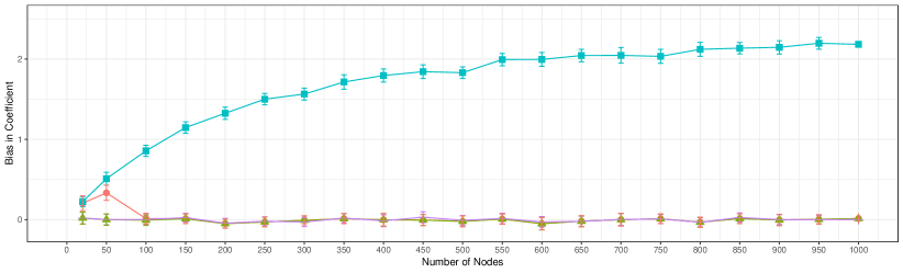
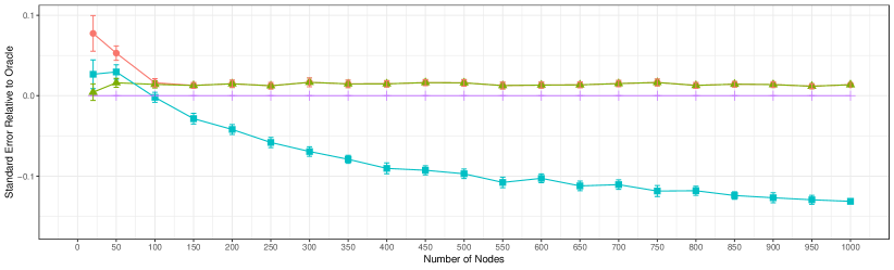
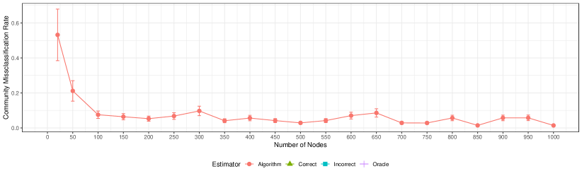
Figure 2: Comparison of the expected properties of the estimators where expectations is computed over $50$ random samples, allowing also for the formation of $95$% confidence intervals. The parameter of interest is sample size $n$, which varies, while the latent community model parameters remain fixed ($k=4,p_{\text{within}}=0.75,p_{\text{between}}=0.25$).

4.2 Simulation Results

In Figure 2, we observe how various outcomes of interest vary as the sample size (number of nodes) increases (while the latent community model parameters remain fixed at their reference values). We note that this simulation complies with our assumed setting and therefore our predictions (based on our theoretical results) of each estimator’s behavior should be consistent with what we observe. Let us begin by considering the first two plots, which show each estimator’s bias (top)—i.e., $\mathbb{E}\left[\hat{\beta}-\beta\right]$—and expected standard error relative to that of the Oracle estimator (middle)— $\mathbb{E}\left[\hat{\sigma}_{\hat{\beta}}-\hat{\sigma}_{\hat{\beta}_{Oracle}}\right]$— as a function of sample size. These plots confirm that the Oracle and Correct estimators are unbiased at all sample sizes, but the Correct estimator has larger variance, because it does not observe $X_{i}$. Additionally, the plots confirm that ignoring the latent community (as in the Incorrect estimator) leads to (omitted variable) bias at all sample sizes, which in our simulation amounts to a bias exceeding $2$ numerical units for $\beta$ in the limit. (Since the expected true value of $\beta$ across simulations, $\mathbb{E}\left[\beta\right]=0.1$, a bias of 2 units is a relative error of a remarkable $2,000\%$.) Beyond this extreme bias, the estimator, additionally, becomes overconfident in its (biased) estimation, which will lead to inaccurate confidence intervals and poor coverage probability. Finally, the plots confirm that the Algorithm estimator (based on estimated node locations) converges to the Correct estimator, and achieves consistent and (asymptotically) unbiased estimation of peer-influence.

Figure 2 also provides additional insight in the properties of the Algorithm estimator, in comparing it to the other estimators. Importantly, we observe that even at moderate sample sizes ($n=100$) the estimator appears to reach its asymptotic behavior (e.g., unbiasedness). Moreover, prior to reaching this asymptotic behavior, the Algorithm and Incorrect estimators have similar levels of bias, while the Algorithm estimator has larger variance. This implies that the biases resulting from omitting the node locations and using estimated locations (i.e. measurement error) are comparable, while the measurement error induces larger variance; therefore, at small sample sizes, the Incorrect estimator appears to provide a better estimation risk (with respect to loss in mean squared error). However, as sample size increases, the trade-off between these two sources of bias (and variance) begins to increasingly favor the measurement error, and the Algorithm estimator provides better estimation risk. We can see from the bottom plot in Figure 2 that the risk of the Algorithm estimator is, as expected, a function of the overall error in the node locations. Additionally, this estimator reaches its asymptotic behavior relatively quickly given the exponential decay in the measurement error.

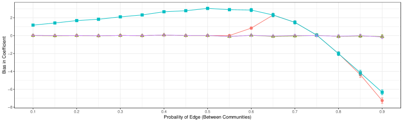
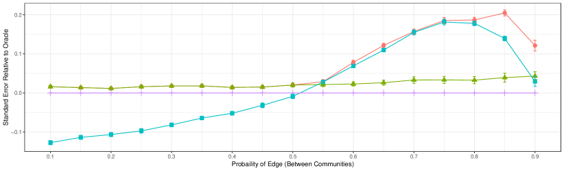
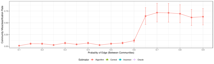
Figure 3: Comparison of the expected properties of the estimators where expectations is computed over $50$ random samples, allowing also for the formation of $95$% confidence intervals. The parameter of interest is $p_{\text{between}}$, which varies, while the sample size and other latent community model parameters remain fixed ($n=500,k=4,p_{\text{within}}=0.75$).

Assumption Violation

Although we are able to confirm our theoretical guarantees when our (sufficient) conditions are met, we also aim to explore the behavior of our estimator when these assumptions are violated. In Figure 3 we allow the probability of forming ties between nodes in different communities ($p_{\text{between}}$) to vary, and we capture the same three plots as before. As expected, when the between community ties probabilities are low, the Algorithm estimator, as before, has behavior equivalent to that of the Correct estimator. However, when the probability of between community exceeds $0.5$, we notice that the Algorithm begins to exhibit different behavior: both increased bias and variance. More specifically, we notice it converges to the behavior of the Incorrect estimator, indicating that the bias resulting from measurement error in the latent locations becomes as large as that resulting from the omission of the locations. The bottom plot in Figure 3 indicates that the Algorithm estimator’s degradation in behavior corresponds to its increase in latent location estimation error. The source of this error, can be explained by revisiting (5) as the bound it provides on the expected proportion of errors, includes the term $I=D_{\frac{1}{2}}\left(\text{Ber}\left(\frac{a}{n}\right)\|\text{Ber}\left(\frac{b}{n}\right)\right)$, where $\mathbb{E}\left[\frac{a}{n}\right]=p_{\text{between}}$. More specifically, $I=\left(a-b\right)^{2}/(an)$ up to a constant factor Zhang and Zhou (2016), therefore $I\rightarrow 0$ as $p_{\text{between}}\rightarrow p_{\text{within}}$, increasing the probability of location estimation errors.

Figure 3 also shows that when $p_{\text{between}}=p_{\text{within}}$ (at $0.75$) the biases of the Incorrect and Algorithm estimators are zero. At this point, the network is no longer homophilous (edges within and between communities are equally likely), implying that there are no longer arrows from $C_{i}$ and $C_{j}$ to $A_{ij}$ in the graphical causal model (Figure 1). As a result there is no longer a confounding backdoor pathway and there is no omitted variable bias. As $p_{\text{between}}$ increases beyond $p_{\text{within}}$, we see that the magnitude of the bias begins to increase again, but in the opposite direction. This is because the network is now increasingly heterophilous, and therefore $C_{i}$ and $C_{j}$ are increasingly more negatively correlated. We observe that both the bias and variance of the Algorithm estimator increases slightly beyond that of the Incorrect estimator, which is likely because the Algorithm’s assumption of homophily is violated, and therefore it is grouping precisely the wrong nodes together in a community. If there existed an approach that could achieve consistent identification of latent communities for heterophilous networks, consistent and (asymptotically) unbiased estimation of peer-influence can be obtained with similar arguments to those in our theoretical results.

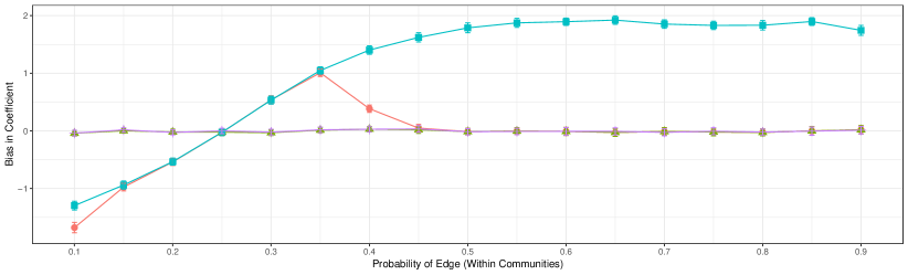
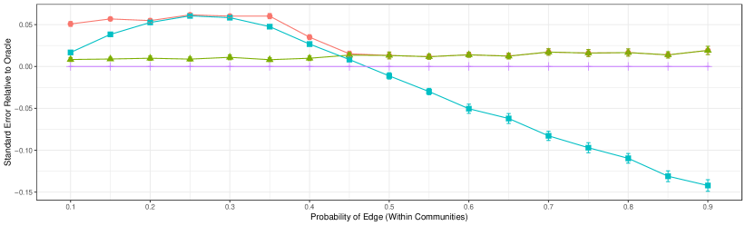
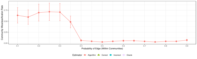
Figure 4: Comparison of the expected properties of the estimators where expectations is computed over $50$ random samples, allowing also for the formation of $95$% confidence intervals. The parameter of interest is sample size $p_{\text{within}}$, which varies, while the sample size and other latent community model parameters remain fixed ($n=500,k=4,p_{\text{between}}=0.25$).

In Figure 4 we allow the probability of forming ties between nodes in the same community ($p_{\text{within}}$) to vary, which leads to conclusions that are very similar to those for Figure 3 above, mutatis mutandis. The additional insight that we obtain from Figure 4, is that the increased bias and variance in the Incorrect and Algorithm estimators resulting from heterophily is smaller in magnitude than that in Figure 3. We suspect this is because, overall, the graph is more sparse in the heterophilous facets of Figure 4 (as compared to those in Figure 3); therefore, there is less potential for peer-influence, and the subsequent bias that results from its confoundment with homophily.

5 Discussion

We have shown that if a social network is generated by (a large class of) either latent community models or continuous latent space models, and the pattern of influence over that network then follows a linear model, it is possible to obtain consistent and asymptotically unbiased estimates of the social-influence parameter by controlling for estimates of the latent location of each node.

These are, to our knowledge, the first theoretical results which establish conditions under which social influence can be estimated from non-experimental data without confounding, even in the presence of latent homophily. Previous suggestions for providing such estimates by means of controlling for lagged observations (Valente, 2005) or matching (Aral et al., 2009) are in fact all invalid in the presence of latent homophily (Shalizi and Thomas, 2011). Instrumental variables which are also associated with network location have been proposed (Tucker, 2008); however, valid instruments are difficult to obtain and even more difficult to verify, as fundamentally their satisfaction of the exclusion restriction must be justified based on the specific context and argued from (behavioral) theory. An alternative to full identification is to provide partial identification (Manski, 2007), i.e., bounds on the range of the social-influence coefficient. VanderWeele (2011) provides such bounds under extremely strong parametric assumptions (among other things, $C_{i}$ must be binary and it must not interact with anything); Ver Steeg and Galstyan (2010); Ver Steeg and Galstyan (2013) provide non-parametric bounds, but must assume that each $Y_{i,t}$ evolves as a homogeneous Markov process, i.e., that there is no aging in the behavior of interest. None of these limitations apply to our approach.

Without meaning to diminish the value of our theoretical results, we feel it is also important to be clear about their limitations. The following assumptions were essential to our theoretical arguments:

1. The social network was generated exactly according to either a latent community model or a continuous latent space model.

2. We know whether it is a latent community model or a continuous latent space model.

3. We know either how many blocks there are (or how the number of blocks grows with $n$), or the latent space, its metric, and its link-probability function.

4. Fixed attributes of the nodes relevant to the behavior are either fully incorporated into the latent location, or stochastically independent of the location.

5. All of the relevant conditional expectation functions are linear.

To augment our theory with empirical results, we also conduct a simulation study specifically in the setting of networks generated according to a latent community model. We find that if locations are estimated with a (deterministic) minimax algorithm, our proposed estimator behaves as predicted by the theory, when all assumptions are satisfied. However, we also find that the theory is not fragile in the presence of small violations of the assumptions, e.g., the (asymptotic) bias in the estimation increases smoothly as the network formation process diverges from precisely a homophilous latent community. As a result, in practice, even if the assumptions are not (perfectly) satisfied the estimates should still exhibit bias reduction and (roughly) be “close” to the true parameter of interest.

We suspect—though we have no proofs—that similar theoretical and empirical results will hold for a somewhat wider class of well-behaved graphon network models. (Graphon estimation is an active topic of current research (Choi and Wolfe, 2014; Wolfe and Olhede, 2013), but it has focused on estimating the link-probability function $w$, rather than the latent locations $C$, though see Newman and Peixoto (2015) for a purely-heuristic treatment.) We also suspect such results will hold for nonlinear but smooth conditional-expectation functions quite generally. (The simulations of Worrall (2014) indicate that the approach works with at least some generalized linear models.) Additionally, it’s plausible that improved results can be achieved with these well-behaved graphon models, when a subset of the features relevant to tie formation (i.e., which impact node location) are observed. We however note that incorporating these features will require additional (careful) analysis, as any such feature may become redundant to $\hat{C}$ and have an undesirable impact on the statistical properties of the estimator. We also feel it is important to emphasize that there are many network processes which are perfectly well-behaved, and are even very natural, which fall outside the scope of our results; if, for instance, both ties $A_{ij}$ and behaviors $Y_{i,t}$ are influenced by a latent variable $C_{i}$ which has both continuous and discrete coordinates, there is no currently known way to consistently estimate the whole of $C_{i}$.

Despite these disclaimers, we wish to close by emphasizing the following point. In general, the strength of social influence cannot be estimated from observational social network data, because any feasible distribution over the observables can be achieved in infinitely many ways that trade off influence against latent homophily. What we have shown above is that if the network forms according to either of two standard models, and the rest of our assumptions hold, this result can be evaded, because the network itself makes all the relevant parts of the latent homophilous attributes manifest. To the best of our knowledge, this is the first situation in which the strength of social influence can be consistently estimated in the face of latent homophily—the first, but we hope not the last.

6 Proofs

See 1

Proof.

We are chiefly concerned with $\hat{\beta}_{OLS}$, the ordinary least squares estimate of $\beta$ in

$$Y_{i,t+1} =\alpha_{0}+\alpha_{1}Y_{i,t}+\beta\frac{\sum_{j}{\left(Y_{j,t}A_{ij}\right)}}{\sum_{j}{A_{ij}}}+\gamma_{0}^{T}\hat{C}_{i}+\overbrace{\epsilon_{i,t+1}+\gamma_{2}^{T}X_{i}+\left(\gamma_{1}^{T}C_{i}-\gamma_{0}^{T}\hat{C}_{i}\right)}^{\eta_{i,t+1}}$$

$$=\alpha_{0}+\alpha_{1}Y_{i,t}+\beta\frac{\sum_{j}{\left(Y_{j,t}A_{ij}\right)}}{\sum_{j}{A_{ij}}}+\gamma_{1}^{T}\hat{C}_{i}+\overbrace{\epsilon_{i,t+1}+\gamma_{2}^{T}X_{i}-\gamma_{1}^{T}\left(\hat{C}_{i}-C_{i}\right)}^{\eta_{i,t+1}},$$

where $\hat{C}_{i}$ is an estimated location for node $i$, $\eta_{i,t+1}$ is the (unobserved) noise term, and the equality follows from recognizing that $C=\hat{C}_{i}-\left(\hat{C}_{i}-C_{i}\right)$. By the assumption that $\mathrm{Pr}\left(C\neq\hat{C}\right)=0$, allowing for the replacement of $\hat{C}$ with $C$, this becomes

$$Y_{i,t+1}=\alpha_{0}+\alpha_{1}Y_{i,t}+\beta\frac{\sum_{j}{\left(Y_{j,t}A_{ij}\right)}}{\sum_{j}{A_{ij}}}+\gamma_{1}^{T}C_{i}+\overbrace{\epsilon_{i,t+1}+\gamma_{2}^{T}X_{i}}^{\eta_{i,t+1}}.$$

Given that $X_{i}\rotatebox{90.0}{$\models$}A_{ij},Y_{j,t}|C_{i},C_{j}$, we have $\mathrm{Cov}\left[\frac{\sum_{j}{\left(Y_{j,t}A_{ij}\right)}}{\sum_{j}{A_{ij}}},\eta_{i,t+1}\right]=0$ and therefore the OLS estimator for $\beta$ is unbiased and consistent. ∎

See 2

Proof.

First, recognize that

$$\mathrm{Cov}\left[\frac{\sum_{j}{\left(Y_{j,t}A_{ij}\right)}}{\sum_{j}{A_{ij}}},(\gamma_{1}^{T}C_{i}-\gamma_{0}^{T}\hat{C}_{i})\middle|A,Y_{i,t}\right]$$

$$~{}~{}~{}=\frac{\sum_{j}{A_{ij}\mathrm{Cov}\left[Y_{j,t},(\gamma_{1}^{T}C_{i}-\gamma_{0}^{T}\hat{C}_{i})\middle|A,Y_{i,t}\right]}}{\sum_{j}{A_{ij}}},$$ (8)

which follows from the linearity of covariance and the fact that $A$ is conditioned on (and therefore constant). Therefore, we consider the terms in the sum in the numerator:

$$\mathrm{Cov}\left[Y_{j,t},(\gamma_{1}^{T}C_{i}-\gamma_{0}^{T}\hat{C}_{i})|A,Y_{i,t}\right]$$ (9)

$$= \mathrm{Cov}\left[Y_{j,t},\gamma_{1}^{T}C_{i}|A,Y_{i,t}\right]$$

$$= \gamma_{1}^{T}\mathrm{Cov}\left[Y_{j,t},C_{i}|A,Y_{i,t}\right]$$ (10)

where (9) follows because we are conditioning on $A$ ($\hat{C}_{i}$ is a deterministic function of $A$) and additive constants do not change covariances. Additionally, (10) follows by linearity of covariance.

We are thus interested in the conditional covariance between $Y_{j,t}$ and $C_{i}$. We can at this point use the fact that (1) is a linear structural equation system. This allows us to use the Wright rules (Wright, 1934) to “read off” (conditional) covariances from the DAG corresponding to the structural equations (Moran, 1961). Briefly stated, to find the covariance between two variables $F$ and $G$ conditional on a set of variables $H$, these rules require us to (i) find all paths between $F$ and $G$ in the DAG, (ii) discard those paths which are “closed” when conditioning on $H$, (iii) multiply the linear regression coefficients encountered at each step along a path, (iv) multiply by a “source” variance for the common ancestor of all the variables along a path (conditional on $H$), when one exists, or (v) multiply by the conditional covariance of two “sources” linked by conditioning on a collider, and (vi) sum up over paths. (For the notion of a path in a DAG being “open” or “closed” when conditioning on a set of variables, see, e.g., Pearl (2009, Definition 1, p. 106).) Before presenting the relevant paths, it is convenient to introduce the abbreviation $d_{j}=\sum_{i}{A_{ij}}$ for the “degree” of node $j$, i.e., the number of social ties it has.

• Path: $Y_{j,t}\leftarrow C_{j}\rightarrow A_{ij}\leftarrow C_{i}$. Contribution: $\mathrm{Cov}\left[C_{i},C_{j}|A\right]\gamma_{1}$.

• Path: $Y_{j,t}\leftarrow Y_{j,t-1}\leftarrow Y_{i,t-2}\leftarrow C_{i}$. Contribution: $\alpha_{1}\frac{\beta A_{ij}}{d_{j}}\mathrm{Var}\left[C_{i}|A\right]\gamma_{1}$.

• Path: $Y_{j,t}\leftarrow Y_{j,t-1}\leftarrow Y_{j,t-2}\leftarrow Y_{i,t-3}\leftarrow C_{i}$. Contribution: $\alpha_{1}^{2}\frac{\beta A_{ij}}{d_{j}}\mathrm{Var}\left[C_{i}|A\right]\gamma_{1}$.

• Path: $Y_{j,t}\leftarrow Y_{j,t-1}\leftarrow\ldots\leftarrow Y_{j,t-h}\leftarrow Y_{i,t-h-1}\leftarrow C_{i}$. Contribution: $\alpha_{1}^{h}\frac{\beta A_{ij}}{d_{j}}\mathrm{Var}\left[C_{i}|A\right]\gamma_{1}$.

• Path: $Y_{j,t}\leftarrow Y_{i,t-2}\leftarrow\ldots\leftarrow Y_{i,t-h}\leftarrow C_{i}$. Contribution: $\frac{\beta A_{ij}}{d_{j}}\alpha_{1}^{h-2}\mathrm{Var}\left[C_{i}|A\right]\gamma_{1}$.

• Path: $Y_{j,t}\leftarrow Y_{l,t-1}\leftarrow C_{l}\rightarrow A_{li}\leftarrow C_{i}$. Contribution: $\frac{\beta A_{jl}}{d_{j}}\mathrm{Cov}\left[C_{l},C_{i}|A\right]\gamma_{1}$. (This must be summed over all possible nodes $l$.)

• Path: $Y_{j,t}\leftarrow Y_{j,t-1}\leftarrow Y_{l,t-2}\leftarrow C_{l}\rightarrow A_{li}\leftarrow C_{i}$. Contribution: $\alpha_{1}\frac{\beta A_{jl}}{d_{j}}\mathrm{Cov}\left[C_{l},C_{i}|A\right]\gamma_{1}$. (Similar paths extending back into the past add powers of $\alpha_{1}^{2},\alpha_{1}^{3}$, etc. This must also be summed over all possible nodes $l$.)

• Path: $Y_{j,t}\leftarrow Y_{l,t-1}\leftarrow Y_{l,t-2}\leftarrow C_{l}\rightarrow A_{li}\leftarrow C_{i}$. Contribution: $\alpha_{1}\frac{\beta A_{jl}}{d_{j}}\mathrm{Cov}\left[C_{l},C_{i}|A\right]\gamma_{1}$. (Similar paths extending back into the past add powers of $\alpha_{1}^{2},\alpha_{1}^{3}$, etc.)

From this enumeration, two things are clear: $1)$ all the paths lead to terms involve a single power of $\gamma_{1}$, and $2)$ every term involves a factor of either $\mathrm{Cov}\left[C_{j},C_{i}|A\right]$ or $\mathrm{Var}\left[C_{i}|A\right]$. Combining paths with the same source terms, we therefore have

$$\mathrm{Cov}\left[Y_{j,t},C_{i}|A,Y_{i,t}\right]$$

$$= \mathrm{Cov}\left[C_{i},C_{j}|A\right]\gamma_{1}$$

$$+\left(\sum_{h=1}^{T-1}{\alpha_{1}^{h}\frac{\beta A_{ij}}{d_{j}}}+\sum_{h=3}^{T-1}{\frac{\beta A_{ij}}{d_{j}}\alpha_{1}^{h-2}}\right)\mathrm{Var}\left[C_{i}|A\right]\gamma_{1}$$

$$+\sum_{l\neq i,j}{\left(\sum_{h=0}^{T-1}{\alpha_{1}^{h}(1+\alpha_{1})\frac{\beta A_{jl}}{d_{j}}}\right)\mathrm{Cov}\left[C_{l},C_{i}|A\right]}\gamma_{1}$$

$$= \mathrm{Cov}\left[C_{i},C_{j}|A\right]\gamma_{1}$$

$$+\xi_{ij}\mathrm{Var}\left[C_{i}|A\right]\gamma_{1}$$

$$+\sum_{l\neq i,j}{\zeta_{ijl}\mathrm{Cov}\left[C_{l},C_{i}|A\right]}\gamma_{1}$$

introducing $\xi_{ij}$ and $\zeta_{ijl}$ as the abbreviations for the appropriate sums. Substituting back into (10) amounts to multiplying every term here by $\gamma_{1}^{T}$ from the left. Substituting in turn into (8) yields the promised lemma. ∎

Remark: The form of the covariance $\mathrm{Cov}\left[Y_{j,t},C_{i}|A,Y_{i,t}\right]$ is somewhat complicated, because it turns out that many paths connect $Y_{j,t}$ and $C_{i}$. Most of these paths would, however, be closed if we also conditioned on $Y_{j,t-1}$ and $Y_{i,t-1}$. Conditioning on lagged values of $Y$ for both ego and alters in this way is sometimes done by practitioners, and would indeed leave open only the path $Y_{j,t}\leftarrow C_{j}\rightarrow A_{ij}\leftarrow C_{i}$. This would simplify the conditional covariance between $Y_{j,t}$ and $C_{i}$ to just $\gamma_{1}^{T}\mathrm{Cov}\left[C_{i},C_{j}|A\right]\gamma_{1}$. However, conditioning on these lagged values would mean altering the regression specification, and with it the coefficients and their interpretation. In particular, if autoregressive effects within nodes are strong, then $Y(j,t)$ and $Y(j,t-1)$ will be strongly correlated, which will introduce its own potential biases into the estimation of $\beta$. The net result may be to reduce the bias, but this would require detailed calculation. Since (as we show below) we are able to get consistent estimation of $\beta$ without introducing these lagged terms, we do not pursue this further here.

See 3

Proof.

First, we let $M_{n}=\sum_{i}^{n}{\mathbbm{1}\{\hat{C}_{i}\neq C_{i}\}}$, then from (4)–(5), we have

$$\mathbb{E}\left[M_{n}/n\right]\leq e^{-cn}$$

for an appropriate constant $c>0$ (and large enough $n$), which implies

$$\mathbb{E}\left[M_{n}\right]\leq ne^{-cn}.$$

We now turn our focus to the probability that $M\geq 1$:

$$\begin{split}\mathrm{Pr}\left(M_{n}\geq 1\right)&\leq\mathbb{E}\left[M_{n}\right]/1\quad(\text{Markov's Inequality})\\ &\leq ne^{-cn}\\ &=e^{-cn+\log{n}}\\ &=e^{-O(n)}.\end{split}$$

Therefore, the probability of making any latent location estimation errors at all goes to zero exponentially fast in $n$, and we note that it does so almost surely. Indeed, the almost sure convergence follows since $\sum_{n}{ne^{-cn}}$ is finite, and the Borel-Cantelli lemma (Grimmett and Stirzaker, 1992, Theorem 7.3.10a, p. 288) tells us that with probability $1$, $M_{n}\geq 1$ only finitely often, i.e., that $M_{n}\rightarrow 0$ almost surely. Therefore, with probability tending to one almost surely, as $n\rightarrow\infty$, $\hat{C}=C$. As a direct consequence, $\mathrm{Cov}\left[C_{i},C_{j}|\hat{C}_{i},\hat{C}_{j}\right]\xrightarrow{a.s.}0$. We note that although we have almost sure convergence in Lemma 3, only weaker consistency (convergence in probability) is required for the results that build atop this Lemma. ∎

See 4

Proof.

The second part of the lemma follows automatically from the first part, and the fact that assuming the GMZZ conditions means that the requirements of Lemma 3 are satisfied, implying that $\delta(n)=e^{-O(n)}$. Accordingly, we focus on establishing the first part of the lemma.

We now evoke the law of total covariance and decompose

$$\mathrm{Cov}\left[C_{i},C_{j}|A\right]$$ (11)

$$= \mathbb{E}\left[\mathrm{Cov}\left[C_{i},C_{j}|A,G_{n}\right]|A\right]+\mathrm{Cov}\left[\mathbb{E}\left[C_{i}|A,G_{n}\right],\mathbb{E}\left[C_{j}|A,G_{n}\right]|A\right],$$

where $G_{n}=1$ if all the nodes are assigned to their correct blocks (so $C_{i}=\hat{C}_{i}$ for all $i$) and $G_{n}=0$ otherwise. Given this decomposition, we will need to make a series of steps, dealing in turn with the expected covariance and the covariance of the expectations.

Step 1: Looking at the conditional covariance, we know

$$\mathbb{E}\left[\mathrm{Cov}\left[C_{i},C_{j}|A,G_{n}\right]|A\right]$$

$$= \mathrm{Pr}\left(G_{n}=1|A\right)\mathrm{Cov}\left[C_{i},C_{j}|A,G_{n}=1\right]+\mathrm{Pr}\left(G_{n}=0|A\right)\mathrm{Cov}\left[C_{i},C_{j}|A,G_{n}=0\right].$$

We also recognize that

$$\mathrm{Cov}\left[C_{i},C_{j}|A,G_{n}=1\right]=\mathrm{Cov}\left[\hat{C}_{i},\hat{C}_{j}|A,G_{n}=1\right]=0,$$

where the first equality follows from $G_{n}=1$ (i.e., $\hat{C}_{i}=C_{i}~{}\forall i$) and the second equality follows because $\hat{C}_{i}$ and $\hat{C}_{j}$ are functions $A$, which we condition on. Next we note that

$$\mathrm{Cov}\left[C_{i},C_{j}|A,G_{n}=0\right]\neq 0;$$

however, because $C_{i}$ and $C_{j}$ are “dummy” or indicator vectors, they are points on the corners of the $k-1$ dimensional simplex (or the origin). Moreover, $\mathrm{Cov}\left[C_{i},C_{j}|A,G_{n}=0\right]$ is a $k\times k$ covariance matrix, whose entries are bounded above by $1$ and below by $-1$. Therefore, the magnitude of $\lVert\mathrm{Cov}\left[C_{i},C_{j}|A,G_{n}=0\right]\rVert$ is bounded by a constant (with respect to $n$) whose value depends on the specific norm $\lVert\cdot\rVert$ used to measure magnitude. Therefore, combining the results for $G_{n}=1$ and $G_{n}=0$, we have

$$\mathbb{E}\left[\mathrm{Cov}\left[C_{i},C_{j}|A,G_{n}\right]|A\right]=0+O(\delta(n)).$$ (12)

Step 2: Turning to the conditional expectations, we similarly know that

$$\mathbb{E}\left[C_{i}|A,G_{n}=1\right]=\hat{C}_{i},$$ (13)

because when $G_{n}=1$, $\hat{C}_{i}=C_{i}~{}\forall i$. We can also define a new variable $\tilde{C}_{i}$ such that

$$\tilde{C}_{i}\equiv\mathbb{E}\left[C_{i}|A,G_{n}=0\right].$$ (14)

This new random variable $\tilde{C}_{i}$ is a function of $A$, and takes values within the interior of the convex hull of the $k-1$ dimensional simplex and the origin (rather than at the simplex’s corners and the origin). Because $G_{n}$ is an indicator variable, we can combine (13) and (14) to write

$$\mathbb{E}\left[C_{i}|A,G_{n}\right]=\hat{C}_{i}G_{n}+(1-G_{n})\tilde{C}_{i}$$ (15)

and similarly for $\mathbb{E}\left[C_{j}|A,G_{n}\right]$. Using (15) we can compute the covariance between the conditional expectations of the node locations:

$$\mathrm{Cov}\left[\mathbb{E}\left[C_{i}|A,G_{n}\right],\mathbb{E}\left[C_{j}|A,G_{n}\right]|A\right]$$

$$= \mathrm{Cov}\left[\hat{C}_{i}G_{n}+\tilde{C}_{i}(1-G_{n}),\hat{C}_{j}G_{n}+\tilde{C}_{j}(1-G_{n})|A\right]$$

$$= \mathrm{Cov}\left[\hat{C}_{i}G_{n},\hat{C}_{j}G_{n}|A\right]+\mathrm{Cov}\left[\tilde{C}_{i}(1-G_{n}),\tilde{C}_{j}(1-G_{n})|A\right]$$

$$+\mathrm{Cov}\left[\hat{C}_{i}G_{n},\tilde{C}_{j}(1-G_{n})|A\right]+\mathrm{Cov}\left[\tilde{C}_{i}(1-G_{n}),\hat{C}_{j}G_{n}|A\right]$$

$$= \hat{C}_{i}\mathrm{Var}\left[G_{n}|A\right]\hat{C}_{j}^{T}+\tilde{C}_{i}\mathrm{Var}\left[1-G_{n}|A\right]\tilde{C}_{j}^{T}$$

$$+\hat{C}_{i}\mathrm{Cov}\left[G_{n},1-G_{n}|A\right]\tilde{C}_{j}^{T}+\tilde{C}_{i}\mathrm{Cov}\left[1-G_{n},G_{n}|A\right]\hat{C}_{j}^{T}$$

$$= O\left(\mathrm{Var}\left[G_{n}|A\right]\right)+O\left(\mathrm{Var}\left[1-G_{n}|A\right]\right)$$

$$+O\left(\mathrm{Cov}\left[G_{n},1-G_{n}|A\right]\right)+O\left(\mathrm{Cov}\left[1-G_{n},G_{n}|A\right]\right)$$

$$= O(\delta(n)).$$ (18)

(6) follows from the fact that the four vectors —$\hat{C}_{i},\tilde{C}_{i},\hat{C}_{j}$ and $\tilde{C}_{j}$—are all functions of $A$ and therefore conditionally constant. Moreover, (6) follows from the fact that these vectors all lie within the convex hull of the $k-1$ dimensional simplex and the origin, and therefore their outer products—$\hat{C}_{i}\hat{C}_{j}^{T}$, $\tilde{C}_{i}\tilde{C}_{j}^{T}$, $\hat{C}_{i}\tilde{C}_{j}^{T}$ and $\tilde{C}_{i}\hat{C}_{j}^{T}$—are also bounded by a constant (with respect to $n$). Finally, (18) follows from two realizations. First, that $1-G_{n}$ is a binary variable whose expectation is $O(\delta(n))$, so $\mathrm{Var}\left[1-G_{n}|A\right]=\mathrm{Var}\left[G_{n}|A\right]=\delta(n)(1-\delta(n))=O(\delta(n))$. Secondly, since $G_{n}(1-G_{n})=0$ always, $\mathrm{Cov}\left[G_{n},1-G_{n}|A\right]=\mathbb{E}\left[G_{n}(1-G)_{n}|A\right]-\mathbb{E}\left[G_{n}|A\right]\mathbb{E}\left[1-G_{n}|A\right]=-(1-\delta(n))\delta(n)=O(\delta(n))$.

Thus plugging (12) and (18) into (11), we have

$$\mathrm{Cov}\left[C_{i},C_{j}|A\right]=O(\delta(n))+O(\delta(n))=O(\delta(n))$$

∎

Lemma 5.

Suppose that the assumptions from Section 2 hold, the network forms according to a latent community model, and $\hat{C}$ can be estimated with error rate $\delta(n)$. Then $\mathrm{Var}\left[C_{i}|A\right]=O(\delta(n))$. If the latent community model also satisfies the GMZZ conditions and a minimax algorithm is used to estimate $\hat{C}$, then $\mathrm{Var}\left[C_{i}|A\right]=e^{-O(n)}$.

Proof.

The proof runs along the same lines as that of Lemma 4, albeit with somewhat less algebra, and so only sketched. We can write $\mathrm{Var}\left[C_{i}|A\right]=\mathbb{E}\left[\mathrm{Var}\left[C_{i}|A,G_{n}\right]|A\right]+\mathrm{Var}\left[\mathbb{E}\left[C_{i}|A,G_{n}\right]|A\right]$. $\mathrm{Var}\left[C_{i}|A,G_{n}=1\right]=0$, because, conditional on $G_{n}=1$, $C_{i}=\hat{C_{i}}$ which is a function of $A$. If $G_{n}=0$, however, the variance of $C_{i}$ is bounded, since every possible value of $C_{i}$ is a corner on the simplex (or the origin), hence $\mathbb{E}\left[\mathrm{Var}\left[C_{i}|A,G_{n}\right]|A\right]=O(\delta(n))$. Similarly, $\mathbb{E}\left[C_{i}|A,G_{n}=1\right]=\hat{C}_{i}$, which is constant (conditional on $A$) and does not contribute to the conditional-on-$A$ variance, while $\mathbb{E}\left[C_{i}|A,G_{n}=0\right]$, which is random with respect to $A$, is still bounded within the convex hull of the simplex and the origin. Thus $\mathrm{Var}\left[C_{i}|A\right]=O(\delta(n))$ over-all. Further assuming the GMZZ conditions tells us $\delta(n)=e^{-O(n)}$. ∎

See 1

Proof.

As in Lemma 1, we are again chiefly concerned with $\hat{\beta}_{OLS}$, the ordinary least squares estimate of $\beta$ in

$$Y_{i,t+1}=\alpha_{0}+\alpha_{1}Y_{i,t}+\beta\frac{\sum_{j}{\left(Y_{j,t}A_{ij}\right)}}{\sum_{j}{A_{ij}}}+\gamma_{0}^{T}\hat{C}_{i}+\overbrace{\epsilon_{i,t+1}+\gamma_{2}^{T}X_{i}+\left(\gamma_{1}^{T}C_{i}-\gamma_{0}^{T}\hat{C}_{i}\right)}^{\eta_{i,t+1}}$$ (19)

where $\hat{C}_{i}$ is an estimated location for node $i$, $\eta_{i,t+1}$ is the (unobserved) noise term. Moreover, we know that

$$\mathbb{E}\left[\hat{\beta}_{OLS}\middle|A\right] =\beta+O\left(\mathrm{Cov}\left[\frac{\sum_{j}{\left(Y_{j,t}A_{ij}\right)}}{\sum_{j}{A_{ij}}},\eta_{i,t+1}\right]\middle|A\right)$$ (20)

$$=\beta+O\left(\mathrm{Cov}\left[\frac{\sum_{j}{\left(Y_{j,t}A_{ij}\right)}}{\sum_{j}{A_{ij}}},\left(\gamma_{1}^{T}C_{i}-\gamma_{0}^{T}\hat{C}_{i}\right)\right]\middle|A\right)$$ (21)

$$=\beta+O\left(\gamma_{1}^{T}\mathrm{Cov}\left[C_{i},C_{j}|A\right]\gamma_{1}\right)+O\left(\gamma_{1}^{T}\mathrm{Var}\left[C_{i}|A\right]\gamma_{1}\right)+O\left(\gamma_{1}^{T}\mathrm{Cov}\left[C_{i},C_{l}|A\right]\gamma_{1}\right)$$ (22)

$$=\beta+O\left(\delta(n)\right)$$ (23)

where (20) follows from the definition of the OLS estimate for $\beta$ in (19), (21) follows from the assumptions of the setting (chiefly (3)), (22) follows from Lemma 2, and finally (23) follows from Lemmas 4 and 5. Moreover we have that $O\left(\delta(n)\right)$ can be made exponentially small, and in only a polynomial cost in computational time, (§2.2 above). Therefore, the bias in $\hat{\beta}_{OLS}$ is itself exponentially small in $n$. Hence $\hat{\beta}_{OLS}$ will be asymptotically unbiased and consistent as $n\rightarrow\infty$. ∎

See 2

Proof.

As in the proof of Theorem 1, it will be enough to show that both $\mathrm{Cov}\left[C_{i},C_{j}|A\right]\rightarrow 0$ and $\mathrm{Var}\left[C_{i}|A\right]\rightarrow 0$. To do so, we showed that $\mathrm{Cov}\left[C_{i},C_{j}|A\right]$ and $\mathrm{Var}\left[C_{i}|A\right]$ were both $O(\delta(n))$, where $\delta(n)$ was the probability of community discovery mis-labeling any nodes at all. We cannot expect such exact recovery of the latent variables in a continuous model, so we will work instead with $\delta(\epsilon_{n},n)$, the probability that all estimated positions are within $\epsilon_{n}$ of the true positions, and let $\epsilon_{n}\rightarrow 0$ at a suitable rate.

To be specific, define $\delta(n,\epsilon)$ as $\mathrm{Pr}\left(\max_{i\in 1:n}{\|C_{i}-\hat{C}_{i}\|\geq\epsilon}\right)$, where $\hat{C}_{i}$ is the maximum likelihood estimate of $C_{i}$. By (7)

$$\delta(n,\epsilon)\leq\mathcal{N}(n,\epsilon)e^{-\kappa\epsilon n^{2}}$$

where $\mathcal{N}(n,\epsilon)$ is polynomial in both $n$ and in $1/\epsilon$. Now fix a sequence $\epsilon_{n}>0$ such that $\epsilon_{n}\rightarrow 0$ as $n\rightarrow\infty$, while $\epsilon_{n}n^{2}\rightarrow\infty$ at least polynomially fast in $n$. (For instance, but not necessarily optimally, $\epsilon_{n}=n^{-1}$.) We will now show that $\mathrm{Cov}\left[C_{i},C_{j}|A\right]$ and $\mathrm{Var}\left[C_{i}|A\right]$ are both $O(\epsilon_{n}^{2})+O(\delta(n,\epsilon_{n}))$, which, under these conditions, is polynomial in $1/n$.

We need to modify one more definition from the stochastic block model case: we re-define $G_{n}$ as the indicator for the event that $\max_{i\in 1:n}{\|C_{i}-\hat{C}_{i}\|<\epsilon_{n}}$. (Thus $G_{n}=1$ with probability $1-\delta(n,\epsilon_{n})$.) With this in place, we can now proceed much as in Lemma 4: by the law of total covariance,

$$\mathrm{Cov}\left[C_{i},C_{j}|A\right]$$

$$= \mathbb{E}\left[\mathrm{Cov}\left[C_{i},C_{j}|A,G_{n}\right]|A\right]+\mathrm{Cov}\left[\mathbb{E}\left[C_{i}|A,G_{n}\right],\mathbb{E}\left[C_{j}|A,G_{n}\right]|A\right].$$

If $G_{n}=1$, then $C_{i}=\hat{C}_{i}+O(\epsilon_{n})$ and $C_{j}=\hat{C}_{j}+O(\epsilon_{n})$, consequently $\mathrm{Cov}\left[C_{i},C_{j}|A,G_{n}=1\right]=O(\epsilon_{n}^{2})$. If, on the other hand, $G_{n}=0$, we do not have such nice control over the covariance of the true locations, but the fact that they lie in a compact set means that there is an upper bound, independent of $n$, on the magnitude of their covariance. So we have shown that

$$\mathbb{E}\left[\mathrm{Cov}\left[C_{i},C_{j}|A,G_{n}\right]|A\right]$$ (24)

$$= O(1-\delta(n,\epsilon_{n}))O(\epsilon_{n}^{2})+O(\delta(n,\epsilon_{n}))O(1)$$

$$= O(\epsilon_{n}^{2})+O(\delta(n,\epsilon_{n})).$$

Turning to the conditional expectations,

$$\mathbb{E}\left[C_{i}|A,G_{n}=1\right]=\hat{C}_{i}+O(\epsilon_{n})$$

and we may define

$$\tilde{C}_{i}\equiv\mathbb{E}\left[C_{i}|A,G_{n}=0\right]$$

which is a function of $A$, and takes values in the convex hull of the compact set which supports the distribution of $C_{i}$. Thus

$$\mathbb{E}\left[C_{i}|A,G_{n}\right]=G_{n}\hat{C}_{i}+G_{n}O(\epsilon_{n})+(1-G_{n})\tilde{C}_{i}.$$

Continuing to imitate the proof of Lemma 4,

$$\mathrm{Cov}\left[\mathbb{E}\left[C_{i}|A,G_{n}\right],\mathbb{E}\left[C_{j}|A,G_{n}\right]|A\right]$$

$$= \mathrm{Cov}\left[G_{n}\hat{C}_{i}+G_{n}O(\epsilon_{n})+(1-G_{n})\tilde{C}_{i},G_{n}\hat{C}_{j}+G_{n}O(\epsilon_{n})+(1-G_{n})\tilde{C}_{j}|A\right]$$

$$= \mathrm{Var}\left[G_{n}|A\right](\hat{C}_{i}\hat{C}_{j}^{T}+\hat{C}_{i}O(\epsilon_{n})+O(\epsilon_{n})\hat{C}_{j}^{T}+O(\epsilon_{n}^{2}))$$

$$+\mathrm{Var}\left[1-G_{n}|A\right]\tilde{C}_{i}\tilde{C}_{j}^{T}$$

$$\mathrm{Cov}\left[G_{n},1-G_{n}|A\right](\hat{C}_{i}\tilde{C}_{j}^{T}+O(\epsilon_{n})\tilde{C}_{j}^{T}+\tilde{C}_{i}\hat{C}_{j}^{T}+\tilde{C}_{i}O(\epsilon_{n})).$$

By an argument just like the one used in Lemma 4, $\mathrm{Var}\left[G_{n}|A\right]=\mathrm{Var}\left[1-G_{n}|A\right]=O(\delta(n,\epsilon_{n}))$, and likewise $\mathrm{Cov}\left[G_{n},1-G_{n}|A\right]=O(\delta(n,\epsilon_{n}))$. On the other hand, $\hat{C}_{i}$ and $\tilde{C}_{i}$ are both $O(1)$. Thus

$$\mathrm{Cov}\left[\mathbb{E}\left[C_{i}|A,G_{n}\right],\mathbb{E}\left[C_{j}|A,G_{n}\right]|A\right]$$ (25)

$$= O(\delta(n,\epsilon_{n}))+O(\epsilon_{n}\delta(n,\epsilon_{n}))+O(\epsilon_{n}^{2}\delta(n,\epsilon_{n}))$$

$$= O(\delta(n,\epsilon_{n}))$$

since $\epsilon_{n}\rightarrow 0$.

Combining (24) with (25),

$$\mathrm{Cov}\left[C_{i},C_{j}|A\right]$$ (26)

$$= \mathbb{E}\left[\mathrm{Cov}\left[C_{i},C_{j}|A,G_{n}\right]|A\right]+\mathrm{Cov}\left[\mathbb{E}\left[C_{i}|A,G_{n}\right],\mathbb{E}\left[C_{j}|A,G_{n}\right]|A\right]$$

$$= O(\epsilon_{n}^{2})+O(\delta(n,\epsilon_{n}))+O(\delta(n,\epsilon_{n}))$$

$$= O(\epsilon_{n}^{2})+O(\delta(n,\epsilon_{n})).$$

A careful inspection of the preceding steps show that none of them assumed that $i\neq j$. We may therefore conclude that

$$\mathrm{Var}\left[C_{i}|A\right]=\mathrm{Cov}\left[C_{i},C_{i}|A\right]=O(\epsilon_{n}^{2})+O(\delta(n,\epsilon_{n}))$$

Since the bias is $O(\mathrm{Cov}\left[C_{i},C_{j}|A\right])+O(\mathrm{Var}\left[C_{i}|A\right])$, the bias is $O(\epsilon_{n}^{2})+O(\delta(n,\epsilon_{n}))$. At the corresponding part of the proof of Theorem 1, we had a bias that was $O(\delta(n))$, and an invocation of the GMZZ conditions showed that this must be exponentially small in $n$. Here, we need to show that $\epsilon_{n}^{2}\rightarrow 0$ and that $\delta(n,\epsilon_{n})\rightarrow 0$ as well. Invoking the Asta conditions lets us say that

$$\delta(n,\epsilon_{n})\leq\mathcal{N}(n,\epsilon_{n})exp{(-\kappa\epsilon_{n}n^{2})}$$

so it’s enough to have the right-hand side of this equation approaching zero. Since the function $\mathcal{N}(n,\epsilon)$ is polynomial in $n$ and $1/\epsilon$, we can say that

$$\log{\delta(n,\epsilon)}=O(\log{n}-\log{\epsilon_{n}}+\epsilon_{n}n^{2})$$

From this, it’s clear that so long as $\epsilon_{n}n^{2}\rightarrow\infty$ at some polynomial rate, $\delta(n,\epsilon_{n})$ will be exponentially small in some power of $n$, and $\mathrm{Cov}\left[C_{i},C_{j}|A\right]$ will be dominated by the $O(\epsilon_{n}^{2})$ term, which will be polynomial in $n$.

In particular, if $\epsilon_{n}\propto n^{-r}$, for $0<r<2$, then $\mathcal{N}(n,\epsilon_{n})$ is still polynomial in $n$, but $\exp{(-\kappa\epsilon_{n}n^{2})}=\exp{(-\kappa^{\prime}n^{2-r})}$, so over-all $\delta(n,\epsilon_{n})$ goes to zero exponentially fast in some power of $n$. Thus we can get $\mathrm{Cov}\left[C_{i},C_{j}|A\right]=O(n^{-2r})$ for any $r<2$.

Having established that both $\mathrm{Cov}\left[C_{i},C_{j}|A\right]$ and $\mathrm{Var}\left[C_{i}|A\right]$ are, at most, $O(n^{-2r})$, reasoning as in the proof of Theorem 1 shows that the bias, too, is $O(n^{-2r})$, for some $r<2$. ∎

Note: Attempting to optimize the rate at which $\mathrm{Cov}\left[C_{i},C_{j}|A\right]\rightarrow 0$, by differentiating (26) with respect to $\epsilon_{n}$ and setting the derivative to zero, leads to an un-illuminating transcendental equation, which we omit, because the over-all convergence rate is still polynomial in $n$.

Acknowledgments

We thank Andrew C. Thomas, David S. Choi, and Veronica Marotta for many valuable discussions on these and related ideas over the years. We thank Dena Asta and Hannah Worrall, for sharing Asta (2015) and Worrall (2014), respectively; Chao Gao, Zongming Ma, Anderson Y. Zhang, and Harrison H. Zhou for sharing code related to Gao et al. (2017); Oleg Sofrygin for assistance with simulations using Sofrygin et al. (2017); and Max Kaplan for related programming assistance. CRS was supported during this work by grants from the NSF (DMS1207759 and DMS1418124) and the Institute for New Economic Thinking (INO1400020) and EM was supported during this work by a grant from Facebook (Computational Social Science Methodology Research Awards).

References

- Aral et al. (2009) Sinan Aral, Lev Muchnik, and Arun Sundararajan. Distinguishing influence based contagion from homophily driven diffusion in dynamic networks. Proceedings of the National Academy of Sciences (USA), 106:21544–21549, 2009. doi: 10.1073/pnas.0908800106.
- Asta (2015) Dena Marie Asta. Geometric Approaches to Inference: Non-Euclidean Data and Networks. PhD thesis, Carnegie Mellon University, 2015.
- Bickel and Chen (2009) Peter J. Bickel and Aiyou Chen. A nonparametric view of network models and Newman-Girvan and other modularities. Proceedings of the National Academy of Sciences (USA), 106:21068–21073, 2009. doi: 10.1073/pnas.0907096106.
- Brannan et al. (1999) David A. Brannan, Matthew F. Esplen, and Jeremy J. Gray. Geometry. Cambridge University Press, Cambridge, England, 1999.
- Choi and Wolfe (2014) David S. Choi and Patrick J. Wolfe. Co-clustering separately exchangeable network data. Annals of Statistics, 42:29–63, 2014. doi: 10.1214/13-AOS1173. URL http://arxiv.org/abs/1212.4093.
- Christakis and Fowler (2007) Nicholas A. Christakis and James H. Fowler. The spread of obesity in a large social network over 32 years. The New England Journal of Medicine, 357:370–379, 2007. URL http://content.nejm.org/cgi/content/abstract/357/4/370.
- Csardi and Nepusz (2006) Gabor Csardi and Tamas Nepusz. The igraph software package for complex network research. InterJournal, Complex Systems:1695, 2006. URL https://igraph.org.
- Davin et al. (2014) Joseph P. Davin, Sunil Gupta, and Mikolaj Jan Piskorski. Separating homophily and peer influence with latent space. Technical Report Working Paper 14-053, Harvard Business School, 2014. URL http://hbswk.hbs.edu/item/separating-homophily-and-peer-influence-with-latent-space.
- DuBois et al. (2013) Christopher DuBois, Carter Butts, and Padhraic Smyth. Stochastic blockmodeling of relational event dynamics. In Carlos M. Carvalho and Pradeep Ravikumar, editors, Sixteenth International Conference on Artificial Intelligence and Statistics [AISTATS 2013], pages 238–246, 2013. URL http://jmlr.org/proceedings/papers/v31/dubois13a.html.
- Fortunato (2010) Santo Fortunato. Community detection in graphs. Physics Reports, 486:75–174, 2010. URL http://arxiv.org/abs/0906.0612.
- Gao et al. (2017) Chao Gao, Zongming Ma, Anderson Y. Zhang, and Harrison H. Zhou. Achieving optimal misclassification proportion in stochastic block models. Journal of Machine Learning Research, 18(60):1–45, 2017. URL http://jmlr.org/papers/v18/16-245.html.
- Ghasemian et al. (2015) Amir Ghasemian, Pan Zhang, Aaron Clauset, Cristopher Moore, and Leto Peel. Detectability thresholds and optimal algorithms for community structure in dynamic networks. arxiv:1506.06179, 2015. URL http://arxiv.org/abs/1506.06179.
- Girvan and Newman (2002) Michelle Girvan and Mark E. J. Newman. Community structure in social and biological networks. Proceedings of the National Academy of Sciences (USA), 99:7821–7826, 2002. URL http://arxiv.org/abs/cond-mat/0112110.
- Grimmett and Stirzaker (1992) G. R. Grimmett and D. R. Stirzaker. Probability and Random Processes. Oxford University Press, Oxford, 2nd edition, 1992.
- Hoff et al. (2002) Peter D. Hoff, Adrian E. Raftery, and Mark S. Handcock. Latent space approaches to social network analysis. Journal of the American Statistical Association, 97:1090–1098, 2002. URL http://www.stat.washington.edu/research/reports/2001/tr399.pdf.
- Kallenberg (2005) Olav Kallenberg. Probabilistic Symmetries and Invariance Principles. Springer-Verlag, New York, 2005.
- Leenders (1995) Roger Th. A. J. Leenders. Structure and Influence: Statistical Models for the Dynamics of Actor Attributes, Network Structure and Their Interdependence. Thesis Publishers, Amsterdam, 1995.
- Manski (2007) Charles F. Manski. Identification for Prediction and Decision. Harvard University Press, Cambridge, Massachusetts, 2007.
- Martin (2009) John Levi Martin. Social Structures. Princeton University Press, Princeton, New Jersey, 2009.
- Moran (1961) P. A. P. Moran. Path coefficients reconsidered. Australian Journal of Statistics, 3:87–93, 1961. doi: 10.1111/j.1467-842X.1961.tb00314.x.
- Newman and Peixoto (2015) Mark E. J. Newman and Tiago P. Peixoto. Generalized communities in networks. Physical Review Letters, 115:088701, 2015. doi: 10.1103/PhysRevLett.115.088701. URL http://arxiv.org/abs/1505.07478.
- Pearl (2009) Judea Pearl. Causal inference in statistics: An overview. Statistics Surveys, 3:96–146, 2009. URL http://projecteuclid.org/euclid.ssu/1255440554.
- R Core Team (2020) R Core Team. R: A Language and Environment for Statistical Computing. R Foundation for Statistical Computing, Vienna, Austria, 2020. URL http://www.R-project.org. ISBN 3-900051-07-0.
- Rényi (1961) Alfréd Rényi. On measures of entropy and information. In Jerzy Neyman, editor, Proceedings of the Fourth Berkeley Symposium on Mathematical Statistics and Probability, volume 1, pages 547–561, Berkeley, 1961. University of California Press. URL https://projecteuclid.org/euclid.bsmsp/1200512181.
- Richardson and Robins (2013) Thomas S. Richardson and James M. Robins. Single world intervention graphs (SWIGs): A unification of the counterfactual and graphical approaches to causality. Technical Report 128, Center for Statistics and the Social Sciences, University of Washington, 2013. URL http://www.csss.washington.edu/Papers/wp128.pdf.
- Sarkar and Moore (2006) Purnamrita Sarkar and Andrew W. Moore. Dynamic social network analysis using latent space models. In Yair Weiss, Bernhard Schölkopf, and John C. Platt, editors, Advances in Neural Information Processing Systems 18 (NIPS 2005), pages 1145–1152, Cambridge, Massachusetts, 2006. MIT Press. URL http://books.nips.cc/papers/files/nips18/NIPS2005_0724.pdf.
- Schweinberger and Luna (2018) Michael Schweinberger and Pamela Luna. hergm: Hierarchical exponential-family random graph models. Journal of Statistical Software, 85(1):1–39, 2018. doi: 10.18637/jss.v085.i01.