About AGN ionization echoes, thermal echoes, and ionization deficits in low redshift Lyman-$\alpha$ blobs

Abstract

We report the discovery of 14 Lyman-$\alpha$ blobs (LABs) at $z\sim 0.3$, existing at least $4-7$ billion years later in the Universe than all other LABs known. Their optical diameters are $20-70$ kpc, and GALEX data imply Ly $\alpha$ luminosities of $(0.4-6.3)\times 10^{43}$ erg s^-1. Contrary to high-z LABs, they live in low-density areas. They are ionized by AGN, suggesting that cold accretion streams as a power source must deplete between $z=2$ and $z=0.3$. We also show that transient AGN naturally explain the ionization deficits observed in many LABs: Their Ly $\alpha$ and X-ray fluxes decorrelate below $\lesssim 10^{6}$ years because of the delayed escape of resonantly scattering Ly $\alpha$ photons. High Ly $\alpha$ luminosities do not require currently powerful AGN, independent of obscuration. Chandra X-ray data reveal intrinsically weak AGN, confirming the luminous optical nebulae as impressive ionization echoes. For the first time, we also report mid-infrared thermal echoes from the dusty tori. We conclude that the AGN have faded by $3-4$ orders of magnitude within the last $10^{4-5}$ years, leaving fossil UV, optical and thermal radiation behind. The host galaxies belong to the group of previously discovered Green Bean galaxies (GBs). Gemini optical imaging reveals smooth spheres, mergers, spectacular outflows and ionization cones. Because of their proximity and high flux densities, GBs are perfect targets to study AGN feedback, mode switching and the Ly $\alpha$ escape. The fully calibrated, coadded optical FITS images are publicly available.

1 Introduction

Lyman-$\alpha$ blobs (LABs) are extended Ly $\alpha$ nebulae with luminosities of $L_{\rm Ly\,\alpha}=10^{42-44}$ erg s^-1, populating the Universe at $z\gtrsim 2$. They are often selected using optical narrow-band filters that isolate redshifted Ly $\alpha$ emission (e.g. Kodaira et al., 2003; Matsuda et al., 2004, 2011; Dey et al., 2005; Ouchi et al., 2009; Yang et al., 2009, 2010). LABs are $20-200$ kpc in size and show a bewildering range of properties. They can be associated with Lyman Break Galaxies (Steidel et al., 1995), visible and obscured AGN, starburst sub-mm galaxies and passively evolving red galaxies (e.g. Francis et al., 2001; Chapman et al., 2004; Matsuda et al., 2004; Geach et al., 2009; Webb et al., 2009).

LABs are landmarks of ongoing massive galaxy formation (Matsuda et al., 2006; Prescott et al., 2008), yet the ionizing sources in many of them remain mysterious. Our understanding of these processes would greatly benefit from studying the physical conditions in LABs. However, this is difficult as (1) cosmological surface brightness dimming reduces the flux densities by factors $\gtrsim 100$, (2) the Ly $\alpha$ line is resonant, and (3) non-resonant optical lines are redshifted into and beyond the near-infrared atmospheric passbands. The resonant character of Ly $\alpha$ causes two main problems with the interpretation of Ly $\alpha$ data.

First, Ly $\alpha$ photons scatter efficiently in space and frequency when propagating through a moving medium. Three-dimensional radiative transfer calculations (e.g. Meinköhn & Richling, 2002; Verhamme et al., 2006; Kollmeier et al., 2010) reveal a great variety of double-peaked Ly $\alpha$ line profiles emerging for various static and kinematic source/halo configurations (for a one-dimensional analytic description in a static medium see Neufeld, 1990). It is difficult at best to infer the gas kinematics and the Ly $\alpha$ production sites from Ly $\alpha$ imaging and spectroscopy alone. A multi-wavelength perspective is required, including optically thin lines such as [O iii] and H $\alpha$ (e.g. Saito et al., 2008; Weijmans et al., 2010; Yang et al., 2011a, 2014; Martin et al., 2014; Zabl et al., 2015; Swinbank et al., 2015).

The second problem is that we need to understand the processes that govern how many Ly $\alpha$ photons manage to escape, so that they become observable at all. Dust, neutral hydrogen, metallicity and gas outflows control this escape fraction. The latter can range from less than 1 per cent to more than 50 per cent (Yang et al., 2015, and references therein). Intrinsically, the H $\alpha$/Ly $\alpha$ line ratio is fixed for a photo-ionized nebula in equilibrium; the H $\alpha$ line can then be used to estimate the escape fraction and the total amount of Ly $\alpha$ produced. However, it is only for a small redshift window of $z=1.9-2.4$ that both lines are observable from the ground. Worse, AGN variability may change the escape fraction further, by orders of magnitude, due to delayed Ly $\alpha$ escape (Roy et al., 2010; Xu et al., 2011).

Probably the largest mystery with LABs is their frequent lack of ionizing sources; some LABs show no continuum counterparts at all. The lack of accessible diagnostic lines has prevented consistent conclusions on many occasions, and various processes have been suggested that could power LABs. For example, LABs are preferentially found in denser areas and filaments (Saito et al., 2008; Yang et al., 2010; Erb et al., 2011; Matsuda et al., 2011), where LABs easily accrete cold neutral hydrogen from the cosmic web (Haiman et al., 2000; Dijkstra & Loeb, 2009; Goerdt et al., 2010). This is a requirement by $\Lambda$CDM galaxy formation models. The Ly $\alpha$ emission arises because of collisional excitation of hydrogen (virial temperature of $10^{4-5}$ K) when it sinks into the dark matter haloes. It can contribute to an LAB’s ionization over $10-30$ per cent of the Hubble time (Dijkstra & Loeb, 2009). Some calculations including self-shielding and realistic gas phases indicate that cold accretion alone could be insufficient to explain the Ly $\alpha$ fluxes of luminous LABs (Faucher-Giguère et al., 2010). On the other hand, Rosdahl & Blaizot (2012) and Cen & Zheng (2013) find cold streams to be rather powerful, reproducing the size–luminosity function of observed LABs. The challenges in modelling the cold streams are mirrored on the observational side. One such gravitationally powered LAB (Nilsson et al., 2006) is questioned by Prescott et al. (2015), who discovered an embedded obscured AGN and argue that the original data speak against cold accretion.

Alternatively, LABs can be shock-ionized by starburst-driven superwinds (Taniguchi & Shioya, 2000), and photoionized by obscured AGN or starbursts (e.g. Chapman et al., 2001; Geach et al., 2009). Starbursts alone cannot explain Ly $\alpha$ equivalent widths (EW) higher than about 240 Å (Malhotra & Rhoads, 2002; Saito et al., 2008); LABs often exceed this value. Another possibility is centrally produced Ly $\alpha$, resonantly scattered by neutral hydrogen in the circum-galactic medium (Laursen & Sommer-Larsen, 2007; Steidel et al., 2011). This leads to a characteristic polarization signal and can thus be distinguished from photo-ionization and shock heating which produce Ly $\alpha$ in situ (Hayes et al., 2011; Humphrey et al., 2013). However, Trebitsch et al. (2014) find that similar polarization signals may arise in cold streams as well.

Evidence for obscured AGN in some LABs has been found in infrared and sub-mm data (Basu-Zych & Scharf, 2004; Geach et al., 2009; Matsuda et al., 2011; Overzier et al., 2013; Prescott et al., 2015), and for other LABs they have been postulated. For example, Matsuda et al. (2004) have found 35 LABs, some of which likely powered by superwinds and others by cooling flows (Matsuda et al., 2006). About 30 per cent lack UV continuum counterparts. Associated visible AGN are uncommon in this sample, and obscured star formation has been ruled out (Tamura et al., 2013). Geach et al. (2009) have shown that 24 out of 29 of these LABs remain undetected in a 400 ks Chandra exposure even after statistical stacking. They have suggested buried AGN and star-bursts as power sources instead of cold accretion. This, however, requires particular combinations of geometrical and radiative transfer effects to explain the substantial escape of Ly $\alpha$, while simultaneously preserving the thick obscuration along the line-of-sight (see also Steidel et al., 2000). While this certainly holds for some of these LABs, it seems unlikely to be the case for all of them.

In this paper we investigate the effects of episodic AGN duty cycles (flickering) on the UV, optical and mid-infrared (MIR) properties of LABs, forming optical ionization echoes and MIR thermal echoes. Ionization echoes have been reported before, mostly at lower redshift and in smaller and less luminous nebulae (Schawinski et al., 2010; Keel et al., 2012a, b; Schirmer et al., 2013; Schweizer et al., 2013; Keel et al., 2015). We show that transient AGN naturally explain the ionization deficits in LABs. Our analysis is based on the Green Bean galaxies (GBs; Schirmer et al., 2013, hereafter S13) at $z\sim 0.3$, hosting luminous extended emission line regions (EELRs). We show that these EELRs are indeed LABs, and that they also host recently faded AGN. GBs form the most impressive ionization and thermal echoes currently known.

This paper is structured as follows. In Section 2 we present an overview of the GBs, our Chandra X-ray data, archival GALEX data, and our Gemini/GMOS optical observations. The data are analysed in Sections 3, 4 and 5, respectively. In Section 6 we discuss the evidence for AGN flickering, and its effect on the UV, MIR and optical properties of LABs. In Section 7 we discuss the LAB size–luminosity function and the evolution of the LAB comoving density. Our summary and conclusions are presented in Section 8. Details about individual targets are given in Appendix A. We assume a flat cosmology with $\Omega_{m}=0.27$, $\Omega_{\Lambda}=0.73$ and $H_{0}=70\,$km s^-1$\,{\rm Mpc}^{-1}$.

2 Sample selection, observations and data reduction

2.1 Identifying Green Bean galaxies

2.1.1 Differences between Green Peas and Green Beans

Green Peas (GPs, Cardamone et al., 2009) are compact galaxies with strong [O iii] emission lines that are redshifted into $r$-band. GPs have been discovered in SDSS $gri$ images because of their green colour. Amongst the 112 spectroscopically confirmed GPs (out of $\sim 40000$ known) are 80 star-forming galaxies with high specific star formation rates, 13 composite objects revealing both AGN and star formation, 9 Seyfert-1s and 10 Seyfert-2s. Whilst the fraction of star forming GPs has been studied in detail (Amorín et al., 2010, 2012; Izotov et al., 2011; Pilyugin et al., 2012; Hawley, 2012; Jaskot & Oey, 2013; Henry et al., 2015; Yang et al., 2015), the AGN fraction has remained largely unexplored.

Green Beans (GBs, S13, ) are much larger and more luminous than GPs. Their spectra are dominated by narrow lines with high EWs (e.g. $950$ Å for [O iii] in J2240$-$0927), and they are (or were) powered by radio-quiet/weak type-2 quasars. Some of the GBs are probably extreme versions of Seyfert-2 GPs, whereas other GBs have different formation histories and/or ionization sources. We investigate these aspects in Section 5. Exploring further links between GPs and GBs is beyond the scope of this paper, also because very few observations exist for the AGN fraction amongst the GPs.

2.1.2 GB sample selection and completeness

GBs are highly unusual, yet they were not identified earlier despite their brightness, size and colour. This is because (1) GBs are extremely rare, and (2) the SDSS $ugriz$ colour space occupied by the GBs is contaminated to 95 per cent by artefacts. The 17 GBs known to date were found by an automatic SQL query mining the SDSS-DR8 photometric data base (14500 deg²). The query consisted of broad-band colour criteria and a lower size threshold close to the resolution limit of SDSS. The genuine GBs were isolated from the artefacts by visual inspection of SDSS post stamp images. Details about the selection, the original SQL filter and the spectroscopic verification can be found in S13.

Wide and deep imaging surveys with higher resolution than SDSS are ideal to find GBs. In Fig. 1 we plot the $g-r$ and $r-i$ colours of GBs against those of galaxies in the Canada-France-Hawaii Telescope Lens Survey (CFHTLenS, 158 deg²; Hildebrandt et al., 2012; Erben et al., 2013). In the CFHTLenS catalogue we retained only bright ($r<20.5$) and large (half flux diameter more than 1$.\!\!^{\prime\prime}$1, like GBs) galaxies. We also rejected objects near bright stars and within filter ghosts (their MASK parameter). The GBs are separated by a large margin from all other galaxies in this colour space. Only one object (CFHTLenS ID #W4m0m0_29728) initially remained in the space occupied by GBs. We removed it as its $r$-band photometry was falsified by a close pass of minor planet 704 Interamnia (mag 11.3) on 2006 June 07.

One can select GBs using

$$g-r\,>0.8$$ (1)

and

$$g-r\,>1.5\,(r-i\,)+0.9\,.$$ (2)

These criteria are based on SExtractor (Bertin, 2006) MAG_AUTO parameters. They do not change when using aperture magnitudes (MAG_APER) with diameters of 1$.\!\!^{\prime\prime}$5 (isolating the nuclei) and 4$.\!\!^{\prime\prime}$5 (including most of the EELR flux).

Figure 1 also shows a significant redshift dependence because H $\alpha$ moves from $i$-band into $z$-band for $z\gtrsim 0.295$. This decreases $r-i$ and increases $i-z$. A further discriminator is $u-g$ because of [O ii]$\lambda$3726,29 falling into $g$-band for $0.06\lesssim z\lesssim 0.48$. Our original SDSS selection criteria therefore also included $u$- and $z$-band photometry (S13).

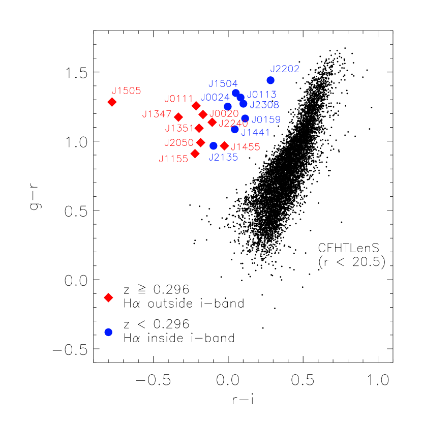
Figure 1: Gemini/GMOS broad-band colours of GBs compared with bright galaxies from the 158 square degrees of CFHTLenS.

The GB sample is fairly complete over the SDSS-DR8 footprint and the $z=0.12-0.36$ redshift range, with three caveats. First, some SDSS data have lower quality leading to an excess of “green” artefacts, seemingly related to poor seeing. Any GBs in these unusable survey areas were missed. This does not bias the sample as it is simply a matter of slightly lower sky coverage. Second, due to our lower size threshold, smaller GBs might not be recovered from some areas due to seeing variations. Most likely there is a smooth transition between large GPs and small GBs. We are not concerned by this incompleteness as we are interested in the most extended sources, only. Third, if an EELR coincides with a luminous elliptical galaxy ($M_{i}\gtrsim-23$ mag), then the [O iii] EW might not be high enough to distinguish the object and it would be overlooked (see also Section 7.2.5). Lastly, we mention that our search entirely misses low-z LABs that do not emit in [O iii] (should they exist at $z\sim 0.3$). This, however, does not count against the completeness of our initial goal of identifying strong [O iii] emitters.

Not all GBs have been discovered yet as SDSS covers a third of the sky, only. We expect $20-30$ more GBs that are still awaiting their discovery at southern declinations.

2.1.3 Previous discoveries of Green Bean galaxies

GBs have a surface density of $1.1\times 10^{-3}$ deg^-2, falling off the grid of smaller surveys and random observations. There are three exceptions, though. First, J2240$-$0927 ($z=0.326$) was a chance discovery in a CFHT wide-field data set (program ID: 2008BO01; Schirmer et al., 2011). Only because of this coincidence did we learn about the existence of GBs and initiate our survey. Second, J0113+0106 ($z=0.281$) was selected automatically for SDSS spectroscopic follow-up to construct a flux-limited $u$-band sample (SDSS3 target flags U_EXTRA2 and U_PRIORITY). Third, J1155$-$0147 ($z=0.306$; the brightest and largest GB), was picked up independently by the Quasar Equatorial Survey Team (QUEST; Snyder, 1998; Rengstorf et al., 2004). It is the only GB in the QUEST survey area, a 2.4 deg wide equatorial strip drift scanned for emission line objects. Chandra images were taken in 2003 (PI: Coppi; Chandra Proposal Number 03700891; title: The X-ray Emission Of High Luminosity Emission Line Galaxies: Quasar-2s And The Starburst-AGN Connection). We did not find any publications of these data, nor about J1155$-$0147 itself.

Table 1: General properties of the GBs and their optical data. Column 1 lists the full names, which we abbreviate in the main text to the first four digits in RA and Dec. Columns 2 and 3 contain the decimal sky coordinates. The spectroscopic redshift is given in column 4. Columns 5, 6 and 7 contain the SDSS $r$-band AB magnitude and the $g-r$ and $r-i$ colours, respectively. Column 8 lists the $r$-band image seeing, translated to a physical resolution (at the respective source redshift) in column 9.

Name	$\alpha_{2000.0}$	$\delta_{2000.0}$	z	$r$	$g-r$	$r-i$	Seeing	Resolution
	[deg]	[deg]		[mag]	[mag]	[mag]		[kpc]
SDSS J002016.44$-$053126.6	5.06852	-5.52405	0.334	18.3	$1.19$	$-0.17$	0$.\!\!^{\prime\prime}$59	2.8
SDSS J002434.90$+$325842.7	6.14543	32.97852	0.293	18.2	$1.25$	$-0.00$	0$.\!\!^{\prime\prime}$69	3.0
SDSS J011133.31$+$225359.1	17.88879	22.89976	0.319	19.1	$1.26$	$-0.21$	0$.\!\!^{\prime\prime}$59	2.8
SDSS J011341.11$+$010608.5	18.42129	1.10237	0.281	18.5	$1.32$	$0.08$	0$.\!\!^{\prime\prime}$77	3.3
SDSS J015930.84$+$270302.2	29.87851	27.05062	0.278	18.9	$1.16$	$0.11$	0$.\!\!^{\prime\prime}$57	2.4
SDSS J115544.59$-$014739.9	178.93580	-1.79443	0.306	17.9	$0.91$	$-0.22$	0$.\!\!^{\prime\prime}$70	3.2
SDSS J134709.12$+$545310.9	206.78802	54.88637	0.332	18.7	$1.17$	$-0.33$	0$.\!\!^{\prime\prime}$37	1.8
SDSS J135155.48$+$081608.4	207.98117	8.26900	0.306	19.0	$1.09$	$-0.19$	0$.\!\!^{\prime\prime}$71	3.2
SDSS J144110.95$+$251700.1	220.29561	25.28337	0.192	18.5	$1.09$	$0.04$	0$.\!\!^{\prime\prime}$52	1.7
SDSS J145533.69$+$044643.2	223.89036	4.77866	0.334	18.5	$0.97$	$-0.03$	0$.\!\!^{\prime\prime}$55	2.7
SDSS J150420.68$+$343958.2	226.08615	34.66618	0.294	18.7	$1.35$	$0.05$	0$.\!\!^{\prime\prime}$37	1.6
SDSS J150517.63$+$194444.8	226.32347	19.74578	0.341	17.9	$1.28$	$-0.78$	0$.\!\!^{\prime\prime}$52	2.5
SDSS J205058.08$+$055012.8	312.74198	5.83688	0.301	18.6	$0.99$	$-0.18$	0$.\!\!^{\prime\prime}$77	3.5
SDSS J213542.85$-$031408.8	323.92855	-3.23577	0.246	19.2	$0.97$	$-0.10$	0$.\!\!^{\prime\prime}$72	2.8
SDSS J220216.71$+$230903.1	330.56961	23.15086	0.258	18.9	$1.44$	$0.28$	0$.\!\!^{\prime\prime}$53	2.1
SDSS J224024.11$-$092748.1	340.10044	-9.46335	0.326	18.3	$1.14$	$-0.11$	0$.\!\!^{\prime\prime}$69	3.3
SDSS J230829.37$+$330310.5	347.12239	33.05291	0.284	19.1	$1.27$	$0.10$	0$.\!\!^{\prime\prime}$67	2.9

2.2 Optical imaging with Gemini/GMOS

We obtained $gri$ broad-band imaging of all 17 GBs. J2240$-$0927 was discovered earlier in deep CFHT data (Section 2.1.3). The remaining GBs were observed with GMOS-N and GMOS-S at the 8-m Gemini Telescopes in Hawaii and Chile, respectively (program IDs GS-2013A-Q-48, GN-2014B-Q-78, GN-2015A-DD-3, GN-2015A-FT-23). $20$ minutes exposure time per filter were sufficient as the targets are bright ($r\sim 18$ mag). The GMOS data were obtained in grey time, under clear and thin cirrus conditions with good seeing.

Several of our targets were re-observed in $griz$ bands at the 4-m Southern Astrophysical Research Telescope (SOAR, Chile) during the science verification runs of the SOAR Adaptive Module (SAM) and the SAM Imager (SAMI; Tokovinin et al., 2010; Tokovinin et al., 2012). SAMI has a 3$.\!\!^{\prime}$1 field of view. SAM corrects for ground layer turbulence using three natural guide stars and one UV laser guide star, achieving a homogeneous PSF across the field and at optical wavelengths. Unfortunately, the seeing during these nights was dominated by turbulence in the upper atmosphere and SAM’s ground layer correction could not yield an improvement over the GMOS data. The only exception are the $r$-band data of J0113+0106 for which the corrected seeing is 0$.\!\!^{\prime\prime}$62 while the DIMM seeing was stable between 1$.\!\!^{\prime\prime}$0$-$1$.\!\!^{\prime\prime}$1; the GMOS image seeing for this object is 0$.\!\!^{\prime\prime}$80. We use the SAMI images to characterize the morphology of J0113+0106.

Image processing was done with THELI (Schirmer, 2013; Erben et al., 2005) using standard procedures. Photometric zeropoints were tied to SDSS field magnitudes, correcting for non-photometric conditions. The physical resolution of the coadded images is between $1.6-3.5$ kpc, depending on seeing and source redshift. Table 1 summarizes the optical characteristics. The fully calibrated, coadded $gri$ FITS images are publicly available.

2.3 Optical spectroscopy with Gemini/GMOS

We conducted a sparse redshift survey around 13 GBs to study their environment, using GMOS poor weather programs (GN-2015A-Q-99, GS-2015A-Q-99; thin cirrus, seeing $\gtrsim$1$.\!\!^{\prime\prime}$2, bright moon). We used the 1$.\!\!^{\prime\prime}$5 long-slit with the B600 grating, tuning the central wavelength to the 4000 Å break at the GBs’ redshifts. Main redshift indicators are Ca h+k, [O ii], [O iii] and the Balmer series. $3\times 600$ s exposures were used with $4\times 4$ detector binning. Target selection was heterogeneous and incomplete. We aimed at galaxies whose angular diameters, magnitudes and colours suggest similar redshifts as the GBs. Red sequence galaxies were preferred if present. High priority was given to galaxies in the immediate vicinity of the GBs, in particular if merger signatures such as tidal tails, extended haloes, and warps are visible. Position angles were chosen to maximize the number of objects (up to 7) on the slit. Up to three slit positions were observed per target area, and a total of 52 redshifts were obtained. Results are presented in Section 5.1 and Table 5.

2.4 Optical spectroscopy with Lick/Kast

Four of the GBs from S13 were observed with the Kast double-beam spectrograph at the 3-m Shane telescope of Lick Observatory to determine their redshifts. A dichroic beamsplitter divided the beams at 4600 Å. The blue arm used a grism setting spanning the $3390-4720$ Å range with a dispersion of 0.65 Å pixel^-1 and a resolution of 3.3 Å FWHM. The red spectra covered $5010-7840$ Å at 2.4 Å pixel^-1 and resolution of 6.1 Å FWHM. The $2^{\prime\prime}$ slit was oriented on a position angle chosen for each object to maximize the line flux included (and the angular span for any kinematic information).

Individual 30-minute exposures were obtained on 12 and 13 March 2013 UT. Reduction used the IRAF long-slit tasks. A flux calibration was provided by observation of the standard stars G191B2B and BD +26 2606 with the same grism and grating settings each night.

Two of the targets, J1347+5453 ($z=0.332$) and J1504+3439 ($z=0.294$), belong to the sample studied in this paper because (1) their redshifted [O iii] line falls into the $r$-band, and (2) with log([O iii]/H$\beta$)=1.00 and 0.94 they are also highly ionized as all other GBs. The other two, J1721+6322 and J1913+6211, are also highly ionized, yet their redshifts of $z=0.544$ and $z=0.552$ are above our upper redshift cut-off.

2.5 Chandra X-ray imaging of 9 GBs

We selected 9 GBs for follow-up with Chandra, adding to the archival data of J1155$-$0147. The target sample is comprised of GBs with different morphology, [O iii] line structure, and [O iii] vs. mid-IR excess. The latter criterion was chosen to include AGN at different stages of the fading process.

We used the aim point on ACIS/S3 for greater soft response and spectral resolution. As our sources are faint we used the VFAINT mode, and pileup is well below 1 per cent according to PIMMS. The full emission region of each galaxy fit on the single CCD, and on-chip background measurements were sufficient. No other bright X-ray sources are present in the fields. The setup for the archival observations of J1155$-$0147 was similar.

Table 2: MIR and X-ray properties. We list the names in columns 1, the X-ray fluxes, count rates and fractional difference hardness ratios ($HR$) in columns $2-4$. Columns 5 and 6 contain the exposure time and Chandra dataset IDs, respectively.

Name	$F_{22\mu{\rm m}}$	$F_{0.3-8\,{\rm keV}}^{X}$	$R_{\rm obs}$	$HR$	$T_{\rm exp}^{\rm Chandra}$	Chandra
	[mJy]	[erg s-1 cm-2]	[s-1]		[ks]	dataset ID
SDSS J002016.44$-$053126.6	11.7	$2.43\times 10^{-14}$	$2.57\times 10^{-3}$	$0.137\pm 0.015$	30	16100
SDSS J002434.90$+$325842.7	25.4	$1.19\times 10^{-14}$	$1.25\times 10^{-3}$	$-0.083\pm 0.040$	20	16101
SDSS J011133.31$+$225359.1	23.1	$-$	$-$	$-$	$-$	$-$
SDSS J011341.11$+$010608.5	39.7	$8.29\times 10^{-14}$	$8.98\times 10^{-3}$	$0.715\pm 0.010$	15	16102
SDSS J015930.84$+$270302.2	18.1	$1.95\times 10^{-15}$	$2.20\times 10^{-4}$	low	30	16107
SDSS J115544.59$-$014739.9	16.9	$1.18\times 10^{-13}$	$2.01\times 10^{-2}$	$0.351\pm 0.002$	30	3140
SDSS J134709.12$+$545310.9	5.3	$-$	$-$	$-$	$-$	$-$
SDSS J135155.48$+$081608.4	25.7	$-$	$-$	$-$	$-$	$-$
SDSS J144110.95$+$251700.1	19.6	$1.75\times 10^{-14}$	$1.83\times 10^{-3}$	$0.082\pm 0.019$	30	16108
SDSS J145533.69$+$044643.2	20.4	$7.51\times 10^{-15}$	$7.95\times 10^{-4}$	$-0.866\pm 0.088$	20	16103
SDSS J150420.68$+$343958.2	7.6	$-$	$-$	$-$	$-$	$-$
SDSS J150517.63$+$194444.8	49.9	$3.62\times 10^{-14}$	$3.86\times 10^{-3}$	$0.316\pm 0.020$	15	16104
SDSS J205058.08$+$055012.8	49.5	$4.70\times 10^{-14}$	$5.00\times 10^{-3}$	$0.719\pm 0.016$	15	16106
SDSS J213542.85$-$031408.8	3.2	$-$	$-$	$-$	$-$	$-$
SDSS J220216.71$+$230903.1	24.8	$-$	$-$	$-$	$-$	$-$
SDSS J224024.11$-$092748.1	37.4	$9.76\times 10^{-15}$	$1.04\times 10^{-3}$	$-0.077\pm 0.067$	15	16105
SDSS J230829.37$+$330310.5	13.9	$-$	$-$	$-$	$-$	$-$

Count rates were estimated with the AGN MIR X-ray correlation of Ichikawa et al. (2012) using SWIFT/BAT and AKARI. By using the hard $14-195$ keV band, Ichikawa et al. (2012) avoid complications by absorption at softer energies. We used their offset between the WISE and AKARI bandpasses, and estimated the GBs’ intrinsic $14-195$ keV luminosities from WISE 22 $\mu$m data. We then inferred the Chandra/ACIS-S $0.3-8$ keV count rate using PIMMS, assuming a power law with photon index $\Gamma=1.9$ for the unabsorbed AGN spectrum, and a column density of $N_{\rm H}=10^{23}$ cm^-2. Our choices for $\Gamma$ and $N_{\rm H}$ were based on our analysis of the J1155$-$0147 data (Section A.6.1).

We chose Chandra/ACIS exposure times of $15-30$ ks, aiming at a total of $\sim 1000$ counts per target. This would secure a successful spectral analysis for the entire sample. In the limiting case of Compton thick absorption ($N_{\rm H}=1.5\times 10^{24}$ cm^-2), without reflection the continuum count rate would be $\sim 0.002$ s^-1. In these instances we would still detect an absorbed AGN in the strong Fe K$\alpha$ line. Note that even a low column density of $N_{\rm H}=10^{22}$ cm^-2  is sufficient to account for the non-detection of all targets by ROSAT (which is sensitive at soft energies only).

Observations were carried out in Chandra cycle 15, and the event files were processed in CIAO following standard procedures. We corrected the WCS of the final X-ray maps by about half a Chandra pixel. The offset was calculated from the mean displacement observed between other X-ray detected AGN in the field and their counterparts in the optical GMOS images. The GBs were excluded from this calculation to avoid biasing by any true offset of their AGN with respect to the peak of the optical emission. Our X-ray measurements are summarized in Table 2.

Figure 2: The GALEX FUV effective area, reproduced from the GALEX online documentation. The GBs’ redshifted Ly $\alpha$ wavelengths fall into the region of highest sensitivity.

2.6 GALEX observations

GALEX data are perfectly suited to detect redshifted Ly $\alpha$ from the GBs in the FUV channel ($1340-1800$ Å; Fig. 2). In the course of the various GALEX surveys, 5 GBs were observed in the FUV with exposure times of $1200-2800$ s, and 10 GBs with exposure times of $60-300$ s. Spectroscopic data were not taken. 14 out of 15 GBs are detected in the FUV, with ${\rm S/N}=2-21$. For two GBs no FUV data are available, but they are visible in the NUV ($1750-2800$ Å). Only J0111+2253 is not detected in the FUV nor the NUV.

Flux measurements were taken from the GALEX DR6 catalogue query page. If multiple measurements of the same source were available, then we used the one with the longest exposure time. The only exception is J1455$+$0446, which is marginally blended in the GALEX data with a large foreground galaxy and not available as a separate catalogue entry. We downloaded the calibrated FUV and NUV images and measured the fluxes in a 10$.\!\!^{\prime\prime}$5 wide circular aperture, cleanly separating J1455$+$0446 from its neighbour. The background signal and measurement errors were estimated by placing the same aperture at 10 randomly chosen nearby blank positions. The FUV and NUV spectral flux densities, exposure times, galactic reddening and estimated Ly $\alpha$ luminosities are listed in Table 3.

3 Analysis of the X-ray data

3.1 Absence of kpc-scale AGN binaries

Many GBs are interacting and/or merging (Sects. 5.2 and 5.3), and could perhaps host binary AGN. Mergers boost the accretion rates of supermassive black holes (SMBHs) by funnelling more gas toward the centres. This also holds for binary AGN as shown by Liu et al. (2012), who find that the log([O iii]) luminosity increases by $0.7\pm 0.1$ in AGN binaries when their separation decreases from 100 to 5 kpc. Therefore, the GBs’ high [O iii] luminosities make binary AGN at least plausible. The fraction of binaries with separations of tens of kpc amongst optically selected AGN is small (3.6 per cent; Liu et al., 2011), yet it could be enhanced in GBs. The GBs’ complex line profiles S13, Davies et al., 2015, though, are much more likely caused by gas kinematics (e.g. Shen et al., 2011; Comerford et al., 2012; Comerford & Greene, 2014; Allen et al., 2015).

We find that the nuclei in GBs are X-ray point sources. If binary AGN are present, then their separations must be smaller than $1.7-1.9$ kpc (about one Chandra ACIS pixel), and/or the secondary AGN is below our detection limit. Nonetheless, the advanced merger states make it worthwhile to search for sub-kpc binaries at other wavelengths.

3.2 Offsets between X-ray and [OIII] peaks

The positions of the X-ray peaks are fully consistent with the positions of the optical peaks in the $r$-band images, i.e. the location of highest [O iii] brightness. The only exception is J1505+1944, where the X-ray peak is offset by 0$.\!\!^{\prime\prime}$5 (2.4 kpc) to the West. Interestingly, the [O iii] nebula in J1505+1944 fragments in East-West direction. The brightest [O iii] part could be powered by a shock or be part of an outflow. Alternatively, it could harbour a second SMBH that is either deeply buried, or faded from our view recently while its ionizing radiation is still propagating outwards; dynamic data are not yet available for this system.

3.3 Diffuse X-ray emission

The X-ray contours are extended for 60 per cent of the targets (J0024, J0159, J1155, J1455, J1055, J2240). While this is weakly significant for most targets individually (caused by just $1-3$ extra counts), in all cases the extended X-ray flux traces the most luminous parts of the [O iii] gas. We think this is caused by photoionized emission from the gas. For the remaining 40 per cent, any diffuse emission is below our detection threshold.

3.4 Compton-thick or intrinsically weak?

Our observations yielded much lower count rates than anticipated, to the point where spectral fitting became meaningless ($7-80$ total counts). Therefore, we did not obtain power law indices, column densities and model fluxes apart from J1155$-$0147.

Figure 3 shows the MIR X-ray relation of Ichikawa et al. (2012). Based on the observed Chandra $0.3-8.0$ keV count rates and a power law index of $\Gamma=1.9$, we calculate the expected X-ray fluxes for four different intrinsic column densities, ${\rm log}\,(N_{\rm H}\,\rm{cm}^{2})=22.0$, 23.0, 24.0 and 24.3; error bars account for an uncertainty of 0.1 in $\Gamma$. The result can be interpreted in two ways: Either, most GBs are nearly or fully Compton-thick (Section 3.4.1), or they have faded recently and quickly, quicker than the typical response time of the dusty tori’s MIR emission (Section 3.4.2).

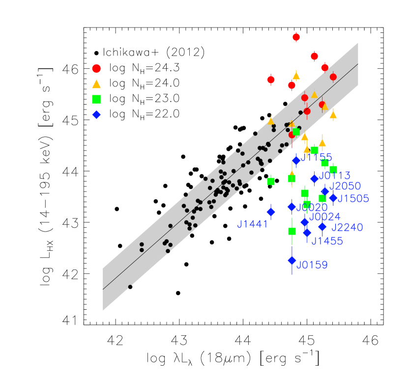
Figure 3: AGN thermal echoes. The black dots show the AGN MIR X-ray relation studied by Ichikawa et al. (2012), the shaded area represents its intrinsic scattering. Overlaid are the expected X-ray luminosities of 10 GBs, based on their observed Chandra $0.3-8.0$ keV fluxes, a power law and 4 different values of intrinsic absorption. Horizontal error bars are smaller than the symbol size, vertical error bars include the Chandra measurement error and a fiducial uncertainty of $\Delta\Gamma=0.1$ for the photon index. The GBs follow the observed MIR X-ray relation only if Compton-thick; since we can exclude Compton-thick obscuration for the sample, the GBs’ X-ray fluxes must have faded quicker than their MIR fluxes, causing thermal echoes. The typical MIR response time-scale to X-ray fading is $10-1000$ years.

3.4.1 GBs cannot be Compton-thick as a sample

The low count rates could be explained if, on average, GBs are obscured with log$\,(N_{\rm H}\,\rm{cm}^{2})=24.1$, implying a Compton-thick fraction $f_{\rm CTK}\sim 0.9$. The latter is unusually high; for comparison, Risaliti et al. (1999), Guainazzi et al. (2005) and Malizia et al. (2009) find $f_{\rm CTK}=0.4-0.5$ for optically and X-ray selected Seyfert-2s at $z\leq 0.035$, and Bassani et al. (1999) report $f_{\rm CTK}=0.23-0.30$.

It is well-known that the fraction of absorbed AGN with log$\,(N_{\rm H}\,\rm{cm}^{2})>22$ decreases with increasing X-ray luminosity (Hasinger, 2008; Ueda et al., 2014; Merloni et al., 2014). How luminous are the AGN in GBs, and what fraction of Compton-thick sources should we expect? Compared to the type-2 samples of Reyes et al. (2008) and Mullaney et al. (2013), GBs rank amongst the most [O iii] luminous type-2 AGN known, and should harbour AGN of high bolometric luminosity (Bassani et al., 1999; Heckman et al., 2004; Lamastra et al., 2009). For e.g. J2240$-$0927, S13 measure an extinction corrected $L_{[\textup{O\,{iii}}]}=(5.7\pm 0.9)\times 10^{43}$ erg s^-1, translating to $L_{\rm bol}\sim 2.3\times 10^{46}$ erg s^-1  following Lamastra et al. (2009). We should therefore expect low values for $f_{\rm CTK}$.

Just how low can be estimated from Ueda et al. (2014) and their fig. 13, showing the fractions of moderately absorbed AGN (log$\,(N_{\rm H}\,\rm{cm}^{2})=22-24$) and Compton-thick AGN (log$\,(N_{\rm H}\,\rm{cm}^{2})=24-26$). Amongst type-2 AGN, $f_{\rm CTK}=0.3$ and 0.05 for the lower and higher X-ray luminous sources, respectively. Both values are in strong disagreement with $f_{\rm CTK}=0.9$ for the GBs.

However, these statistical arguments alone are insufficient to reject the hypothesis that nearly all GBs are Compton-thick. After all, GBs were discovered only recently and have not been studied before. The selection function of GBs (essentially, $r$-band excess caused by [O iii]) favours the selection of optically absorbed AGN: if unabsorbed type-1 AGN were present amongst the GBs, then their continuum contribution to the broad-band photometry would reduce the $r$-band excess and they would not be selected. Therefore, some obscuration amongst GBs is expected, but they do not have to be exclusively Compton-thick.

3.4.2 GBs are intrinsically X-ray weak

If GBs were indeed Compton-thick, then we would still detect the fluorescent K$\alpha$ line (Krolik & Kallman, 1987). However, this line is largely absent in our sample, favouring intrinsically weak AGN over heavy obscuration. The only GB for which we detect K$\alpha$ is J1155$-$0147, which is sufficiently bright to allow for spectral modelling. This is a moderately obscured source (Section A.6.1).

Another indicator for intrinsically weak AGN comes from the fractional difference hardness ratio,

$$HR=\frac{H-S}{H+S}\;.$$ (3)

Here, $S$ and $H$ are the counts in the soft ($0.3-2.0$ keV) and hard ($2.0-8.0$ keV) bands, respectively. We observe a moderate sample mean of $\langle HR\,\rangle=0.14\pm 0.48$ (Table 2), meaning that the AGN cannot be deeply buried as a group.

Table 3: UV properties of the GBs, including the observed monochromatic FUV and NUV spectral flux densities (uncorrected for galactic extinction), the colour excess for the respective line of sight, an extinction-corrected estimate of the Ly $\alpha$ luminosity assuming no continuum, and the GALEX integration times. See text for details.

Name	$f_{\nu}^{\;\rm FUV}$	$f_{\nu}^{\;\rm NUV}$	$E(B-V)$	$L_{\rm Ly\alpha}$	$T_{\rm exp}^{\;\rm FUV}$	$T_{\rm exp}^{\;\rm NUV}$
	[$\mu$Jy]	[$\mu$Jy]	[mag]	[$10^{43}$ erg s-1]	[s]	[s]
SDSS J002016.44$-$053126.6	$9.5\pm 2.3$	$9.0\pm 2.4$	0.030	$2.42\pm 0.59$	206	206
SDSS J002434.90$+$325842.7	$5.9\pm 2.2$	$15.1\pm 1.8$	0.051	$1.12\pm 0.42$	247	501
SDSS J011133.31$+$225359.1	undetected	undetected	0.034	$\lesssim 0.31$	110	110
SDSS J011341.11$+$010608.5	$15.86\pm 0.50$	$15.44\pm 0.50$	0.028	$2.29\pm 0.07$	2743	7999
SDSS J015930.84$+$270302.2	$7.1\pm 2.4$	$9.9\pm 2.2$	0.056	$1.23\pm 0.42$	186	186
SDSS J115544.59$-$014739.9	$40.8\pm 1.9$	$41.2\pm 1.1$	0.019	$6.64\pm 0.31$	2768	2768
SDSS J134709.12$+$545310.9	$31.0\pm 5.3$	$14.3\pm 2.4$	0.010	$6.47\pm 1.11$	190	190
SDSS J135155.48$+$081608.4	$18.1\pm 5.2$	$7.6\pm 2.5$	0.020	$2.97\pm 0.86$	106	106
SDSS J144110.95$+$251700.1	$29.5\pm 8.5$	$16.6\pm 0.9$	0.023	$1.29\pm 0.37$	61	1690
SDSS J145533.69$+$044643.2	$19.8\pm 1.6$	$7.4\pm 1.5$	0.033	$5.14\pm 0.42$	1650	1650
SDSS J150420.68$+$343958.2	$2.7\pm 1.1$	$10.1\pm 0.8$	0.012	$0.38\pm 0.16$	306	2275
SDSS J150517.63$+$194444.8	$22.7\pm 3.5$	$25.4\pm 2.6$	0.033	$6.84\pm 1.06$	234	234
SDSS J205058.08$+$055012.8	$6.6\pm 2.5$	$12.2\pm 1.3$	0.088	$1.77\pm 0.68$	169	1616
SDSS J213542.85$-$031408.8	$18.0\pm 1.3$	$15.9\pm 1.3$	0.033	$1.58\pm 0.11$	1561	1561
SDSS J220216.71$+$230903.1	no data	$11.4\pm 2.8$	0.072	$-$	$-$	173
SDSS J224024.11$-$092748.1	$21.2\pm 1.6$	$14.3\pm 1.0$	0.052	$5.43\pm 0.41$	1578	1578
SDSS J230829.37$+$330310.5	no data	$5.7\pm 2.5$	0.073	$-$	$-$	158

4 Analysis of the GALEX data

In this Section we estimate the Ly $\alpha$ luminosities of the GBs using GALEX FUV and NUV broad-band imaging data (Table 3). In the absence of GALEX spectra, we must estimate continuum contributions to the FUV, which could be mistaken for Ly $\alpha$ emission. We do not have sufficient ancillary data available to perform this for all GBs in our sample. Nonetheless, in four cases we can do this, and we show that continuum emission contributes at most a few 10 per cent to the FUV flux. As the properties of the GBs are similar, we argue that our conclusions hold for the sample as a whole.

If the continuum contribution was 25 per cent, then 85 per cent (53 per cent) of the GBs have Ly $\alpha$ luminosities in excess of $1\times 10^{43}$ ($2\times 10^{43}$) erg s^-1 with Ly $\alpha$ EWs of up to $1000$ Å. We conclude that we have indeed found LABs at low redshift, 17 years after their initial discovery at high redshift (see also Fig. 5).

4.1 Estimating the Ly $\alpha$ luminosities

We correct the FUV spectral flux densities for galactic extinction using the Schlafly & Finkbeiner (2011) tables and a $R_{v}=3.1$ dust model. The correction factors range between 1.08 (J1347+5453) and 1.97 (J2050+0550), and are calculated for the redshifted Ly $\alpha$ wavelengths assuming that most of the FUV flux is caused by this line. Other bright lines such as CIV$\lambda$1549 are redshifted beyond the GALEX FUV bandpass even for the lowest redshift in our sample ($z=0.192$, J1441+2517).

We must account for the relative response function of GALEX when estimating the total Ly $\alpha$ flux from the FUV broad-band data. The bandpass-averaged observed monochromatic spectral flux density, $f_{\nu}^{\;\rm obs}$, is calculated from the redshifted source spectrum, $f_{\nu}(\nu)$, as

$$f_{\nu}^{\;\rm obs}=\frac{\int{f_{\nu}(\nu)\,T(\nu)\,{\rm d}\nu}}{\int{T(\nu)\,{\rm d}\nu}}\;.$$ (4)

Here, $T(\nu)$ is the unnormalized relative system throughput which we interpolate from the FUV effective area (Fig. 2).

We approximate the spectrum as the sum of a constant continuum and some line profile. The continuum is parametrized as a fraction $c$ of the observed spectral flux density, $f_{\nu}^{\;\rm obs}$, and the spectrum is written as

$$f_{\nu}(\nu)=c\,f_{\nu}^{\;\rm obs}\,+\,f_{\nu}^{\;\rm line}(\nu)\,.$$ (5)

Insert this into equation (4) and we have

$$(1-c)\,f_{\nu}^{\;\rm obs}=\frac{\int{f_{\nu}^{\;\rm line}(\nu)\,T(\nu)\,{\rm d}\nu}}{\int{T(\nu)\,{\rm d}\nu}}\;.$$ (6)

The Ly $\alpha$ line width is just a few Å even for a velocity dispersion of 1000 km s^-1. The GALEX FUV response can be considered constant over such small a wavelength range. We model the line profile as a Dirac delta function, normalized to yield the total line flux density, $F_{{\rm Ly}\alpha}$, when integrated over frequency:

$$(1-c)\,f_{\nu}^{\;\rm obs}=\frac{\int{F_{{\rm Ly}\alpha}\;\delta_{\rm D}(\nu-\nu_{{\rm Ly}\alpha})\,T(\nu)\,{\rm d}\nu}}{\int{T(\nu)\,{\rm d}\nu}}=F_{{\rm Ly}\alpha}\;\frac{T(\nu_{{\rm Ly}\alpha})}{\int{T(\nu)\,{\rm d}\nu}}\;.$$ (7)

Here, $\nu_{{\rm Ly}\alpha}$ is the frequency of the redshifted Ly $\alpha$ line. We solve for $F_{{\rm Ly}\alpha}$ and derive the Ly $\alpha$ luminosity using the luminosity distance. In Table 3 we list the Ly $\alpha$ luminosities assuming no continuum ($c=0$). If a fraction $c$ of the FUV flux is in the continuum, then the true line flux will be $(1-c)$ times the tabulated value.

Possible continuum sources are stars, the nebular continuum, and scattered AGN light:

$$c=c^{\,\rm stellar}+c^{\,\rm nebular}+c^{\,\rm scatter}\,.$$ (8)

We discuss each of these terms below.

4.2 Young and old stars must be considered

Young hot stars contribute to the UV continuum. GBs are gas rich and often found in mergers (Section 5.2), a combination known to boost star formation. AGN feedback may also trigger star formation by shock-inducing cloud collapse (e.g. Silk et al., 2013; Silk, 2013). However, our images also bear evidence for strong AGN-driven outflows, which may quench star formation by removing gas (e.g. DeGraf et al., 2014). High values of log([O iii]/H $\beta)\sim 1$ show that star formation plays a minor role at least for the optical line emission (S13).

Old stars with high surface temperatures also contribute to the UV continuum. This includes binary stars (Han et al., 2007), low-mass helium-burning stars in the horizontal branch (e.g. Chung et al., 2011; Ree et al., 2012) and evolved post-AGB stars (e.g. Conroy & Gunn, 2010). These types are thought to cause the UV excess (UVX) observed in elliptical galaxies, in particular bluewards of 2000 Å (UV upturn; for a review see O’Connell, 1999).

Which stellar populations are present in GBs? The red colours of the host galaxies (e.g. J1347+5453, J1504+3439) and of tidal stellar debris (J0024+3258, J0111+2253) are consistent with the prevalence of older stars. In most other cases the host galaxies are too compact to determine reliable colours in the presence of the nebular emission. Four GBs (J1155$-$0147, J1505+1944, J2050+0550, J2202+2309) are in groups or clusters with masses of at most a few $10^{13}\;M_{\odot}$ (e.g. Section A.6). Dynamical friction (Chandrasekhar, 1943; Nusser & Sheth, 1999) and merging is efficient in such low velocity environments, as witnessed by the presence of red sequence galaxies. It is plausible that these four GBs are also red sequence galaxies as they share the same environment with their neighbours.

We have to assume that both young and old stars contribute to the FUV continuum. We can estimate this for J2240$-$0927, for which we have useful spectra (Section 4.3), and for three other GBs where sufficient red sequence galaxies and GALEX data are available (Section 4.4).

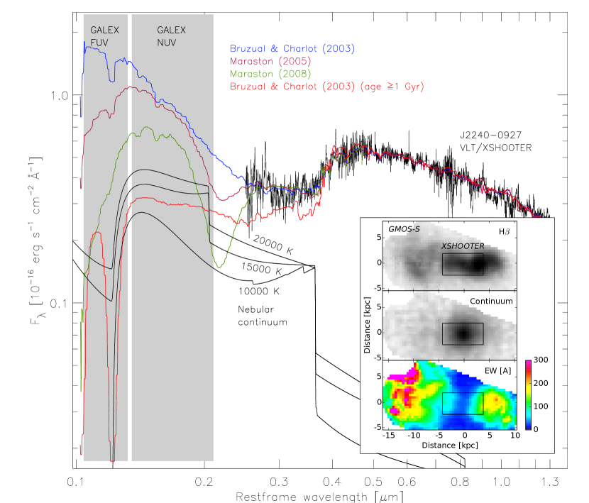
Figure 4: Continuum restframe VLT/XSHOOTER spectrum of J2240$-$0927 (black, emission lines and nebular continuum removed). Overplotted are three representative composite SSP models, used to predict the luminosities in the (blueshifted) GALEX FUV and NUV bandpasses (shaded areas). Comparison with an old stellar base population (red line) reveals excess flux below 3800 Å, requiring additional young stars. The SSP models are divergent below 2500 Å for which we do not have observational data. Also shown is the nebular continuum for three electron temperatures and $n_{\rm e}=100$ cm^-3. The XSHOOTER spectrum was centred on the nucleus, and the extraction area is shown in the lower right inset. The latter displays the reconstructed 2D images (nonlinear stretch) from the GMOS-S data cube, near and on the H$\beta$ line, and the H$\beta$ equivalent width.

4.3 Constraining the stellar FUV/NUV flux for J2240$-$0927 using SED fitting

Davies et al. (2015) have presented a 3D spectroscopic study of J2240$-$0927. The continuum maps reveal a compact spherical galaxy with $\lesssim 9$ kpc diameter. Our VLT/XSHOOTER spectrum (S13) of the nucleus covers the $2500-18800$ Å restframe range. It is corrected for galactic extinction using a $R_{V}=3.1$ dust model and the extinction maps of Schlafly & Finkbeiner (2011), de-redshifted, and we subtract the nebular continuum for a 15000 K hydrogen helium gas mix in ionization equilibrium (see also Section 4.5). We then fit a combination of simple stellar populations (SSPs) with the STARLIGHT code (Mateus et al., 2006), and determine the FUV and NUV fluxes permitted by the models.

We use the evolutionary models of Bruzual & Charlot (2003), the SSPs of Maraston (2005), which include the effects of thermally pulsating AGB stars (TP-AGB), Maraston et al. (2009), the binary SSPs of Han et al. (2007), and lastly the SSPs of Conroy & Gunn (2010), which better describe the UV properties of the horizontal branch and post-AGB stars. A comparison can be found in Conroy & Gunn (2010).

We run STARLIGHT on a grid with 90 different configurations (SSPs, dust and extinction models, hard and soft convergence criteria, wavelength ranges). Figure 4 shows the spectrum together with a choice of three composite SSP models, displaying the full range of predicted FUV/NUV fluxes including extreme cases. We summarize our findings:

First, none of the fits is superior. The continuum levels and slopes are reproduced by all fits for $\lambda\gtrsim 2800$ Å, whereas absorption features (CaH+K, G-band, Mg, NaD, Ca ii triplet, etc) are recovered with lesser accuracy. Inclusion of different dust models and extinction laws do not change the fits significantly.

Second, we observe absorption bands near 8500 Å and 9500 Å, attributed to TP-AGB stars, CN and CO bands, and they are better described by the MA05 models. All fits reproduce the spectrum well between $13000-19000$ Å (not shown in Fig. 4).

Third, a reference model consisting of old populations with ages $\geq 1$ Gyr only (red line), reveals excess flux below 3800 Å. Consequently, all models require the presence of a younger population with age of a few to a few ten Myrs. Depending on the STARLIGHT setup, $10-30$ per cent of the bolometric luminosity are caused by young stars. This contribution drops to 2 per cent when we exclude wavelengths shorter than 3800 Å from the fit.

Fourth, all models diverge below 2500 Å. This is caused by the strong metallicity and age dependence of the UV upturn which is unconstrained by our data.

Finally, we shift the various composite SEDs to the redshift of J2240$-$0927, add back the reddening, and calculate bandpass-averaged FUV/NUV spectral flux densities for comparison with the GALEX data. We apply aperture correction factors, as GALEX integrated the entire galaxy light, whereas XSHOOTER observed through a 0$.\!\!^{\prime\prime}$9 wide slit. To this end we use the 3D GMOS-S spectroscopic cube of Davies et al. (2015), which covers the full spatial extent of J2240$-$0927. We integrate the light over the reconstructed IFU image, once over the full field, and once within the XSHOOTER aperture. Seeing corrections are unnecessary because both data sets were taken with a seeing of 0$.\!\!^{\prime\prime}$5$-$0$.\!\!^{\prime\prime}$6. For the stellar continuum (taken near H$\beta$) and the nebular emission (taken on H$\beta$) we determine aperture correction factors of $2.10\pm 0.04$ and $2.65\pm 0.05$, respectively. The nebular correction factor is larger because the continuum light is much more concentrated (see the inset in Fig. 4).

4.3.1 Results of the SED fitting

The observed GALEX FUV flux density of J2240$-$0927 is $21.2\pm 1.6$ $\mu$Jy (Table 3). We find the stellar model fluxes to range between $2.7-12.1$ $\mu$Jy (most extreme values, $13-57$ per cent contribution). Deeper observations below restframe wavelengths of 2500 Å (observed 3400 Å) are required to better discriminate between the models. The flux calibration and S/N of our XSHOOTER observations (${\rm S/N}\sim 1$ after $32\times$ spectral binning) are too poor for this purpose. Given these data alone, the most plausible contribution is $\sim 5-8$ $\mu$Jy, i.e.

$$c^{\,{\rm stellar}}=0.2-0.4\;\;({\rm J2240-0927}).$$ (9)

For the NUV, we find stellar model flux densities between $10.1-16.7$ $\mu$Jy, compared to an observed value of $14.28\pm 0.95$ $\mu$Jy. Consequently, the model that produces the lowest FUV contribution of 13 per cent accounts for 70 per cent of the observed NUV flux, ruling out models that contribute more than about $20$ per cent to the FUV. Including this constraint from the NUV data, we update

$$c^{\,{\rm stellar}}\lesssim 0.1-0.2\;\;({\rm J2240-0927}).$$ (10)

4.4 Constraining the stellar FUV flux in 3 GBs from red sequence galaxies

J1155$-$0147, J1505$+$1944 and J2050$+$0550 are in spectroscopically confirmed galaxy groups with a red sequence. We derive mean stellar FUV to $i$-band flux ratios, $\langle f_{\nu}^{\,\rm FUV}/f_{\nu}^{\,i}\rangle$, for the red sequence members. Assuming that the GBs are also red sequence members, we use their $i$-band magnitude to estimate their stellar FUV flux (note that H $\alpha$ is redshifted beyond $i$-band in all three cases).

We place apertures over the red sequence members in the $i$-band image and measure their $i$-band spectral flux density. The apertures are then transformed to the GALEX FUV image accounting for the larger plate scale and PSF, and the measurement is repeated. The red sequence members are not detected individually by GALEX. Integrating over all apertures, we derive $\langle f_{\nu}^{\,\rm FUV}/f_{\nu}^{\,i}\rangle=(5.0\pm 6.5)\times 10^{-3}$, $(-2.7\pm 2.0)\times 10^{-3}$, and $(1.07\pm 0.62)\times 10^{-2}$, respectively, for these three systems. This describes the total FUV contribution from young and old stars. Comparison with the observed FUV flux densities yields

$$c^{\,{\rm stellar}} = 0.027\pm 0.035\;\;({\rm J1155-0147})$$ (11)

$$c^{\,{\rm stellar}} < 0.018\;\;({\rm J1505+1944;\;95\,\%\;confidence)}$$ (12)

$$c^{\,{\rm stellar}} = 0.11\pm 0.07\;\;({\rm J2050+0550}).$$ (13)

The value for J1505$+$1944 is an upper limit. These contributions are lower than or equal to what we have found for J2240$-$0927 using SED fitting. All GB host galaxies have similar $i$-band magnitudes ($18.8\pm 0.4$ mag). Stars, therefore, cannot explain their high FUV fluxes (accounting for a few per cent, at most a few 10 per cent of the FUV flux).

4.5 Nebular continuum for J2240-0927

The nebular continuum also contributes to the UV. We model it using our custom-made software NEBULAR (Schirmer 2016, submitted), which is publicly available. In particular, we use a mixed hydrogen helium plasma in ionization equilibrium, with a helium abundance (by parts) of 0.1. The continuum of the nebular spectrum is comprised of free-bound recombination emission from H i, He i and He ii, free-free emission from electrons scattering at charged ions, and the two-photon continuum.

The two-photon continuum far exceeds the free-bound emissivity below 2000 Å. It arises in hydrogenic ions from the decay of the 2${}^{2}S$ level to the 1${}^{2}S$ level by simultaneous emission of two photons (a single photon decay is prohibited by the dipole selection rules). The energy of the two photons adds up to the Ly $\alpha$ energy. The two-photon spectrum has a natural upper cut-off at the Ly$\alpha$ frequency, and peaks at half the Ly$\alpha$ frequency when expressed in frequency units. We approximate the two-photon spectrum following Nussbaumer & Schmutz (1984). The 2${}^{2}S$ level is increasingly de-populated by collisions for electron densities $n_{\rm e}>1000$ cm^-3 (Pengelly & Seaton, 1964), reducing the two-photon continuum. This process can be ignored in the low-density gas (Davies et al., 2015) of the GBs.

At optical wavelengths, the nebular continuum is faint and dominated by the stellar continuum. Fotunately, its amplitude is fixed with respect to the intensity of the Balmer lines at a given electron temperature and density. Using NEBULAR, we derive H$\beta$ equivalent widths of 1370, 770 and 650 Å over the nebular continuum, for electron temperatures of 10000, 15000 and 20000 K, respectively (and $n_{\rm e}=100$ cm^-3). Using the total observed H$\beta$ flux from our GMOS-S data cube ($7.5\times 10^{-15}$ erg s^-1), we find the following: In the FUV, the nebular continuum contributes 0.5, 1.6 and 2.1 $\mu$Jy for $T_{\rm e}=10000$, 15000 and 20000 K, respectively, i.e. 2, 8 and 10 per cent of the observed total FUV flux. Davies et al. (2015) have shown that the typical gas temperature in J2240$-$0927 is around 13800 K, and 15500 K if the hotter nuclear region is included as well.

As can be seen in Fig. 4, the (redshifted) nebular continuum peaks in the GALEX NUV channel (mostly because of the strong two-photon spectrum). Consequently, we determine much higher NUV flux densities of 5.4, 9.0 and 10.3 $\mu$Jy for $T_{\rm e}=10000$, 15000 and 20000 K, respectively (38, 63 and 73 per cent of the observed total NUV flux).

4.5.1 Results for the nebular continuum

The nebular continuum contributes $2-10$ per cent to the FUV flux of J2240$-$0927, and $38-73$ per cent of the observed NUV flux. It is much better constrained than the stellar contribution from SED fitting, because the H$\beta$ line is detected with high S/N and the nebular continuum is fixed to the H$\beta$ flux. The stellar FUV/NUV continuum is much more uncertain as it is mostly unconstrained by observational data below 2500Å. For J2240$-$0927, we have

$$c^{\,{\rm nebular}} = 0.02\;\;({\rm T=10000\,K})$$ (14)

$$c^{\,{\rm nebular}} = 0.08\;\;({\rm T=15000\,K})$$ (15)

$$c^{\,{\rm nebular}} = 0.10\;\;({\rm T=20000\,K}).$$ (16)

The most conservative estimates from the nebular continuum and the stellar continuum easily account for the entire GALEX NUV flux. In the FUV, on the other hand, the largest conceivable combination yields about 30 per cent, and the remainder must be attributed to Ly $\alpha$ .

4.6 Scattered AGN light

Another source of UV continuum is light from the AGN accretion disk, scattered in areas that have an unobscured view of the nucleus (see Pogge & De Robertis, 1993; Zakamska et al., 2005, for examples of scattering in the near UV). Without FUV polarization measurements we cannot constrain this effect directly. The absence of scattered broad lines in the shallow optical spectra of S13 indicates that this effect is insignificant for the sample as a whole. We have also shown above for J2240$-$0927 that the stellar and the nebular continuum fully account for the NUV observations, leaving little to no headroom for additional scattered light (Sects. 4.3 and 4.5). Therefore,

$$c^{\,\rm scatter}\approx 0\,.$$ (17)

5 Analysis of the optical data

In this Section we describe global characteristics of the GBs. Notes about individual targets are given in Appendix A.

5.1 Environment

We obtained 52 spectroscopic redshifts (Table 5) of selected field galaxies to determine the local environment of 13 GBs. The selection function is described in Section 2.3.

The majority of the GBs live in low-density areas. 35 per cent are isolated, and for 25 per cent we can currently not say whether they are isolated as well, or have $1-3$ possible companion galaxies. $15-20$ per cent are located in sparse groups with low concentration and perhaps $3-5$ members. The remaining 25 per cent are found in richer groups of galaxies with $M_{200}=(1-6)\times 10^{13}\;M_{\odot}$ and well-defined red sequences (see Table 4 and Appendix A).

This is in stark contrast with LABs at high redshift, which are preferentially found in filaments and clusters. Possibly, at $z=0.3$ the cold accretion streams have been exhausted, and low-z LABs are mostly formed and ionized by AGN. If a GB is located in an apparent group or cluster, then it is found near the centre of the distribution of galaxies. Particularly noteworthy is J1155$-$0147, dominating the group with its size and luminosity. This is the only GB whose morphology could match a cold accretion stream.

5.2 Merger rates

$50-65$ per cent of the GBs interact or merge as evidenced by extended warped stellar haloes, tidal stellar streams and close companions. Some of the companions show tidal distortions (e.g. J2240$-$0927), others appear spherically compact, undisturbed and just embedded in the gas (e.g. J0020$-$0531). Only 15 per cent of the GBs reveal seemingly tidally undisturbed host galaxies (J0159+2703, J1347+5453, J1504+3439; it is possible that some signs of tidal tails and interactions have been missed due to their low surface brightness). In all other cases, the bright EELR prevents a clear view of the hosts, or the hosts are obviously interacting with their companions. Yajima et al. (2013) have shown with hydrodynamical simulations and radiative transfer calculations that binary galaxy mergers will produce LABs with Ly $\alpha$ luminosities of $10^{42-44}$ erg s^-1  and typical sizes of $10-50$ kpc (like GBs), albeit at $z=3-7$. The Ly $\alpha$ emission in these model mergers is mostly produced by intense star formation and gravitational cooling, whereas in GBs the main power sources are AGN. This is a another indication of a strong redshift evolution of LABs. We discuss this in Section 6.

5.3 Morphologies of the host galaxies

The host galaxies of five GBs are easy to classify because of the EELRs’ low EWs and the hosts’ large diameters. In J0159+2703 we find a large, 46 kpc face-on barred spiral galaxy. J1347+5453 is an edge-on disk with 21 kpc diameter and an axis-ratio of at least 5:1 (the minor axis is not spatially resolved). The $i$-band data reveal a bright bulge or unresolved nucleus. J1504+3439 is an elliptical galaxy with a major axis of 37 kpc. J2202+2309 is a luminous elliptical near the centre of a galaxy cluster. It can be traced over at least $40\times 25$ kpc and is embedded in a common halo with two other ellipticals of similar size and luminosity. The system could form the future brightest cluster galaxy (BCG) of this structure. J2308+3303 is comprised of a 6 kpc bright nucleus surrounded by a face-on featureless disk with $22\times 20$ kpc diameter.

The classification of most other hosts is hampered by the low spatial resolution and strong line emission in the $gri$ filters. They appear to be compact with major axes of $8-18$ kpc (Table 4). Colours of tidal stellar streams suggest older stellar populations, but that does not exclude ongoing star formation. Perhaps the most bizarre object is J1455+0446, consisting of a 40 kpc large jumbled mix of ionized gas and stars as judged by its large colour variations. The bright nucleus is found at the edge of the system. Continuum images from 3D spectroscopy, and $K$-band images of relatively line-free regions of the spectrum would greatly help the classification.

5.4 Morphologies of the emission line regions

The emission line regions in the GBs extend over several 10 kpc. In the absence of kinematic data, the spatial image resolution of $2-3$ kpc allows for some constraints on the formation of the GBs. Most compelling is the bewildering range of morphologies arising from the combination of various intrinsic shapes and viewing angles.

Hainline et al. (2013) have spectroscopically determined the size of [O iii] narrow-line regions (NLRs) around luminous type-2 quasars, measuring within an $1\times 10^{-15}$ erg s^-1 cm^-2 arcsec^-2 isophote. They have found typical sizes of $6-8$ kpc, with an upper limit of $10-20$ kpc. We do not have spectroscopic data at hand for a direct comparison with their results; however, within the same $r$-band surface brightness, and along the minor axis, we find typical sizes of $12-25$ kpc. At these radii the flux is dominated by [O iii] emission, not by $r$-band continuum, thus a comparison of our measurements and those of Hainline et al. (2013) are still meaningful. Hainline et al. (2013) have argued that their size limit is caused by the unavailability of gas at larger radii to be ionized. Likely, this is the reason why our sample differs so much: it was selected because of its extreme broad-band colours, caused by very gas-rich systems.

Liu et al. (2013) and Harrison et al. (2014) have also studied the properties of [O iii] NLRs around luminous radio-quiet type-2 quasars. The sizes of the [O iii] nebulae in GBs are consistent or somewhat larger compared to their results; no corrections are made for methodology. Both authors find mostly circular or moderately elliptical, smooth morphologies for the outflows. Irregular morphologies are commonly coupled with radio excess. This is in stark contrast with the nebulae observed in GBs. Most are highly asymmetric, irregular and patchy, apart from J1351+0816 and J2050+0550, which reveal rather smooth spheres. Again, this could be a selection effect: we found 17 objects in SDSS with extreme broad-band photometry, whereas Harrison et al. (2014) chose 16 AGN out of a parent sample of 24000 SDSS AGN. It is entirely possible that some GBs could have ended up in the sample of Harrison et al. (2014); however, as we have mentioned in Section 2.1.2, the SDSS colour space occupied by GBs is too contaminated for automatic source extraction.

For some targets we give simple estimates about the duration of an AGN burst, and/or the time it must have occurred in the past. For simplicity, we assume a single, average outflow velocity of $v=1000$ km s^-1 and an inclination angle of $\theta=90$ degrees, i.e. the outflows are moving perpendicular to the line of sight. Therefore, time estimates must be scaled by $1000\;{\rm km\;s^{-1}}\;v_{\rm obs}^{\;-1}\;{\rm sin}^{-1}\,\theta_{\rm obs}$ to obtain the true values.

5.4.1 AGN driven outflows

$65-75$ per cent of the EELRs have AGN outflow signatures, such as collimated beams or symmetric ejecta in opposite directions (Table 4). The outflows are usually launched by the injection of thermal energy into the surrounding gas during an AGN burst. The heated gas expands and sweeps up (and shocks) colder material along its path. Such outflows have been well studied both observationally as well as theoretically; a detailed account of these efforts is beyond the scope of our work. We compare our findings to the simulations of Gabor & Bournaud (2014), who typically find unipolar outflows with wide opening angles. Accordingly, denser gas on one side of the nucleus may fully stop an outflow and reradiate its energy, while the outflow may escape on the other side through a thinner interstellar medium. One object in our sample, J0111+2253, fits this picture well. It displays a strong unipolar outflow emerging on one side of the nucleus where it is also wide; a weaker second outflow (or ionized material) is seen at a 30 deg angle, and no outflow is found on the opposite side.

However, J0111+2253 appears to be the exception. For example, we observe bipolar outflows in J0024+3258, J0113+0106 and J1347+5453 that are well focused near the geometric centre of the host galaxy or their nuclei. The southern outflow in J0024+3258 even appears collimated over 15 kpc. J1347+5453 is a posterchild bipolar outflow, launched from the nucleus of a spiral galaxy perpendicular to the edge-on disk.

Some of the outflows must have been sustained over a prolonged time because their gas is continuously distributed all the way to the nucleus. Differential velocities in the outflow will enhance this effect. In case of J0024+3258, the burst would have lasted $8-11$ Myr assuming no velocity dispersion within the stream. Such long (and Eddington-limited) accretion phases are also found by Gabor & Bournaud (2014). Higher resolution images are needed to detect discontinuities in that outflow. J0113+0106, on the other hand, appears to have experienced a powerful event $\sim 5$ Myr ago producing two superbubbles $5-8$ kpc in size on either side of the nucleus. The bubbles are $1.5-2$ times larger than the seeing disk and therefore not well resolved. If the observed distances of the gas from the nucleus are caused by differential gas velocities, then this event could have been much shorter than 1 Myr. Ionized material at larger distances shows that this recent burst was preceded by another one, perhaps $20-30$ Myr ago. Recurrent events likely occurred as well in J1347+5453, J1441+2517, and J1504+3439.

Other systems have a more multipolar character with outflows in different directions. This could be caused by variable gas densities near the nucleus which may partially stop an outflow or divide it (as in the northwestern outflow in J1347+5453, and in J0111+2253).

5.4.2 Cloud systems

Another typical feature are single or multiple regions of gas, apparently detached from the nucleus. We refer to them as clouds. This could be tidally stripped gas contributed by gas-rich mergers and now passing through the AGN’s ionization cones (like in Hanny’s Voorwerp, see Lintott et al., 2009; Rampadarath et al., 2010; Keel et al., 2012a). Typically, these clouds have a relatively smooth appearance and a physical size of $5-15$ kpc. Examples are J1441+2517, J1504+3439, J1505+1944, J2050+0550, and most spectacular in J2240$-$0927 (Davies et al., 2015).

Alternatively, the clouds were ejected during one or more previous bursts, and then disconnected from the nucleus and now reside in the galaxies’ haloes. Currently, this disconnection could be happening in J0024+3258, whose northern outflow appears to be still feeding such a cloud, and in J1347+5453, whose southeastern outflow has a similar structure. In both cases the clouds are significantly misaligned with the feeding stream, as if they experienced tidal dragging or other interactions with the intergalactic medium (see also Section 5.4.3).

5.4.3 Warps

Several EELRs show warps and other symmetric and asymmetric deformations that could be caused by various mechanisms. The gas in J0020$-$0531 resembles a spiral with two widely opened arms that become thinner with increasing nuclear distance. This could be differential orbital motion, tidal interaction with two embedded compact ellipticals, or a continuous change in outflow direction. In J0024+3258, J0113+0106, and J1347+5453 it appears that the ejection direction has changed during or between bursts, or that the gas has been shaped by interactions with the surrounding halo and/or a radio jet. GBs are mostly radio quiet or radio weak (S13), and thus jet interaction is unlikely. Radio data from the VLA FIRST survey (White et al., 1997) have insufficient resolution and depth for further investigation.

Alternatively, the warps could be caused by a change in the ionization cone’s opening angle and strength because of intervening or sublimating dust. Spin precession of the SMBH and its accretion disk could also play a role. Typical precession periods of $10^{3-7}$ years fully overlap with the duration of AGN bursts (Section 6.2), and the precession cones’ half opening angles range from $1-70\,^{\circ}$ (see Lu & Zhou, 2005).

5.4.4 Smooth spheres

The EELRs in J1351+0816 and J2050+0550 are featureless spheres in our data (J2050+0550 is accompanied by an ionized cloud, see above). All systems for which we observe outflow signatures are highly structured, suggesting that a different process has formed these spheres. J2050+0550 is in a cluster of galaxies and could be in an advanced merger state, engulfed in gas that is now ionized by the AGN. [O iii] is detected at least to a radius of 20 kpc by our field redshift survey. J1351+0816, on the other hand, is isolated in the field. Our redshift survey detects [O iii] emission out to a radius of at least 48 kpc. Some process must have transported the gas to these distances. Unfortunately, the depth and resolution of our spectral data are insufficient to obtain kinematics and further constraints.

5.4.5 Peculiar systems

Three GBs are set apart from the rest by their distinct nebular morphologies. First, J1455+0446 appears totally disrupted by a merger. Second, J1504+3409 is reminiscent of the Voorwerpjes, ionization echoes found at low redshift (Keel et al., 2012b). It has several ionized clouds and bubbles superimposed on the body of a larger elliptical galaxy, which distinguishes it from the Voorwerpjes (mostly spirals and irregulars).

Third, and most interesting, is J1155$-$0147. This is the brightest and also intrinsically most luminous object in our sample (both in terms of FUV/Ly $\alpha$ and [O iii]). It is also the largest object in terms of area, and second largest in terms of linear diameter (second to J0113+0106). Curiously, it is also located at the geometric centre of a relatively compact group. The ionized nebula is richly substructered, fragmenting into smaller clouds. A detailed description is given in Appendix A. Possibly, J1155$-$0147 has formed by accretion from the intracluster medium, and its Ly $\alpha$ emission is a mix of AGN photoionization and gravitational cooling radiation.

6 Discussion – AGN variability and LABs

The impact of variable AGN on the appearance of LABs has not yet been studied in detail. In Section 6.1 we review the literature, and in Section 6.2 we present theoretical and observational evidence for significant episodic AGN phases. We discuss the effects of AGN variability on the Ly $\alpha$, MIR and optical properties in Sects. 6.3, 6.4, and 6.5, respectively.

6.1 Earlier considerations about variability

AGN variability as an explanation for the ionization deficits in LABs has not been a serious contender in the light of cold accretion, shocks, starbursts, obscured AGN, and resonant scattering. Nonetheless, it has been mentioned early on: Steidel et al. (2000) have emphasized the absence of strong radio and continuum sources in a luminous LAB and noted the possibility of a “dead radio galaxy”, albeit without elaborating the idea further. Later, Keel et al. (2009) have stated in their summary that “Among the proposed explanations for Ly $\alpha$ blobs … [is] photoionization by active nuclei which may be obscured or transient”. The discovery of Hanny’s Voorwerp, the prototypical quasar ionization echo, has been published soon thereafter by Lintott et al. (2009).

Overzier et al. (2013) have found that LABs with $L_{\rm Ly\,\alpha}\gtrsim 5\times 10^{43}$ erg s^-1  almost always harbour a luminous (obscured) quasar. Given that the AGN duty cycle is much shorter than that of cold accretion, they have argued that the high incidence of obscured quasars in these LABs implies a substantial contribution to the ionization of the gas; the latter could still be provided by cold accretion streams. Furthermore, given the discovery of ionization echoes, they have stated that “[…] episodic AGN activity may need to be considered as well when interpreting high-redshift LABs.

6.2 Evidence for AGN flickering

Cosmological simulations require recurrent periods of rapid black hole growth, setting black hole scaling relations and unleashing strong feedback (Sijacki et al., 2015). Simulations resolving the gas dynamics on sub-kpc scales confirm these sharp intermittent bursts of AGN activity, followed by rapid shutdowns, on time-scales of $\sim 10^{5}$ years (Hopkins & Quataert, 2010; Novak et al., 2011; DeGraf et al., 2014). Mergers, disk bar instabilities, and clumpy accretion may boost the quasar-modes further (e.g. Bournaud et al., 2011; Bournaud et al., 2012).

These predictions have been verified observationally by discoveries of ionization echoes at $z=0.05-0.35$ (Schawinski et al., 2010; Keel et al., 2012a, b; Schirmer et al., 2013; Schweizer et al., 2013; Keel et al., 2015). AGN must undergo several $100-1000$ of these duty cycles (“flickering”) to build up their mass (Schawinski et al., 2015). Independent evidence for flickering, albeit on longer time-scales of $\gtrsim 1-10$ Myrs, has been reported by Kirkman & Tytler (2008) and Furlanetto & Lidz (2011) studying the transverse proximity effect in the hydrogen and helium Ly $\alpha$ forest of selected quasars, respectively (see also Khrykin et al., 2016).

6.3 AGN duty cycles and delayed Ly $\alpha$ response

What does AGN flickering mean for LABs? The escape of Ly $\alpha$ photons is delayed because of resonant scattering, and the Ly $\alpha$ flux will lag behind the light curve of the ionizing source. The effect increases with the optical depth $\tau$, in particular if the ionizing source is a central AGN. The mean optical depth at the Ly $\alpha$ line centre is

$$\tau_{0}=\pi^{-1/2}\,1.04\times 10^{7}\,\left(\frac{T}{10^{4}\,{\rm K}}\right)^{-1/2}\,\left(\frac{N_{\rm HI}}{10^{20}\,{\rm cm^{2}}}\right),$$ (18)

(e.g. Neufeld, 1990; Roy et al., 2010), where $N_{\rm HI}$ is the column number density of neutral hydrogen. Accordingly, LABs with typical temperatures of $\sim 10^{4}$ K can have a great range of optical depths, $\tau=10^{2-4}$ (e.g. Dijkstra et al., 2006), or even higher. At much higher temperatures hydrogen is mostly ionized and optically thin to Ly $\alpha$ .

The spatial transfer of resonantly scattered Ly $\alpha$ photons does not follow a pure Brownian random walk because frequency scattering moves photons out of resonance, and therefore they propagate faster. For these purposes the photon frequency is commonly parametrized as $x=(\nu-\nu_{0})/\Delta\nu_{\rm D}$, measuring the frequency deviation from the resonance frequency, $\nu_{0}$, in units of the Doppler broadening, $\Delta\nu_{\rm D}$. The two maxima of the double-peaked Ly $\alpha$ line profile occur at $|x|\gtrsim 2$ (e.g. Roy et al., 2010).

Roy et al. (2010) and Xu et al. (2011) have studied the Ly $\alpha$ response of spherical Damped Ly $\alpha$ haloes (DLAs; constant hydrogen density and temperature) to an ionizing flash of finite duration. The effect of dust on the escape times is negligible (Yang et al., 2011b). We summarize their results, pertinent to our work, as follows:

1. Typical Ly $\alpha$ escape times for $10-100$ kpc DLAs are $10-100$ times longer than in the absence of resonant scattering; the delay scales roughly with $10\,\tau$. The Ly $\alpha$ response is a very damped version of the light curve of the ionizing source, and the Ly $\alpha$ peak brightness might be reached long after the central source has switched off.

2. Photons with $|x|<4$ are effectively trapped in an optically thick halo and stored for a long time, approximately proportional to $\tau$.

3. Photons with $|x|<2$ are thermalised about 10 times sooner than their typical escape time, meaning they have lost all memory about the location, spectrum and time variability of the source.

The analyses of Roy et al. (2010) and Xu et al. (2011) were performed for spherical DLAs with high $\tau\geq 10^{6-7}$. LABs are complex objects as witnessed by their vast range of morphologies, both for our low-z LABs as well as those at high redshift. AGN outflows may clear escape paths for the Ly $\alpha$ photons through the neutral hydrogen, whereas other regions maintain a high optical thickness. Regardless, the typical double peaked Ly $\alpha$ line profiles show that the effects of resonant scattering are ubiquitous and paramount in LABs. Therefore, the three main results listed above still apply. A more differentiated analysis of these effects on LABs is desirable, and will be presented in Malhotra et al. (2016; in prep.).

We conclude that the observed Ly $\alpha$ fluxes effectively decorrelate from typical AGN flickering. LABs with high Ly$\alpha$ luminosities do not require currently powerful AGN. The LABs could simply be gradually releasing stored photons from earlier high states, while the AGN actually is in a low state. Conversely, a previously dormant AGN could experience several duty cycles, stocking up the halo with Ly $\alpha$ photons well before any Ly$\alpha$ manages to escapes. Herenz et al. (2015) report such Ly $\alpha$ deficient radio-quiet quasars, but do not consider variability as an explanation.

To give an order-of-magnitude calculation: Novak et al. (2011) find that AGN spend perhaps 1 per cent of their time in quasar mode. If the storage time of an optically thick LAB is 10 times longer than the typical burst duration of $\sim 10^{5}$ years (Schawinski et al., 2015), then, statistically, in 90 per cent of the cases we would not detect a quasar in X-rays in a randomly selected sample of the most luminous LABs (if the AGN is below our detection threshold while being in the low state). This explains at least some of the non-detections that have been attributed to heavy obscuration (e.g. Geach et al., 2009; Overzier et al., 2013).

6.4 AGN duty cycles and delayed MIR response (thermal echoes)

6.4.1 GBs must have faded recently to violate the MIR X-ray relation

The X-ray data require the GBs to be intrinsically weak, violating the MIR X-ray relation (Fig. 3). For a fixed column density of $N_{\rm H}=10^{23}$ cm^-2 , the GB sample is a factor of $\sim 30$ fainter than expected from the MIR X-ray relation. This discrepancy increases to a factor of $80$ for $N_{\rm H}=10^{22}$ cm^-2.

The violation is naturally explained by rapid fading of the AGN. Information about a change in nuclear luminosity will take $t_{\,\rm lag}=r_{\,\rm sub}/c$ years to reach the dusty torus at its sublimation radius, $r_{\,\rm sub}$. This time lag is between ten to a few hundred years for typical tori, and is the minimum time for the torus to start a response in the MIR. The actual shape of the response, and the time needed by the torus to reach a new thermal equilibrium, depend on the torus’ radial dust distribution. The directly illuminated surfaces at $r_{\rm sub}$ react quickly (Nenkova et al., 2008), whereas shielded and indirectly illuminated parts further in the back are delayed. Hönig & Kishimoto (2011) have analysed the MIR (and NIR) response of various dusty torus configurations to a discrete pulse from the nucleus with $0.5\,t_{\,\rm lag}$ length. They find that compact tori reach their peak brightness quickly, coincident with the arrival time of the end of the pulse at the sublimation radius at $1.5\,t_{\,\rm lag}$. At $2.5\,t_{\,\rm lag}$ the MIR luminosity has already dropped again to 50 per cent of the peak flux. For thick tori the peak brightness will be reached at a much later time, $\gtrsim 10\,t_{\,\rm lag}$, and the full MIR response can easily be delayed by $10^{3}$ years or more (thermal echoes).

The MIR X-ray relation is easily violated by a transient AGN, in particular for “slow” tori. An individual AGN with high MIR luminosity and low or absent X-ray flux is not necessarily deeply obscured; it might just be fading.

We conclude that the GBs, as a group, have faded by several factors $10-100$ and quicker than the response times of their dusty tori; more accurate evaluations of $N_{\rm H}$ require deeper X-ray observations, or observations extending to higher X-ray energies, and have commenced for some GBs already. Depending on the response times, this change occurred over $10-1000$ years. The [O iii] excess with respect to the MIR emission reported in S13 implies another drop in luminosity by a factor of $5-50$ over the light crossing time of the optical EELR ($10^{4-5}$ years). Taking the thermal echoes and ionization echoes together, the AGN in GBs likely faded by $3-4$ orders of magnitude over the last $10^{4-5}$ years.

6.4.2 Strong thermal echoes are underrepresented in the MIR X-ray relation

The MIR X-ray relation is based on observational data, and as such individual geometric properties, anisotropic shielding as well as AGN variability contribute to its intrinsic scatter. The influence of strong variability, however, is small. Hopkins & Quataert (2010) have shown in their sub-kpc simulations that even for active systems with large time-averaged accretion rates, the instantaneous inflow rates are modest most of the time. The black hole mass is typically built up during many short duty cycles with rapid switch on/off times. The AGN thus spend very little time in the transition phases. Novak et al. (2011) show in their 2D simulations that the AGN duty cycles (defined as the fraction of time above a certain Eddington ratio) are short, typically $10^{-3}-10^{-2}$ or less for an Eddington ratio of 0.1. They do not, however, elaborate on the fraction of time the AGN spend on switching from high to low accretion states (when – and shortly thereafter – we would observe them as echoes). Schawinski et al. (2015) use observations of low-z ionization echoes to argue that the time used to switch states is about ten times shorter than the time spent in the high state.

Taking these results together, in a randomly selected sample of AGN, a fraction of $\lesssim 10^{-4}-10^{-2}$ is expected to be in a significant transient or echo state. The small numbers of known ionization echoes suggest an even lower occurrence, both at redshifts $z<0.1$ (Voorwerpjes, Keel et al., 2012b, 2015) and at $z\sim 0.3$ (this work). However, this is a lower limit as these objects need sufficient gas within the ionization cones to work as an echo screen in first place; otherwise we cannot recognize them as echoes.

We conclude that the intrinsic scatter observed in the MIR X-ray relation (constructed from 127 sources) is caused mostly by intrinsic properties rather than AGN flickering. The MIR X-ray relation is not an adequate tool to infer properties for AGN that are suspected to be transient.

6.5 AGN duty cycles and instantaneous optical response

The hydrogen recombination time-scale is $\tau_{r}=(n_{\rm e}\alpha_{\rm B})^{-1}$, where $n_{\rm e}$ is the electron density and $\alpha_{\rm B}$ the recombination coefficient for “Case B” (Osterbrock & Ferland, 2006). For typical densities of $n_{\rm e}=50-200$ cm^-3 S13, Davies et al., 2015 $\tau_{r}\sim 500$ years in the denser parts of the GBs, and $\gtrsim 2000$ years for the lower densities further out in the nebula. These are short compared to the typical light crossing times of the resolution elements in our data (a few kpc, Table 1), unless the density becomes very low $(n_{\rm e}\sim 1$ cm${}^{-3})$. The recombination time-scale of O⁺⁺ is about one order of magnitude shorter than that of hydrogen (Binette & Robinson, 1987). Therefore, the response of the GBs’ [O iii] and H $\alpha$ lines to a sudden change of the ionization parameter can be considered instantaneous, which we do throughout this paper.

6.5.1 Reconstructing historic X-ray light curves

On a side note, their quick optical response makes ionization echoes suitable to reconstruct historic X-ray light curves. If the echoes’ physical extent exceeds 10 kpc as in GBs, then the reconstructed time line would reach $10^{4-5}$ years into the past, directly testing AGN accretion models.

This requires that the ionization parameter and the ionizing spectrum can be inferred locally and with good accuracy. The hardness of the ionizing spectrum can change locally e.g. due to anisotropic shielding of the nucleus (ionization cones) and local star bursts. In addition, the 3D cloud must be de-projected, translating angular separations into true physical distances (light travel times) to the nucleus. Such a de-projection is facilitated using Doppler mapping and extinction maps to break the foreground-background degeneracy. Additionally, differential decay times of various optical lines would help (Binette & Robinson, 1987). Nonetheless, this task is formidable. Such a reconstruction of the X-ray light curve has yet to be demonstrated. GBs are ideal for this purpose as they are well resolved and offer high flux densities suitable for 3D spectroscopy.

7 Discussion – Evolution of LABs

7.1 The LAB size–luminosity function

Figure 5 shows the size–luminosity function for our low-z LABs and some high-z LABs. For this plot we assume that 75 per cent of the GALEX FUV flux is caused by Ly $\alpha$ (Sects. 4.3$-$4.4). The GBs’ Ly $\alpha$ luminosities overlap well with those of the high-z LABs, whereas the GBs’ ([O iii]) nebulae appear more compact than high-z LABs. We evaluate the validity of this comparison below.

7.1.1 Size estimates

Matsuda et al. (2004) and Yang et al. (2010) list isophotal surface areas which, for our comparison, we converted to physical diameters assuming circular shapes. These diameters are biased toward smaller values when compared to major elliptical diameters used by Erb et al. (2011), Prescott et al. (2013) and also by us. No correction was made for this effect.

Can [O iii] be used to estimate the Ly $\alpha$ extents? Davies et al. (2015) show for one GB that [O iii] and H$\alpha$ occupy similar volumes, and thus the [O iii] emission will provide a lower limit to the Ly $\alpha$ extent because of resonant scattering. Long-slit observations near J1351+0816, J2050+0550, and J2202$+$2309 reveal [O iii] emission out to large radii, suggesting that the nebulae are up to 4 times larger than measured in our images (see Appendix A).

7.1.2 Survey depths

Saito et al. (2006) and Yang et al. (2010) find that different survey depths significantly affect size estimates for LABs. Matsuda et al. (2004, 2011), Yang et al. (2010), and Erb et al. (2011) use $1\sigma$ surface brightness limits of 2.2, 5.5, 1.5 and $1.8\times 10^{-18}$ erg s^-1 cm^-2 arcsec^-2, targeting $z=3.1$, 2.3, 2.3 and 3.1, respectively. We did not correct sizes for differential survey depths (see Steidel et al., 2011, for a discussion).

How does our survey depth compare to theirs? Our limiting $r$-band isophotes are $2\sigma$ above the sky noise (Table 4, $\sim 2.3\times 10^{-16}$ erg s^-1 cm^-2 arcsec^-2). Redshifted to $z=3.1$, this becomes $2.3\times 10^{-18}$ erg s^-1 cm^-2 arcsec^-2 if all flux was caused by a single emission line, and thus our depth is comparable. However, this is built on the assumption that the [O iii] surface brightness is an unbiased estimator of the Ly $\alpha$ surface brightness. Line ratios of Ly $\alpha$/[O iii]$\,\sim 0.1-8$ for other Ly $\alpha$ emitters (Keel et al., 2002; McLinden et al., 2011; Overzier et al., 2013; McLinden et al., 2014) show that this will not hold up in general.

We conclude that low-z LABs have similar Ly $\alpha$ extents as high-z LABs, yet direct Ly $\alpha$ imaging is required for an unbiased view. While the Ly $\alpha$ luminosities of low- and high-z LABs match well, the high-z Universe is capable of producing more powerful LABs. This could e.g. be caused by cooling flows, either alone or in addition to AGN ionization.

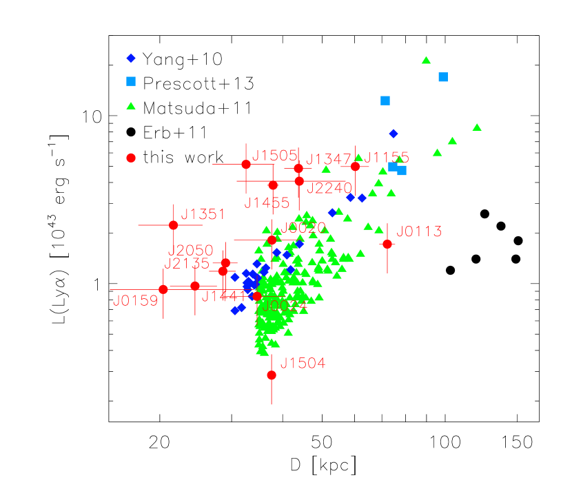
Figure 5: Qualitative comparison of LAB sizes and luminosities. The data have different selection functions and size definitions (see text). Our sample is shown by the red dots. Therein, the lower and upper ends of the vertical error bars represent fractions of 50 and 100 per cent of the FUV flux being caused by Ly $\alpha$, the data points are drawn at 75 per cent.

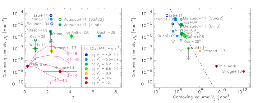
Figure 6: Left: Comoving density of LABs ($L_{{\rm Ly}\alpha}\geq 10^{43}$ erg s^-1, $D\geq 20$ kpc) as a function of redshift. Solid dots represent blind surveys and open dots cluster areas. Horizontal lines show the redshift range covered, vertical lines are the Poisson errors. Arrows represent upper limits. Symbol colours display the survey comoving volumes (see also the right panel). The pink lines show how GBs evolve for different X-ray luminosities if linked to the AGN density evolution (Section 7.2.6). Right: Comoving density as a function of the surveys’ comoving volume. There should be no dependence on volume if the surveys are independent of the environment. The dashed line shows the best fit to the blind surveys at $z=2-4$ (larger filled dots). We kept the colour coding for easier comparison with the left panel.

7.2 Evolution of the LAB comoving density

With our complete sample of GBs, selected from a comoving volume of 3.9 Gpc³ ($z=0.12-0.36$ over 14500 deg² of SDSS), we can for the first time pin down the LAB comoving density, $\rho_{c}$, and its evolution at low redshift. Figure 6 displays $\rho_{c}$ for the GBs and for some high-z LABs from the literature. The symbol colour encodes the comoving volumes probed by the surveys, spanning seven orders of magnitude between $10^{5-12}$ Mpc³. The left panel in Fig. 6 reveals a range of five orders of magnitude in density between surveys. Highest densities are found for (proto-)cluster structures at $z=2-3$ (open symbols), whereas blind surveys (solid dots) yield lower densities. We describe the evolution as a power law, $\rho_{c}\propto(1+z)^{n}$. Our main results are summarized as follows:

• We confirm the previously reported strong evolution below $z=2$; LABs mostly disappear before $z=0.3$. The slope $n$ remains uncertain. It could be as low as $n=1.7$ over $z=4$ to $z=0.3$, or as high as $n=6$ between $z=0.85$ and $z=0.3$.

• High-z and low-z LAB populations are fundamentally different. Most likely, cold accretion streams exhaust sometime between $z=2$ and $z=0.3$. At $z=0.3$, LABs are mostly powered by AGN, and these follow a flatter evolution all the way from $z=4$.

• There is an expected strong dependence of the density on the survey volume, $\rho_{c}\propto V_{c}^{\,-1.6}$. At least Gpc volumes should be probed to appreciate the cosmic large scale structure and cosmic variance, otherwise density measurements from different surveys are difficult to compare.

The following unpublished information has also been used for our analysis: Bridge et al. (2013) have confirmed that all spectroscopically verified LABs in their sample have $L_{\rm Ly\,\alpha}\geq 10^{43}$ erg s^-1. Wold et al. (2014) have confirmed that no other resolved Ly $\alpha$ emitters than the one presented in Barger et al. (2012) are present in their survey. Finally, Matsuda et al. (2011) have provided the full list of LABs including those with diameters less than 100 kpc. We combine their cluster field (SSA22Sb1) and the adjacent fields (SSA22Sb2-7) into one data point and consider it a cluster field (“Matsuda+11 (SSA22)”); we refer to their comparison field survey as “Matsuda+11 (blind)”.

7.2.1 Selection effects and biases

There is currently no definition for LABs (see e.g. Steidel et al., 2011). For this analysis we require a minimum diameter of $D\geq 20$ kpc and a minimum luminosity of $L_{\rm Ly\,\alpha}\geq 10^{43}$ erg s^-1. The latter is a safeguard against completeness issues, biasing us against LABs with low Ly $\alpha$ escape fractions. 13 of the 17 GBs are retained within these limits. Most surveys used for our comparison are sensitive to several $10^{42}$ erg s^-1, and thus should have picked up most LABs with $L_{\rm Ly\,\alpha}\geq 10^{43}$ erg s^-1  in their search volumes. The broad-band survey of Prescott et al. (2012, 2013) is an exception, as only the brightest and largest LABs are detected. We then count how many LABs in the comparison surveys fulfil our criteria, and we recompute the comoving volumes and densities according to our cosmology. For some surveys only a sub-sample of the LAB candidates was followed up spectroscopically, and the total number is extrapolated from the fraction of verified sources. We adopt these correction factors whenever available (e.g. Prescott et al., 2013; Bridge et al., 2013).

Constraining the density evolution is complicated by heterogeneous surveys and selection functions: Matsuda et al. (2011), Saito et al. (2008) and Yang et al. (2009) use narrow-band imaging to select Ly $\alpha$ directly, and Prescott et al. (2012) use broad-band imaging. Spectroscopy is chosen by Keel et al. (2009), Barger et al. (2012) and Wold et al. (2014), whereas Bridge et al. (2013) select dusty Ly $\alpha$ emitters using MIR data. Lastly, our LABs were selected based on their [O iii] strength in $r$-band. We did not correct for any such selection effects. Further biases arise due to cosmic variance (Yang et al., 2009) and because of the original purpose of a survey (clusters, empty fields, etc). We analyse the density evolution separately for blind surveys and cluster surveys.

Lastly, LABs with different ionization sources (cold accretion, AGN, etc.) evolve differently and should be studied separately. However, determining the power source(s) of individual LABs is notoriously difficult (Section 1). We ignore this issue for the moment and address it in Section 7.2.6.

7.2.2 Representative surveys require $10^{8}$Mpc³ volumes

Ideally, measurements of the comoving density are independent of the survey volume. If objects such as LABs are rare, and preferentially found in certain environments such as clusters, then the search volume must be large to become representative. The colour coding in the left panel of Fig. 6 shows that this is not the case for most LAB surveys. We illustrate this in the right panel of Fig. 6, plotting the density as a function of volume. Based on the blind surveys at $z=2-4$, excluding surveys with upper and lower limits and the work of Bridge et al. (2013), we find $\rho_{c}\propto V_{c}^{\,-1.6\pm 0.5}$ (dashed line). In particular narrow-band surveys are observationally expensive when it comes to probing large volumes, as they cut out thin redshift slices, only.

Most current search volumes do not appreciate the full cosmic environment required to produce LABs. How big should these volumes be? LABs with $L_{\rm Ly\,\alpha}\geq 10^{43}$ erg s^-1  and $D\geq 20$ kpc are rare objects at $z\sim 2-4$. They are preferentially found in massive structures with masses of up to $10^{15}$ $M_{\odot}$ (Palunas et al., 2004; Matsuda et al., 2011; Erb et al., 2011; Kubo et al., 2015), which will evolve into the richest clusters known today. What is the volume density of such massive clusters? Ebeling et al. (2001) have compiled a statistically complete sample of the most massive X-ray selected clusters between $z=0.3-0.7$, for which we calculate an average weak lensing mass of $(1.3\pm 0.4)\times 10^{15}$ $M_{\odot}$ based on the data of Applegate et al. (2014). We derive the clusters’ comoving density as $3.8\pm 0.4$ Gpc^-3. To be fully representative of the environment, an LAB search volume should therefore contain at least one Gpc³. However, much smaller volumes of 0.1 Gpc³ should be sufficient when studying the LAB density in the field, e.g. when probing the fast evolution between $z=0.5-1.5$ (Section 7.2.4).

Our subsequent analysis of the LAB density evolution is limited by this effect. We apply approximate corrections when meaningful.

7.2.3 Previous evidence for rapid density evolution

Barger et al. (2012) have searched 0.7 deg² of the Chandra Deep Field South for Ly $\alpha$ emitters between $z=0.67-1.16$ using GALEX grism images. They have found only one extended source at $z=0.977$ with $L_{\rm Ly\,\alpha}=7.2\times 10^{42}$ erg s^-1  and $D=120$ kpc. This was the lowest redshift LAB known so far. For comparison, J1155$-$0147 ($z=0.306$) in our sample is nine times more luminous (Table 3) while having $D=65$ kpc (in [O iii]). Wold et al. (2014) have extended the survey of Barger et al. (2012) to four times the area, but have not found any other resolved Ly $\alpha$ emitters.

To study the evolution of LABs in clusters, Keel et al. (2009) have conducted a GALEX grism search between $z=0.64-1.25$ toward two massive clusters. Numerous LABs (like in Matsuda et al., 2004) should have been found in the absence of evolution, yet none was discovered. Keel et al. (2009) have concluded that the LAB density in clusters must be evolving at least as fast as $n=3.0-3.5$ between $z\sim 0.8$ and $z=2-3$.

7.2.4 LAB density evolution in the field

For the moment, we marginalize the nature and powering sources of LABs, and we neglect the work of Bridge et al. (2013) (see Section 7.2.7). Our survey is a blind survey at $z=0.3$. In comparison with the blind surveys of Saito et al. (2008), Yang et al. (2009, 2010) and Matsuda et al. (2011) we find $n=2.3\pm 1.0$ for $z=0.3-4$, using an unweighted fit. Comparing against Yang et al. (2009, 2010) only, the evolution accelerates to $n=3.6\pm 1.2$ between $z=2$ and $z=0.3$. Comparing our result to the upper limit of Wold et al. (2014), only, the evolution could have been as fast as $n\sim 4$ between $z=0.85$ and $z=0.3$.

Unfortunately, the sampling between $z=0.4-1.5$ is sparse, and it is this interval of cosmic time when $99-99.9$ per cent of the LABs disappear.

7.2.5 LAB density evolution in clusters

At high redshift, LABs are preferentially found in massive structures with masses of up to $10^{15}$ $M_{\odot}$. These systems evolve into the most massive clusters known at low redshift. However, the majority of our low-z LABs are found in isolation or small groups. Only four of them (J1155$-$0147, J1505+1944, J2050+0550, J2202+2309) are in “denser” environments with masses of up to a few $10^{13}$ $M_{\odot}$.

Have we possibly missed LABs in massive clusters due to selection effects? We do detect luminous EELRs if superimposed on brighter ellipticals (e.g. J1504+3439 and J2202+2309 with $M_{i}\sim-22.5$ mag). However, we would not detect them on top of BCGs in the most massive clusters, as the [O iii] EW would become too small to distinguish the galaxies in broad-band colour space (Fig. 1). Some BCGs in massive clusters host emission-line nebula, powered by AGN outflows, starbursts or cooling flows from the IGM. For a few of them Ly $\alpha$ luminosities are known. Hu (1992) find $L_{\rm Ly\alpha}=(1-5)\times 10^{41}$ erg s^-1  for clusters at $z=0.02-0.06$, including NGC 1275A, the BCG of the Perseus cluster. This is a factor of $\sim 100$ below the typical Ly $\alpha$ luminosities of GBs. Going to $z=0.06-0.29$, O’Dea et al. (2004, 2010) find $L_{\rm Ly\alpha}=(0.3-2.8)\times 10^{43}$ erg s^-1  for 9 massive clusters with a median of $0.56\times 10^{43}$ erg s^-1  that is at the bottom of the GB Ly $\alpha$ luminosity function. Abell 1835 ($z=0.253$) is the most luminous system in their sample, reaching about half the luminosity of the most luminous GBs. Such objects would not normally be considered as LABs because of their strong continuum.

Given our non-detection, we conclude that LABs are largely absent in clusters with $M_{200}\gtrsim 10^{14}$ $M_{\odot}$ (unless they are superimposed on the most massive BCGs). This corresponds to an upper limit of $\rho_{c}\sim 2.5\times 10^{-10}$ Mpc^-3 for clusters at $z\sim 0.3$, integrated over our entire survey volume. However, we cannot compare this directly with the densities for clusters at $z=2-3$ (Palunas et al., 2004; Matsuda et al., 2011; Erb et al., 2011) due to the environmental dependency of the latter studies caused by their small search volumes. Statistically, the density of clusters with masses $\gtrsim 10^{15}$ $M_{\odot}$ at $z=0.3-0.7$ is $3.8$ Gpc^-3 (Section 7.2.2). We expect 15 such clusters in our search volume. If at most one of them contains a LAB, then we have a conservative upper limit of $\rho_{c}<3.5\times 10^{-8}$ Mpc^-3 over the same search volume as Matsuda et al. (2011). This yields a slope of $n>2.8\pm 0.6$, compared to $n>3.0-3.5$ obtained by Keel et al. (2009).

We conclude that, like in empty fields, the conditions that support LABs in dense environments at $z\sim 2$ do not hold anymore at low redshift. This implies that cold accretion streams are important at high redshift when pristine gas is still abundant in the IGM, whereas they must have been nearly depleted at low redshift.

7.2.6 Differential evolution of LABs, or how many GBs do exist at high redshift?

We have shown that (1) only LABs in low density environments survive redshift evolution, (2) that low-z LABs are powered by AGN (Section 5.4.1), and (3) that cold accretion streams have likely ceased at $z\sim 0.3$. Consequently, the low-z LAB population is profoundly different from the high-z population, for which accretion streams abound. If the low-z population of AGN-powered LABs (i.e. the GBs) exists independently of the high-z population, how many GBs would we expect at high redshift? In the following consideration we ignore the possibility that high-z LABs, powered by both AGN and cold accretion, could become pure AGN-powered LABs at low redshift. We also ignore AGN flickering which moves individual AGN across luminosity bins. And we assume that the occurrence of an AGN-related GB phase is independent of redshift.

If the GB phase is a (short-lived) phenomenon common amongst active galaxies, then the GB volume density is tied to the evolution of the AGN volume density. The latter is well known (e.g. Ross et al., 2013; Miyaji et al., 2015) for different AGN X-ray luminosity bins. We predict the GB volume density using Fig. 6 in Miyaji et al. (2015) for redshifts $z=1-4$. The predictions are shown by the pink lines emerging from our data point in the left panel of Fig. 6. With the exception of the most luminous bin, it is evident that this evolution is much flatter than the evolution of “typical” high-z LABs.

If GBs adhere to the lowest luminosity bin, log$(L_{x})=42-43$, then with respect to $z=0.3$ their density would be unchanged at $z=1$ and dropped by a factor of 10 at $z=3$. For the second lowest bin, log$(L_{x})=43-44$, the density would remain constant within a factor of 2 out to $z=3$. For the two brightest bins, the density would increase significantly by factors $3-10$ at $z=1$. If GBs were represented by the brightest bin only, then their density would increase further by a factor 50 at $z=2-3$.

Now we can estimate how many high-z GBs have been found by previous LAB surveys. For the volume probed by Yang et al. (2009), we expect 0.001, 0.01, 0.06 and 0.4 GBs for the four bins of increasing X-ray luminosity, respectively. For the blind survey part of Matsuda et al. (2011) we expect 0.0006, 0.005, 0.05, and 0.3 GBs. However, these surveys have found 4 and 21 LABs, respectively, that match our selection criteria ($D\geq 20$ kpc, $L_{\rm Ly\,\alpha}\geq 10^{43}$ erg s^-1). For the broad-band survey of Prescott et al. (2013) we find 0.02, 0.1, 1, and 6 GBs, averaging over the survey’s large redshift range, and based on a sub-sample of GBs with $L_{\rm Ly\,\alpha}\geq 5\times 10^{43}$ erg s^-1  detectable by this survey. Prescott et al. (2013) extrapolate that 18 such LABs exist in their volume. We conclude that it is unlikely that GBs have been detected in any current high-z survey, unless the survey volume exceeds $10^{7}$ Mpc³ and GBs belong to the intrinsically most luminous AGN (currently they are in a low state).

7.2.7 Comparison with Bridge et al. (2013)

Now we can also better interpret the comoving density of Bridge et al. (2013), with $1.1\times 10^{-9}$ Mpc^-3 $100-10000$ times below that of other measurements at $z=2-4$ (Fig. 6). The MIR approach chosen by Bridge et al. (2013) selects LABs with dusty AGN, most of them between $z=1.6-2.8$. X-ray observations of a representative large sub-sample are not yet available. Stern et al. (2014) have observed 3 of the sources (one of which an LAB). They argue that high MIR fluxes and low X-ray counts favour Compton-thick obscuration over intrinsically weak sources; variability is not considered (see also Section 3.4). Larger samples are required to characterize this population of LAB/AGN.

The left panel of Fig. 6 shows that GBs would evolve to similar volume densities at $z\sim 2$ for log$(L_{X})=42-44$. It is plausible that at least some of the LABs described by Bridge et al. (2013) and the GBs belong to the same physical population. Bridge, C.R. report that the Ly $\alpha$ emission of their LABs is rather filamentary based on the extent of the emission measured at various position angles (priv. comm.). This would also be the case for our GBs, a large fraction of which reveals elongated outflows. Another commonality is that both populations are unusually red in the MIR, although for GBs this is based on the W3 and W4 passbands (S13) compared to W1 and W2 for Bridge et al. (2013).

7.2.8 Meeting the postulation of Overzier et al. (2013)

Overzier et al. (2013) argue that most luminous LABs with $L_{\rm Ly\,\alpha}\gtrsim 5\times 10^{43}$ erg s^-1 harbour obscured AGN, and that these AGN are responsible for most of the ionization in the LABs. They consider that “If the luminous LAB phenomenon is associated with powerful AGNs, we would naively expect that the population of LABs should extend toward much lower redshifts […]”. Since the colder gas-rich conditions of $z\sim 2$ proto-clusters, in which the most luminous LABs are found, are replaced by a hot intracluster medium at $z\lesssim 1$, Overzier et al. (2013) suspect that “[…] luminous LABs at low redshift may still be found in the more typical, lower density, and gas-rich environments of actively accreting galaxies and AGNs.”.

This is a spot-on prediction of the properties of our low-z LABs: 85 per cent have Ly $\alpha$ luminosities in excess of $10^{43}$ erg s^-1, 75 per cent are found in isolation or with a small number of companion galaxies, the remaining 25 per cent are found in low mass groups with low concentration. And lastly, all of our LABs harbour AGN.

7.3 Are there type-1 Green Beans, and Green Beans with currently active AGN?

Our optical broad-band selection criteria (Section 2.1.2) favour absorbed (type-2) AGN; unobscured AGN would reduce the observed EW of [O iii] by means of their high continuum fluxes, making the galaxies integrated colours inconspicuous. An unobscured AGN would also partially or fully outshine the EELRs, and the latter would be difficult to recognize without PSF subtraction.

The observed obscuration of an AGN strongly depends on the observer’s viewing angle (Antonucci, 1993), and therefore unobscured (type-1) GBs must exist as well. It is also well-known that the fraction of obscured AGN decreases with increasing X-ray luminosity (e.g. Merloni et al., 2014). Our work, and that of e.g. Hopkins & Quataert (2010); Novak et al. (2011); DeGraf et al. (2014); Schawinski et al. (2015) show that high amplitude X-ray flickering is an inherent property of AGN. This suggests that intrinsic obscuration is also variable and roughly contemporal with the burst duration. The details are beyond the scope of our paper. We expect that unobscured low-z LABs (or type-1 GB analogs) must exist in our SDSS search volume, perhaps as many as described in this work.

The following question must be seen in the same context: How many GBs exist with their AGN still being in the high state, and how would they look like? Binette & Robinson (1987) have shown that [O iii] responds nearly instantaneously to a change of ionizing radiation, at least when considering volumes with kpc scales such as in GBs. That means that the life-time of an observable GB phase is tightly linked with the life-time of the AGN bursts; a strong ionization echo is only observed as long as the ionizing radiation from a previous high state is still escaping the galaxy. Therefore, the ratio of galaxies that appear as echoes (GBs) and their progenitors (with the AGN still in a high state) is similar to the ratio of the AGN fading time-scale and the duration of the AGN high state. Both occur on scales of thousands to hundreds of thousands of years (this work, and Hopkins & Quataert, 2010; Novak et al., 2011; DeGraf et al., 2014; Schawinski et al., 2015). It is plausible that there might be $1-100$ times as many GB “progenitors” as GBs themselves. As argued above, the optical appearance of the progenitors (and their obscuration) is likely to change (see also the changing look quasars LaMassa et al., 2015; Runnoe et al., 2016); we expect galaxies with brighter nuclei, making it more difficult to recognize their EELRs.

Imaging surveys with greater angular resolution than SDSS (e.g. LSST) would simplify the identification for unobscured GBs and their progeenitors. They are likely already contained in public quasar catalogues because of their high fluxes ($r\lesssim 18$ mag).

8 Summary and conclusions

Green Bean galaxies (GBs, $z\sim 0.3$) are spectacular and the most powerful emission-line objects known in the nearby Universe. Their extended emission-line regions (EELRs) measure between $20-70$ kpc, and they are ionized by radio-weak type-2 quasars. GBs are extremely rare with a surface density of $1.1\times 10^{-3}$ deg^-2; only 17 of them are known. They were selected photometrically from the 14500 deg² footprint of SDSS-DR8. In S13 we have suspected that the EELRs are ionization echoes, i.e. the AGN have faded recently and more quickly than the EELRs’ typical light crossing times. GBs have not been investigated further apart from the single case study of Davies et al. (2015),

In this paper we have presented multi-wavelength observations to understand the unusual nature of GBs and to view them in the context of galaxy evolution. With Chandra we have probed the current activity of the AGN and the intrinsic obscuration along the line of sight toward 10 GBs. With GALEX archival images we have estimated the far-UV properties of 15 GBs, and we have obtained high resolution optical images in $gri$ filters for all objects.

8.1 Main results

1. Chandra has revealed low counts, moderate hardness ratios and weak or absent K$\alpha$ lines. This implies that these AGN are intrinsically weak rather than Compton-thick. The EELRs’ high [O iii] luminosities require recent and rapid fading of the AGN, confirming them as ionization echoes (Section 3.4).

2. Strongly variable AGN do not follow the MIR X-ray relation. The MIR response of a dusty torus can be delayed by up to $\sim 10^{3}$ years (Hönig & Kishimoto, 2011), forming a thermal echo. Accordingly, the AGN in the GBs must have faded by several factors $10-100$ over the last $100-1000$ years (Section 6.4.1). Combining the thermal and ionization echoes, the AGN must have faded by $3-4$ orders of magnitude within the last $10^{4-5}$ years. This rate is similar to that observed in the changing look quasars (LaMassa et al., 2015; Runnoe et al., 2016, also attributed to change of accretion rates); however, in GBs it could be sustained over much longer periods of time.

3. GALEX FUV images require that at least 85 per cent of the GBs have Ly $\alpha$ luminosities in excess of $10^{43}$ erg s^-1. They form Lyman-$\alpha$ blobs or LABs (Section 4 and 7.1). We have proven that LABs still exist in the Universe $4-7$ billion years later than previously known. Ultimately, the Ly $\alpha$ emission has to be confirmed with FUV spectroscopy using HST or Astrosat (Hutchings, 2014).

4. We propose rapid duty cycles (AGN flickering) as a natural explanation for the mysterious ionization deficits observed in LABs. Resonant Ly $\alpha$ photons are efficiently stored in LABs and only gradually released, decorrelating from AGN variability on scales of up to $10^{6}$ years depending on the optical depth. An AGN may undergo several duty cycles before Ly $\alpha$ escapes; a luminous LAB does not require a currently powerful AGN, independent of obscuration (Section 6.3). This does not mean that we can relinquish e.g. cold accretion, star formation and shocks as ionization sources. It means that multi-wavelength observations are required to identify the ionizing source(s) of individual LABs.

5. Low-z LABs live mostly in isolation or in low density environments (Section 5.1), whereas high-z LABs are preferentially found in massive structures. Sometime between $z=2$ and $z=0.3$ these structures must lose their ability to form and sustain LABs, probably because cold accretion streams have depleted. AGN survive, and may continue powering LABs at low redshift (Section 5.4.1).

6. Our comoving volume is 3.9 Gpc³, $100-1000$ times larger than other LAB surveys, second only to Bridge et al. (2013). The density at $z\sim 0.3$ is $\rho_{c}=3.3\pm 0.9$ Gpc^-3 for LABs with $L_{\rm Ly\,\alpha}\geq 10^{43}$ erg s^-1  and $D\geq 20$ kpc. The density evolves with $\rho_{c}\propto(1+z)^{3-4}$ for both clusters and in the field between $z=0.3$ and $z=2$. During this time, $99-99.9$ per cent of the LABs disappear. A more accurate determination of the evolution requires (1) better sampling between $z=0.5-1.5$, and (2) volumes of $0.1-1$ Gpc³ to overcome cosmic variance and to be independent of environment. Otherwise, densities are not directly comparable (Section 7.2.2).

7. LABs with different ionization sources evolve differently. Gravitationally powered LABs do not survive redshift evolution as the cold accretion streams are depleting. We find only one LAB, J1155$-$0147 ($z=0.306$), that could still be powered by cold streams in addition to an AGN. The density of LABs powered solely by AGN is evolving much slower, if at all, depending on the AGN’s intrinsic X-ray luminosity (Sects. 7.2.6 and 7.2.7).

8.2 Conclusion and future observations

LABs should be considered as efficient Ly $\alpha$ photon stores, albeit with a badly maintained inventory. They trap Ly $\alpha$ photons for a time much longer than their light crossing time. When the thermalised photons are eventually released in a gradual manner, all memory about the location, spectrum and time variability of their source has been lost. Typical storage times are short compared to the life times of cooling flows, star bursts, and shock ionization populating the store with photons. However, the storage times become long compared to episodic AGN bursts and their transition from high to low states (and vice versa). Even if optical and MIR observations point to the most powerful AGN, the absence of the latter in X-rays does not necessarily mean Compton-thick obscuration.

The AGN timescale is much shorter than the typical galaxy time-scale and the galaxies response time to AGN activity; care must be taken when seeking or applying relations between AGN and other “galactic” observables, in particular if the AGN are suspected to be transient (see also Hickox et al., 2014).

The GBs and the associated LABs published in this paper are much easier to study than their high-z counterparts, as low fluxes, redshift incompleteness, and physical resolution are not a problem. They are perfectly suited to study AGN feedback, large-scale outflows, quasar duty cycles, mode switching, and the Ly $\alpha$ escape fraction, the latter being controlled by an interplay of geometry and velocity field, metallicity, hydrogen density, dust obscuration and AGN variability.

Our own NUSTAR observations have commenced in cycle 2 for the two X-ray brightest GBs, J1155$-$0147 and J0113+0106, to accurately determine the obscuration and the actual shut-down “depth” of their AGN. Time has also been awarded for an initial survey with the Hubble Space Telescope, to determine the FUV properties of the same two GBs, and J2240$-$0927 (Davies et al., 2015), using ACS/SBC imaging and spectroscopy.

Appendix A Notes about individual targets

A.1 J0020–0531 (z=0.334)

The strong [O iii] emission mimics the widely opened arms of a SBc galaxy. The gas has high surface brightness in the centre, and appears tidally warped by two nearby elliptical galaxies at the same redshift. It is not clear whether the gas in the two ’arms’ is outflowing due to AGN activity, infalling, or pulled out by tidal forces. It could be forced into the spiral shape by differential rotation. The projected distances to the two elliptical galaxies are 11 and 24 kpc, respectively. Fan-shaped tidal debris, consisting of stars and/or gas, extends southwest over 35 kpc, embedding one of the ellipticals. The host galaxy is compact.

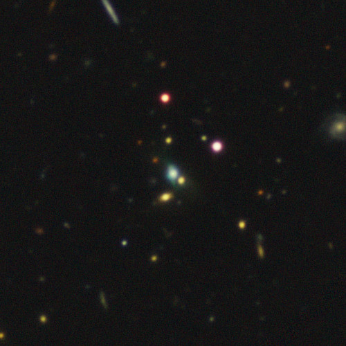
Figure 7: J0020–0531. The images of the GBs in this Appendix are true-colour renditions of the $gri$ data. The powerful [O iii] line dominates the green channel. A selective non-linear stretch was applied to the GBs to avoid saturation; they are significantly brighter with respect to the other field galaxies than these images suggest.

A.2 J0024+3258 (z=0.293)

This system has a complex, disrupted morphology. The [O iii] emission is high in the centre. A collimated bipolar outflow extends over a total of 31 kpc in North-South direction. It gets wider with distance from the nucleus, and shows a twist beginning about halfway from the centre. It is probably ionized by a double ionization cone. Tidal debris of stellar origin (judged by its broad-band colours) intersects the outflow at an angle of about 45 degrees. It extends over at least 54 kpc and increases in surface brightness toward the nucleus.

The $gri$ colour image reveals several ellipticals and red spirals with similar colours as the tidal debris. However, our long-slit spectra reveal that they belong to an unrelated foreground structure at $z=0.22$. J0024$+$3258 is an isolated, advanced merger system in a low density environment.

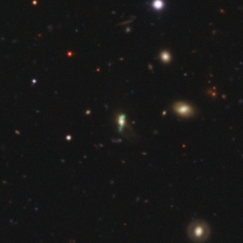
Figure 8: J0024+3258

A.3 J0111+2253 (z=0.319)

This galaxy is dominated by a 22 kpc long luminous unipolar outflow to the Southeast. A fainter outflow of similar extent is visible to the South. The host galaxy is compact. 35 kpc to the East of J0111+2253 is an elliptical galaxy at $z=0.321$. Their relative radial velocities are $450\pm 220$ km s^-1. Both galaxies are symmetrically embedded in a diffuse halo stretching in a slightly curved manner over 103 kpc from East to West, and over 23 kpc North to South. The colours of this halo and of the elliptical galaxy are the same. These galaxies must have experienced a close encounter in the past.

Another elliptical galaxy 92 kpc south of J0111+2253 is at the same redshift. The field shows several other galaxies with unknown redshifts. The overall impression is that of a low density environment.

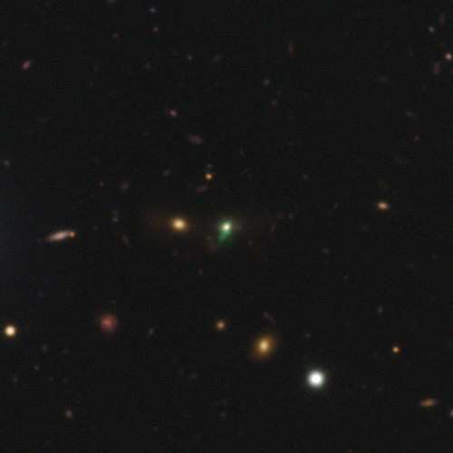
Figure 9: J0111+2253

A.4 J0113+0106 (z=0.281)

A spectacular system with two symmetric luminous [O iii] superbubbles on the northwestern and southeastern side of the nucleus, at a projected distance of 5.5 kpc each. The northwestern bubble is somewhat fainter than the one in the Southeast, and their diameters are $5-8$ kpc. There is also a 14 kpc long curved arc in [O iii] at 24 kpc separation from the nucleus. It is connected with the main system through a fainter [O iii] bridge. This could be an old ejecta from the AGN, or gas pulled out by tidal interaction. There is no galaxy visible in this arc, suggesting an AGN-driven outflow. The curvature of this arc and the misalignment with the two superbubbles is remarkable. In the absence of a shaping radio-jet this could perhaps indicate a nuclear spinflip, e.g. caused by an SMBH merger. It is evident that this AGN underwent at least two powerful events in the past. The youngest one, perhaps $2-5$ million years ago, ejected the two superbubbles. An older event $20-30$ million years ago sent out the arc, and possibly some very faint [O iii] emission out to 43 kpc south of the nucleus, roughly aligned with the two superbubbles. At the moment this is qualitative at best, as we have no radial velocities nor information about the true orientation in space.

The entire system, 16 arcsec wide, is embedded in a low surface brightness halo whose colours suggest a stellar origin. The nucleus of J0113$+$0106 is also very luminous in [O iii] and makes it difficult to discern the host galaxy. The latter could be a compact elliptical, given the somewhat redder colours of the centre. A second compact elliptical with a diameter of 6 kpc is found at a projected distance of 8 kpc to the West of the nucleus. Its redshift is still unknown and this could be a chance projection. Regardless, J0113$+$0106 is a rather isolated system. There is a sparse foreground galaxy cluster at $z=0.186$ to the North.

Overall, J0113+0106 is reminiscent of SDSS J1356+1026 at $z=0.123$, where a pair of 10 kpc outflows is found by Greene et al. (2012). Both systems are also radio-quiet.

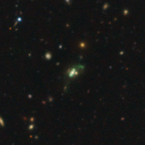
Figure 10: J0113+0106

A.5 J0159+2703 (z=0.278)

This is a rather untypical GB because the emission-line region is hosted in a 46 kpc size, bright spiral galaxy with a pronounced bar. In addition, or because of this, the [O iii] EW is lower than in other GBs. A long-slit observation for our field spectroscopy survey intersects the outer areas of this galaxy and we detect [O iii] out to 25 kpc from the nucleus. The barred spiral is not visible in the SDSS images in which this object was discovered.

Field spectroscopy shows that J0159$+$2703 is relatively isolated. Only one elliptical at 590 kpc separation has so far been confirmed at the same redshift. Two more, smaller ellipticals of the same colour, and a few spirals are still pending redshift confirmation.

J0159$+$2703 has a mid-IR flux (18.1 mJy) close to the median of our sample (Table 2), yet its X-ray count rate is by far the lowest. This could indicate an exceptionally strong fading of the AGN in recent times.

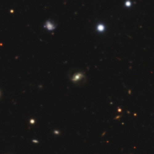
Figure 11: J0159+2703

A.6 J1155–0147 (z=0.306)

This galaxy is extraordinary. First, its [O iii] emission has a diameter of 64 kpc and is the largest nebula in our sample. It also has the highest GALEX FUV luminosity, the highest X-ray counts and relatively low column density (see Section A.6.1). The host galaxy is likely an elliptical.

The [O iii] emission roughly decomposes into three main parts: a luminous centre with a diameter of 12 kpc, a medium-bright and somewhat elliptical zone of 30 kpc, and a fainter envelope extending over 64 kpc. The latter has a characteristic ’X’-like shape, which could either be caused by a strong bipolar and older ionization cone, preferentially oriented in the plane of the sky, or it is simply a direct consequence of the spatial distribution of the gas. Ionizing radiation appears to escape in all directions as evidenced by the central surface brightness distribution.

A fragmentation into smaller clouds lends an unusual, mottled appearance to J1155$-$0147. The typical diameter of these clouds is about 0$.\!\!^{\prime\prime}$8 to 1$.\!\!^{\prime\prime}$6 or $3.5-7.0$ kpc. We count $12-16$ of them. Possibly, the AGN has sputtered outflows in various directions during several duty cycles. Precession of a single or binary SMBH could also be responsible for the clouds and the ‘X’-like shape.

Another possibility is that the smaller clouds are shock-compressed regions in infalling gas. Interestingly, J1155$-$0147 is located at the geometric centre of a low mass galaxy group. The group has at least a dozen members, mostly ellipticals and red spirals, distributed over $\sim 220$ kpc. Using the mass-richness relation for red sequence galaxies (Hansen et al., 2005, 2009; Johnston et al., 2007), we estimate the total mass to $M_{200}=(1.3\pm 0.9)\times 10^{13}\;M_{\odot}$. There is no indication of a soft X-ray group halo in the Chandra data. None of the other member galaxies are seen in X-rays. The major axis of the [O iii] emission is aligned to within 20 degrees with the major axis of the galaxy distribution. Possibly, some cold accretion is still happening in J1155$-$0147, similar to the LABs of Erb et al. (2011) which are preferentially aligned with filaments. The smaller clouds are of similar size and reminiscent of the structures seen in the Ly $\alpha$ fluorescence maps of Kollmeier et al. (2010) that arise in cold accretion streams. It is unclear, though, whether these Ly $\alpha$ structures would also reflect in [O iii].

Another odd feature is a broad tidal stream, $15x35$ kpc in size, extending from the elliptical galaxy J115545$-$014722 in direction to J1155$-$0147 (90 kpc away, clearly visible in Fig. 12). Our central long-slit spectrum of this galaxy does not reveal any emission lines. A possible dynamic encounter with J1155$-$0147 would have occurred $\gtrsim 200$ million years ago if $200$ km s^-1is the typical velocity of the cluster members. Likely, the two phenomena are not directly linked.

If the [O iii] nebula is outflowing, then this object would contribute significantly to the enrichment of the intergalactic medium in this group. The contrast between the essentially gas depleted ellipticals and the gas-rich GB in the group centre is remarkable.

A curious comparison that comes to mind is that of the Phoenix cluster (Williamson et al., 2011; McDonald et al., 2012) at $z=0.596$, where a massive cooling flow on to the BCG feeds a substantial star burst (McDonald et al., 2015). The authors also argue that the type-2 quasar present in the BCG is currently transition from a high state into a low state (like the GBs), given the simultaneous presence of radiative and kinematic feedback. A more detailed comparison of these two systems is worthwhile, given their similarities despite their vastly different environments.

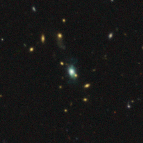
Figure 12: J1155–0147

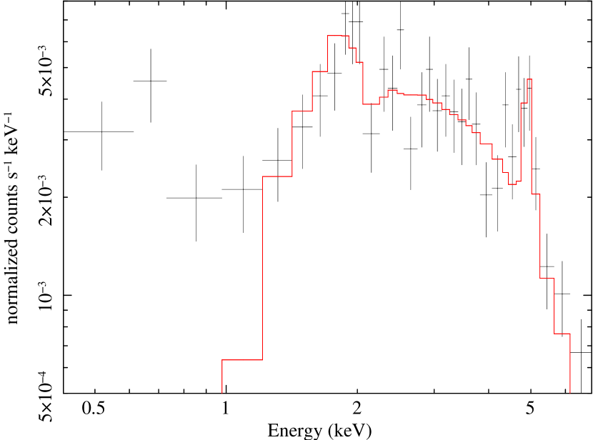
Figure 13: Chandra spectrum of J1155-0147. The background-subtracted spectrum binned into groups of a minimum of 20 counts (black crosses) is fit with a power law and the spectrally unresolved Fe K$\alpha$ line at 6.4 keV in the galaxy’s rest frame (red solid line). The low-energy spectrum is fit poorly, suggesting that an additional physical component is producing the soft X-rays.

A.6.1 Archival Chandra data of J1155-0147

J1155$-$0147 is by far the X-ray brightest of the GBs. The 30 ks Chandra exposure provides a total of 550 counts in the useful energy range, revealing a weakly extended source with a relatively soft spectrum. We fit the full ($0.3-8.0$ keV) spectrum as the sum of the AGN power law with photon index $\Gamma=1.9$, plus the unresolved Fe K$\alpha$ line (Fig. 13). The very soft spectrum below 1 keV is fit poorly, indicating the presence of photoionized emission corresponding to the strong optical [O iii] line. Thermal emission from a starburst is unlikely because of the high value of ${\rm log([\textup{O\,{iii}}]/{\rm H}\beta)=1.163\pm 0.006}$ (S13), requiring a hard spectrum. We recover the AGN in this fit with an intrinsic flux $F_{0.3-8}^{\rm intr}=1.18\times 10^{-13}$ erg s^-1 cm^-2  and $N_{\rm H}=5.1\times 10^{22}$ cm^-2. The rest frame EW of the Fe line is 500 eV.

A.7 J1347+5453 (z=0.332)

This is a text-book example of an AGN jet and a double ionization cone lighting up a bipolar outflow. As such it is reminiscent of J0024+3258. The host galaxy is a red edge-on spiral with 21 kpc diameter, unresolved along its minor axis. The outflow is launched from the nucleus and nearly perpendicular to the disk.

The southeastern outflow has a smaller opening angle, and after $\sim 5$ kpc it bends by 90 deg and runs parallel to the disk. The northwestern outflow has irregular surface brightness distribution and a wide opening angle of $70-80$ deg. It stretches over at least 12 kpc. At a distance of 18 kpc we find a 4 kpc wide (0$.\!\!^{\prime\prime}$8), faint blob of gas that is mostly visible in the $r$-band image. A weak detection in $g$-band could be caused by [O ii] and [Ne iii] emission. It is also weakly detected in $i$-band. Since H $\alpha$ is redshifted beyond $i$-band, the most plausible emission lines that could cause the $i$-band signal are [O i]$\lambda$6302,66, possibly indicating shock ionization. A high contrast stretch of the $r$-band image reveals that the northwestern outflow reaches further to least 32 kpc from the nucleus, embedding this seemingly isolated blob of gas.

Spectra of field galaxies have not yet been taken. Two ellipticals nearby have similar colours as the edge-on disk in J1347$+$5453, and could be at the same redshift. Overall, this is a low density area.

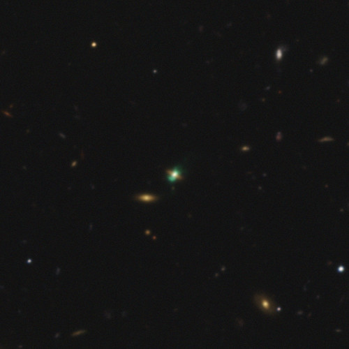
Figure 14: J1347+5453

A.8 J1351+0816 (z=0.306)

Imaging data reveal a featureless, spherically round nebula with symmetric brightness profile peaking at the centre. The sky noise is met at a diameter of 28 kpc. A compact blue star-forming galaxy is superimposed at a distance of 9.4 kpc of the nucleus. We took a long slit spectrum of it and detect a weak continuum and nebular emission lines. The latter place it either at a slightly lower redshift than the host galaxy $(\Delta z=-0.0007)$, or they are due to superimposed gas from the host. No other emission or absorption lines are seen. There is a small chance that this is a high-z galaxy in the redshift desert, or a foreground star. Otherwise, J1351$+$0816 appears to be an isolated galaxy in the field.

Noteworthy is a very faint halo in the $r$-band image (not visible in the images reproduced in this paper; check the public available coadded FITS images) extending 48 kpc to the South. It coincides with our long-slit orientation and we detect [O iii] over its entire extent.

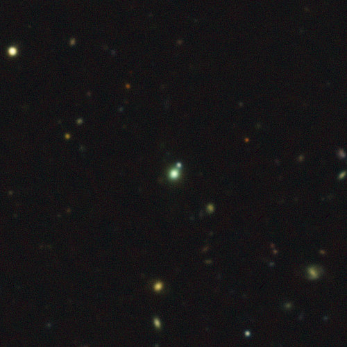
Figure 15: J1351+0816

A.9 J1441+2517 (z=0.192)

This GB has the lowest redshift in our sample. The [O iii] nebula consists of a 7 kpc long bright core elongated North-South. A host galaxy is likely compact. A fainter area of irregular surface brightness stretches over 17 kpc to the North, with an opening angle of approximately 90 degrees. The southern part of the emission-line nebula is weaker and more diffuse than the northern part. Two red compact galaxies of unknown redshift are embedded in the southern nebula. If at the same redshift as J1441+2517, then their physical sizes are 6 kpc and 4 kpc, respectively. Other than that this galaxy would live in isolation. A bridge in the [O iii] nebula appears to connect the larger of the two possible companions with the nucleus of J1441+2517. Judging from its colours, a mix of ionized gas and stellar tidal debris extends 22 kpc to the South of the nucleus, in a broad fan-shaped fashion.

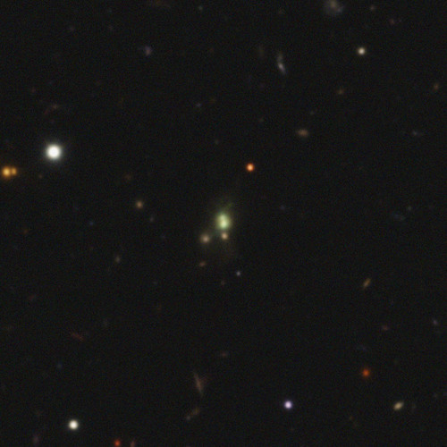
Figure 16: J1441+2517

A.10 J1455+0446 (z=0.334)

This is the most a bizarre system in our sample, extending over 40 kpc. The [O iii] emission is brightest in the nucleus and has two wings that extend in East-West direction. The nucleus appears at the edge of the galaxy. A condensation (probably a star cluster) is seen North of the nucleus. Significant colour gradients suggest a wild mix of tidally disturbed gas and stars, consequence of a violent merger. Spectroscopy of 7 field galaxies yield only one galaxy with similar redshift $(z=0.329)$, making it unlikely that these two galaxies interacted in the past. Otherwise, this redshift difference would imply an encounter with a radial velocity of $\sim 1100$ km s^-1, inconceivable in the absence of a massive cluster. The large spiral to the South is a foreground object at $z=0.087$.

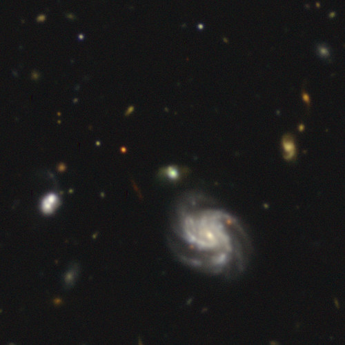
Figure 17: J1455+0446

A.11 J1504+3439 (z=0.294)

The [O iii] nebula in this galaxy is brightest at the nucleus, and fragments into several clouds of medium surface brightness. We find a bubble-like structure extending 12 kpc to the East of the nucleus. Fainter parts reach radii of 18 kpc in different directions. The ionized gas is superimposed over an elliptical galaxy measuring approximately $37\times 24$ kpc. This is the only GB where the gas distribution resembles that of the Voorwerpjes (ionization echoes at $z\lesssim 0.1$) described by Keel et al. (2012b, 2015), with the notable difference that Voorwerpjes are not observed in ellipticals.

The field is populated by about 20 brighter spirals, ellipticals and interacting galaxies loosely scattered across the area. Most of them have SDSS photometric redshifts of $z=0.22-0.40$ ($\Delta z=0.06-0.08$). Spectroscopic redshifts place two galaxies at different distances than J1504+3439. Spectra for three more galaxies have too low S/N for redshift determination, and they are likely at higher redshift.

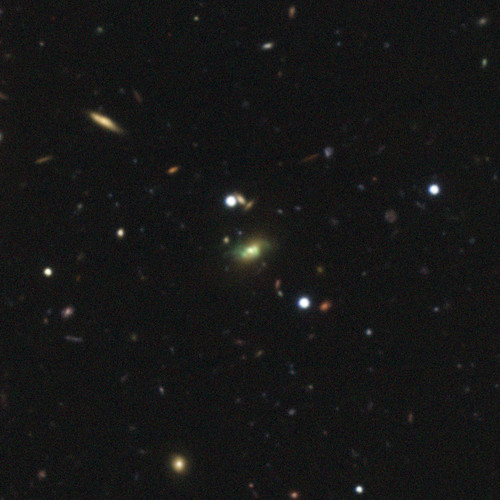
Figure 18: J1504+3439

A.12 J1505+1944 (z=0.341)

This is the highest redshift GB in our sample. Its nebula extends East-West over 28 kpc with high central surface brightness. The eastern wing is brighter than the western wing, in which a small elliptical galaxy is embedded and confirmed at the same redshift. It appears to be tidally interacting with the ionized gas. J1505+1944 is the only GB where the [O iii] and X-ray peaks are significantly offset from each other (see Section 3.2).

J1505$+$1944 is located in a small group of at least 8 spectroscopically verified members. The red sequence has $10-15$ members, mostly small ellipticals within $1.6$ Mpc. The concentration of this group is low. Analogous to Section A.6 we estimate $M_{200}=(4\pm 1)\times 10^{13}\;M_{\odot}$. The host galaxy is compact, and small in comparison to the other group members.

J1505$+$1944 is superimposed on a small group of red ellipticals, likely at $z\sim 0.8-0.9$.

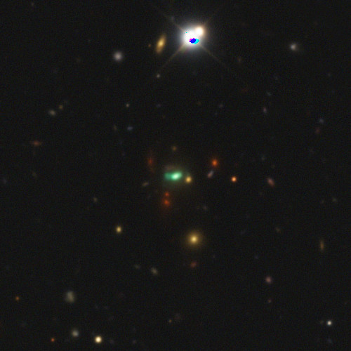
Figure 19: J1505+1944

A.13 J2050+0550 (z=0.301)

J2050+0550 has a smooth EELR with high central surface brightness. A 7 kpc cloud is seen 4.5 kpc to the Northwest, less pronounced yet similar to J2240$-$0927. One of our field long-slit spectra was taken southwest of the nucleus. We still detect [O iii] emission at a radius of $20$ kpc. This shows that the [O iii] sizes listed in Table 4, based on $r$-band surface brightness, may significantly underestimate the true extent of the ionized nebulae. The host galaxy is compact.

$10-12$ red sequence galaxies are found within a radius of about 540 kpc of J2050$+$0550. We obtained spectra for three of them and they have the same redshift as J2050$+$0550. The cluster is sparse, with J2050$+$0550 located near the densest area (similar to J1155$-$0147). None of the other cluster members is detected in X-rays, nor do we see diffuse emission from a cluster X-ray halo. Analogous to Section A.6) we estimate $M_{200}=(2.6\pm 0.8)\times 10^{13}\;M_{\odot}$.

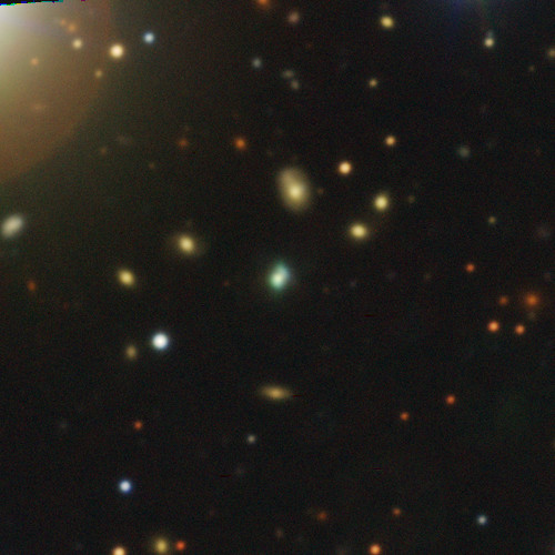
Figure 20: J2050+0550

A.14 J2135–0314 (z=0.246)

The host galaxy of J2135$-$0314 is compact, overpowered by the high nebular central surface brightness. Three fringes lend a tattered look to the nebula. The northeastern fringe curves to the South over $\sim 9$ kpc, the southeastern fringe is straight an can be traced over 13 kpc before disappearing in the sky noise. The galaxy is located in a remarkably empty area. Plausibly interacting companions are not seen.

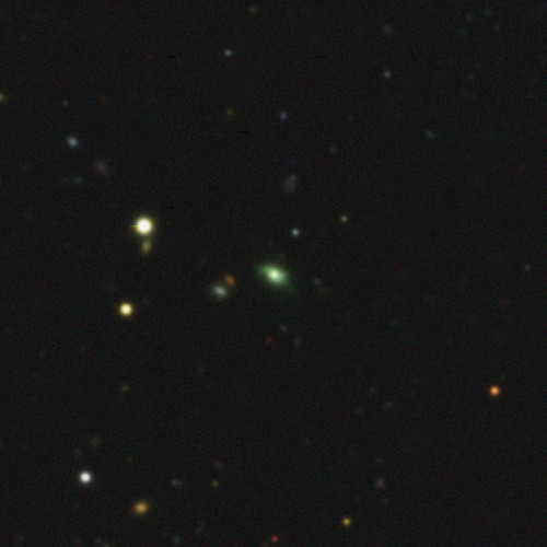
Figure 21: J2135–0314

A.15 J2202+2309 (z=0.258)

J2202$+$2309 is located in a structure with several red sequence galaxies confirmed at $z=0.258$. Our data reveal about 40 red sequence galaxies with matching colours and within 600 kpc radius. However, an unknown fraction of them belongs to a galaxy cluster projected about 330 kpc to the West and with $z\sim 0.230$ (about 80 Mpc in the foreground of J2202$+$2309, neglecting possible bulk motions along the line of sight). Like in case of J1155$-$0147 and J2050$+$0550, the GB is located near the centre of the galaxies at $z=0.258$. More field spectroscopy is required to clarify the structures along the line of sight, and to obtain reliable mass estimates. Assuming a contamination of 50 per cent, this cluster could be as massive as $(5-8)\times 10^{13}\;M_{\odot}$ (see Section A.6), and would be the most massive structure in our survey. This field was not part of our X-ray observations.

J2202$+$2309 differs from the other GBs in the sense that its host galaxy is a luminous ($M_{i}\sim-22.5$ mag) elliptical. The [O iii] emission does not dominate the broad-band colours as much. Tidal disturbances are visible in the halo of J2202$+$2309. The physical extent of the elliptical host is at least $40\times 25$ kpc. A contrast-enhanced $r$-band image shows that this galaxy shares a common faint halo with J220215.5+230859, another elliptical of comparable size and luminosity, and possibly a third elliptical as well. This triple system could form the future BCG of this cluster.

One of our long slit positions has an impact parameter of 12 arcsec (48 kpc) with respect to the nucleus. There is a weak detection of [O iii] over 3 arcsec length at the point of highest proximity to J2202$+$2309. Our 20 minute $r$-band image (containing the redshifted [O iii] line) is not deep enough to reveal a signal at this location. This part of the sky has not been surveyed in the FUV with GALEX.

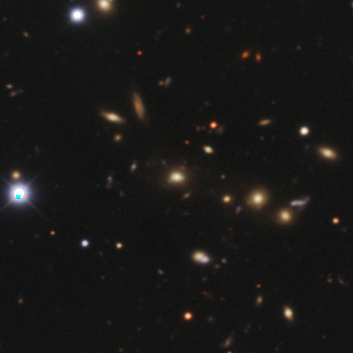
Figure 22: J2202+2309

A.16 J2240–0927 (z=0.326)

This is an interacting system in an otherwise empty area. A detailed study using GMOS-S 3D spectroscopy has been presented in Davies et al. (2015), showing a complex and turbulent merger system with different gas phases and an ionization cone.

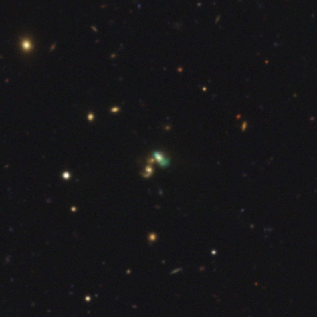
Figure 23: J2240–0927

A.17 J2308+3303 (z=0.284)

This system appears rather normal in our broad-band data, like a face-on spiral with insufficient resolution to discern the spiral arms. The nucleus is bright and barely resolved. Either the nebular flux is concentrated in the nucleus (and therefore within a physical diameter of 6 kpc), or it is more extended but with low EW and of relatively uniform surface brightness. The surrounding featureless disk has a diameter of $22\times 20$ kpc. There is one spectroscopically confirmed neighbour, a distorted spiral, 29 kpc to the North.

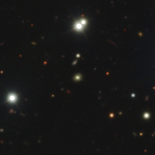
Figure 24: J2308+3303

Table 4: Properties of the optical nebulae and host galaxies. Two estimates of the EELRs’ physical diameters are given in columns 2 and 3: $D_{\rm[\textup{o\,{iii}}]}^{\,\rm min}$ is a lower limit based on the green appearance in $gri$ colour images where [O iii] dominates the $r$-band. $D_{\rm[\textup{o\,{iii}}]}^{\,\rm max}$ is the largest diameter of a contour $2\sigma$ above the sky noise (column 3). Column 4 lists the mean surface brightness along this contour. Column 5 states whether spectra of field galaxies have been taken. Column 6 lists the local environment of the GBs. We consider it a group if at least 2 other galaxies are at the same redshift. Column 7 lists the size estimates of the host galaxies. These are approximate due to the contamination of the broad-band filters by nebular emission. Column 8 is a morphological classification of the hosts, often troubled by the limited spatial resolution in which case we classify them as compact. These could be small ellipticals as well as star-forming galaxies. Column 9 contains our best guess whether these systems are interacting or merging. Column 10 states whether the gas distribution resembles AGN driven outflows. In column 11 we describe the gas distribution and other system characteristics.

Name	$D_{\rm[\textup{o\,{iii}}]}^{\,\rm min}$	$D_{\rm[\textup{o\,{iii}}]}^{\,\rm max}$	${\rm SB}_{S/N=2}$	Spec.	Environment	Host size	Host type	Merger	Outflow	Comment
	[kpc]	[kpc]	[erg s-1 cm-2]	survey		[kpc]
			arcsec-2]
SDSS J002016.44$-$053126.6	30	44	$2.90\times 10^{-16}$	Yes	Group	$18\times 14$	compact	Yes	Yes	Tidally warped outflow; compact group
SDSS J002434.90$+$325842.7	28	40	$1.94\times 10^{-16}$	Yes	Isolated	$10\times 7$	irregular	Yes	Yes	Bipolar outflow
SDSS J011133.31$+$225359.1	21	28	$1.78\times 10^{-16}$	Yes	Group	$18\times 14$	compact	Yes	Yes	Unipolar outflow; sparse group
SDSS J011341.11$+$010608.5	68	75	$2.40\times 10^{-16}$	Yes	Isolated	$8\times 6$	compact	Yes	Yes	Bipolar outflow and signatures for
										recurrent outflows
SDSS J015930.84$+$270302.2	6	33	$1.80\times 10^{-16}$	Yes	Isolated	$46\times 46$	spiral	$-$	$-$	Prominent spiral, one confirmed distant
										neighbour
SDSS J115544.59$-$014739.9	55	65	$2.24\times 10^{-16}$	Yes	Group	$16\times 12$	elliptical	?	?	Perhaps a cold accretion nebula at the
										centre of a cluster
SDSS J134709.12$+$545310.9	40	47	$2.77\times 10^{-16}$	$-$	Isolated / Group	$21\times 4$	spiral	$-$	Yes	Very small group, perhaps $2-3$ members
SDSS J135155.48$+$081608.4	17	25	$2.31\times 10^{-16}$	$-$	Isolated / Group	$14\times 14$	spherical	$-$	$-$	Smooth spherical nebula; Isolated or
										in very sparse group
SDSS J144110.95$+$251700.1	21	27	$2.81\times 10^{-16}$	$-$	Isolated / Group	$\lesssim 6$	compact	Yes	Yes	Multiple faint outflows; two small
										companions (unconfirmed)
SDSS J145533.69$+$044643.2	36	39	$2.24\times 10^{-16}$	Yes	Isolated	$9\times 7$	irregular	Yes	?	Totally disrupted system
SDSS J150420.68$+$343958.2	36	38	$2.33\times 10^{-16}$	$-$	Isolated	$37\times 24$	elliptical	$-$	Yes	Compact clouds superimposed on
										undisturbed elliptical
SDSS J150517.63$+$194444.8	26	38	$3.14\times 10^{-16}$	Yes	Group	$10\times 7$	compact	?	Yes	Recurrent outflows; red sequence
										galaxies, low concentration
SDSS J205058.08$+$055012.8	26	31	$2.23\times 10^{-16}$	Yes	Group	$17\times 16$	compact	$-$	Yes	Smooth with ejected (?) cloud
SDSS J213542.85$-$031408.8	26	30	$2.70\times 10^{-16}$	Yes	Isolated	$8\times 7$	compact	?	Yes	Multiple outflows
SDSS J220216.71$+$230903.1	14	31	$1.66\times 10^{-16}$	Yes	Group / Cluster	$40\times 25$	elliptical	Yes	$-$	Bright elliptical, gas morphology
										not well visible
SDSS J224024.11$-$092748.1	30	56	$1.53\times 10^{-16}$	Yes	Isolated / Group	$9\times 9$	spherical	Yes	Yes	Case study in Davies et al. (2015).
										Two companions, one confirmed.
SDSS J230829.37$+$330310.5	16	25	$1.69\times 10^{-16}$	Yes	Isolated pair	$22\times 20$	spiral	$-$	$-$	Inconspicuous, one nearby member

Table 5: Redshift survey of field galaxies near GBs. The Membership is in parentheses if the galaxy is a foreground/background object.

$\alpha_{2000.0}$	$\delta_{2000.0}$	z	Membership	Spectral features and morphology
00:20:16.333	$-$05:31:28.02	0.334	J0020$-$0531	CaH+K; elliptical
00:20:16.550	$-$05:31:31.54	0.334	J0020$-$0531	CaH+K; elliptical
00:20:19.705	$-$05:32:21.89	0.281	(J0020$-$0531)	CaH+K; foreground elliptical
00:24:24.557	+33:00:24.74	0.204	(J0024+3258)	[O ii], H $\beta$, H $\gamma$, [O iii]; foreground spiral
00:24:25.363	+33:00:07.55	0.224	(J0024+3258)	CaH+K, G-band, Mg$\lambda$5177; foreground elliptical
00:24:29.161	+32:58:54.05	0.224	(J0024+3258)	CaH+K, G-band, Mg$\lambda$5177; foreground elliptical
00:24:29.883	+32:59:54.13	0.230	(J0024+3258)	[O ii], H $\beta$, [O iii], CaH+K; foreground spiral
00:24:33.432	+32:58:46.29	0.226	(J0024+3258)	CaH+K, G-band; foreground elliptical
01:11:32.875	22:53:40.15	0.319	J0111$+$2253	CaH+K, G-band; elliptical
01:11:33.860	22:53:59.64	0.321	J0111$+$2253	CaH+K, G-band; elliptical
01:13:41.285	+01:06:45.47	0.218	(J0113$+$0106)	CaK, H $\beta$, [O iii]; foreground spiral
01:13:41.930	+01:06:16.91	0.433	(J0113$+$0106)	[O ii], CaH; background spiral
01:59:23.315	+27:03:31.76	0.611?	(J0159$+$2703)	[O ii]; distant faint background, single line
01:59:25.820	+27:03:22.53	0.583	(J0159$+$2703)	[O ii], CaH+K; background spiral
01:59:30.467	+27:03:06.48	0.710?	(J0159$+$2703)	[O ii]; distant faint background, single line
01:59:33.741	+27:02:54.31	0.118	(J0159$+$2703)	[Ne v]$\lambda 3427$, [O ii], [Ne iii], H $\gamma$, HeII$\lambda$4687, H $\beta$, [O iii], CaH; foreground spiral
01:59:37.488	+27:02:38.49	0.351	(J0159$+$2703)	[O ii]; well resolved background spiral
01:59:40.972	+27:02:29.32	0.277	J0159$+$2703	CaH+K, G-band; elliptical
01:59:43.630	+27:02:18.01	0.220	(J0159$+$2703)	[Ne v]$\lambda 3427$, [O ii], H $\beta$, [O iii], CaH; foreground spiral
11:55:43.272	$-$01:47:21.76	0.304	J1155$-$0147	[O ii], CaH+K; spiral
11:55:44.994	$-$01:47:21.77	0.305	J1155$-$0147	CaH+K; elliptical, tidal tail
11:55:45.565	$-$01:47:23.20	0.306	J1155$-$0147	weak [O ii], CaH+K; lenticular
14:55:28.676	+04:49:04.95	0.231	(J1455+0446)	[O ii], H $\beta$; foreground spiral
14:55:31.562	+04:47:08.87	0.162	(J1455+0446)	[O ii], H $\beta$; foreground spiral
14:55:31.812	+04:46:59.10	0.571	(J1455+0446)	[O ii], CaH+K (all features weak); background spiral
14:55:32.054	+04:46:48.65	0.368	(J1455+0446)	[O ii], H $\beta$, [O iii], CaH+K; background spiral
14:55:35.007	+04:45:46.29	0.329	(J1455+0446)	[O ii], H $\beta$, [O iii], CaH+K; foreground spiral
14:55:35.452	+04:46:36.35	0.162	(J1455+0446)	[O ii], H $\beta$, H $\gamma$, [O iii], CaH+K; foreground irregular
14:55:36.831	+04:49:07.70	0.473	(J1455+0446)	[O ii]; background spiral
15:04:25.586	34:39:16.91	0.461	(J1504+3439)	[O ii], CaH+K; background irregular
15:04:26.737	34:39:20.91	0.208	(J1504+3439)	CaH+K, G-band, Mg$\lambda$5177; foreground spiral
15:05:09.999	+19:44:08.80	0.344	J1505$+$1944	CaH+K; elliptical
15:05:13.744	+19:44:48.03	0.341	J1505$+$1944	CaH+K; elliptical
15:05:15.906	+19:45:11.63	0.344	J1505$+$1944	[O ii], H $\beta$, [O iii]; irregular
15:05:16.031	+19:42:30.65	0.433	(J1505$+$1944)	[O iii], CaK; background red spiral
15:05:16.113	+19:41:54.87	0.342	J1505$+$1944	elliptical (SDSS spectrum)
15:05:17.363	+19:44:31.81	0.342	J1505$+$1944	CaH+K; elliptical
15:05:17.446	+19:44:44.18	0.343	J1505$+$1944	CaK; elliptical
15:05:17.847	+19:45:12.36	0.341	J1505$+$1944	CaH+K, [O iii]; red spiral (also SDSS)
15:05:18.040	+19:45:36.48	0.345	J1505$+$1944	weak [O ii], CaH+K; elliptical
20:50:57.167	+05:50:22.84	0.302	J2050+0550	CaH+K; elliptical
20:50:57.336	+05:50:19.10	0.301	J2050+0550	weak [Ne v]$\lambda 3427$ and [S ii]$\lambda$4069,76, CaH+K; elliptical
20:51:00.906	+05:49:15.77	0.300	J2050+0550	CaH, 4000Å break; red spiral
21:35:40.804	$-$03:12:58.14	0.573	(J2050+0550)	[O ii], CaH+K; background spiral
22:02:15.498	+23:08:58.67	0.258	J2202+2309	CaH+K, G-band; elliptical
22:02:16.100	+23:08:03.98	0.258	J2202+2309	CaH+K, G-band; red spiral
22:02:17.666	+23:09:15.42	0.258	J2202+2309	weak [O ii] and [O iii], CaH+K; red spiral
22:02:17.795	+23:09:38.82	0.228	(J2202+2309)	CaH+K, G-band, Mg$\lambda$5177; foreground elliptical
23:08:24.439	+33:03:06.22	0.299	(J2308+3303)	CaH+K; background elliptical
23:08:29.482	+33:03:17.49	0.283	J2308+3303	H $\beta$, [O iii]; spiral
23:08:32.958	+33:03:38.28	0.249	(J2308+3303)	[O ii], H $\beta$, [O iii]; foreground spiral
23:08:34.248	+33:03:42.02	0.299	(J2308+3303)	[O ii], H $\beta$, [O iii], CaH+K; background spiral

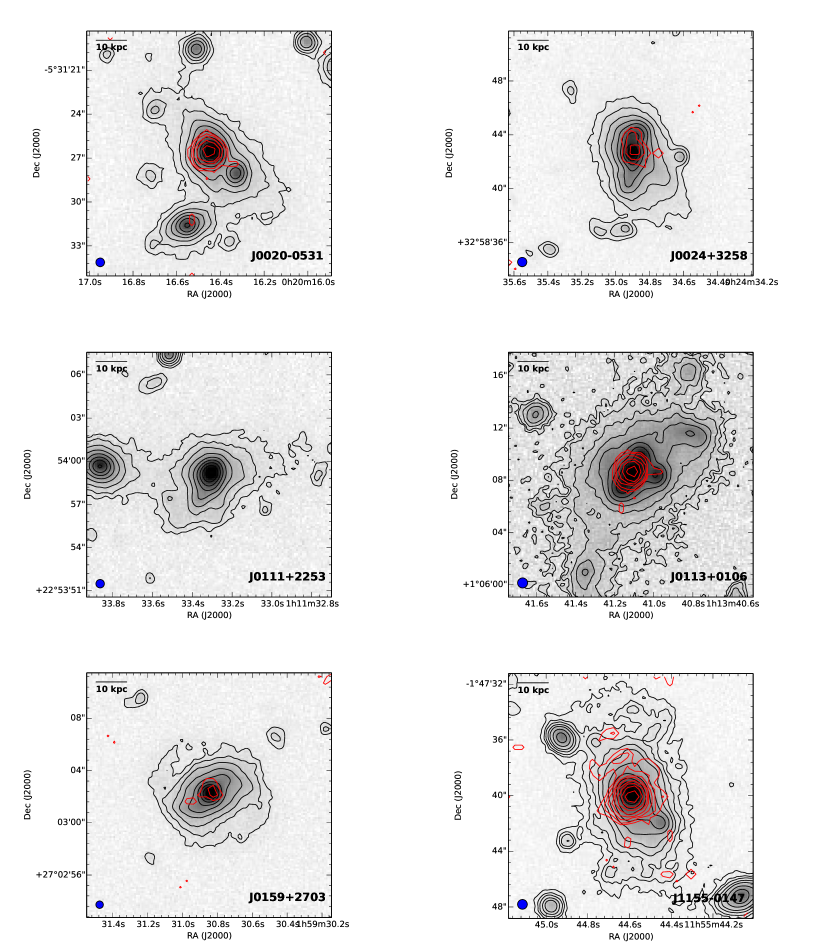
Figure 25: Shown are the $r$-band images of the GBs and the $r$-band contours. A strong non-linear stretch using an asinh() function was applied to the grey-scale image to reveal detail at all brightness levels. The small blue disk at the lower left represents the FWHM of the optical seeing disk. The Chandra X-ray data are shown as red contours if available.

Figure 26: Same as Fig. 25.

Figure 27: Same as Fig. 25.

References

- Allen et al. (2015) Allen J. T., et al., 2015, MNRAS, 451, 2780
- Amorín et al. (2010) Amorín R. O., Pérez-Montero E., Vílchez J. M., 2010, ApJ, 715, L128
- Amorín et al. (2012) Amorín R., Pérez-Montero E., Vílchez J. M., Papaderos P., 2012, ApJ, 749, 185
- Antonucci (1993) Antonucci R., 1993, ARA&A, 31, 473
- Applegate et al. (2014) Applegate D. E., et al., 2014, MNRAS, 439, 48
- Barger et al. (2012) Barger A. J., Cowie L. L., Wold I. G. B., 2012, ApJ, 749, 106
- Bassani et al. (1999) Bassani L., Dadina M., Maiolino R., Salvati M., Risaliti G., Della Ceca R., Matt G., Zamorani G., 1999, ApJS, 121, 473
- Basu-Zych & Scharf (2004) Basu-Zych A., Scharf C., 2004, ApJ, 615, L85
- Bertin (2006) Bertin E., 2006, in Gabriel C., Arviset C., Ponz D., Enrique S., eds, ASP Conf. Ser. Vol. 351, ADASS XV. p. 112
- Binette & Robinson (1987) Binette L., Robinson A., 1987, A&A, 177, 11
- Bournaud et al. (2011) Bournaud F., Dekel A., Teyssier R., Cacciato M., Daddi E., Juneau S., Shankar F., 2011, ApJ, 741, L33
- Bournaud et al. (2012) Bournaud F., et al., 2012, ApJ, 757, 81
- Bridge et al. (2013) Bridge C. R., et al., 2013, ApJ, 769, 91
- Bruzual & Charlot (2003) Bruzual G., Charlot S., 2003, MNRAS, 344, 1000
- Cardamone et al. (2009) Cardamone C., et al., 2009, MNRAS, 399, 1191
- Cen & Zheng (2013) Cen R., Zheng Z., 2013, ApJ, 775, 112
- Chandrasekhar (1943) Chandrasekhar S., 1943, ApJ, 97, 255
- Chapman et al. (2001) Chapman S. C., Lewis G. F., Scott D., Richards E., Borys C., Steidel C. C., Adelberger K. L., Shapley A. E., 2001, ApJ, 548, L17
- Chapman et al. (2004) Chapman S. C., Scott D., Windhorst R. A., Frayer D. T., Borys C., Lewis G. F., Ivison R. J., 2004, ApJ, 606, 85
- Chung et al. (2011) Chung C., Yoon S.-J., Lee Y.-W., 2011, ApJ, 740, L45
- Comerford & Greene (2014) Comerford J. M., Greene J. E., 2014, ApJ, 789, 112
- Comerford et al. (2012) Comerford J. M., Gerke B. F., Stern D., Cooper M. C., Weiner B. J., Newman J. A., Madsen K., Barrows R. S., 2012, ApJ, 753, 42
- Conroy & Gunn (2010) Conroy C., Gunn J. E., 2010, ApJ, 712, 833
- Davies et al. (2015) Davies R. L., Schirmer M., Turner J. E. H., 2015, MNRAS, 449, 1731
- DeGraf et al. (2014) DeGraf C., Dekel A., Gabor J., Bournaud F., 2014, preprint, (arXiv:1412.3819)
- Dey et al. (2005) Dey A., et al., 2005, ApJ, 629, 654
- Dijkstra & Loeb (2009) Dijkstra M., Loeb A., 2009, MNRAS, 400, 1109
- Dijkstra et al. (2006) Dijkstra M., Haiman Z., Spaans M., 2006, ApJ, 649, 14
- Ebeling et al. (2001) Ebeling H., Edge A. C., Henry J. P., 2001, ApJ, 553, 668
- Erb et al. (2011) Erb D. K., Bogosavljević M., Steidel C. C., 2011, ApJ, 740, L31
- Erben et al. (2005) Erben T., Schirmer M., Dietrich J., et al., 2005, AN, 326, 432
- Erben et al. (2013) Erben T., et al., 2013, MNRAS, 433, 2545
- Faucher-Giguère et al. (2010) Faucher-Giguère C.-A., Kereš D., Dijkstra M., Hernquist L., Zaldarriaga M., 2010, ApJ, 725, 633
- Francis et al. (2001) Francis P. J., et al., 2001, ApJ, 554, 1001
- Furlanetto & Lidz (2011) Furlanetto S. R., Lidz A., 2011, ApJ, 735, 117
- Gabor & Bournaud (2014) Gabor J. M., Bournaud F., 2014, MNRAS, 441, 1615
- Geach et al. (2009) Geach J. E., et al., 2009, ApJ, 700, 1
- Goerdt et al. (2010) Goerdt T., Dekel A., Sternberg A., Ceverino D., Teyssier R., Primack J. R., 2010, MNRAS, 407, 613
- Greene et al. (2012) Greene J. E., Zakamska N. L., Smith P. S., 2012, ApJ, 746, 86
- Guainazzi et al. (2005) Guainazzi M., Matt G., Perola G. C., 2005, A&A, 444, 119
- Haiman et al. (2000) Haiman Z., Spaans M., Quataert E., 2000, ApJ, 537, L5
- Hainline et al. (2013) Hainline K. N., Hickox R., Greene J. E., Myers A. D., Zakamska N. L., 2013, ApJ, 774, 145
- Han et al. (2007) Han Z., Podsiadlowski P., Lynas-Gray A. E., 2007, MNRAS, 380, 1098
- Hansen et al. (2005) Hansen S. M., McKay T. A., Wechsler R. H., Annis J., Sheldon E. S., Kimball A., 2005, ApJ, 633, 122
- Hansen et al. (2009) Hansen S. M., Sheldon E. S., Wechsler R. H., Koester B. P., 2009, ApJ, 699, 1333
- Harrison et al. (2014) Harrison C. M., Alexander D. M., Mullaney J. R., Swinbank A. M., 2014, MNRAS, 441, 3306
- Hasinger (2008) Hasinger G., 2008, A&A, 490, 905
- Hawley (2012) Hawley S. A., 2012, PASP, 124, 21
- Hayes et al. (2011) Hayes M., Scarlata C., Siana B., 2011, Nature, 476, 304
- Heckman et al. (2004) Heckman T. M., Kauffmann G., Brinchmann J., Charlot S., Tremonti C., White S. D. M., 2004, ApJ, 613, 109
- Henry et al. (2015) Henry A., Scarlata C., Martin C. L., Erb D., 2015, ApJ, 809, 19
- Herenz et al. (2015) Herenz E. C., Wisotzki L., Roth M., Anders F., 2015, A&A, 576, A115
- Hickox et al. (2014) Hickox R. C., Mullaney J. R., Alexander D. M., Chen C.-T. J., Civano F. M., Goulding A. D., Hainline K. N., 2014, ApJ, 782, 9
- Hildebrandt et al. (2012) Hildebrandt H., et al., 2012, MNRAS, 421, 2355
- Hönig & Kishimoto (2011) Hönig S. F., Kishimoto M., 2011, A&A, 534, A121
- Hopkins & Quataert (2010) Hopkins P. F., Quataert E., 2010, MNRAS, 407, 1529
- Hu (1992) Hu E. M., 1992, ApJ, 391, 608
- Humphrey et al. (2013) Humphrey A., Vernet J., Villar-Martín M., di Serego Alighieri S., Fosbury R. A. E., Cimatti A., 2013, ApJ, 768, L3
- Hunter (2007) Hunter J. D., 2007, Computing In Science & Engineering, 9, 90
- Hutchings (2014) Hutchings J. B., 2014, Ap&SS, 354, 143
- Ichikawa et al. (2012) Ichikawa K., Ueda Y., Terashima Y., Oyabu S., Gandhi P., Matsuta K., Nakagawa T., 2012, ApJ, 754, 45
- Izotov et al. (2011) Izotov Y. I., Guseva N. G., Thuan T. X., 2011, ApJ, 728, 161
- Jaskot & Oey (2013) Jaskot A. E., Oey M. S., 2013, ApJ, 766, 91
- Johnston et al. (2007) Johnston D. E., et al., 2007, astro-ph/0709.1159,
- Keel et al. (2002) Keel W. C., Wu W., Waddington I., Windhorst R. A., Pascarelle S. M., 2002, AJ, 123, 3041
- Keel et al. (2009) Keel W. C., White III R. E., Chapman S., Windhorst R. A., 2009, AJ, 138, 986
- Keel et al. (2012a) Keel W. C., et al., 2012a, AJ, 144, 66
- Keel et al. (2012b) Keel W. C., et al., 2012b, MNRAS, 420, 878
- Keel et al. (2015) Keel W. C., et al., 2015, AJ, 149, 155
- Khrykin et al. (2016) Khrykin I. S., Hennawi J. F., McQuinn M., Worseck G., 2016, ApJ, 824, 133
- Kirkman & Tytler (2008) Kirkman D., Tytler D., 2008, MNRAS, 391, 1457
- Kodaira et al. (2003) Kodaira K., et al., 2003, PASJ, 55, L17
- Kollmeier et al. (2010) Kollmeier J. A., Zheng Z., Davé R., Gould A., Katz N., Miralda-Escudé J., Weinberg D. H., 2010, ApJ, 708, 1048
- Krolik & Kallman (1987) Krolik J. H., Kallman T. R., 1987, ApJ, 320, L5
- Kubo et al. (2015) Kubo M., Yamada T., Ichikawa T., Kajisawa M., Matsuda Y., Tanaka I., 2015, ApJ, 799, 38
- LaMassa et al. (2015) LaMassa S. M., et al., 2015, ApJ, 800, 144
- Lamastra et al. (2009) Lamastra A., Bianchi S., Matt G., Perola G. C., Barcons X., Carrera F. J., 2009, A&A, 504, 73
- Laursen & Sommer-Larsen (2007) Laursen P., Sommer-Larsen J., 2007, ApJ, 657, L69
- Lintott et al. (2009) Lintott C. J., et al., 2009, MNRAS, 399, 129
- Liu et al. (2011) Liu X., Shen Y., Strauss M. A., Hao L., 2011, ApJ, 737, 101
- Liu et al. (2012) Liu X., Shen Y., Strauss M. A., 2012, ApJ, 745, 94
- Liu et al. (2013) Liu G., Zakamska N. L., Greene J. E., Nesvadba N. P. H., Liu X., 2013, MNRAS, 430, 2327
- Lu & Zhou (2005) Lu J.-F., Zhou B.-Y., 2005, ApJ, 635, L17
- Malhotra & Rhoads (2002) Malhotra S., Rhoads J. E., 2002, ApJ, 565, L71
- Malizia et al. (2009) Malizia A., Stephen J. B., Bassani L., Bird A. J., Panessa F., Ubertini P., 2009, MNRAS, 399, 944
- Maraston (2005) Maraston C., 2005, MNRAS, 362, 799
- Maraston et al. (2009) Maraston C., Nieves Colmenárez L., Bender R., Thomas D., 2009, A&A, 493, 425
- Martin et al. (2014) Martin D. C., Chang D., Matuszewski M., Morrissey P., Rahman S., Moore A., Steidel C. C., Matsuda Y., 2014, ApJ, 786, 107
- Mateus et al. (2006) Mateus A., Sodré L., Cid Fernandes R., Stasińska G., Schoenell W., Gomes J. M., 2006, MNRAS, 370, 721
- Matsuda et al. (2004) Matsuda Y., et al., 2004, AJ, 128, 569
- Matsuda et al. (2006) Matsuda Y., Yamada T., Hayashino T., Yamauchi R., Nakamura Y., 2006, ApJ, 640, L123
- Matsuda et al. (2011) Matsuda Y., et al., 2011, MNRAS, 410, L13
- McDonald et al. (2012) McDonald M., et al., 2012, Nature, 488, 349
- McDonald et al. (2015) McDonald M., et al., 2015, ApJ, 811, 111
- McLinden et al. (2011) McLinden E. M., et al., 2011, ApJ, 730, 136
- McLinden et al. (2014) McLinden E. M., Rhoads J. E., Malhotra S., Finkelstein S. L., Richardson M. L. A., Smith B., Tilvi V. S., 2014, MNRAS, 439, 446
- Meinköhn & Richling (2002) Meinköhn E., Richling S., 2002, A&A, 392, 827
- Merloni et al. (2014) Merloni A., et al., 2014, MNRAS, 437, 3550
- Miyaji et al. (2015) Miyaji T., et al., 2015, ApJ, 804, 104
- Mullaney et al. (2013) Mullaney J. R., Alexander D. M., Fine S., Goulding A. D., Harrison C. M., Hickox R. C., 2013, MNRAS, 433, 622
- Nenkova et al. (2008) Nenkova M., Sirocky M. M., Ivezić Ž., Elitzur M., 2008, ApJ, 685, 147
- Neufeld (1990) Neufeld D. A., 1990, ApJ, 350, 216
- Nilsson et al. (2006) Nilsson K. K., Fynbo J. P. U., Møller P., Sommer-Larsen J., Ledoux C., 2006, A&A, 452, L23
- Novak et al. (2011) Novak G. S., Ostriker J. P., Ciotti L., 2011, ApJ, 737, 26
- Nussbaumer & Schmutz (1984) Nussbaumer H., Schmutz W., 1984, A&A, 138, 495
- Nusser & Sheth (1999) Nusser A., Sheth R. K., 1999, MNRAS, 303, 685
- O’Connell (1999) O’Connell R. W., 1999, ARA&A, 37, 603
- O’Dea et al. (2004) O’Dea C. P., Baum S. A., Mack J., Koekemoer A. M., Laor A., 2004, ApJ, 612, 131
- O’Dea et al. (2010) O’Dea K. P., et al., 2010, ApJ, 719, 1619
- Osterbrock & Ferland (2006) Osterbrock D. E., Ferland G. J., 2006, Astrophysics of gaseous nebulae and active galactic nuclei. University Science Books
- Ouchi et al. (2009) Ouchi M., et al., 2009, ApJ, 696, 1164
- Overzier et al. (2013) Overzier R. A., Nesvadba N. P. H., Dijkstra M., Hatch N. A., Lehnert M. D., Villar-Martín M., Wilman R. J., Zirm A. W., 2013, ApJ, 771, 89
- Palunas et al. (2004) Palunas P., Teplitz H. I., Francis P. J., Williger G. M., Woodgate B. E., 2004, ApJ, 602, 545
- Pengelly & Seaton (1964) Pengelly R. M., Seaton M. J., 1964, MNRAS, 127, 165
- Pilyugin et al. (2012) Pilyugin L. S., Vílchez J. M., Mattsson L., Thuan T. X., 2012, MNRAS, 421, 1624
- Pogge & De Robertis (1993) Pogge R. W., De Robertis M. M., 1993, ApJ, 404, 563
- Prescott et al. (2008) Prescott M. K. M., Kashikawa N., Dey A., Matsuda Y., 2008, ApJ, 678, L77
- Prescott et al. (2012) Prescott M. K. M., Dey A., Jannuzi B. T., 2012, ApJ, 748, 125
- Prescott et al. (2013) Prescott M. K. M., Dey A., Jannuzi B. T., 2013, ApJ, 762, 38
- Prescott et al. (2015) Prescott M. K. M., Momcheva I., Brammer G. B., Fynbo J. P. U., Møller P., 2015, ApJ, 802, 32
- Rampadarath et al. (2010) Rampadarath H., et al., 2010, A&A, 517, L8
- Ree et al. (2012) Ree C. H., Jeong H., Oh K., Chung C., Lee J. H., Kim S. C., Kyeong J., 2012, ApJ, 744, L10
- Rengstorf et al. (2004) Rengstorf A. W., et al., 2004, ApJ, 617, 184
- Reyes et al. (2008) Reyes R., et al., 2008, AJ, 136, 2373
- Risaliti et al. (1999) Risaliti G., Maiolino R., Salvati M., 1999, ApJ, 522, 157
- Rosdahl & Blaizot (2012) Rosdahl J., Blaizot J., 2012, MNRAS, 423, 344
- Ross et al. (2013) Ross N. P., et al., 2013, ApJ, 773, 14
- Roy et al. (2010) Roy I., Shu C.-W., Fang L.-Z., 2010, ApJ, 716, 604
- Runnoe et al. (2016) Runnoe J. C., et al., 2016, MNRAS, 455, 1691
- Saito et al. (2006) Saito T., Shimasaku K., Okamura S., Ouchi M., Akiyama M., Yoshida M., 2006, ApJ, 648, 54
- Saito et al. (2008) Saito T., Shimasaku K., Okamura S., Ouchi M., Akiyama M., Yoshida M., Ueda Y., 2008, ApJ, 675, 1076
- Schawinski et al. (2010) Schawinski K., et al., 2010, ApJ, 724, L30
- Schawinski et al. (2015) Schawinski K., Koss M., Berney S., Sartori L. F., 2015, MNRAS, 451, 2517
- Schirmer (2013) Schirmer M., 2013, ApJS, 209, 21
- Schirmer et al. (2011) Schirmer M., Hildebrandt H., Kuijken K., Erben T., 2011, A&A, 532, 57
- Schirmer et al. (2013) Schirmer M., Diaz R., Holhjem K., Levenson N. A., Winge C., 2013, ApJ, 763, 60
- Schlafly & Finkbeiner (2011) Schlafly E. F., Finkbeiner D. P., 2011, ApJ, 737, 103
- Schweizer et al. (2013) Schweizer F., Seitzer P., Kelson D. D., Villanueva E. V., Walth G. L., 2013, ApJ, 773, 148
- Shen et al. (2011) Shen Y., Liu X., Greene J. E., Strauss M. A., 2011, ApJ, 735, 48
- Sijacki et al. (2015) Sijacki D., Vogelsberger M., Genel S., Springel V., Torrey P., Snyder G. F., Nelson D., Hernquist L., 2015, MNRAS, 452, 575
- Silk (2013) Silk J., 2013, ApJ, 772, 112
- Silk et al. (2013) Silk J., Di Cintio A., Dvorkin I., 2013, preprint, (arXiv:1312.0107)
- Snyder (1998) Snyder J. A., 1998, in D’Odorico S., ed., Society of Photo-Optical Instrumentation Engineers (SPIE) Conference Series Vol. 3355, Optical Astronomical Instrumentation. pp 635–645
- Steidel et al. (1995) Steidel C. C., Pettini M., Hamilton D., 1995, AJ, 110, 2519
- Steidel et al. (2000) Steidel C. C., Adelberger K. L., Shapley A. E., Pettini M., Dickinson M., Giavalisco M., 2000, ApJ, 532, 170
- Steidel et al. (2011) Steidel C. C., Bogosavljević M., Shapley A. E., Kollmeier J. A., Reddy N. A., Erb D. K., Pettini M., 2011, ApJ, 736, 160
- Stern et al. (2014) Stern D., et al., 2014, ApJ, 794, 102
- Swinbank et al. (2015) Swinbank A. M., et al., 2015, MNRAS, 449, 1298
- Tamura et al. (2013) Tamura Y., et al., 2013, MNRAS, 430, 2768
- Taniguchi & Shioya (2000) Taniguchi Y., Shioya Y., 2000, ApJ, 532, L13
- Tokovinin et al. (2010) Tokovinin A., et al., 2010, in Society of Photo-Optical Instrumentation Engineers (SPIE) Conference Series. p. 3, doi:10.1117/12.856407
- Tokovinin et al. (2012) Tokovinin A., Tighe R., Schurter P., Cantarutti R., van der Bliek N., Martinez M., Mondaca E., Heathcote S., 2012, in Society of Photo-Optical Instrumentation Engineers (SPIE) Conference Series. p. 4, doi:10.1117/12.925705
- Trebitsch et al. (2014) Trebitsch M., Verhamme A., Blaizot J., Rosdahl J., 2014, in Ballet J., Martins F., Bournaud F., Monier R., Reylé C., eds, SF2A-2014: Proceedings of the Annual meeting of the French Society of Astronomy and Astrophysics. pp 375–377
- Ueda et al. (2014) Ueda Y., Akiyama M., Hasinger G., Miyaji T., Watson M. G., 2014, ApJ, 786, 104
- Verhamme et al. (2006) Verhamme A., Schaerer D., Maselli A., 2006, A&A, 460, 397
- Webb et al. (2009) Webb T. M. A., Yamada T., Huang J.-S., Ashby M. L. N., Matsuda Y., Egami E., Gonzalez M., Hayashimo T., 2009, ApJ, 692, 1561
- Weijmans et al. (2010) Weijmans A.-M., Bower R. G., Geach J. E., Swinbank A. M., Wilman R. J., de Zeeuw P. T., Morris S. L., 2010, MNRAS, 402, 2245
- White et al. (1997) White R. L., Becker R. H., Helfand D. J., Gregg M. D., 1997, ApJ, 475, 479
- Williamson et al. (2011) Williamson R., et al., 2011, ApJ, 738, 139
- Wold et al. (2014) Wold I. G. B., Barger A. J., Cowie L. L., 2014, ApJ, 783, 119
- Xu et al. (2011) Xu W., Wu X.-P., Fang L.-Z., 2011, MNRAS, 418, 853
- Yajima et al. (2013) Yajima H., Li Y., Zhu Q., 2013, ApJ, 773, 151
- Yang et al. (2009) Yang Y., Zabludoff A., Tremonti C., Eisenstein D., Davé R., 2009, ApJ, 693, 1579
- Yang et al. (2010) Yang Y., Zabludoff A., Eisenstein D., Davé R., 2010, ApJ, 719, 1654
- Yang et al. (2011a) Yang Y., Zabludoff A., Jahnke K., Eisenstein D., Davé R., Shectman S. A., Kelson D. D., 2011a, ApJ, 735, 87
- Yang et al. (2011b) Yang Y., Roy I., Shu C.-W., Fang L.-Z., 2011b, ApJ, 739, 91
- Yang et al. (2014) Yang Y., Zabludoff A., Jahnke K., Davé R., 2014, ApJ, 793, 114
- Yang et al. (2015) Yang H., Malhotra S., Gronke M., Rhoads J. E., Jaskot A., Zheng Z., Dijkstra M., 2015, preprint, (arXiv:1506.02885)
- Zabl et al. (2015) Zabl J., Nørgaard-Nielsen H. U., Fynbo J. P. U., Laursen P., Ouchi M., Kjærgaard P., 2015, preprint, (arXiv:1505.01859)
- Zakamska et al. (2005) Zakamska N. L., et al., 2005, AJ, 129, 1212