Abstract

Spline Galerkin methods for the double layer potential equation on contours with corners are studied. The stability of the method depends on the invertibility of some operators $R_{\tau}$ associated with the corner points $\tau$. The operators $R_{\tau}$ do not depend on the shape of the contour but only on the opening angles of the corner points $\tau$. The invertibility of these operators is studied numerically via the stability of the method on model curves, all corner points of which have the same opening angle. The case of the splines of order $0,1$ and $2$ is considered. It is shown that no opening angle located in the interval $[0.1\pi,1.9\pi]$ can cause the instability of the method. This result is in strong contrast with the Nyström method, which has four instability angles in the interval mentioned. Numerical experiments show a good convergence of the methods even if the right-hand side of the equation has discontinuities located at the corner points of the contour.

2010 Mathematics Subject Classification: Primary 45L05; Secondary 65R20

Key Words: Double layer potential equation, spline Galerkin method, critical angle

1 Introduction

Let $D$ be a simply connected bounded domain in ${\mathbb{R}}^{2}$ with boundary $\Gamma$, and let $n_{\tau}$ denote the outer normal to $\Gamma$ at the point $\tau\in\Gamma$. It is well known that the solution of various boundary value problems for the Laplace equation can be reduced to solution of the integral equation

$$(A_{\Gamma}\omega)(t)=\omega(t)+\frac{1}{\pi}\int_{\Gamma}\omega(\tau)\frac{d}{dn_{\tau}}\log|t-\tau|\,ds_{\tau}+(T\omega)(t)=f(t),\quad t=x+iy\in\Gamma$$ (1)

where $ds_{\tau}$ refer to the arc length differential and $T$ is a compact operator. The operator

$$V_{\Gamma}\omega(t):=\frac{1}{\pi}\int_{\Gamma}\omega(\tau)\frac{d}{dn_{\tau}}\log|t-\tau|\,ds_{\tau}$$

is called the double layer potential operator and it is well known [23] that it can be represented in the form

$$V_{\Gamma}=\frac{1}{2}(S_{\Gamma}+MS_{\Gamma}M),$$

where $S_{\Gamma}$ is the Cauchy singular integral operator on $\Gamma$,

$$(S_{\Gamma}x)(t):=\frac{1}{\pi i}\int_{\Gamma}\frac{x(\tau)\,d\tau}{\tau-t}.$$

and $M$ is the operator of complex conjugation, $M\varphi(t):=\overline{\varphi(t)}$.

If $\Gamma$ is a smooth closed curve, then the double layer potential operator $V_{\Gamma}$ is compact in the space $L^{p}$. This fact essentially simplifies the stability investigation of approximation methods for the equation (1). However, if $\Gamma$ possesses corner points, the situation becomes more involved. One of the simplest cases to treat is a polygonal boundary or a boundary with polygonally shaped corners and there are a number of works investigating approximation methods for the equation (1) on such curves [3, 5, 6, 16, 19, 21]. For a comprehensive survey, we refer the reader to [2, 20].

In the present work we consider spline Galerkin methods for the double layer potential equation (1) in the case of simple piecewise smooth curves. Such methods are often used to determine approximate solutions of (1). However, for contours with corners, the stability analysis of the methods is not complete. On the other hand, it is known that for boundary integral equations the presence of corners on the boundary may lead to extra conditions required for the stability of the approximation method considered [9, 10, 11, 13]. The aim of the present work is twofold. First, we obtain necessary and sufficient conditions for the stability of spline Galerkin methods. It turns out that stability depends on the invertibility of some operators associated with corner points of $\Gamma$. These operators belong to an algebra of Toeplitz operators and, at present, there is no tool to verify their invertibility. Therefore, our second goal is to present an approach to check the invertibility of the operators mentioned. This approach is based on considering our approximation methods on special model curves, and it allows us to show that Galerkin methods for double layer potential equations on piecewise smooth contours behave similarly to equations on smooth curves. Thus, it was discovered that at least for the splines of degree $0,1$ and $2$ the corresponding Galerkin method is always stable provided that all opening angles of the corner points are located in the interval $[0.1\pi,1.9\pi]$. Similar results concerning the spline Galerkin methods for the Sherman-Lauricella equation have been recently obtained in [12]. Note that this effect is in strong contrast with the behaviour of the Nyström method which possesses instability angles in the interval $[0.1\pi,1.9\pi]$, [13].

This paper is organized as follows. Section 2 is devoted to description of spline spaces and spline Galerkin methods. Here we also present some numerical examples illustrating the efficiency of the method. Stability conditions are established in Section 3, while Section 4 deals with the numerical approach to the search of critical angles.

2 Spline spaces and spline Galerkin methods

Let us identify each point $(x,y)$ of ${\mathbb{R}}^{2}$ with the corresponding point $z=x+iy$ in the complex plane ${\mathbb{C}}$. By $L^{2}=L^{2}(\Gamma)$ we denote the set of all Lebesgue measurable functions $f=f(t),t\in\Gamma$ such that

$$||f||=\left(\int_{\Gamma}|f(t)|^{2}\,|dt|\right)^{1/2}<+\infty.$$

By $\mathcal{M}_{\Gamma}$ we denote the set of all corner points $\tau_{0},\tau_{1},\ldots,\tau_{q-1}$ of $\Gamma$. In order to describe the spline spaces on $\Gamma$, let us assume that this contour is parametrized by a $1$-periodic function $\gamma:{\mathbb{R}}\mapsto{\mathbb{C}}$ such that

$$\tau_{k}=\gamma\left(\frac{k}{q}\right),\;k=0,1,\ldots,q-1.$$ (2)

In addition, we also assume that the function $\gamma$ is two times continuously differentiable on each subinterval $(k/q,(k+1)/q)$ and

$$\left|\gamma^{\prime}\left(\frac{k}{q}+0\right)\right|=\left|\gamma^{\prime}\left(\frac{k}{q}-0\right)\right|,\;k=0,1,\ldots,q-1.$$ (3)

For any two functions $f,g\in L^{2}({\mathbb{R}})$, let $f*g$ denote their convolution, i.e.

$$(f*g)(s):=\int\limits_{{\mathbb{R}}}f(s-x)g(x)dx.$$

If $\chi$ is the characteristic function of the interval $[0,1)$, then for any fixed $d\in{\mathbb{N}}$, let $\widehat{\phi}=\widehat{\phi}^{(d)}(s)$ be the function defined by the recursive relation

$$\widehat{\phi}^{(d)}(s)=\begin{cases}\chi(s)&\text{ if }d=0,\\ (\chi*\widehat{\phi}^{(d-1)})(s)&\text{ if }d>0.\end{cases}$$

The parametrization $\gamma$ can be now used to introduce spline spaces on $\Gamma$. More precisely, let $n$ and $d$ be fixed non-negative integers such that $n\geqslant d+1$. By $\mathcal{I}(n,d)$ we denote the set of all integers $j\in\{0,1,\ldots,n-(d+1)\}$ such that the interval $[j/n,(j+d+1)/n]$ does not contain any point $s_{k}=k/q$, $k=0,1,\ldots,q$. Let $S^{d}_{n}=S^{d}_{n}(\Gamma)$ be the set of all linear combinations of the functions

$$\widehat{\phi}_{nj}(t)=\widehat{\phi}^{(d)}(ns-j),\;t=\gamma(s)\in\Gamma,\quad s\in{\mathbb{R}},\quad j\in\mathcal{I}(n,d).$$

For each $j\in\mathcal{I}(n,d)$ set

$$\phi_{nj}:=\nu_{d}\sqrt{n}\widehat{\phi}_{nj},$$

where

$$\nu_{d}=\left(\int\limits_{0}^{d+1}\left|\widehat{\phi}^{(d)}(s)\right|^{2}ds\right)^{-1/2}.$$

It is easily seen that $\phi_{nj}$ are normalized functions, i.e. $||\phi_{nj}||=1$.

According to the spline Galerkin method, approximate solution $\omega_{n}$ of the equation (1) is sought in the form

$$\omega_{n}(t)=\sum\limits_{j\in\mathcal{I}(n,d)}a_{j}\phi_{nj}(t)$$ (4)

with the coefficients $a_{j}$ obtained from the system of linear algebraic equations

$$(A_{\Gamma}\omega_{n},\phi_{nj})=(f,\phi_{nj}),\quad j\in\mathcal{I}(n,d).$$ (5)

Note that the scalar product $(\cdot,\cdot)$ is defined by

$$(f,g)=\int\limits_{0}^{1}f(\gamma(s))\overline{g(\gamma(s))}ds.$$

The stability of this Galerkin method will be studied in Section 3. However, here we would like to illustrate the efficiency of the method by a few examples. For simplicity, now we only consider equations with the operator $T=0$. Although special, this case is of the utmost importance. It occurs when reducing boundary value problems for partial differential equations to boundary integral equations. In particular, we determine Galerkin solutions of the double layer potential equation with various right-hand sides $f$ on two curves with corners. One of these right-hand sides is continuous on both curves, whereas two others have discontinuity points, some of which coincide with the corners. Let us describe the curves and right-hand sides in more details. The curves ${\mathfrak{L}}$ and ${\mathfrak{M}}$ are obtained from the ellipse

$$\gamma_{e}(s)=a\cos(2\pi s)+ib\sin(2\pi s),\quad s\in{\mathbb{R}},$$

by cutting a part of it and connecting the cutting points by arcs representing cubic Hermit interpolation polynomials in such a way that each common point of the curve obtained becomes a corner point satisfying the conditions (2), (3). In Figure 1, the semi-axes of the ellipse are $a=3,b=4$. The curve ${\mathfrak{L}}$ has two corner points obtained by cutting off the part of the ellipse corresponding to the parameter $s\in[3/8,5/8]$. On the other hand, two parts of the ellipse corresponding to the parameter $s\in[3/8,5/8]\cup[7/8,9/8]$ are cut off to create the curve ${\mathfrak{M}}$. The parametrization of the remaining parts of the curves ${\mathfrak{L}}$ and ${\mathfrak{M}}$ is scaled and shifted so that the conditions (2) and (3) are satisfied. Let $f_{1},f_{2}$ and $f_{3}$ be the following functions defined on the curves ${\mathfrak{L}}$ and ${\mathfrak{M}}$,

$$f_{1}(z)=-z|z|,$$

$$f_{2}(z)=\begin{cases}-1+iz&\text{ if }\textrm{Im}\,z<0,\\ \quad\!1+iz&\text{ if }\textrm{Im}\,z\geqslant 0,\end{cases}$$

and

$$f_{3}(z)=\begin{cases}-2+iz&\text{ if }\textrm{Im}\,z<\textrm{Im}\,z_{0},\\ \quad\!2+iz&\text{ if }\textrm{Im}\,z\geqslant\textrm{Im}\,z_{0},\end{cases}$$

where $z_{0}=\gamma_{e}(3/8)$.

In passing note that the function $f_{2}$ has two discontinuity points neither of which coincides with a corner of ${\mathfrak{L}}$ or ${\mathfrak{M}}$. On the other hand, one of the corner points of ${\mathfrak{L}}$ is a discontinuity point for the function $f_{3}$, and two discontinuity points of $f_{3}$ are located at the corner points of ${\mathfrak{M}}$. Let $\omega_{n}=\omega_{n}(f_{j},\Gamma)$ be the Galerkin solution (4), (5) of the double layer potential equation with right-hand side $f_{j}$ considered on a curve $\Gamma$, and let $E_{n}^{f_{j},\Gamma}$ be the quantity

$$E_{n}^{f_{j},\Gamma}=\|\omega_{2n}(f_{j},\Gamma)-\omega_{n}(f_{j},\Gamma)\|_{2}/\|\omega_{2n}(f_{j},\Gamma)\|_{2},$$

which shows the rate of convergence of the approximation method under consideration. The Table 1 illustrates how the spline Galerkin method with $d=0$ performs for the curves ${\mathfrak{L}}$ and ${\mathfrak{M}}$ and for the right-hand sides $f_{1},f_{2}$ and $f_{3}$.

Note that the integrals in the scalar products $(A_{\Gamma}\omega_{n},\phi_{nj}),\;j\in\mathcal{I}(n,d)$ are approximated by the Gauss-Legendre quadrature formula with quadrature points coinciding with the zeros of the Legendre polynomial of degree $24$ on the canonical interval $[-1,1]$ scaled and shifted to the intervals $[j/n,(j+d+1)/n]$. More precisely, we employ the formula

$$(A_{\Gamma}\omega_{n},\phi_{nj})=\int\limits_{0}^{1}A_{\Gamma}\omega_{n}(\gamma(s))\overline{\phi_{nj}(\gamma(s))}ds\approx\sum\limits_{k=1}^{24}w_{k}A_{\Gamma}\omega_{n}(\gamma(s_{k}))\phi_{nj}(\gamma(s_{k})),$$ (6)

where $w_{k},s_{k}$ are weights and Gauss-Legendre points on the interval $[j/n,(j+d+1)/n]$. Composite Gauss-Legendre quadrature is also used in approximation of the integral operators of $A_{\Gamma}\omega_{n}(\gamma(s_{k}))$, cf. [9]. Thus we employ the quadrature formula

$$\int_{\Gamma}k(t,\tau)x(\tau)d\tau =\int\limits_{0}^{1}k(\gamma(\sigma),\gamma(s))x(\gamma(s))\gamma^{\prime}(s)ds$$

$$\approx\sum\limits_{l=0}^{m-1}\sum\limits_{p=0}^{r-1}w_{p}k(\gamma(\sigma),\gamma(s_{lp}))x(\gamma(s_{lp}))\gamma^{\prime}(s_{lp})/m$$

where $m=40$, $r=24$, $s_{lp}=(l+\varepsilon_{p})/m$ and $w_{p}$ and $\varepsilon_{p}$ are, respectively, the Gauss-Legendre weights and Gauss-Legendre nodes scaled and shifted to the interval $[0,1]$. For the discrete norm used in error evaluation, we set $h_{0}=1/128$, $h=10^{-3}$ and choose the meshes

$$U_{1}:=(0+h_{0}:h:0.5-h_{0})\bigcup(0.5+h_{0}:h:1-h_{0})$$

and

$$U_{2}:= (0\!+\!h_{0}:h:0.25\!-\!h_{0})\bigcup(0.25\!+\!h_{0}:h:0.5\!-\!h_{0})$$

$$\bigcup(0.5+h_{0}:h:0.75-h_{0})\bigcup(0.75+h_{0}:h:1-h_{0})$$

due to the fact that the curves ${\mathfrak{L}}$ and ${\mathfrak{M}}$ have two and four corner points, respectively, cf. Condition 2. In the graphs of Figure 2, jumps appear when the corner points of ${\mathfrak{M}}$ and the discontinuity points of the right-hand side $f_{3}$ coincide. At the same time, it is quite remarkable that the condition numbers of the methods are relatively small. For the interval considered, they do not exceed $10$ and $5$ for the curve ${\mathfrak{L}}$ and ${\mathfrak{M}}$, respectively.

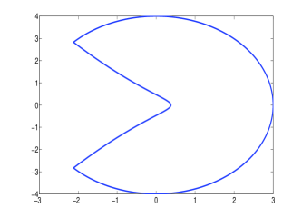
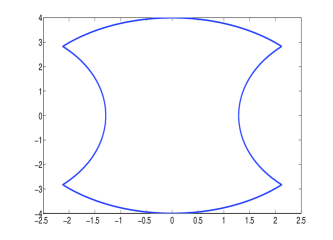
Figure 1: Left: ’pacman’ curve ${\mathfrak{L}}$; Right: ’battleax’ curve ${\mathfrak{M}}$.

n	$E_{n}^{(f_{1},{\mathfrak{L}})}$	$E_{n}^{(f_{1},{\mathfrak{M}})}$	$E_{n}^{(f_{2},{\mathfrak{L}})}$	$E_{n}^{(f_{2},{\mathfrak{M}})}$	$E_{n}^{(f_{3},{\mathfrak{L}})}$	$E_{n}^{(f_{3},{\mathfrak{M}})}$
$128$	$0.0257$	$0.0279$	$0.0248$	$0.0261$	$0.0445$	$0.0383$
$256$	$0.0129$	$0.0147$	$0.0125$	$0.0141$	$0.0286$	$0.0230$
$512$	$0.0054$	$0.0073$	$0.0052$	$0.0070$	$0.0186$	$0.0153$

Table 1: Convergence of the spline Galerkin method, $d=0$.

Let us also point out that the results presented in Table 1 are comparable with the convergence rates of the spline Galerkin methods for the Sherman-Lauricella [22] and Muskhelishvili [14] equations on smooth curves. These estimates can still be improved if one uses a more accurate approximation of the integrals arising in the Galerkin method [17, 18]. Nevertheless, the approximate solutions presented in Figure 2 demonstrate a good accuracy. We also computed Galerkin method solutions of the double layer potential equation with the right-hand sides and curves from [13]. Although these results are not reported here, there is a good correlation with approximate solutions of [13] obtained by the Nyström method.

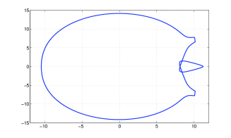
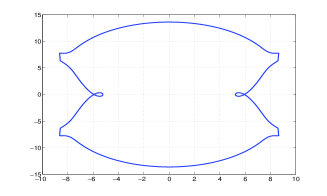
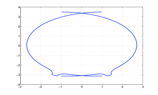
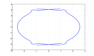
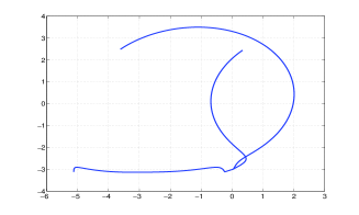
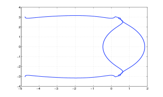
Figure 2: Spline Galerkin solution of the double layer potential equation in the case $n=1024$. Left: ’pacman’ curve ${\mathfrak{L}}$; Right: ’battleax’ curve ${\mathfrak{M}}$. First row: with r.-h. s. $f_{1}(z)$; Second row: with r.-h. s. $f_{2}(z)$; Third row: with r.-h. s.$f_{3}(z)$.

3 Local operators and stability of the spline Galerkin method

Let us briefly describe the approach we use in the study of the stability of the Galerkin method. For more details, we refer the reader to [8, 24, 25]. Let $P_{n}$ denote the orthogonal projection from $L^{2}(\Gamma)$ onto $S_{n}^{d}(\Gamma)$. The spline Galerkin method (5) can be rewritten as

$$P_{n}A_{\Gamma}P_{n}\omega_{n}=P_{n}f,\;n\in{\mathbb{N}}.$$ (7)

Definition 3.1

The approximation sequence $(P_{n}A_{\Gamma}P_{n})$ is said to be stable if there exists $n_{0}\in{\mathbb{N}}$ and a constant $C>0$ such that for all $n\geqslant n_{0}$ the operators $P_{n}A_{\Gamma}P_{n}:S^{d}_{n}(\Gamma)\mapsto S^{d}_{n}(\Gamma)$ are invertible and $\|(P_{n}A_{\Gamma}P_{n})^{-1}P_{n}\|\leqslant C$.

Let $\mathcal{A}^{\Gamma}$ denote the set of all bounded sequences of bounded linear operator $A_{n}:\mathrm{Im}\,P_{n}\mapsto\mathrm{Im}\,P_{n}$ such that there exist strong limits

$$s-\lim A_{n}P_{n}=A,\quad s-\lim(A_{n}P_{n})^{*}P_{n}=A^{*}.$$

Moreover, let $\mathcal{K}(L^{2}(\Gamma))$ denote the ideal of all compact operators in $\mathcal{L}(L^{2}(\Gamma))$, and let $\mathcal{G}\subset\mathcal{A}^{\Gamma}$ be the set of sequences which converge uniformly to zero. Recall that the sequence of orthogonal projection $(P_{n})$ in $L^{2}(\Gamma)$ converges strongly to identity operator and $P_{n}^{*}=P_{n}$. It follows that

$$s-\lim\limits_{n\to\infty}P_{n}A_{\Gamma}P_{n}=A_{\Gamma},\quad s-\lim\limits_{n\to\infty}(P_{n}A_{\Gamma}P_{n})^{*}P_{n}=A^{*}_{\Gamma}.$$

It is well known[8, 24, 25] that the set of sequences

$$\mathcal{J}^{\Gamma}=\{(A_{n})\in\mathcal{A}^{\Gamma}:A_{n}=P_{n}KP_{n}+G_{n},\;K\in\mathcal{K}(L^{2}(\Gamma)),\;(G_{n})\in\mathcal{G}\}$$

forms a close two-sided ideal of $\mathcal{A}^{\Gamma}$.

Proposition 3.1 (cf. [8, Proposition 1.6.4])

The sequence $(P_{n}A_{\Gamma}P_{n})$ is stable if and only if the operator $A_{\Gamma}\in\mathcal{L}(L^{2}(\Gamma))$ and the coset $(P_{n}A_{\Gamma}P_{n})+\mathcal{J}^{\Gamma}\in\mathcal{L}(\mathcal{A}^{\Gamma}/\mathcal{J}^{\Gamma})$ are invertible.

Recall that both Fredholm properties and invertibility of the operator $A_{\Gamma}$ in various spaces have been studied in literature [2, 4, 23, 27]. Therefore, our main task here is to investigate the behaviour of the coset $(P_{n}A_{\Gamma}P_{n})+\mathcal{J}^{\Gamma}$. Note that it is more convenient to consider this coset as an element of a smaller algebra.

Thus let $\mathcal{B}^{\Gamma}$ denote the smallest closed $C^{*}$-subalgebra of $\mathcal{A}^{\Gamma}$ which contains the sequences $(P_{n}MS_{\Gamma}MP_{n}),(P_{n}S_{\Gamma}P_{n})$, all sequences $(G_{n})\in\mathcal{G}$, and all sequences $(P_{n}fP_{n})$ with $f\in C_{{\mathbb{R}}}(\Gamma)$. It follows from [24, 25] that $\mathcal{J}^{\Gamma}\subset\mathcal{B}^{\Gamma}$ and $(P_{n}A_{\Gamma}P_{n})\in\mathcal{B}^{\Gamma}$. Therefore, $\mathcal{B}^{\Gamma}/\mathcal{J}^{\Gamma}$ is a $C^{*}$-subalgebra of $\mathcal{A}^{\Gamma}/\mathcal{J}^{\Gamma}$, hence the coset $(P_{n}A_{\Gamma}P_{n})+\mathcal{J}^{\Gamma}$ is invertible in $\mathcal{A}^{\Gamma}/\mathcal{J}^{\Gamma}$ if and only if it is invertible in $\mathcal{B}^{\Gamma}/\mathcal{J}^{\Gamma}$. However, the invertibility of the coset $(P_{n}A_{\Gamma}P_{n})+\mathcal{J}^{\Gamma}$ in the quotient algebra $\mathcal{B}^{\Gamma}/\mathcal{J}^{\Gamma}$ can be showed by a local principle. Thus, with each point $\tau\in\Gamma$, we associate a curve $\Gamma_{\tau}$ as follows. Let $\theta_{\tau}\in(0,2\pi)$ be the angle between the right and left semi-tangents to $\Gamma$ at the point $\tau$. Further, let $\beta_{\tau}\in(0,2\pi)$ be the angle between the real axis ${\mathbb{R}}$ and the right semi-tangent to $\Gamma$ at the same point $\tau$. Let $\Gamma_{\tau}$ be the curve defined by

$${\Gamma_{\tau}}:=e^{i(\beta_{\tau}+\theta_{\tau})}{\mathbb{R}}^{+}_{-}\,\bigcup\,e^{i\beta_{\tau}}{\mathbb{R}}_{+}^{+}$$

where ${\mathbb{R}}^{+}_{-}$ and ${\mathbb{R}}_{+}^{+}$ are positive semi-axes directed to and away from zero, respectively. On the curve $\Gamma_{\tau}$ consider the corresponding double layer potential operator $A_{\Gamma_{\tau}}=I+V_{\Gamma_{\tau}}$. Moreover, let

$$\widetilde{\phi}_{nj}(t)=\begin{cases}\begin{cases}\widehat{\phi}^{(d)}(ns-j)&\text{ if }t=e^{i\beta_{\tau}}s\\ 0&\text{ otherwise }\end{cases}\quad j\geqslant 0,\\ \begin{cases}\widehat{\phi}^{(d)}(ns-j+d)&\text{ if }t=e^{i(\beta_{\tau}+\theta_{\tau})}s\\ 0&\text{ otherwise }\end{cases}\quad j<0\\ \end{cases}.$$

By $S_{n}^{d}({\Gamma_{\tau}})$ we denote the smallest closed subspace of $L^{2}({\Gamma_{\tau}})$ which contains all functions $\widetilde{\phi}_{nj}$, $j\in{\mathbb{Z}}$. Correspondingly, $S_{n}^{d}({\mathbb{R}}^{+})$ is the smallest subspace of $L^{2}({\mathbb{R}}^{+})$ containing all functions $\widetilde{\phi}_{nj}$, $j\geqslant 0$ for $\beta_{\tau}=0$. In addition, let $P_{n}^{\tau}$ and $P_{n}^{+}$ be the orthogonal projections of $L^{2}({\Gamma_{\tau}})$ onto $S_{n}^{d}({\Gamma_{\tau}})$ and $L^{2}({\mathbb{R}}^{+})$ onto $S_{n}^{d}({\mathbb{R}}^{+})$, respectively. Now algebra $\mathcal{B}^{\Gamma_{\tau}}$ and its ideal $\mathcal{J}^{\Gamma_{\tau}}$ can be defined analogously to the construction of $\mathcal{B}^{\Gamma}$ and $\mathcal{J}^{\Gamma}$.

Similarly to Proposition 3.1, one can formulate the following result.

Lemma 3.1

The sequence $(P_{n}^{\tau}A_{\Gamma_{\tau}}P_{n}^{\tau})\in\mathcal{B}^{\Gamma_{\tau}}$ is stable if and only if the operator $A_{\Gamma_{\tau}}$ is invertible and the coset $(P_{n}^{\tau}A_{\Gamma_{\tau}}P_{n}^{\tau})+\mathcal{J}^{\Gamma_{\tau}}$ is invertible in the quotient algebra $\mathcal{B}^{\Gamma_{\tau}}/\mathcal{J}^{\Gamma_{\tau}}$.

Note that the invertibility of the operator $A_{\Gamma_{\tau}}$ can be studied quite easily. It turns out that this operator is isometrically isomorphic to a block Mellin operator (see relations (8)-(12) below). The invertibility of block Mellin operators depends on the invertibility of their symbols in an appropriate function algebra and is well understood [15, 26]. It follows that the operator $A_{\Gamma_{\tau}}$ is always invertible. Therefore, the coset $(P_{n}^{\tau}A_{\Gamma_{\tau}}P_{n}^{\tau})+\mathcal{J}^{\Gamma_{\tau}}$ is invertible in the corresponding quotient algebra if and only if the sequence $(P_{n}^{\tau}A_{\Gamma_{\tau}}P_{n}^{\tau})$ is stable. Let us now consider the stability problem in more detail. By $L^{2}_{2}({\mathbb{R}}^{+})$ we denote the product of two copies of $L^{2}({\mathbb{R}}^{+})$ provided with the norm

$$\|(\varphi_{1},\varphi_{2})^{T}\|_{L^{2}_{2}({\mathbb{R}}^{+})}=\left(\|\varphi_{1}\|_{L^{2}({\mathbb{R}}^{+})}^{2}+\|\varphi_{2}\|_{L^{2}({\mathbb{R}}^{+})}^{2}\right)^{1/2},$$

and let $\eta:L^{2}({\Gamma_{\tau}})\mapsto L^{2}_{2}({\mathbb{R}}^{+})$ be the mapping defined by

$$\eta(f)=\left(f(se^{i(\beta_{\tau}+\theta_{\tau})}),f(se^{i\beta_{\tau}})\right)^{T}.$$

This isometry generates an isometric algebra isomorphism $\Psi:\mathcal{L}(L^{2}({\Gamma_{\tau}}))\mapsto\mathcal{L}(L^{2}_{2}({\mathbb{R}}^{+}))$ defined by

$$\Psi(A)=\eta A\eta^{-1}.$$ (8)

In particular, for the operators $P_{n}^{\tau}$, $I$ and $V_{\Gamma_{\tau}}$, one has

$$\Psi(P_{n}^{\tau})=\mathrm{diag}\,(P_{n}^{+},P_{n}^{+})$$

and

$$\Psi(I)=\left[\begin{matrix}I&0\\ 0&I\end{matrix}\right],\quad\Psi(V_{\Gamma_{\tau}})=\left[\begin{matrix}0&\mathcal{N}_{\theta_{\tau}}\\ \mathcal{N}_{\theta_{\tau}}&0\end{matrix}\right],$$ (9)

where $\mathcal{N}_{\theta}$ is the Mellin convolution operator defined by

$$(\mathcal{N}_{\theta}(\varphi))(\sigma)=\frac{1}{2\pi i}\int_{0}^{+\infty}\left(\frac{1}{s-\sigma e^{i\theta}}-\frac{1}{s-\sigma e^{-i\theta}}\right)\varphi(s)\,ds.$$ (10)

The operator $\mathcal{N}_{\theta}$ can also be written in another form reflecting its Mellin structure-viz.,

$$\mathcal{N}_{\theta}(\varphi)(\sigma)=\int\limits_{0}^{+\infty}{\bf k}_{\theta}\left(\frac{\sigma}{s}\right)\varphi(s)\,\frac{ds}{s}$$ (11)

where

$${\bf k}_{\theta}={\bf k}_{\theta}(u)=\frac{1}{2\pi}\,\frac{u\sin\theta}{|1-ue^{i\theta}|^{2}}.$$ (12)

Thus

$$\Psi(A_{\Gamma_{\tau}})=\left[\begin{matrix}I&\mathcal{N}_{\theta_{\tau}}\\ \mathcal{N}_{\theta_{\tau}}&I\end{matrix}\right],$$ (13)

and an immediate consequence of the isomorphism (8) is that the sequence $(P_{n}^{\tau}A_{\Gamma_{\tau}}P_{n}^{\tau})$ is stable if and only if so is the sequence $(\Psi(P_{n}^{\tau}A_{\Gamma_{\tau}}P_{n}^{\tau}))$. On the other hand, the study of the stability of the sequences $(\Psi(P_{n}^{\tau}A_{\Gamma_{\tau}}P_{n}^{\tau}))$, $\tau\in\Gamma$ can be reduced to the study of two main cases related to the nature of the points $\tau\in\Gamma$. Thus if $\tau\not\in\mathcal{M}_{\Gamma}$, then $\theta_{\tau}=\pi$ so that the operator $\mathcal{N}_{\pi}=0$ and $\Psi(P_{n}^{\tau}A_{\Gamma_{\tau}}P_{n}^{\tau})$ is just the diagonal sequence $\mathrm{diag}\,(P_{n}^{+},P_{n}^{+})$ which is obviously stable. Therefore the corresponding coset $(P_{n}^{\tau})+\mathcal{J}^{\Gamma_{\tau}}\in\mathcal{B}^{\Gamma_{\tau}}/\mathcal{J}^{\Gamma_{\tau}}$ is invertible. Consider now the case where $\tau$ is a corner point of $\Gamma$, and $\theta_{\tau}\in(0,2\pi)$ is the opening angle of this corner. By $l^{2}$ we denote the set of sequences of complex numbers $(\xi_{k})_{k=0}^{+\infty}$ such that

$$\sum\limits_{k=0}^{\infty}|\xi_{k}|^{2}<\infty.$$

Moreover, let $\Lambda_{n}$ be the operator acting from $S^{d}_{n}({\mathbb{R}}^{+})$ into $l^{2}$ and defined by

$$\Lambda_{n}\left(\sum\limits_{j=0}^{\infty}\xi_{j}\widetilde{\phi}_{nj}\right)=(\xi_{0},\xi_{1},\ldots).$$

The operators $\Lambda_{n}$ are continuously invertible and there is a constant $m$ such that

$$||\Lambda_{n}||\,||\Lambda_{-n}||\leqslant m\quad\text{for all}\quad n=1,2,\ldots,$$

where $\Lambda_{-n}:=\Lambda_{n}^{-1}$, [7]. This implies that the sequence $(\Psi(P_{n}^{\tau}A_{\Gamma_{\tau}}P_{n}^{\tau}))$ is stable if and only if the sequence $(R^{\tau}_{n})$,

$$R^{\tau}_{n}:=\mathrm{diag}\,(\Lambda_{n},\Lambda_{n})\,\Psi(P_{n}^{\tau}A_{\Gamma_{\tau}}P_{n}^{\tau})\,\mathrm{diag}\,(\Lambda_{-n},\Lambda_{-n}):l^{2}\times l^{2}\mapsto l^{2}\times l^{2}$$

is stable.

Lemma 3.2

The sequence $(P_{n}^{\tau}A_{\Gamma_{\tau}}P_{n}^{\tau})$ is stable if and only if the operator $R_{\tau}:=R^{\tau}_{1}$ is invertible.

Proof. According to the above considerations, the sequence $(P_{n}^{\tau}A_{\Gamma_{\tau}}P_{n}^{\tau})$ is stable if and only if so is the sequence $(R_{n}^{\tau})$. Note that the operators $R_{n}^{\tau}$ have the form

$$R_{n}^{\tau}=\left[\begin{matrix}I&A_{12}\\ A_{21}&I\end{matrix}\right]$$

where $A_{21}=A_{12}=\Lambda_{n}P_{n}^{+}\mathcal{N}_{\theta_{\tau}}P_{n}^{+}\Lambda_{-n}$.

Consider now the operators $\Lambda_{n}P_{n}^{+}\mathcal{N}_{\theta_{\tau}}P_{n}^{+}\Lambda_{-n}$, $n\in{\mathbb{N}}$. Let $J_{n}:S_{n}^{d}({\mathbb{R}}^{+})\to S_{1}^{d}({\mathbb{R}}^{+})$ be the operator defined by

$$(J_{n}\phi)(s):=\phi(s/n).$$

Then $J_{n}\widetilde{\phi}_{jn}=\widetilde{\phi}_{j1}$ and $\Lambda_{n}=\Lambda_{1}J_{n}$. This implies the relation

$$\Lambda_{n}P_{n}^{+}\mathcal{N}_{\theta_{\tau}}P_{n}^{+}\Lambda_{-n}=\Lambda_{1}J_{n}P_{n}^{+}\mathcal{N}_{\theta_{\tau}}P_{n}^{+}J_{n}^{-1}\Lambda_{-1}=\Lambda_{1}P_{1}^{+}\mathcal{N}_{\theta_{\tau}}P_{1}^{+}\Lambda_{-1},$$

so that $(R_{n}^{\tau})$ is a constant sequence. Therefore it is stable if and only if the operator $R_{\tau}=R_{1}^{\tau}$, is invertible.  

Using the above results, one can obtain a stability criterion for the spline Galerkin method.

Theorem 3.2

If operator $A_{\Gamma}$ is invertible, then the spline Galerkin method (7) is stable if and only if all the operators $R_{\tau}:l^{2}\times l^{2}\mapsto l^{2}\times l^{2}$, $\tau\in\mathcal{M}_{\Gamma}$ are invertible.

Proof. It follows from Proposition 3.1 that the spline Galerkin method is stable if and only if the coset $(P_{n}A_{\Gamma}P_{n})+\mathcal{J}^{\Gamma}\in\mathcal{B}^{\Gamma}/\mathcal{J}^{\Gamma}$ is invertible. By Allan’s local principle [1, 8, 25], this coset is invertible if and only if so are all the cosets $(P_{n}^{\tau}A_{\Gamma_{\tau}}P_{n}^{\tau})+\mathcal{J}^{\Gamma_{\tau}}$, $\tau\in\Gamma$. However, as we already know, for $\tau\notin\mathcal{M}_{\Gamma}$ the coset $(P_{n}^{\tau}A_{\Gamma_{\tau}}P_{n}^{\tau})+\mathcal{J}^{\Gamma_{\tau}}$ is always invertible in the corresponding quotient-algebra $\mathcal{B}^{\Gamma_{\tau}}/\mathcal{J}^{\Gamma_{\tau}}$. On the other hand, if $\tau\in\mathcal{M}_{\Gamma}$, then by the Lemma 3.2 the coset $(P_{n}^{\tau}A_{\Gamma_{\tau}}P_{n}^{\tau})+\mathcal{J}^{\Gamma_{\tau}}$ is invertible if and only if so is the corresponding operator $R_{\tau}$, and the proof is completed.  

4 Numerical approach to the invertibility of local operators

Theorem 3.2 shows that the stability of the spline Galerkin method depends on the invertibility of the operators $R_{\tau}$, $\tau\in\mathcal{M}_{\Gamma}$. However, these operators belong to an algebra of Toeplitz operators generated by piecewise continuous matrix functions and at present there is no analytic tool to check their invertibility. On the other hand, a numerical approach to such a kind of problem has been proposed in [10, 11]. Thus one can consider stability of an approximation method on curves having corner points with the same opening angle. If this is the case, the stability of the corresponding method depends on the operator itself and on only one additional operator $R_{\tau}$. More precisely, the following result is true.

Proposition 4.1

If $\Gamma$ is a piecewise smooth curve such that all corners $\tau\in\mathcal{M}_{\Gamma}$ have the same opening angle, then

1. For any $\tau_{1},\tau_{2}\in\mathcal{M}_{\Gamma}$ one has $R_{\tau_{1}}=R_{\tau_{2}}$.

2. The operator $R_{\tau_{1}}$ is invertible if and only if the spline Galerkin method $(P_{n}(I+V_{\Gamma})P_{n})$ is stable.

Proof. This result is an immediate consequence of Theorem 3.2. One only has to take into account that if $\Gamma$ satisfies the conditions stated, then the corresponding operator $I+V_{\Gamma}$ is invertible on the space $L^{2}(\Gamma)$, [27].  

Thus in order to detect critical angles, i.e. the opening angles $\theta_{\tau}$ where the operators $R_{\tau}$ are not invertible, one can compute the condition numbers of the method on families of special contours ${\mathfrak{L}}(\theta)$, $\theta\in(0,2\pi)$ all corner points of which have the same opening angle. As a result, at any critical point of the method, the graph representing the condition numbers has to have an ”infinite” peak regardless of the family of the curves used. In this paper we employ the curves ${\mathfrak{L}}_{1}(\theta),{\mathfrak{L}}_{2}(\theta)$, proposed in [10, 11], which have one and two corner points, respectively, together with a new $4$-corner curve ${\mathfrak{L}}_{4}(\theta)$. The curves ${\mathfrak{L}}_{1}(\theta),{\mathfrak{L}}_{2}(\theta)$ have the following parametrizations

$${\mathfrak{L}}_{1}(\theta):\gamma_{1}(s)=\sin(\pi s)e^{i\theta(s-0.5)},\;0\leqslant s\leqslant 1;$$

$${\mathfrak{L}}_{2}(\theta):\gamma_{2}(s)=\left\{\begin{array}[]{ll}\displaystyle-\frac{1}{2}\cot(\theta/2)+\frac{1}{2\sin(\theta/2)}\,e^{\imath\theta(2s-0.5)}&\quad 0\leqslant s<0.5,\\[6.45831pt] \displaystyle\phantom{-}\frac{1}{2}\cot(\theta/2)-\frac{1}{2\sin(\theta/2)}\,e^{\imath\theta(2s-1.5)}&\quad 0.5\leqslant s<1.\end{array}\right.$$

The $4$-corner curve ${\mathfrak{L}}_{4}(\theta)$ is constructed as follows. First, connect the two points $A=(1-i)$ and $B=(1+i)$ by an arc representing a Hermit interpolation polynomial such that

$$\widehat{\left(\overrightarrow{OA},\overrightarrow{t_{A}}\right)}=-\theta/2,\;\widehat{\left(\overrightarrow{OB},\overrightarrow{t_{B}}\right)}=\theta/2,$$

where $O$ denotes the origin, $\overrightarrow{t_{A}}$ and $\overrightarrow{t_{B}}$ are, respectively, the tangential vectors at the points $A$ and $B$, and $\widehat{(\overrightarrow{t_{1}},\overrightarrow{t_{2}})}$ is the angle measured from $\overrightarrow{t_{1}}$ to $\overrightarrow{t_{2}}$ in the counterclockwise direction (see Figure 3). Further, rotate the arc obtained around the origin by angles $0.5\pi,\,\pi$ and $1.5\pi$. Some curves from this family are presented in Figure 3. Note that the Hermit interpolation polynomial used has the parametrization

$$P_{3}(s)=1-i+as+(2i-a)s^{2}+(a+b-4i)s^{2}(s-1),\quad 0\leqslant s\leqslant 1,$$

where

$$a=3\sin\left(\frac{3\pi}{4}+\frac{\theta}{2}\right)+3i\cos\left(\frac{3\pi}{4}+\frac{\theta}{2}\right),\quad b=3\sin\left(\frac{\pi}{4}-\frac{\theta}{2}\right)+3i\cos\left(\frac{\pi}{4}-\frac{\theta}{2}\right).$$

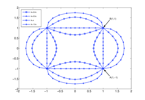
Figure 3: Curves ${\mathfrak{L}}_{4}(\theta)$ for various $\theta$.

Now our numerical experiments can be described as follows. First, we divide the interval $[0.1\pi,1.9\pi]$ by the points $\{\theta_{k}\}$, where $\theta_{k}=\pi(0.1+k\times 0.01)$. For every family of the test contours ${\mathfrak{L}}_{j}(\theta_{k}),\theta_{k}\in[0.1\pi,1.9\pi]$, $j=1,2,4$ consider the spline Galerkin methods with $n=256$ based on the splines of order $0,1$ or $2$. Compute then the condition numbers of the corresponding linear algebraic systems described by (5). Should there appear any point $\theta^{*}$ in the vicinity of which the condition numbers become large, a neighborhood of $\theta^{*}$ is refined by a smaller step $0.001\pi$, and condition numbers are recalculated with $n$ changed to $512$. The outcome of our computations is presented in Figure 4. In all cases, one can observe the absence of peaks in the graphs, which means that the Galerkin methods under consideration do not have ”critical” angles in the interval $[0.1\pi,1.9\pi]$. In other words, if the opening angles of all corners of the integration contour are located in the interval $[0.1\pi,1.9\pi]$, the spline Galerkin methods based on the splines of degree $0,1$ or $2$ are always stable. Another remarkable feature is that for the Galerkin methods based on the splines of the same degree, all graphs are of the same shape and for any $\theta\in[0.1\pi,1.9\pi]$ the corresponding condition numbers are very close. This suggests a conjecture that the condition numbers of the Galerkin methods possess certain ”locality” properties. They rather depend on the value of the critical angles present than on the shape of the curves used.

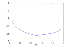
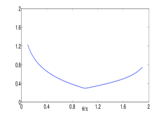
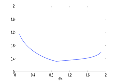
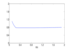
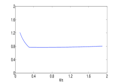
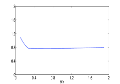
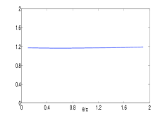
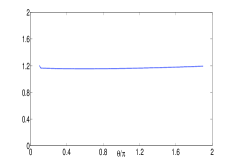
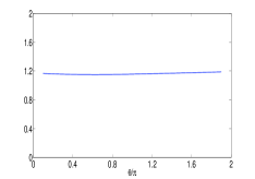
Figure 4: Logarithm $\log_{10}$ of condition numbers versus opening angles for Galerkin methods with $n=256$ for various contours and spline spaces. Left: contour ${\mathfrak{L}}_{1}$; Middle: contour ${\mathfrak{L}}_{2}$; Right: contour ${\mathfrak{L}}_{4}$; First row: $d=0$; Second row: $d=1$; Third row: $d=2$

Note that all numerical experiments are performed in MATLAB environment(version 7.9.0) and executed on an Acer Veriton M680 workstation equipped with a Intel Core i7 vPro 870 processor and 8GB of RAM. These are time consuming computations and it took from one to two weeks of computer work to obtain data for each graph in Figure 4 .

5 Conclusion

In this work, necessary and sufficient conditions of the stability of the spline Galerkin method for double layer potential equations on simple piecewise smooth contours are established. The theoretical results are verified by using curves with different number of corner points and numerical results are in a good correlation with theoretical studies. It turns out that the spline Galerkin methods based on splines of degrees $0,1,2$ are always stable and the convergence rates of the methods are comparable with other works.

6 Acknowledgement

The authors would like to thank an anonymous referee for constructive criticism and helpful suggestions.

References

- [1] G. R. Allan, Ideals of vector-valued functions, Proc. London Math. Soc. 18 (3) (1968) 193–216.
- [2] K. E. Atkinson, The numerical solution of integral equations of the second kind, Vol. 4 of Cambridge Monographs on Applied and Computational Mathematics, Cambridge University Press, Cambridge, 1997. http://dx.doi.org/10.1017/CBO9780511626340
- [3] G. A. Chandler, Galerkin’s method for boundary integral equations on polygonal domains, J. Austral. Math. Soc. Ser. B 26 (1984), 1-13.
- [4] M. Costabel, Boundary integral operators on Lipschitz domains: elementary results, SIAM J. Math. Anal. 19 (3) (1988) 613–626. http://dx.doi.org/10.1137/0519043
- [5] M. Costabel, E. P. Stephan, Boundary integral equations for mixed boundary value problems in polygonial domains and Galerkin approximations, in Banach Center Publications, Vol. 15, PWN, Warsaw, 1985.
- [6] M. Costabel, E. P. Stephan, On the convergence of collocation methods for boundary integral equations on polygons, Math. Comp., 49 (1987), pp. 461 – 478.
- [7] C. De Boor, A practical guide to splines, Springer Verlag, New-York-Heidelberg-Berlin, 1978.
- [8] V. D. Didenko, B. Silbermann, Approximation of additive convolution-like operators. Real -algebra approach. Frontiers in Mathematics, Birkhäuser Verlag, Basel, 2008. http://dx.doi.org/10.1137/0732086
- [9] V. D. Didenko, J. Helsing, Stability of the Nyström method for the Sherman-Lauricella equation, SIAM J. Numer. Anal. 49 (3) (2011) 1127–1148. http://dx.doi.org/10.1137/100811829
- [10] V. D. Didenko, J. Helsing, Features of the Nyström method for the Sherman-Lauricella equation on piecewise smooth contours, East Asian J. Appl. Math. 1 (4) (2011) 403–414.
- [11] V. D. Didenko, J. Helsing, On the stability of the Nyström method for the Muskhelishvili equation on contours with corners, SIAM J. Numer. Anal. 51 (3) (2013) 1757–1776. http://dx.doi.org/10.1137/120889472
- [12] V. D. Didenko, T. Tang, A. M. Vu, Spline Galerkin methods for the Sherman-Lauricella equation on contours with corners, SIAM J. Numer. Anal. 53 (6) (2015) 2752–2770. http://dx.doi.org/10.1137/140997968
- [13] V. D. Didenko, A. M. Vu, The Nyström method for the double layer potential equation on contours with corners. ArXiV:1410.3044.
- [14] V. D. Didenko, E. Venturino, Approximation method for the Muskhelishvili equation on smooth curves, Math. Comp., 76(259) 1317–1339, 2007.
- [15] R. V. Duduchava, Integral equations in convolution with discontinuous presymbols, singular integral equations with fixed singularities, and their applications to some problems of mechanics. BSB B. G. Teubner Verlagsgesellschaft, Leipzig, 1979.
- [16] I. G. Graham, G. A. Chandler, High-order methods for linear functionals of solutions of second kind integral equations, SIAM J. Num. Anal., 25 (1988), pp. 1118-1179.
- [17] J. Helsing, A fast and stable solver for singular integral equations on piecewise smooth curves, SIAM J. Sci. Comp., 33 (2011), 153–174.
- [18] J. Helsing, R. Ojala, Corner singularities for elliptic problems: Integral equations, graded meshes, quadrature, and compressed inverse preconditioning, J. Comput. Phys., 227 (2008), 8820–8840.
- [19] R. Kress, I. Sloan, F. Stenger, A sinc quadrature method for the double-layer integral equation in planar domains with corners, J. Integral Equations Appl., 10(3), 1998.
- [20] R. Kress, Linear integral equations, 3rd Edition, Vol. 82 of Applied Mathematical Sciences, Springer, New York, 2014. http://dx.doi.org/10.1007/978-1-4614-9593-2
- [21] R. Kress, A Nyström method for boundary integral equations in domains with corners, Numer. Math. 58 (1990), pp. 145-161.
- [22] Y. Jiang, B. Wang and Y. Xu, A fast Fourier-Galerkin method solving a boundary integral equation for the biharmonic equation, SIAM J. Numer. Anal., 52 (2014), 2530–2554.
- [23] N. I. Muskhelishvili, Singular integral equations, Nauka, Moscow, 1968.
- [24] S. Prössdorf, B. Silbermann, Numerical analysis for integral and related operator equations, Birkhäuser Verlag, Berlin–Basel, 1991.
- [25] S. Roch, P. A. Santos, B. Silbermann, Non-commutative Gelfand theories. A tool-kit for operator theorists and numerical analysts. Universitext, Springer-Verlag London Ltd., London, 2011.
- [26] I. B. Simonenko, and C. N. Min’, A local method in the theory of one-dimensional singular integral equations with piecewise continuous coefficients. Noethericity. Rostov. Gos. Univ., Rostov, 1986, (in Russian).
- [27] G. Verchota, Layer potentials and regularity for the Dirichlet problem for Laplace’s equation in Lipschitz domains, J. Funct. Anal. 59 (3) (1984) 572–611. http://dx.doi.org/10.1016/0022-1236(84)90066-1