Diagnosing shock temperature with NH₃ and H₂O profiles

Abstract

In a previous study of the L1157 B1 shocked cavity, a comparison between NH₃(1₀-$0_{0}$) and H₂O(1₁₀–1₀₁) transitions showed a striking difference in the profiles, with H₂O emitting at definitely higher velocities. This behaviour was explained as a result of the high-temperature gas-phase chemistry occurring in the postshock gas in the B1 cavity of this outflow. If the differences in behaviour between ammonia and water are indeed a consequence of the high gas temperatures reached during the passage of a shock, then one should find such differences to be ubiquitous among chemically rich outflows. In order to determine whether the difference in profiles observed between NH₃ and H₂O is unique to L1157 or a common characteristic of chemically rich outflows, we have performed Herschel-HIFI observations of the NH₃(1₀-0₀) line at 572.5 GHz in a sample of 8 bright low-mass outflow spots already observed in the H₂O(1₁₀–1₀₁) line within the WISH KP. We detected the ammonia emission at high-velocities at most of the outflows positions. In all cases, the water emission reaches higher velocities than NH₃, proving that this behaviour is not exclusive of the L1157-B1 position. Comparisons with a gas-grain chemical and shock model confirms, for this larger sample, that the behaviour of ammonia is determined principally by the temperature of the gas.

Table 1: Source list and observed positions.

Source	$\alpha_{\rm J2000}$	$\delta_{\rm J2000}$	$V_{\rm LSR}$	$L_{\rm bol}$	$d$	Offsets Blue/Red
	(h m s)	(o $\arcmin$ $\arcsec$)	(km s-1)	($L_{\odot}$)	(pc)	(arcsec)
L1448	03 25 38.9	+30 44 05	+4.7	6	235	B2(-13,+29), R4(+26,-125)
NGC1333-IRAS2A	03 28 55.4	+31 14 35	+6.0	25	235	B(-100,+25), R(+70,-15)
NGC1333-IRAS4A	03 29 10.4	+31 13 31	+6.5	8	235	B(-6,-19), R(+14,+25)
L1157	20 39 06.2	+68 02 16	+2.6	4	250	B2(+35,-95), R(-30,+125)

Note– For references to the coordinates and protostellar properties see Tafalla et al. 2013; for the distance estimation see Looney, Tobin & Kwon (2007) and Hirota et al. (2008).

1 Introduction

A newborn protostar generates a fast and well collimated jet, possibly surrounded by a wider angle wind. In turn, the ejected material drives (bow-)shocks travelling through the surrounding high-density medium and traced by H₂ ro-vibrational lines at excitation temperatures of around 2000 K. Consequently, slower and cold (10–20 K) molecular outflows are formed by swept-up material, usually traced by CO. Shocks heat the gas and trigger several processes such as endothermic chemical reactions and ice grain mantle sublimation or sputtering. Several molecules, such as H₂O, NH₃, CH₃OH, H₂CO, undergo spectacular enhancements by orders of magnitude in their abundances (van Dishoeck & Blake, 1998), as observed at mm-wavelengths in a number of outflows (Garay et al., 1998; Bachiller & Perez Gutierrez, 1997; Jørgensen et al., 2007). The link between the gas components at $\sim$ 10 K and the hot 2000 K shocked component is crucial to understand how the protostellar wind transfers momentum and energy back to the ambient medium. In this context, studies of the chemical composition of typical molecules in bow-shocks are essential because they represent a very powerful diagnostic tool for probing their physical conditions. Such studies are also paramount to get a comprehensive understanding of chemistry throughout the various phases of the interstellar medium.

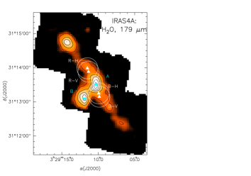
Figure 1: NGC 1333 IRAS4A outflow and corresponding observed positions. The background image represent the H₂O emission at 179 $\mu$m from the WISH program (Santangelo et al., 2014). The circles show the vertical (V) and horizontal (H) polarization HPBW at the observed positions, whose centers are indicated by the triangles. The stars mark the position of the continuum sources (A and B: Looney, Mundy & Welch, 2000).

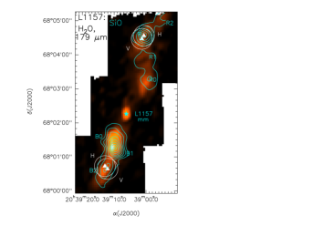
Figure 2: L1157 outflow and corresponding observed positions. The background image represent the H₂O emission at 179 $\mu$m from the WISH program (Nisini et al., 2010). The blue contours show the SiO emission from Bachiller et al. (2001). The circles show the vertical (V) and horizontal (H) polarization HPBW at the observed positions, whose centers are indicated by the triangles. The star marks the position of the central source (L1157-mm).

As part of the Herschel Key Program CHESS (Chemical Herschel Surveys of Star forming regions: Ceccarelli et al., 2010), the bow-shock L1157-B1 has been investigated with a spectral survey using the HIFI instrument. From the comparison between NH₃(1₀–0₀) and H₂O(1₁₀–1₀₁) profiles, a straightforward estimate of the relative abundance ratios of the gas at different velocities was obtained (Codella et al., 2010). As a notable example, the NH₃/H₂O intensity ratio decreases by a factor of $\sim$ 5 moving towards higher velocities suggesting, in case of optically thin emission along the wings, a similar decrease in the abundance ratios. Other tracers of shocked material such as CH₃OH and H₂CO show the same profile as that of NH₃. In Codella et al. (2010) we propose that the difference between the H₂O and other species reflects different formation mechanisms: for example, while the bulk of NH₃ is released from the grain mantles, H₂O is enhanced by the release of the icy mantles as well as by endothermic reactions occurring in the warm ($\geq 220$ K) shocked gas, which convert all gaseous atomic oxygen into water (e.g., Jiménez-Serra et al., 2008, and references therein). However, a model by Viti et al. (2011) made especially for these data set suggests that the differences observed in the profile of the different molecular tracers are due mainly to the temperature of the gas: if the latter undergoes a period at a temperature close to 4000 K, then NH₃ is easily destroyed by the reaction with hydrogen which leads to NH₂ $+$ H₂ (this reaction has a high barrier of $\sim$5000 K), while H₂O remains high in abundance. Such scenario can be explained by the presence of a C-type shock whose pre-shock density and velocity are such that the maximum temperature of the shock reaches 4000 K along the B1 shock of L1157. These findings called for observations of more molecular shocked regions associated with protostellar outflows to investigate whether the difference in profiles between H₂O and other species are unique to L1157 or whether it is an ubiquitous characteristic of chemically rich outflows.

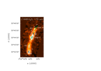
Figure 3: L1448 outflow and corresponding observed positions. The background image represent the H₂O emission at 179 $\mu$m from the WISH program (Nisini et al., 2013). The circles show the vertical (V) and horizontal (H) polarization HPBW at the observed positions, whose centers are indicated by the triangles. The green crosses indicate the positions of the millimeter continuum sources (N, S, A, B, and W: Kwon et al., 2006).

In this article we present observations of the $J_{K}=$1₀–0₀ transition of ortho-NH₃ at 572.5 GHz in a number of outflow spots already observed in the ortho-H₂O(1₁₀–1₀₁) line as part of the Herschel Key Program WISH (Water In Star-forming regions with Herschel: van Dishoeck et al., 2011) and reported by Tafalla et al. (2013). In Sect. 2 the target selection and Herschel observations with HIFI are described, in Sect. 3 we report the line profiles obtained, in Sect. 4 and 5 we develop the analysis of the data, and in Sect. 6 we present the summary and conclusions.

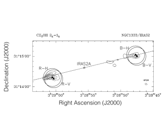
Figure 4: NGC1333 IRAS2A outflow and corresponding observed positions (image adapted from Bachiller et al., 1998). The contours show the CH₃OH ($2_{k}-1_{k}$) PdBI map. The circles show the vertical (V) and horizontal (H) polarization HPBW at the observed positions, whose centers are indicated by the triangles. The star indicates the position of the central source (IRAS2A).

2 Observations

2.1 Targeted outflow positions

The WISH protostellar outflow sample contains 26 outflows driven by Class 0/I low-mass Young Stellar Objects (Tafalla et al., 2013). For each source, two ’hot’ spots (blue- and red-shifted) have been observed. The positions were carefully selected by inspecting the maps obtained from ground-based facilities using typical tracers of shocked material (e.g. high-velocity CO, CH₃OH, SiO, H₂CO). The selected spots are associated with a definite enhancement of the abundance of molecules tracing shocked material or with high-velocity molecular components (up to about 100 km s^-1 with respect to the systemic velocity).

From the WISH survey we selected a sample containing 8 ’hot’ spots in shocks associated with four ’classical’ flows driven by low-mass Young Stellar Objects (YSOs) in the earliest evolutionary stages (Class 0), and associated with bright H₂O emission: L1448, L1157, NGC1333-IRAS2A, NGC1333-IRAS4A (see Table 1). These YSOs are approximately at the same distance from Earth, with bolometric luminosities between 4-25 $L_{\rm bol}$.

2.2 HIFI Observations

The observations were carried out with the band 1b of the HIFI instrument on-board Herschel, during 2011 October and December, and 2012 February, as part of an OT-1 observing program (OT1_ccodella_1). The observations log is shown in Table 2. The pointed positions are shown in Table 1 and indicated on Figs. 1–4. The single-pointing observations were made in Position Switching mode and with spatial offsets derived by inspecting large-scale CO maps in order to avoid off-source contamination.

Table 2: HIFI band 1b observations.

Target	Duration	Date	Obs. Id
	(seconds)
L1448-R4	5703	2012-02-24	1342239631
L1448-B2	5703	2012-02-24	1342239632
IRAS4A-B	5703	2012-02-25	1342239633
IRAS4A-R	5703	2012-02-25	1342239634
IRAS2A-B	5703	2012-02-25	1342239635
IRAS2A-R	5703	2012-02-25	1342239636
L1157-R	12828	2011-12-22	1342235065
L1157-B2	5703	2011-10-08	1342230366

The Wide Band Spectrometer (WBS) was used with a frequency resolution of 1.1 MHz. Two High Resolution Spectrometers (HRS) were used in parallel with a frequency resolution of 250 kHz. The observing set-up was prepared in order to observe the o–NH₃(1₀–0₀) line in lower side band with both the WBS as well as with one HRS unit. In addition to our target line, we observed the CS(12–11) line at 587.6 GHz in the upper side band with the WBS and the second HSR unit, and the CO(5–4) line at 576.3 GHz in lower side band with the WBS. Also, the a–CH₃OH (12_1,11–11_1,10) line at 584.8 GHz and the p–H₂CO (8_2,6–7_2,5) at 587.4 GHz were observed in the upper side band with the WBS only. Both H and V polarization were observed and then averaged to increase sensitivity. However, we caution that H and V pointings were separated by 6$\aas@@fstack{\prime\prime}$6 and therefore each polarization may cover a slightly different region. Thus our analysis refers to the whole area covered by the two beams. In appendix A we provide and discuss the H and V spectra. The molecular line parameters as well as Herschel’s antenna HPBW, taken according to Roelfsema et al. (2012), are reported in Table 3. The Herschel observations were processed with the ESA-supported package HIPE 8.10 (Herschel Interactive Processing Environment; Ott, 2010). FITS files from level 2 were then created and transformed into GILDAS format for data analysis.

The spectra in this article are reported in units of main-beam brightness temperature (T${}_{\rm MB}=$T${}_{A}^{*}\times$ $F_{\rm eff}$/$B_{\rm eff}$), for which we have used the $F_{\rm eff}$ of 0.96 and $B_{\rm eff}$ of 0.76 (nominal for band 1b) for all the lines, according to Roelfsema et al. (2012). After smoothing, the spectral resolution in all the cases is 0.5 km s^-1.

Table 3: Transitions and parameters of the lines observed.

Transitiona	$\nu_{\rm 0}$	$E_{\rm u}$	$A_{\rm ij}$	HPBW
	(GHz)	(K)	(10-3s-1)	(′′)
o–NH3(10–00)	572.498	28	1.61	37
CO(5–4)	576.267	83	0.01	37
CH3OH(121,11–111,10)A+	584.822	197	0.89	36
p–H2CO(82,6–72,5)	587.453	173	5.66	36
CS(12–11)	587.616	183	4.34	36
o–H2O(110–101)b	556.936	61	3.46	39

^a Transition properties are taken from the Cologne Database for Molecular Spectroscopy: Müller et al. (2005). ^b Taken from Tafalla et al. (2013)

3 Results

Table 4: Line properties.

Transitiona	$T_{\rm MB}^{\rm peak}$	r.m.s.	$V_{peak}$	$V_{min},V_{max}$b	$\int$ $T_{\rm MB}dv$c
	(mK)	(mK)	(km s-1)	(km s-1)	(mK km s-1)
IRAS4A-B
o–NH3(10–00)	280(4)	4	+5.7(0.5)	$-$9.0, $+$12.7	624(10)
o–H2O(110–101)	852(2)	2	+1.1(0.5)	$-$15.9, $+$25.1	14237(9)
CO(5–4)	5131(2)	2	+6.0(0.5)	$-$18.1, $+$49.7	29472(12)
CH3OH(121,11–111,10) A+	30(3)	3	+6.2(0.5)	$+$0.9, $+$9.6	130(7)
p–H2CO(82,6–72,5)	20(3)	3	+5.7(0.5)	$+$3.0, $+$7.8	88(7)
CS(12–11)	46(3)	3	+3.3(0.5)	$-$5.6, $+$13.3	532(9)
IRAS4A-R
o–NH3(10–00)	220(4)	4	+5.5(0.5)	$-$4.8, $+$24.2	721(8)
o–H2O(110–101)	532(2)	2	+10.5(0.5)	$-$1.7, $+$31.9	7263(8)
CO(5–4)	4604(2)	2	+6.0(0.5)	$-$12.3, $+$51.5	28245(12)
CH3OH(121,11–111,10) A+	30(4)	4	+8.0(0.5)	$+$4.9, $+$12.0	130(8)
p–H2CO(82,6–72,5)	30(3)	3	+7.8(0.5)	$+$6.1, $+$10.1	77(9)
CS(12–11)	51(3)	3	+8.2(0.5)	$+$5.0, $+$19.4	379(10)
IRAS2A-B
o–NH3(10–00)	50(4)	4	+8.5(0.5)	$-$5.0, $+$9.0	413(11)
o–H2O(110–101)	565(2)	2	+0.2(0.5)	$-$11.2, $+$7.6	6427(6)
CO(5–4)	1063(3)	2	+5.5(0.5)	$-$16.1, $+$6.2	6427(7)
CH3OH(121,11–111,10) A+	–	3	–	–	–
p–H2CO(82,6–72,5)	–	3	–	–	–
CS(12–11)	–	2	–	–	–
IRAS2A-R
o–NH3(10–00)	190(4)	4	+6.5(0.5)	$+$4.5, $+$19.2	858(14)
o–H2O(110–101)	581(2)	2	+11.5(0.5)	$+$3.2, $+$28.5	7182(8)
CO(5–4)	5832(3)	3	+6.7(0.5)	$-$11.8, $+$33.3	33186(9)
CH3OH(121,11–111,10) A+	20(3)	3	+10.0(0.5)	$+$8.3, $+$10.7	64(7)
p–H2CO(82,6–72,5)	–	4	–	–	–
CS(12–11)	9(3)	3	+10.0(0.5)	$+$7.2, $+$11.4	44(4)
L1448-B2
o–NH3(10–00)	120(4)	4	+4.2(0.5)	$+$2.7, $+$6.3	295(8)
o–H2O(110–101)	348(2)	2	$-$1.1(0.5)	$-$61.7, $+$5.5	8911(11)
CO(5–4)	2711(3)	3	+3.5(0.5)	$-$77.3, $+$35.8	31603(9)
CH3OH(121,11–111,10) A+	–	3	–	–	–
p–H2CO(82,6–72,5)	–	4	–	–	–
CS(12–11)	–	3	–	–	–
L1448-R4
o–NH3(10–00)	20(3)	4	+10.2(0.5)	$+$6.3, $+$18.8	179(14)
o–H2O(110–101)	406(1)	1	+19.5(0.5)	$+$1.3, $+$47.4	11388(6)
CO(5–4)	1936(03)	3	+6.2(0.5)	$-$1.1, $+$51.5	18381(10)
CH3OH(121,11–111,10) A+	–	4	–	–	–
p–H2CO(82,6–72,5)	–	4	–	–	–
CS(12–11)	–	4	–	–	–
L1157-B2
o–NH3(10–00)	130(4)	4	+1.1(0.5)	$-$4.5, $+$5.5	717(9)
o–H2O(110–101)	1150(5)	5	+4.5(0.5)	$-$6.6, $+$9.4	9274(13)
CO(5–4)	6394(2)	2	+1.9(0.5)	$-$15.2, $+$9.1	21733(7)
CH3OH(121,11–111,10) A+	–	4	–	–	–
p–H2CO(82,6–72,5)	–	3	–	–	–
CS(12–11)	–	4	–	–	–
L1157-R
o–NH3(10–00)	40(4)	4	+7.6(0.5)	$+$2.2, $+$18.7	383(13)
o–H2O(110–101)	360(5)	5	+19.3(0.5)	$-$1.1, $+$30.5	6651(20)
CO(5–4)	2323(2)	2	+4.1(0.5)	$-$2.9, $+$33.5	21975(8)
CH3OH(121,11–111,10) A+	–	3	–	–	–
p–H2CO(82,6–72,5)	–	2	–	–	–
CS(12–11)	–	4	–	–	–

^a Apart from the transitions reported in Table 3, included here is the o–H₂O transition taken from Tafalla et al. (2013). ^b Velocity boundaries where the emission is $\geq$ 3$\sigma$. ^c The integrated area between $V_{min}$ and $V_{max}$.

Table 4 summarizes the results of the observations, indicating the line intensities ($T_{\rm MB}^{\rm peak}$), velocity of the peak ($V_{\rm peak}$), velocity limits of the emission ($V_{min},V_{max}$), and the total integrated emission ($\int$ $T_{\rm MB}dv$). Table 4 also reports the same parameters for the H₂O line, which we measured from the spectra reported in Tafalla et al. (2013). We computed the column densities, from the total integrated emission, assuming LTE and optically thin emission. Table 6 shows the results assuming a typical range of temperatures observed toward these kind of objects (20-100 K, e.g., Lefloch et al., 2012; Tafalla et al., 2013). We find that the ammonia column densities are in the range of $\sim$ 10¹⁰–5$\times$10¹¹ cm^-2. To probe that these estimations are accurate, in Appendix B we present the results of radiative transfer calculations showing that the ammonia emission is optically thin, $\tau$ $\leq$ 1.3 $\times$ 10^-2, for these values of column densities and temperatures (see Fig. 14). For CS, CO, CH₃OH, and H₂CO, the column densities ranges are $\sim$ 10¹²–5$\times$10¹⁴ cm^-2, 10¹⁵–7$\times$10¹⁶, 8$\times$10¹²–8$\times$10¹⁵, and 9$\times$10¹¹–9$\times$10¹³ cm^-2, respectively. Note that in the case of CO, due to the strong absorption, the numbers are only lower limits.

3.1 NH₃ Profiles

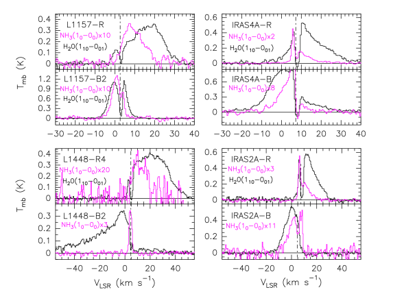
Figure 5: The WBS NH₃ spectra (magenta) at the different observed positions. Also displayed are the ortho–H₂O spectra (black) from Tafalla et al. (2013). Dashed vertical lines indicates the cloud velocity.

The ammonia WBS spectra observed at each of the outflow positions are shown in Fig. 5, overlaid on the corresponding water spectra. Ammonia emission was detected in all positions, showing extended line wings (up to $\sim$ 15 km s^-1 with respect to the systemic velocity) in all but the L1448-B2 position, where we found just a narrow profile (a peculiar feature discussed in Sect. 4). With the exception of L1448-B2, the WBS spectra show an absorbing dip at systemic velocity plausibly due to the absorption from the extended envelope of the protostar.

The high resolution spectra, from the HRS, do not show additional information on the low-velocity NH₃ emission already provided by the WBS spectra, with the exception of L1448-B2, which shows multiple peaks at low velocities (Fig. 6). The Horizontal and Vertical polarization spectra are slightly different, as the result of the different area covered by each of them (see Sect. 2.2). The two most prominent spectral features are seen in the Vertical polarization spectrum (which correspond to the beam closer to the central region), showing peaks at 4.0 and 4.7 km s^-1. These spectral features are discussed in Sect. 4 and 5.

3.2 CS, H₂CO, and CH₃OH profiles

The spectra of all observed lines are presented in Figs. A1–A4. Only in IRAS4A-B and IRAS4A-R the CS, H₂CO, and CH₃OH transitions were found. These two positions are also the strongest line emitters among the sources studied here. This is possibly due to the chemical richness of this source as reported by previous investigations (e.g., Wakelam et al., 2005; Santangelo et al., 2014). However, we point out that later might also be due to sensitivity. We notice that these transitions have larger column densities than NH₃. In general, we see that the CS, H₂CO, and CH₃OH transitions have profiles more similar to NH₃ than to H₂O, in particular in terms of the maximum velocity. While a more detailed analysis of such species is out of the scope of the present paper, we shall briefly discuss these species in Section 5.

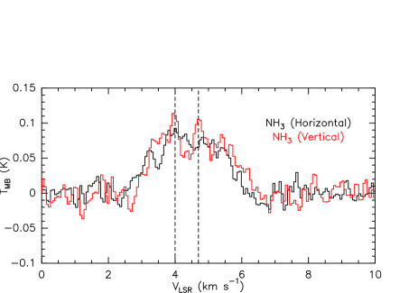
Figure 6: High spectral resolution (HRS) NH₃ spectrum towards L1448-B2. Horizontal and Vertical polarization are shown in black and red, respectively. The vertical dashed lines indicate the velocities of the two clouds (4.0 km s^-1 and 4.7 km s^-1) found in ammonia centimeter transitions by Bachiller & Cernicharo (1986).

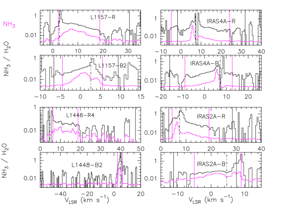
Figure 7: The NH₃/H₂O intensity ratio at the different observed positions. Dashed vertical lines indicate the cloud velocity. To indicate the region where the ratio is valid, the velocity boundaries (V_min,V_max) where the NH₃ and H₂O emission is $\geq$ 3$\sigma$ are indicated by vertical lines, in magenta and black, respectively. The NH₃ spectra are shown in magenta as a reference.

4 Ammonia versus water

In order to properly compare the ammonia and water profiles, a more complete radiative transfer analysis of both species would be necessary to discard excitation and opacity effects. Such analysis is out of the scope of the present work, since we only have one NH₃ transition. Despite that, we have shown in Appendix B that our NH₃ transition is optically thin at the positions here investigated, and Tafalla et al. (2013), based on the analysis of two H₂O transitions, provided evidence that the water emission is also optically thin at the same positions. In addition, radiative transfer models from Tafalla et al. (2013) revealed a water gas component with a density in the range of 10⁷–10⁸ cm^-3, and therefore close to critical density of our NH₃ transition ($\sim$10⁸ cm^-3, e.g. Menten et al., 2010). All these information give confidence that the line profile comparison presented in the following is appropriate. We also caution in sect. 5 on the need of radiative transfer calculations in the context of the chemical models.

From the comparison between the NH₃ and H₂O spectra we see that the profiles of the two species are more often different in shape and in maximum velocity. In all positions the maximum terminal velocity ($V_{\rm ter}$) reached by NH₃ is lower than in H₂O (always by more than a factor of two; see Fig. 8), which then confirm this tendency first found in L1157-B1 by Codella et al. (2010). The more prominent cases are L1157-R and L1448-B2, which show either a considerably different $V_{\rm peak}$ or very different linewidths.

The ammonia-to-water line ratio, as function of velocity, is shown in Fig. 7. The maximum line ratio is found around the cloud velocity in all but IRAS2A-B position. In the L1157-B2 and L1157-R positions the behaviour of the line ratio as a function of velocity is similar to what was found by Codella et al. (2010) at the L1157-B1 position, i.e. a maximum close to the cloud velocity and slow decrease of the ratio toward high velocities.

The most peculiar case is the L1448-B2 position, in which the line ratio profile is just a sharp peak at the systemic velocity. This is the consequence of the very different NH₃ line profile with respect to H₂O, as pointed out previously. Here the main difference is that while the H₂O reaches V${}_{\rm LSR}\sim-$ 61 km s^-1, the NH₃ reaches only V${}_{\rm LSR}\sim+$3 km s^-1 (with linewidths of $\sim$ 67 and 4 km s^-1, respectively). As pointed out in the previous section, the high spectral resolution data (Fig. 6) reveal structure of this narrow profile: at least two peaks, at 4.0 and 4.7 km s^-1.

Similar narrow profiles were also found by Jiménez-Serra et al. (2005) in CH₃OH millimeter transitions at other nearby positions in the blue lobe of L1448, which they interpret as the magnetic precursor (see also Jiménez-Serra et al., 2004, 2009). However, the spectral feature of such precursor is very narrow ($\sim$ 0.6 km s^-1) and red-shifted by about 0.5 km s^-1 with respect to the 4.7 km s^-1 cloud, i.e. at V${}_{\rm LSR}\sim+$5.2 km s^-1. On the other hand, our NH₃ spectra is not that narrow (in fact, a few km s^-1) and does not show a peak at that V_LSR. We notice that our peaks are coincident with the peak velocities of the clouds previously reported in centimeter ammonia transitions by Bachiller & Cernicharo (1986). Taking into account the discrepancy between the H and V polarization (the two peaks only clearly noticed in the V polarization) and the noise, it does not seem reliable to identify the narrow feature as the magnetic precursor. Although the noisy high resolution spectra might not be sufficient evidence, our ammonia observations of the L1448-B2 position suggest that the emission may be tracing these two clouds enclosed within the HIFI beam. An additional argument for the absence of ammonia emission from the high-velocity shock is that in previous NH₃(1,1) and (2,1) interferometric maps by Curiel et al. (1999), no emission from the B2 position was found, with the maps showing emission only towards the central part of L1448-C and L1448-N objects. This peculiar narrow line profile is further discussed, in its comparison with the water profile, within the context of the chemical models in Sect. 5.

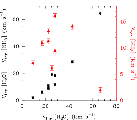
Figure 8: Comparison between the maximum (terminal, $V_{\rm ter}$) velocity (absolute values with respect to the systemic velocity, see Table 4) of the H₂O emission at 179 $\mu$m and that of NH₃ at 572 GHz. Black points show the comparison between $V_{\rm ter}$[H₂O]–$V_{\rm ter}$[NH₃] versus $V_{\rm ter}$[H₂O], while red points compares $V_{\rm ter}$[NH₃] with $V_{\rm ter}$[H₂O].

5 Chemical models

The NH₃-H₂O profile differences first discovered in L1157-B1 (e.g. Codella et al. 2010) are clearly present in other outflows. In Viti et al. (2011) a gas-grain chemical and shock model was used to investigate the differences in profile between the water and the ammonia transitions; it was found that these differences are purely chemical and can be explained by the presence of a C-type shock whose maximum temperature must be close to $\sim$4000 K along the B1 clump. More specifically, assuming, as Codella et al. (2010) imply, that the NH₃/H₂O intensity ratio decreases at high velocities because a similar decrease in the abundance ratios occurs, then models where the maximum temperature of the shock is close to $\sim$4000K lead to water remaining abundant at all velocities (i.e. throughout the C-shock) while NH₃ decreases at high velocities in the warm postshock gas. This is due to i) the efficient destruction of ammonia in the postshock gas via the endothermic reaction H $+$ NH₃ $\rightarrow$ NH₂ $+$ H₂ once its activation barrier ($\sim$5000 K) is overcome at temperatures higher than $\sim$4000 K (see Viti et al. 2011); and ii) to the absence of formation routes of NH₃ at high temperature. In Viti et al. (2011) the models that best fit the NH₃/H₂O also fit the emission from other shock tracers such as CH₃OH and H₂CO, which fairly follow the behaviour of ammonia (see also Section 3.2 for the case of these molecules in this work). Due to the few detections of the later molecules and the low signal-to-noise in their wings, we do not further discuss them here in the context of the models.

The maximum temperature of the shock in turn constrains the pre-shock density of the clump and velocity of the shock. If the temperature of the gas is indeed the key physical parameter determining the amount of ammonia as a function of velocity, then, outflows spots differing in pre-shock density and shock velocities will have different profile behaviours for NH₃ and hence different water-to-ammonia ratios as a function of velocities.

To illustrate this, in Figure 8 we report the difference between the terminal velocities of H₂O and NH₃ as a function of the terminal velocity of H₂O. Since the abundance of H₂O remains high across the full shock width (Viti et al. 2011), we use the terminal velocity of the H₂O line profile as a proxy of the velocity of the C-shock. We note that this is strictly true for shock velocities between 10 and 45 km s^-1, i.e. for the majority of the shock spots discussed in this paper (see Section 5.2 below). Therefore, we assume that the terminal velocity of H₂O lies closely to the actual velocity of the shock. As a result, from Figure 8 we find that the terminal velocities of water and ammonia become more unlike for increasing C-shock velocities, suggesting a clear chemical effect for ammonia with the strength of the shock. In this section we test this hypothesis by using the Viti et al. (2011) model and by determining a set of physical and shock parameters that can fit each of the spectra.

5.1 The shock and chemical model

The code used in Viti et al. (2011) is the UCL$\_$CHEM (Viti et al., 2004) augmented with a shock module (from Jimenez-Serra et al. 2008). The code runs essentially in two phases: Phase I follows the evolution of a core, with initial density of 100 cm^-3, gravitationally collapsing; gas-phase chemistry, sticking on to dust particles with subsequent surface processing occur. The sticking coefficients for all species are all assumed to be 1, equivalent to a 100% sticking efficiency (see Rawlings et al., 1992, Equation 2). However for consistency with the Viti et al. (2011) study, we have varied these coefficients in order to simulate different degree of freeze out at the end of Phase I. The final density is a free parameter (see below). Note that the collapse in Phase I is not meant to represent the formation of a protostar, but it is simply a way to compute the chemistry of high density gas in a self-consistent way starting from a diffuse atomic gas, i.e. without assuming the chemical composition at its final density. Phase II computes the time-dependent chemical evolution of the gas and dust once the core has formed and stellar activity and shocks are present. The model self-consistently accounts for both thermal desorption, due to the dust being heated by the presence of the outflow, as well as sputtering of the icy mantles: the latter are sputtered once the dynamical age across the C-shock has reached the ”saturation timescales” ($t_{sat}$; see Table 5), as in Jimenez-Serra et al. (2008). In all the cases considered, sputtering occurs at earlier times than thermal desorption. The model is the same as employed in Viti et al. (2011) to model the same shock spot so we refer the reader to that paper for further details.

For this work, we ran a grid of models varying in (i) pre-shock density (n_H); (ii) shock velocity (v_shock); (iii) efficiency of freeze out of gas phase species during the cold phase (Phase I). The maximum temperature of the shock, which varies depending on the pre-shock density and shock velocity, is extracted from Figures 8b and 9b in Draine, Roberge & Dalgarno (1983). The saturation times are taken from Jimenez-Serra et al. (2008). Table 5 lists the models ran. Columns 7 lists, for each model, the length of the dissipation region which is the shock length scale and depends on the shock velocity as well as on the pre-shock density.

Table 5: Model parameters: Model number, pre-shock density, shock velocity, saturation time, maximum temperature of the neutral gas (these four parameters are interconnected - see Jimenez-Serra et al. 2008), degree of depletion (note that we use the fraction of CO in the icy mantles at the end of Phase I to estimate this fraction), and dissipation length. The last column lists the group we categorized the model in (see Sect. 5.1). a(b) stands for a $\times$ 10^b.

no	nH (cm-3)	Vs (km s-1)	tsat (yrs)	Tmax (K)	Freeze-out (%)	Ldiss (cm)	Group
1	105	40	4.6	4000	1	1.5(16)	2
2	105	40	4.6	4000	15	1.5(16)	2
3	105	40	4.6	4000	30	1.5(16)	2
4	105	35	4.6	3200	30	1.3(16)	1
5	105	35	4.6	3200	1	1.3(16)	1
6	103	40	455	2200	1	1.5(18)	1
7	104	40	45.5	2200	1	1.5(17)	1
8	104	60	38	4000	3	2.2(17)	2
9	103	60	380	4000	3	2.2(18)	2
10	103	60	380	4000	1	2.2(18)	2
11	105	40	4.6	4000	60	1.5(16)	2
12	104	40	45.5	2200	6	1.5(17)	1
13	105	35	4.6	3200	60	1.3(16)	1
14	104	10	10.5	300	18	3.7(16)	1
15	104	40	45.5	2200	18	1.5(17)	1
16	103	10	954	300	1	3.7(17)	3
17	104	10	10.5	300	3	3.7(16)	1
18	105	10	10.5	300	60	3.7(15)	1
19	105	10	10.5	300	30	3.7(15)	1
20	105	10	10.5	300	15	3.7(15)	1
21	105	10	10.5	300	1	3.7(15)	1
22	103	20	570	900	1	7.4(17)	3
23	103	20	570	900	3	7.4(17)	3
24	104	20	5.7	900	3	7.4(16)	3
25	104	20	5.7	900	18	7.4(16)	1
26	104	20	57.0	900	18	7.4(16)	1
27	104	20	57.0	900	3	7.4(16)	1
28	105	20	5.7	800	15	7.4(15)	1
29	105	20	5.7	800	1	7.4(15)	1
30	105	20	5.7	800	60	7.4(15)	1
31	105	20	5.7	800	30	7.4(15)	1
32	104	10	95.4	300	18	3.7(16)	1
33	104	10	95.4	300	3	3.7(16)	1
34	106	40	0.5	4000	100	1.5(15)	1
35	106	40	0.5	4000	50	1.5(15)	2
36	106	40	0.5	4000	80	1.5(15)	2
37	103	30	440	1800	1	1.1(18)	2
38	106	30	0.4	2000	80	1.1(15)	3
39	103	30	440	1800	3	1.1(18)	3
40	104	30	44.0	1800	18	1.1(17)	1
41	104	30	44.0	1800	3	1.1(17)	1
42	106	30	0.4	2000	100	1.1(18)	1
43	106	30	0.4	2000	50	1.1(18)	1
44	105	30	4.4	2000	30	1.1(16)	1
45	105	30	4.4	2000	1	1.1(16)	1
46	105	30	4.4	2000	6	1.1(16)	1
47	105	30	4.4	2000	15	1.1(16)	1
48	104	15	68	600	18	5.5(16)	1
49	105	15	6.8	550	60	5.5(15)	1
50	106	15	0.7	550	80	5.5(14)	1
51	104	25	49	1200	18	9.2(16)	1
52	105	25	4.9	1500	60	9.2(15)	1
53	106	25	0.5	1500	80	9.2(14)	1
54	104	45	33.8	2800	18	1.7(17)	1
55	105	45	3.4	5000	60	1.7(16)	3
56	106	45	0.3	5000	80	1.7(15)	3
57	5$\times$104	45	6.7	6500	30	3.7(16)	3
58	104	65	38	10000	30	2.2(17)	3

5.2 Chemical trends

The behaviour of both water and ammonia for each model is analysed and we find that broadly speaking we can divide our models in three groups (see last column of Table 5):

• Group 1: models where ammonia and water behave in a similar way, i.e. they are both either abundant, or otherwise, at each position across the dissipation length; Models 4-7, 12-15, 17-21, 25-34, 40-54 belong to this category.

• Group 2: models where ammonia decreases ’earlier’ in the postshock gas (i.e at lower velocities) than water; Models 1-3, 8-11, 35-36 belong to this group.

• Group 3: models where the behaviour of NH₃ and/or water does not follow a clear trend. Models 16, 22-24, 37-39, 55-58 belong to this category.

In Figure 9 we plot the fractional abundance of water with respect to the total number of hydrogen nuclei (black line) and ammonia (red line) as a function of velocity within the postshock gas for a selected subset of models covering all the behaviours.

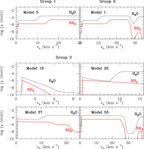
Figure 9: Fractional abundances with respect to the total number of hydrogen nuclei of water and ammonia as a function of velocity within the postshock gas, for representative models within each Group.

The behaviour of ammonia and water in Groups 1 and 2 were amply discussed in Viti et al. (2011). Group 3 includes models where the trend of water and ammonia are not easily categorized; for example in Model 16, both species decrease considerably but the water abundance does not drop as much as the ammonia one, and eventually reaches a plateau. Model 22, 23, 24 and 37 have the same behaviour of models belonging to Group 1 up to 7 km s^-1 but then water increases due to the temperature in the shock reaching above $\sim$200 K; ammonia on the other hand reaches a plateau: both species are in fact quite abundant throughout the dissipation length. Models 38 and 39 do show a decrease in ammonia as the velocity increases but without a sharp drop in its abundance, which remains constant at 10^-8. This decrease is again due to the high gas temperature reached in the shock, which allows the destruction of NH₃ to occur (Viti et al. 2011). The decrease of the NH₃/H₂O ratio for models 22, 23 and 24 is expected to be similar to that for models 38 and 39. However, the reactions responsible for this decrease are different: if the shock velocity is high, ammonia is destroyed (models 38 and 39), while if the shock velocity is low, water is enhanced (models 22, 23 and 24). In Models 55, 56, 57, 58, where the temperature of the gas is $\geq$ 5000 K, both water and ammonia decrease in abundance with velocity but then water increases again and remains high in abundance, while NH₃ only briefly increases in abundance: the higher the shock temperature, the larger and longer is the drop in water abundance.

The subdivision above is purely based on an empirical analysis of our plots. We now attempt at identifying the chemical or physical processes that yield such categorization. In Viti et al (2011) we claimed that the differences between NH₃ and H₂O are purely chemical and are driven by the maximum shock temperature, which needed to be over $\sim$4000 K in order for the NH₃ to be destroyed at high velocities. In order to test this claim we now compare the models belonging to Groups 1 and 2 (see Table 5): we note indeed that all models belonging to Group 1 have a maximum shock temperature below 3500 K and, on the contrary, all the models in Group 2 have a temperature of $\sim$4000 K. Of particular interest are the models in Group 3: most have a maximum shock temperature well below 3500 K, indicating that the observed behaviour of our two species is not simply determined by whether the maximum temperature of the shock is high enough to destroy ammonia at high velocities but still low enough to not affect the water abundance. It seems that at very low temperatures ($<$ 1000K) the abundance of ammonia never in fact increases in abundance in the first place (as its main route of formation, H₂ + NH₂, is endothermic, with a barrier of $\sim$1400 K - see Viti et al. 2011 for more details on the formation of NH₃ under different conditions); more interestingly Models 55-58 have a maximum shock temperature above $\sim$4000 K which means that the clear trend where H₂O shows bright emission at all the sampled high velocities is only true for a very narrow range of maximum shock temperatures: once the temperature is close to 5000 K water is also destroyed, as indeed we stated in Viti et al. (2011).

In conclusion, while we confirm that it is the maximum shock temperature what determines the behaviour of these species as a function of velocity, different maximum shock temperatures lead to a varied range of behaviours. Independently from the shock model employed, our results indicate that the behaviours of water and ammonia are simply a function of temperature, which is set by the shock velocity and the physical conditions of the pre-shock gas. Although the temperature varies very quickly with the passage of the shock, at the high temperatures reached within it, the chemistry of ammonia is fast enough to leave a signature in the post-shock gas.

5.3 Comparison with observations

Now that we have established the sensitivity of the NH₃ and H₂O profiles to the shock conditions, we attempt, qualitatively, to associate each observed outflow spot with a Group of models and, if possible, to a range of physical conditions. We note that it is not possible to directly compare the abundances of our models to the observations. Nevertheless if one assumes, as in Codella et al. (2010), that the differences between the H₂O and NH₃ profiles as a function of velocity should be reflected in the differences in abundances as a function of velocities then one can use the models as plotted in Figure 9 to aid such comparison. For the comparison with observations, it is also important to note that the high-temperature region in our shock model does not correspond to the temperature of any gas component that can be observed directly in these outflow spots: what we are likely tracing is the far downstream postshock gas with the ’fingerprint’ of the chemistry occurred during the high temperature shock phase(s). We also underline that without a detailed radiative transfer model that takes into consideration the source size, beam dilution and the excitation of the H₂O and NH₃ lines, it is impossible at this stage to quantitatively match a particular model to an object. In the following, we try to determine the most likely shock parameters that better match the NH₃ and H₂O line profiles observed in our outflow spot sample. We do this by comparing the observed profile as a function of velocity with the molecular abundance as a function of depth. We recognize that this can only lead to a qualitative match and that the abundances would need to be fed into a radiative transfer model in order to be able to directly fit the observations (as it was done in Viti et al. 2011).

L1157-B2 and IRAS2A-B: these two objects show a very similar, and relatively narrow, profiles in both molecules; models from Group 1 that seem to best match these objects are Models 45, 50, 53; however they are probably better matched by some Models in Group 3, i.e. Model 16 may be the best match for L1157-B2 while Models 55-57 may be the closest to IRAS2A-B. Model 16 implies that L1157-B2 has a lower pre-shock density than L1157-B1 as well as a much lower shock velocity (10 km s^-1), which is also consistent with the behaviour of the CO emission (see Figure A.2). IRAS2A-B on the other hand may be an example of a very fast shock, with a high pre-shock density: although the terminal velocity of water is only $\sim$ 20 km/s, the CO spectrum (See Figure A.3) show emission at higher velocities. This object is in fact considered one of the strongest emitters. The fact that two very different models are invoked to match two objects with very similar water and ammonia profiles is a consequence of the fact that very different physical and/or chemical conditions can lead to theoretical abundances profiles that can be grouped together. Indeed, the difference in CO profiles between L1157-B2 and IRAS2A-B is an indication that these two objects may in fact be very different. Nevertheless, it is worth underlining however that since more than one model can match the behavioural trend of the NH₃ and H₂O, we are not claiming a unique match between one model and one object.

L1448-B2, IRAS4A-R, and IRAS2A-R: these three objects show a narrow ammonia emission, with the water profile being quite extended. We would therefore expect these objects to be best matched by models in Group 2 where ammonia is only abundant for a short period of time (i.e for a small velocity bin). Models that may be good matches are Models 1, 8, 10, where the pre-shock density can range from 10³–10⁶ cm^-3 but where the shock velocity is always at least 40 km s^-1 and the depletion on the grains during the pre-shock phase is low: this implies a lower abundance of water and ammonia at the time of the sputtering of the icy mantles (as both species are enhanced on the grains as a function of freeze out, due to hydrogenation of oxygen and nitrogen respectively). The peculiar narrow profile in L1448-B2 can be then understood in the context of these models: since the NH₃ decreases earlier, the narrow line implies that almost all the shocked ammonia is gone and we see mainly the contribution of the cloud cores.

L1157-R, L1448-R4, IRAS4A-B: resemble L1157-B1 whereby water is indeed more extended in velocity than ammonia, but the latter does not have a narrow profile. Models from Group 2 are best fits, in particular Models 2, 3, 9, 11, or 35. These models span the same pre-shock densities and maximum velocities as for the L1448-B2, IRAS4A-R, and IRAS2A-R objects but seem to have a higher depletion on grains during Phase I.

The association of particular models to individual objects has been done solely on the basis of the comparison of the line profiles with the abundances as a function of velocity, as explained at the beginning of this section. The iteration of such parameters to match observations is all we can do without line radiative transfer modelling. It is useful to crudely estimate whether the abundances in our chosen models can at least lead to observable intensities for the ammonia lines. We therefore run some RADEX calculations (van der Tak. et al. 2007) for Models 1, 5 and 16 (as representative of Groups 2, 1, and 3) using representative values of the abundance of NH₃ at different velocities. We find that for Models 1 and 5 it is very easy to reach the observed line intensities; for Model 16 we can obtain line intensities of the order of 0.1 K, as long as we use the abundance as averaged only up to 3.5 km s^-1 and a narrow ($<$ 10 km s^-1) linewidth.

6 Summary and conclusions

In the following we summarize the main results and conclusions from our Herschel/HIFI observations of the ammonia emission from protostellar outflows:

1. We detected the NH₃ emission from all eight outflow positions we have observed. In all the cases, the ammonia emission reaches terminal velocities ($V_{\rm ter}$) that are lower than H₂O, proving that this behaviour is not exclusive of the L1157-B1 position. In addition to ammonia, all the bonus lines (due to CS, H₂CO, and CH₃OH) were detected in only IRAS4A-B and IRAS4A-R positions, confirming the chemical richness of these regions.

2. Comparisons with chemical modelling confirms that the behaviour of ammonia is determined principally by the temperature of the gas.

3. While a quantitative comparison between models and observations is not feasible without a proper line radiative transfer model, we constrain the pre-shock density and/or shock velocity for each object based on a comparison of abundance trends. We find that, while several models show agreement with the profiles of the different objects, the best matching model for L1157-B2 has a very low pre-shock density (10³ cm^-3 and velocity (10 km s^-1), while IRAS2A-B abundances are best reproduced by a gas that has undergone a relatively high velocity shock (45 km s^-1) with a pre-shock density of $\sim$ 10⁵ cm^-3. L1448-B2, IRAS4A-R and IRAS2A-R are matched by models where ammonia is heavily destroyed at high velocities, as explained above due to the short period when the temperature of the gas is high, at 4000 K. We are not able to constrain the pre-shock density for these objects as it can range from as low as 1000 cm^-3 to as high as 10⁶ as long as the maximum temperature of the shock is 4000 K, which can be achieved for a shock velocity of $\sim$ 40km s^-1. The best matching models also indicate a low level of depletion in the cold phase prior to the passage of the shock, hence it is likely that the pre-shock density is in fact towards the lower limit. Finally, L1157-R, L1448-R4 and IRAS4A-B seem to resemble very closely the abundance profile of L1157-B1. They are likely therefore to have a pre-shock density of 10⁵-10⁶ cm^-3 and a shock velocity of the order of 40 km s^-1, although we can not exclude a faster shock with a lower pre-shock density: in other words, the behaviour of the H₂O/NH₃ is again determined by the high temperature the gas can attain and the latter can be achieved by more than one combination of shock parameters. In terms of theoretical abundances, a high H₂O/NH₃ for much of the dissipation length is only reached within a small range of maximum shock temperatures; in terms of profiles, on the other hand, half of our sample show a high H₂O/NH₃ ratio: not all of them however require a maximum shock temperature to be close to 4000 K as group 3 models indicate. It is also important to point out that within the observed beam it is unlikely that we are seeing one episodic shock or a group of shocks, all at the same velocities; hence with the present observations it is not possible to draw any statistically meaningful conclusion on the type of shock that is prevalent in outflows around low mass stars.

   In conclusion, the H₂O/NH₃ as a function of velocity can be used to determine the most likely combination of ’pre-shock density and shock velocity’, although it is not sufficient in itself to be able to constrain each individual parameter.

7 acknowledgements

The Italian authors gratefully acknowledge the support from the Italian Space Agency (ASI) through the contract I/005/011/0, which also provided a fellowship for A.I Gómez-Ruiz, who is now supported by Consejo Nacional de Ciencia y Tecnología, through the program Cátedras CONACYT para Jóvenes Investigadores. I.J.-S. acknowledges the financial support received from the STFC through an Ernest Rutherford Fellowship (proposal number ST/L004801/1). HIFI has been designed and built by a consortium of institutes and university departments from across Europe, Canada and the United States under the leadership of SRON Netherlands Institute for Space Research, Groningen, The Netherlands and with major contributions from Germany, France and the US. Consortium members are: Canada: CSA, U. Waterloo; France: CESR, LAB, LERMA, IRAM; Germany: KOSMA, MPIfR, MPS; Ireland, NUI Maynooth; Italy: ASI, IFSI-INAF, Osservatorio Astrofisico di Arcetri-INAF; The Netherlands: SRON, TUD; Poland: CAMK, CBK; Spain: Observatorio Astronómico Nacional (IGN), Centro de Astrobiología (CSIC-INTA). Sweden: Chalmers University of Technology - MC2, RSS & GARD; Onsala Space Observatory; Swedish National Space Board, Stockholm University - Stockholm Observatory; Switzerland: ETH Zurich, FHNW; USA: Caltech, JPL, NHSC.

Appendix A Horizontal (H) and Vertical (V) polarization spectra

The original vertical and horizontal polarization WBS spectra used to obtain the averaged spectra are shown in Fig. A1–A4. As mentioned in the observational section, the H and V beams were offset respect each other by $\sim$ 6.6^′′, which then produced that each polarization beam was covering a slightly different region. The effect of this offset can be seen in the separate H and V spectra. We notice that H and V are in agreement with the exception of IRAS4A-B, IRAS4A-R, and L1448-R4. An explanation in the case of the IRAS4A-B and IRAS4A-R is that, at each position, there is one beam (H or V) that covers more the central source than the other (see Fig. 1). In the case of L1448-R4, we see how the beam of V polarization covers more completely the bow of the R4 shock, while the H polarization beam misses this region.

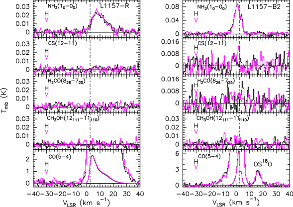
Figure 10: The NH₃, CS, H₂CO, CH₃OH, and CO transitions in L1557 positions (see Table 3). The WBS Horizontal (H) and Vertical (V) polarization spectra shown in black and magenta, respectively. Lower panels show also a zoom-in. Note that adjacent to CO (5–4) at B2, the OS¹⁸O 7(5,3)–6(4,2) transition (E${}_{\rm u}\sim$88 K, $\nu_{0}=$ 576.24058 GHz) is also indicated.

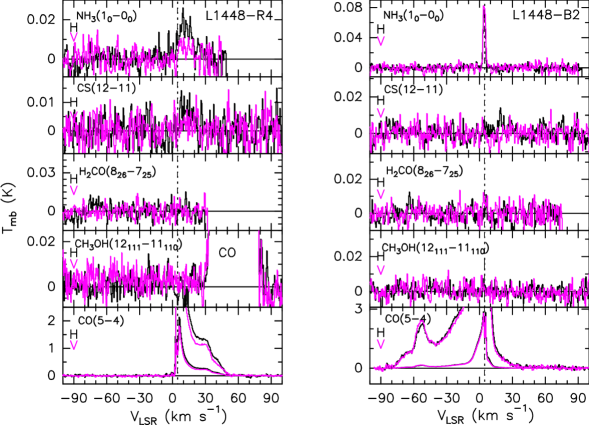
Figure 11: Same as Fig. 10 but for L1448 positions.

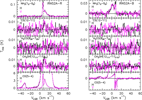
Figure 12: Same as Fig. 10 but for IRAS2a positions. Note that contamination from the image band of the CH₃OH 6(1, 6)–5(0, 5) transition (E${}_{\rm u}\sim$62 K, $\nu_{0}=$ 584.4499 GHz) is seen at V${}_{\rm lsr}\sim-$30 km s^-1.

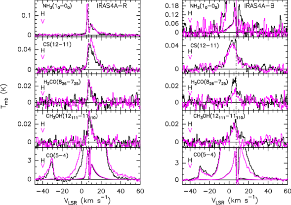
Figure 13: Same as Fig. 10 but for IRAS4a positions. Note that contamination from the image band of the CH₃OH 6(1, 6)–5(0, 5) transition (E${}_{\rm u}\sim$62 K, $\nu_{0}=$ 584.4499 GHz) is seen at V${}_{\rm lsr}\sim-$30 km s^-1.

Appendix B Column densities and NH₃ opacity calculations

We calculate the column densities of the observed species under the assumption of LTE and optically thin emission. The partition functions were calculated by using the standard assumptions (Turner, 1991) and with the molecular data taken from CDMS (Müller et al., 2005). The total integrated intensities reported in Table 4 are used. The following table shows the column densities for two temperatures, 20 K and 100 K.

Table 6: Column densities, from total integrated emission, assuming LTE and optically thin emission^a.

Position	o-NH3 (10–00)			CO (5–4) b			CH3OH (121,11–111,10)A+			p-H2CO (82,6–72,5)			CS (12–11)
	N(20)	N(100)		N(20)	N(100)		N(20)	N(100)		N(20)	N(100)		N(20)	N(100)
IRAS4A-B	1.3 1011	4.8 1011		6.5 1016	1.2 1016		7.4 1015	3.1 1013		9.1 1013	9.8 1011		5.2 1014	1.7 1012
IRAS4A-R	1.5 1011	5.6 1011		6.2 1016	1.1 1016		8.1 1015	3.4 1013		8.1 1013	8.7 1011		4.4 1014	1.4 1012
IRAS2A-B	5.4 1010	2.0 1011		1.2 1016	2.2 1015		–	–		–	–		–	–
IRAS2A-R	1.2 1011	4.5 1011		7.3 1016	1.3 1016		1.9 1015	7.8 1012		–	–		–	–
L1448-B2	4.1 1010	1.5 1011		7.0 1016	1.3 1016		–	–		–	–		–	–
L1448-R4	1.0 1010	3.8 1010		4.0 1016	7.3 1015		–	–		–	–		–	–
L1157-B2	9.0 1010	3.7 1011		4.8 1016	8.6 1015		–	–		–	–		–	–
L1157-R	5.4 1010	2.0 1011		4.8 1016	8.7 1015		–	–		–	–		–	–

^a The units are cm^-2, with N(20) and N(100) meaning the values obtained by assuming temperatures of 20 K and 100 K, respectively. ^b Due to effect of line absorption, this values should be considered as lower limits.

Using RADEX (van der Tak et al., 2007) we have computed the o-NH₃ (1₀–0₀) line opacity as a function of H₂ particle density. For the calculations we used an average linewidth of 10 km s^-1. The plots presented in Fig. 14 show the results for the column densities and temperatures values in Table 6. It is clear that in all cases $\tau$ $<<$ 1, also that $\tau$ is lower for higher H₂ particle density and kinetic temperature.

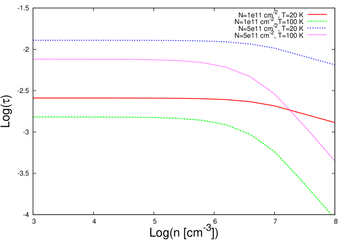
Figure 14: o-NH₃ (1₀–0₀) opacity as a function of H₂ particle density, from LVG calculations using RADEX. The different curves show different values of column density and kinetic temperature. Linewidth used in all cases is 10 km s^-1 (average observed linewidth).

References

- Bachiller & Cernicharo (1986) Bachiller R., Cernicharo J., 1986, A&A, 168, 262
- Bachiller et al. (1998) Bachiller R., Codella C., Colomer F., Liechti S., Walmsley C. M., 1998, A&A, 335, 266
- Bachiller & Perez Gutierrez (1997) Bachiller R., Perez Gutierrez M., 1997, ApJ, 487, L93+
- Bachiller et al. (2001) Bachiller R., Pérez Gutiérrez M., Kumar M. S. N., Tafalla M., 2001, A&A, 372, 899
- Ceccarelli et al. (2010) Ceccarelli C. et al., 2010, A&A, 521, L22
- Codella et al. (2010) Codella C. et al., 2010, A&A, 518, L112
- Curiel et al. (1999) Curiel S., Torrelles J. M., Rodríguez L. F., Gómez J. F., Anglada G., 1999, ApJ, 527, 310
- Draine, Roberge & Dalgarno (1983) Draine B. T., Roberge W. G., Dalgarno A., 1983, ApJ, 264, 485
- Garay et al. (1998) Garay G., Köhnenkamp I., Bourke T. L., Rodríguez L. F., Lehtinen K. K., 1998, ApJ, 509, 768
- Hirota et al. (2008) Hirota T. et al., 2008, PASJ, 60, 37
- Jiménez-Serra et al. (2008) Jiménez-Serra I., Caselli P., Martín-Pintado J., Hartquist T. W., 2008, A&A, 482, 549
- Jiménez-Serra et al. (2009) Jiménez-Serra I., Martín-Pintado J., Caselli P., Viti S., Rodríguez-Franco A., 2009, ApJ, 695, 149
- Jiménez-Serra et al. (2004) Jiménez-Serra I., Martín-Pintado J., Rodríguez-Franco A., Marcelino N., 2004, ApJ, 603, L49
- Jiménez-Serra et al. (2005) Jiménez-Serra I., Martín-Pintado J., Rodríguez-Franco A., Martín S., 2005, ApJ, 627, L121
- Jørgensen et al. (2007) Jørgensen J. K. et al., 2007, ApJ, 659, 479
- Kwon et al. (2006) Kwon W., Looney L. W., Crutcher R. M., Kirk J. M., 2006, ApJ, 653, 1358
- Lefloch et al. (2012) Lefloch B. et al., 2012, ApJ, 757, L25
- Looney, Mundy & Welch (2000) Looney L. W., Mundy L. G., Welch W. J., 2000, ApJ, 529, 477
- Looney, Tobin & Kwon (2007) Looney L. W., Tobin J. J., Kwon W., 2007, ApJ, 670, L131
- Menten et al. (2010) Menten K. M. et al., 2010, A&A, 521, L7
- Müller et al. (2005) Müller H. S. P., Schlöder F., Stutzki J., Winnewisser G., 2005, Journal of Molecular Structure, 742, 215
- Nisini et al. (2010) Nisini B. et al., 2010, A&A, 518, L120
- Nisini et al. (2013) Nisini B. et al., 2013, A&A, 549, A16
- Ott (2010) Ott S., 2010, in Astronomical Society of the Pacific Conference Series, Vol. 434, Astronomical Data Analysis Software and Systems XIX, Mizumoto Y., Morita K.-I., Ohishi M., eds., p. 139
- Rawlings et al. (1992) Rawlings J. M. C., Hartquist T. W., Menten K. M., Williams D. A., 1992, MNRAS, 255, 471
- Roelfsema et al. (2012) Roelfsema P. R. et al., 2012, A&A, 537, A17
- Santangelo et al. (2014) Santangelo G. et al., 2014, A&A, 568, A125
- Tafalla et al. (2013) Tafalla M. et al., 2013, A&A, 551, A116
- Turner (1991) Turner B. E., 1991, ApJ, 76, 617
- van der Tak et al. (2007) van der Tak F. F. S., Black J. H., Schöier F. L., Jansen D. J., van Dishoeck E. F., 2007, A&A, 468, 627
- van Dishoeck & Blake (1998) van Dishoeck E. F., Blake G. A., 1998, ARAA, 36, 317
- van Dishoeck et al. (2011) van Dishoeck E. F. et al., 2011, PASP, 123, 138
- Viti et al. (2004) Viti S., Collings M. P., Dever J. W., McCoustra M. R. S., Williams D. A., 2004, MNRAS, 354, 1141
- Viti et al. (2011) Viti S., Jimenez-Serra I., Yates J. A., Codella C., Vasta M., Caselli P., Lefloch B., Ceccarelli C., 2011, ApJ, 740, L3+
- Wakelam et al. (2005) Wakelam V., Ceccarelli C., Castets A., Lefloch B., Loinard L., Faure A., Schneider N., Benayoun J.-J., 2005, A&A, 437, 149