On the Optimality of Pseudo-polynomial Algorithms for Integer Programming

Abstract

In the classic Integer Programming (IP) problem, the objective is to decide whether, for a given $m\times n$ matrix $A$ and an $m$-vector $b=(b_{1},\dots,b_{m})$, there is a non-negative integer $n$-vector $x$ such that $Ax=b$. Solving (IP) is an important step in numerous algorithms and it is important to obtain an understanding of the precise complexity of this problem as a function of natural parameters of the input.

The classic pseudo-polynomial time algorithm of Papadimitriou [J. ACM 1981] for instances of (IP) with a constant number of constraints was only recently improved upon by Eisenbrand and Weismantel [SODA 2018] and Jansen and Rohwedder [ArXiv 2018]. We continue this line of work and show that under the Exponential Time Hypothesis (ETH), the algorithm of Jansen and Rohwedder is nearly optimal. We also show that when the matrix $A$ is assumed to be non-negative, a component of Papadimitriou’s original algorithm is already nearly optimal under ETH.

This motivates us to pick up the line of research initiated by Cunningham and Geelen [IPCO 2007] who studied the complexity of solving (IP) with non-negative matrices in which the number of constraints may be unbounded, but the branch-width of the column-matroid corresponding to the constraint matrix is a constant. We prove a lower bound on the complexity of solving (IP) for such instances and obtain optimal results with respect to a closely related parameter, path-width. Specifically, we prove matching upper and lower bounds for (IP) when the path-width of the corresponding column-matroid is a constant.

1 Introduction

In the classic Integer Programming problem, the input is an $m\times n$ integer matrix $A$, and an $m$-vector $b=(b_{1},\dots,b_{m})$. We consider the feasibility version of the problem, where the objective is to find a non-negative integer $n$-vector $x$ (if one exists) such that $Ax=b$. Solving this problem, denoted by (IP), is a fundamental step in numerous algorithms and it is important to obtain an understanding of the precise complexity of this problem as a function of natural parameters of the input.

(IP) is known to be NP-hard. However, there are two classic algorithms due to Lenstra [15] and Papadimitriou  [18] solving (IP) in polynomial or pseudo-polynomial time for two important cases when the number of variables and the number of constraints are bounded. These algorithms in some sense complement each other.

The algorithm of Lenstra shows that (IP) is solvable in polynomial time when the number of variables is bounded. Actually, the result of Lenstra is even stronger: (IP) is fixed-parameter tractable parameterized by the number of variables. However, the running time of Lenstra’s algorithm is doubly exponential in $n$. Later, Kannan [14] provided an algorithm for (IP) running in time $n^{{\mathcal{O}}(n)}$. Deciding whether the running time $n^{{\mathcal{O}}(n)}$ can be improved to $2^{{\mathcal{O}}(n)}$ is a long-standing open question.

Our work is motivated by the complexity analysis of the complementary case when the number of constraints is bounded. (IP) is NP-hard already for $m=1$ (the Knapsack problem) but solvable in pseudo-polynomial time. In 1981, Papadimitriou [18] extended this result by showing that (IP) is solvable in pseudo-polynomial time on instances for which the number of constraints $m$ is a constant. The algorithm of Papadimitriou consists of two steps. The first step is combinatorial, showing that if the entries of $A$ and $b$ are from $\{0,\pm 1,\dots,\pm d\},$ and (IP) has a solution, then there is also a solution which is in $\{0,1,\dots,n(md)^{2m+1}\}^{n}$. The second, algorithmic step shows that if (IP) has a solution with the maximum entry at most $B$, then the problem is solvable in time ${\mathcal{O}}((nB)^{m+1})$. Thus the total running time of Papadimitriou’s algorithm is ${\mathcal{O}}(n^{2m+2}\cdot(md)^{(m+1)(2m+1)})$, where $d$ is an upper bound on the absolute values of the entries of $A$ and $b$. There was no algorithmic progress on this problem until the very recent breakthrough of Eisenbrand and Weismantel [6]. They proved the following result.

Proposition (Theorem 2.2, Eisenbrand and Weismantel [6]).

(IP) with $m\times n$ matrix $A$ is solvable in time $(m\cdot\Delta)^{{\mathcal{O}}(m)}\cdot\|b\|_{\infty}^{2}$, where $\Delta$ is an upper bound on the absolute values of the entries of $A$.

Then, Jansen and Rohwedder improved Proposition 1 and gave a matching lower bound very recently [12].

Proposition (Jansen and Rohwedder [12]).

(IP) with $m\times n$ matrix $A$ is solvable in time ${\mathcal{O}}(m\Delta)^{m}\log(\Delta)\log(\Delta+\|b\|_{\infty})$. where $\Delta$ is an upper bound on the absolute values of the entries of $A$. Assuming the Strong Exponential Time Hypothesis (SETH), there is no algorithm for (IP) running in time $n^{{\mathcal{O}}(1)}\cdot{\mathcal{O}}(m(\Delta+\|b\|_{\infty}))^{m-\delta}$ for any $\delta>0$.

SETH is the hypothesis that CNF-SAT cannot be solved in time $(2-\epsilon)^{n}m^{{\mathcal{O}}(1)}$ on $n$-variable $m$-clause formulas for any constant $\epsilon$. ETH is the hypothesis that 3-SAT cannot be solved in time $2^{o(n)}$ on $n$-variable formulas. Both ETH and SETH were first introduced in the work of Impagliazzo and Paturi [10], which built upon earlier work of Impagliazzo, Paturi and Zane [11]. One of the natural question is whether the exponential dependence of $\|b\|_{\infty}$ can be improved significantly at the cost of super polynomial dependence on $n$. Our first theorem provides a conditional lower bound indicating that any significant improvements are unlikely.

Theorem 1.1.

Unless the Exponential Time Hypothesis (ETH) fails, (IP) with $m\times n$ matrix $A$ cannot be solved in time $n^{o(\frac{m}{\log m})}\cdot\|b\|_{\infty}^{o(m)}$ even when the constraint matrix $A$ is non-negative and each entry in any feasible solution is at most $2$.

Let us note that since the bound in Theorem 1.1 holds for a non-negative matrix $A$, we can always reduce (in polynomial time) the original instance of the problem to an equivalent instance where the maximum value $\Delta$ in the constraint matrix $A$ does not exceed $\|b\|_{\infty}$. Thus Theorem 1.1 also implies the conditional lower bound $n^{o(\frac{m}{\log m})}\cdot(\Delta\cdot\|b\|_{\infty})^{o(m)}$. When $m={\mathcal{O}}(n)$, our bound also implies the lower bound $(n\cdot m)^{o(\frac{m}{\log m})}\cdot(\Delta\cdot\|b\|_{\infty})^{o(m)}$. We complement Theorem 1.1 by turning our focus to the dependence of algorithms solving (IP) on $m$ alone, and obtaining the following theorem.

Theorem 1.2.

Unless the Exponential Time Hypothesis (ETH) fails, (IP) with $m\times n$ matrix $A$ cannot be solved in time $f(m)\cdot(n\cdot\|b\|_{\infty})^{o(\frac{m}{\log m})}$ for any computable function $f$. The result holds even when the constraint matrix $A$ is non-negative and each entry in any feasible solution is at most $1$.

The difference between our first two theorems is the following. Although Theorem 1.1 provides a better dependence on $\|b\|_{\infty}$, Theorem 1.2 provides much more information on how the complexity of the problem depends on $m$. Since several parameters are involved in this running time estimation, a natural objective is to study the possible tradeoffs between them. For instance, consider the ${\mathcal{O}}(m\Delta)^{m}\log(\Delta)\log(\Delta+\|b\|_{\infty})$ time algorithm (Proposition 1) for (IP). A natural follow up question is the following. Could it be that by allowing a significantly worse dependence (a superpolynomial dependence) on $n$ and $\|b\|_{\infty}$ and an arbitrary dependence on $m$, one might be able to improve the dependence on $\Delta$ alone? Theorem 1.2 provides a strong argument against such an eventuality. Indeed, since the lower bound of Theorem 1.2 holds even for non-negative matrices, it rules out algorithms with running time $f(m)\cdot\Delta^{o(\frac{m}{\log m})}\cdot(n\cdot\|b\|_{\infty})^{o(\frac{m}{\log m})}$. Therefore, obtaining a subexponential dependence of $\Delta$ on ${m}$ even at the cost of a superpolynomial dependence of $n$ and $\|b\|_{\infty}$ on $m$, and an arbitrarily bad dependence on $m$ is as hard as obtaining a subexponential algorithm for 3-SAT.

We now motivate our remaining results. We refer the reader to Figure 1 for a summary of our main results. It is straightforward to see that when the matrix $A$ happens to be non-negative, the algorithm of Papadimitriou [18] runs in time ${\mathcal{O}}((n\cdot\|b\|_{\infty})^{m+1})$. Due to Theorems 1.1 and  1.2, the dynamic programming step of the algorithm of Papadimitriou for (IP) when the maximum entry in a solution as well as in the constraint matrix is bounded, is already close to optimal. Consequently, any quest for “faster” algorithms for (IP) must be built around the use of additional structural properties of the matrix $A$. Cunningham and Geelen [1] introduced such an approach by considering the branch decomposition of the matrix $A$. They were motivated by the fact that the result of Papadimitriou can be interpreted as a result for matrices of constant rank and branch-width is a parameter which is upper bounded by rank plus one. For a matrix $A$, the column-matroid of $A$ denotes the matroid whose elements are the columns of $A$ and whose independent sets are precisely the linearly independent sets of columns of $A$. We postpone the formal definitions of branch decomposition and branch-width till the next section. For (IP) with a non-negative matrix $A$, Cunningham and Geelen [1] showed that when the branch-width of the column-matroid of $A$ is constant, (IP) is solvable in pseudo-polynomial time.

Proposition 1.3 (Cunningham and Geelen [1]).

(IP) with a non-negative $m\times n$ matrix $A$ given together with a branch decomposition of its column matroid of width $k$, is solvable in time ${\mathcal{O}}((\|b\|_{\infty}+1)^{2k}mn+m^{2}n)$.

We analyze the complexity of (IP) parameterized by the branch-width of $A$, by making use of SETH and obtain the following lower bound(s).

Theorem 1.4.

Unless SETH fails, (IP) with a non-negative $m\times n$ constraint matrix $A$ cannot be solved in time $f({\sf bw})(\|b\|_{\infty}+1)^{(1-\epsilon){\sf bw}}(mn)^{{\mathcal{O}}(1)}$ or $f(\|b\|_{\infty})(\|b\|_{\infty}+1)^{(1-\epsilon){\sf bw}}(mn)^{{\mathcal{O}}(1)}$, for any computable function $f$. Here $\sf bw$ is the branchwidth of the column matroid of $A$.

In recent years, SETH has been used to obtain several tight conditional bounds on the running time of algorithms for various optimization problems on graphs of bounded treewidth  [16]. However, in order to be able to use SETH to prove lower bounds for (IP) in combination with the branch-width of matroids, we have to develop new ideas.

In fact, Theorem 1.4 follows from stronger lower bounds we prove using the path-width of $A$ as our parameter of interest instead of the branch-width. The parameter path-width is closely related to the notion of trellis-width of a linear code, which is a parameter commonly used in coding theory [9]. For a matrix $A\in{\mathbb{R}}^{m\times n}$, computing the path-width of the column matroid of $A$ is equivalent to computing the trellis-width of the linear code generated by $A$. Roughly speaking, the path-width of the column matroid of $A$ is at most $k$, if there is a permutation of the columns of $A$ such that in the matrix $A^{\prime}$ obtained from $A$ by applying this column-permutation, for every $1\leq i\leq n-1$, the dimension of the subspace of ${\mathbb{R}}^{m}$ obtained by taking the intersection of the subspace of ${\mathbb{R}}^{m}$ spanned by the first $i$ columns with the subspace of ${\mathbb{R}}^{m}$ spanned by the remaining columns, is at most $k-1$.

Upper Bounds	Lower bounds
	no $n^{o(\frac{m}{\log m})}\cdot\|b\|_{\infty}^{o(m)}$ time algorithm under ETH (Theorem 1.1)
	(even for non-negative matrix $A$ and solution entries bounded by 2)
$(m\cdot\Delta)^{{\mathcal{O}}(m)}\cdot\|b\|_{\infty}^{{\mathcal{O}}(1)}$ [6, 12]	no $n^{{\mathcal{O}}(1)}\cdot{\mathcal{O}}(m(\Delta+\|b\|_{\infty}))^{m-\delta}$ time algorithm for $\delta>0$ under SETH [12]
	no $(n\cdot m)^{o(\frac{m}{\log m})}(\Delta\cdot\|b\|_{\infty})^{o(m)}$ algorithm when $m={\mathcal{O}}(n)$ under ETH
	(consequence of Theorem 1.1)
	(even for non-negative matrix $A$ and solution entries bounded by 2)
	no $f(m)\cdot(n\cdot\|b\|_{\infty})^{o(\frac{m}{\log m})}$ under ETH (Theorem 1.2)
	(even for non-negative matrix $A$ and solution entries bounded by 1)
${\mathcal{O}}((\|b\|_{\infty}+1)^{{\sf pw}+1}mn+m^{2}n)$	no $f({\sf pw})(\|b\|_{\infty}+1)^{(1-\epsilon){\sf pw}}(mn)^{{\mathcal{O}}(1)}$ algorithm under SETH (Theorem 1.5)
(non-negative matrix $A$)	(even for non-negative matrix $A$)
(Theorem 1.7)
	no $f(\|b\|_{\infty})(\|b\|_{\infty}+1)^{(1-\epsilon){\sf pw}}(mn)^{{\mathcal{O}}(1)}$ algorithm under SETH (Theorem 1.6)
	(even for non-negative matrix $A$)
${\mathcal{O}}((\|b\|_{\infty}+1)^{2{\sf bw}}mn+m^{2}n)$	no $f({\sf bw})(\|b\|_{\infty}+1)^{(1-\epsilon){\sf bw}}(mn)^{{\mathcal{O}}(1)}$
(non-negative matrix $A$) [1]	or
	$f(\|b\|_{\infty})(\|b\|_{\infty}+1)^{(1-\epsilon){\sf bw}}(mn)^{{\mathcal{O}}(1)}$ algorithm
	under SETH (Theorem 1.4)
	(even for non-negative matrix $A$)

Figure 1: A summary of our lower bound results in comparison with the relevant known upper bound results. Here, $n$ and $m$ are the number of variables and constraints respectively, ${\sf pw}$ and ${\sf bw}$ denote the path-width and branch-width of the column matroid of $A$ and $\|b\|_{\infty}$ denotes a bound on the largest absolute value in $b$ while $\Delta$ denotes a bound on the largest absolute value in $A$.

The value of the parameter path-width is always at least the value of branch-width and thus Theorem 1.4 follows from the following theorems.

Theorem 1.5.

Unless SETH fails, (IP) with even a non-negative $m\times n$ constraint matrix $A$ cannot be solved in time $f(k)(\|b\|_{\infty}+1)^{(1-\epsilon)k}(mn)^{{\mathcal{O}}(1)}$ for any computable function $f$ and $\epsilon>0$, where $k$ is the path-width of the column matroid of $A$.

Theorem 1.6.

Unless SETH fails, (IP) with even a non-negative $m\times n$ constraint matrix $A$ cannot be solved in time $f(\|b\|_{\infty})(\|b\|_{\infty}+1)^{(1-\epsilon)k}(mn)^{{\mathcal{O}}(1)}$ for any computable function $f$ and $\epsilon>0$, where $k$ is the path-width of the column matroid of $A$.

Although the proofs of both lower bounds have a similar structure, we believe that there are sufficiently many differences in the proofs to warrant stating and proving them separately.

Note that although there is still a gap between the upper bound of Cunningham and Geelen from Proposition 1.3 and the lower bound provided by Theorem 1.4, the lower bounds given in Theorems 1.6 and 1.5 are asymptotically tight in the following sense. The proof of Cunningham and Geelen in [1] actually implies the upper bound stated in Theorem 1.7. We provide a self-contained proof in this paper for the reader’s convenience.

Theorem 1.7.

(IP) with non-negative $m\times n$ matrix $A$ given together with a path decomposition of its column matroid of width $k$ is solvable in time ${\mathcal{O}}((\|b\|_{\infty}+1)^{k+1}mn+m^{2}n)$.

Then by Theorem 1.5, we cannot relax the $(\|b\|_{\infty}+1)^{k}$ factor in Theorem 1.7 even if we allow in the running time an arbitrary function depending on $k$, while Theorem 1.6 shows a similar lower bound in terms of $\|b\|_{\infty}$ instead of $k$. Put together the results imply that no matter how much one is allowed to compromise on either the path-width or the bound on $\|b\|_{\infty}$, it is unlikely that the algorithm of Theorem 1.7 can be improved.

The path-width of matrix $A$ does not exceed its rank and thus the number of constraints in (IP). Hence, similar to Proposition 1.3, Theorem 1.7 generalizes the result of Papadimitriou when restricted to non-negative matrices. Also we note that the assumption of non-negativity is unavoidable (without any further assumptions such as a bounded domain for the variables) in this setting because (IP) is NP-hard when the constraint matrix $A$ is allowed to have negative values (in fact even when restricted to $\{-1,0,1\}$) and the branchwidth of the column matroid of $A$ is at most 3. A close inspection of the instances they construct in their NP-hardness reduction shows that the column matroids of the resulting constraint matrices are in fact direct sums of circuits, implying that even their path-width is bounded by 3.

Organization of the paper. The rest of the paper is organized as follows. There are two main technical parts to this paper. The first part (Section 3) is devoted to proving Theorem 1.1 and Theorem 1.2 (our ETH based lower bounds) while the second part (Section 4) is devoted to proving Theorem 1.5 and Theorem 1.6 (our SETH based lower bounds), and consequently, Theorem 1.4. For all our reductions, we begin by giving an overview in order to help the reader (especially in the SETH based reductions) navigate the technical details in the reductions. We then prove Theorem 1.6 in Section 4.3 and Theorem 1.7 in Section 5 (completing the results for constant path-width).

2 Preliminaries

We assume that the reader is familiar with basic definitions from linear algebra, matroid theory and graph theory.

Notations. We use ${\mathbb{Z}}_{\scriptscriptstyle{\geq 0}}$ and ${\mathbb{R}}$ to denote the set of non negative integers and real numbers, respectively. For any positive integer $n$, we use $[n]$ and $\mathbb{Z}_{n}$ to denotes the sets $\{1,\ldots,n\}$ and $\{0,1,\ldots,n-1\}$, respectively. For convenience, we say that $[0]=\emptyset$. For any two vectors $b,b^{\prime}\in{\mathbb{R}}^{m}$ and $i\in[m]$, we use $b[i]$ to denote the $i^{th}$ coordinate of $b$ and we write $b^{\prime}\leq b$, if $b^{\prime}[i]\leq b[i]$ for all $i\in[m]$. We often use $0$ to denote the zero-vector whose length will be clear from the context. For a matrix $A\in{\mathbb{R}}^{m\times n}$, $I\subseteq[m]$ and $J\subseteq[n]$, $A[I,J]$ denote the submatrix of $A$ obtained by the restriction of $A$ to the rows indexed by $I$ and columns indexed by $J$. For an $m\times n$ matrix $A$ and $n$-vector $v$, we can write $Av=\sum_{i=1}^{n}A_{i}v[i]$, where $A_{i}$ is the $i^{th}$ column of $A$. Here we say that $v[i]$ is a multiplier of column $A_{i}$. For convenience, in this paper, we consider $0$ as an even number.

Branch-width of matroids. The notion of the branch-width of graphs, and implicitly of matroids, was introduced by Robertson and Seymour in [19]. Let ${M}=(U,{\cal F})$ be a matroid with universe set $U$ and family ${\cal F}$ of independent sets over $U$. We use $r_{M}$ to denote the rank function of $M$. That is, for any $S\subseteq U$, $r_{M}(S)=\max_{S^{\prime}\subseteq S,S^{\prime}\in{\cal F}}|S^{\prime}|$. For $X\subseteq U$, the connectivity function of $M$ is defined as

$$\lambda_{M}(X)=r_{M}(X)+r_{M}(U\setminus X)-r_{M}(U)+1$$

For matrix $A\in{\mathbb{R}}^{m\times n}$, we use $M(A)$ to denote the column-matroid of $A$. In this case the connectivity function $\lambda_{M(A)}$ has the following interpretation. For $E=\{1,\dots,n\}$ and $X\subseteq E$, we define

$$S(A,X)=\operatorname{span}(A|X)\cap\operatorname{span}(A|E\setminus X),$$

where $A|X$ is the set of columns of $A$ restricted to $X$ and $\operatorname{span}(A|X)$ is the subspace of ${\mathbb{R}}^{m}$ spanned by the columns $A|X$. It is easy to see that the dimension of $S(A,X)$ is equal to $\lambda_{M(A)}(X)-1$.

A tree is cubic if its internal vertices all have degree $3$. A branch decomposition of matroid ${M}$ with universe set $U$ is a cubic tree $T$ and mapping $\mu$ which maps elements of $U$ to leaves of $T$. Let $e$ be an edge of $T$. Then the forest $T-e$ consists of two connected components $T_{1}$ and $T_{2}$. Thus every edge $e$ of $T$ corresponds to the partitioning of $U$ into two sets $X_{e}$ and $U\setminus X_{e}$ such that $\mu(X_{e})$ are the leaves of $T_{1}$ and $\mu(U\setminus X_{e})$ are the leaves of $T_{2}$. The width of edge $e$ is $\lambda_{M}(X_{e})$ and the width of branch decomposition $(T,\mu)$ is the maximum edge width, where maximum is taken over all edges of $T$. Finally, the branch-width of $M$ is the minimum width taken over all possible branch decompositions of $M$.

The path-width of a matroid is defined as follows. Recall that a caterpillar is a tree which is obtained from a path by attaching leaves to some vertices of the path. Then the path-width of a matroid is the minimum width of a branch decomposition $(T,\mu)$, where $T$ is a cubic caterpillar. Let us note that every mapping of elements of a matroid to the leaves of a cubic caterpillar corresponds to an ordering of these elements. Jeong, Kim, and Oum [13] gave a constructive fixed-parameter tractable algorithm to construct a path decomposition of width at most $k$ for a column matroid of a given matrix.

ETH and SETH. For $q\geq 3$, let $\delta_{q}$ be the infimum of the set of constants $c$ for which there exists an algorithm solving $q$-SAT with $n$ variables and $m$ clauses in time $2^{cn}\cdot m^{{\mathcal{O}}(1)}$. The Exponential-Time Hypothesis (ETH) and Strong Exponential-Time Hypothesis (SETH) are then formally defined as follows. ETH conjectures that $\delta_{3}>0$ and SETH that $\lim_{q\to\infty}\delta_{q}=1$.

3 ETH lower bounds on pseudopolynomial solvability of (IP)

In this section we prove Theorems 1.1 and 1.2.

3.1 Proof of Theorem 1.1

This subsection is devoted to the proof of Theorem 1.1

See 1.1

Our proof is by a reduction from $3$-CNF SAT to (IP). There are exactly 2 variables in the (IP) instance for each variable (one for each literal) and clause. For each clause we define two constraints. For each variable in the 3-CNF formula, we have a constraint, which is a selection gadget.

	${x_{1}}$	${\bar{x}_{1}}$	${x_{2}}$	${\bar{x}_{2}}$	${x_{3}}$	${\bar{x}_{3}}$	${x_{4}}$	${\bar{x}_{4}}$	${Y_{1}}$	${Z_{1}}$	${Y_{2}}$	${Z_{2}}$	${Y_{3}}$	${Z_{3}}$
$C_{1}$	1	0	1	0	1	0	0	0	1
									1	1
$C_{2}$	0	1	0	1	1	0	0	0			1
											1	1
$C_{3}$	0	0	0	1	0	1	0	1					1
													1	1
$x_{1}$	1	1
$x_{2}$			1	1
$x_{3}$					1	1
$x_{4}$							1	1

Figure 2: An illustration of the matrix $A_{\psi}$ corresponding to the 3-CNF formula $\psi=(x_{1}\vee x_{2}\vee x_{3})\wedge(\bar{x}_{1}\vee\bar{x}_{2}\vee x_{3})\wedge(\bar{x}_{4}\vee\bar{x}_{2}\vee\bar{x}_{3})$. The unfilled cells have 0 as the entry.

We now proceed to the formal description of the reduction. From a $3$-CNF formula $\psi$ on $n$ variables and $m$ clauses we create an equivalent (IP) instance $A_{\psi}x=b_{\psi},x\geq 0$, where $A_{\psi}$ is a non-negative integer $(2m+n)\times 2(m+n)$ matrix and the largest entry in $b_{\psi}$ is $3$. Our reduction can be easily seen to be a polynomial time reduction and we do not give an explicit analysis. Let $\psi$ be the input of $3$-CNF SAT. Let $X=\{x_{1},\ldots,x_{n}\}$ be the set of variables in $\psi$ and ${\mathcal{C}}=\{C_{1},\ldots,C_{m}\}$ be the set of clauses in $\psi$. First we define the set of variables in the in the (IP) instance. For each $x_{i}\in X$, we have two variables $x_{i}$ and $\overline{x}_{i}$ in the (IP) instance $A_{\psi}x=b_{\psi},x\geq 0$. For each $C_{i}\in{\mathcal{C}}$, we have two variables $Y_{i}$ and $Z_{i}$.

Now we define the set of constraints of $A_{\psi}x=b_{\psi},x\geq 0$. For each $C_{i}=x\vee y\vee z$, we define two constraints

$$x+y+z+Y_{i} = 3\qquad\mbox{and}$$ (1)

$$Y_{i}+Z_{i} = 2.$$ (2)

$$\mbox{For each $i\in[n]$,}\qquad\qquad x_{i}+\overline{x}_{i}=1$$ (3)

This completes the construction of (IP) instance $A_{\psi}x=b_{\psi},x\geq 0$. See Figure 2 for an illustration. We now argue that this reduction correctly maps satisfiable 3-CNF formulas to feasible instances of (IP) and vice versa.

Lemma 3.1.

The formula $\psi$ is satisfiable if and only if $A_{\psi}x=b_{\psi},x\geq 0$ is feasible.

Proof 3.2.

Suppose that the formula $\psi$ is satisfiable and let $\phi$ be a satisfying assignment of $\psi$. We set values for the variables $\{x_{i},\overline{x}_{i}\colon i\in[n]\}\cup\{Y_{i},Z_{i}\colon i\in[m]\}$ and prove that $A_{\psi}x=b_{\psi}$. For any $i\in[n]$, if $\phi(x_{i})=1$ we set $x_{i}=1$ and $\overline{x}_{i}=0$. Otherwise, we set $x_{i}=0$ and $\overline{x}_{i}=1$.

For every $i\in[m]$, we define

$$Y_{i}=\left\{\begin{array}[]{ll}0&\mbox{if the number of literals set to $1$ in $C_{i}$ by $\phi$ is $3$,}\\ 1&\mbox{if the number of literals set to $1$ in $C_{i}$ by $\phi$ is $2$,}\\ 2&\mbox{otherwise,}\end{array}\right.$$ (4)

and

$$Z_{i}=\left\{\begin{array}[]{ll}2&\mbox{if the number of literals set to $1$ in $C_{i}$ by $\phi$ is $3$,}\\ 1&\mbox{if the number of literals set to $1$ in $C_{i}$ by $\phi$ is $2$,}\\ 0&\mbox{otherwise.}\end{array}\right.$$ (5)

We now proceed to prove that the above substitution of values to the variables is indeed a feasible solution. Towards this, we need to show that (1), (2), and (3) are satisfied. First consider (1). Let $C_{i}=x\vee y\vee z$. Since $\phi$ is a satisfying assignment, we have that $1\leq x+y+z\leq 3$. Thus, by (4), we conclude that $x+y+z+Y_{i}=3$. Because of (4) and (5), (2) is satisfied. Since the values for $\{x_{i},\overline{x}_{i}\colon i\in[n]\}$ is derived from an assignment $\phi$, (3) is satisfied.

For the converse direction of the statement of the lemma, suppose that there exists non-negative values for the set of variables $\{x_{i},\overline{x}_{i}\colon i\in[n]\}\cup\{Y_{i},Z_{i}\colon i\in[m]\}$, such that (1), (2), and (3) are satisfied. Now we need to show that $\psi$ is satisfiable. Because of (3), we know that exactly one of $x_{i}$ and $\overline{x}_{i}$ is set to one and other is set to zero. Next, we define an assignment $\phi$ and prove that $\phi$ is a satisfying assignment for $\psi$. For $i\in[n]$ we define

$$\phi(x_{i})=\left\{\begin{array}[]{ll}1&\mbox{if }x_{i}=1,\\ 0&\mbox{if }\overline{x}_{i}=1.\end{array}\right.$$

We claim that $\phi$ satisfies all the clauses. Consider a clause $C_{j}=x\vee y\vee z$ where $j\in[m]$. Since $Y_{j}+Z_{j}=2$ (by (2)), we have that $Y_{i}\in\{0,1,2\}$. Since $Y_{i}\in\{0,1,2\}$, by (1), at least one of $x,y$ or $z$ is set to one. This implies that $\phi$ satisfies $C_{j}$. This completes the proof of the lemma.

By (2) and (3), we have that the value set for any variable in a feasible solution is at most $2$. The following lemma completes the proof of the theorem.

Lemma 3.3.

If there is an algorithm for (IP) running in time $n^{o(\frac{m}{\log m})}\|b\|_{\infty}^{o(m)}$, then ETH fails.

Proof 3.4.

By the Sparsification Lemma [11], we know that $3$-CNF SAT on $n^{\prime}$ variables and $cn^{\prime}$ clauses, where $c$ is a constant, cannot be solved in time $2^{o(n^{\prime})}$ time. Suppose there is an algorithm ALG for (IP) running in time $n^{o(\frac{m}{\log m})}\|b\|_{\infty}^{o(m)}$. Then for a $3$-CNF formula $\psi$ with $n^{\prime}$ variables and $m^{\prime}=cn$ clauses we create an instance $A_{\psi}x=b_{\psi},$ $x\geq 0$ of (IP) as discussed in this section, in polynomial time, where $A_{\psi}$ is a matrix of dimension $(2cn^{\prime}+n^{\prime})\times(2(n^{\prime}+cn^{\prime}))$ and the largest entry in $b_{\psi}$ is $3$. Then by Lemma 3.1, we can run ALG to test whether $\psi$ is satisfiable or not. This takes time

$$(2(cn^{\prime}+n^{\prime}))^{o(\frac{2cn^{\prime}+n^{\prime})}{\log(2cn^{\prime}+n^{\prime})})}\cdot 3^{o(2cn^{\prime}+n^{\prime})}=2^{o(n^{\prime})},$$

hence refuting ETH.

3.2 Proof of Theorem 1.2

In this section we prove the following theorem.

See 1.2

Towards proving Theorem 1.2 we use the ETH based lower bound result of Marx [17] for Partitioned Subgraph Isomorphism. For two graphs $G$ and $H$, a map $\phi\colon V(G)\mapsto V(H)$ is called a subgraph isomorphism from $G$ to $H$, if $\phi$ is injective and for any $\{u,v\}\in E(G)$, $\{\phi(u),\phi(v)\}\in E(H)$ (see Figure 3 for an illustration).

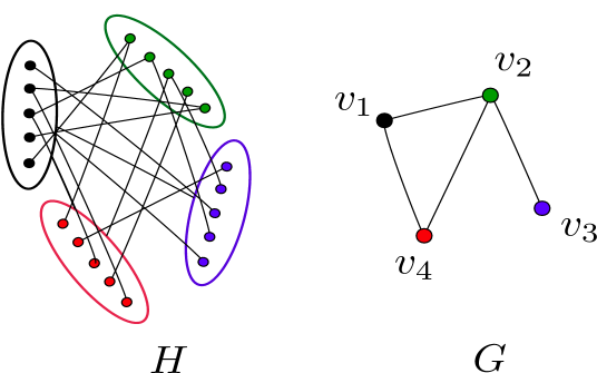
Figure 3: An illustration of an instance of Partitioned Subgraph Isomorphism.

Partitioned Subgraph Isomorphism Input: Two graphs $G,H$, a bijection $c_{G}\colon V(G)\mapsto[\ell]$ and a function $c_{H}\colon V(H)\mapsto[\ell]$, where $\ell=|V(G)|$. Question: Is there a subgraph isomorphism $\phi$ from $G$ to $H$ such that for any $v\in V(G)$, $c_{G}(v)=c_{H}(\phi(v))$?

Lemma 3.5 (Corollary 6.3 [17]).

If Partitioned Subgraph Isomorphism can be solved in time $f(G)n^{o(\frac{k}{\log k})}$, where $f$ is an arbitrary function, $n=|V(H)|$ and $k$ is the number of edges of the smaller graph $G$, then ETH fails.

To prove Theorem 1.2 we give a polynomial time reduction from Partitioned Subgraph Isomorphism to (IP) such that for every instance $(G,H,c_{G},c_{H})$ of Partitioned Subgraph Isomorphism  the reduction outputs an instance of (IP) where the constraint matrix has dimension ${\mathcal{O}}(|E(G)|)\times{\mathcal{O}}(|E(H)|)$ and the largest value in the target vector is $\max\{|E(H)|,|V(H)|\}$.

Let $(G,H,c_{G},c_{H})$ be an instance of Partitioned Subgraph Isomorphism. Let $k=|E(G)|$ and $n=|V(H)|$. We construct an instance $Ax=b$ of (IP) from $(G,H,c_{G},c_{H})$ in polynomial time. Without loss of generality we assume that $[n]=V(H)$ and that there are no isolated vertices in $G$. Hence, the number of vertices in $G$ is at most $2k$. Let $m=|E(H)|$. For each $e\in E(H)$ we assign a unique integer from $[m]$. Let $\alpha\colon E(H)\mapsto[m]$ be the bijection which represents the assignment mentioned above. For any $i,j\in[\ell]$, we use $E_{H}(i,j)$ as a shorthand for the set of edges of $H$ between $c_{H}^{-1}(i)$ and $c_{H}^{-1}(j)$. Finally, for ease of presentation we let $\{v_{1},\ldots,v_{\ell}\}=V(G)$ and $c_{G}(v_{i})=i$ for all $i\in[\ell]$, where $\ell=|V(G)|$.

For illustrative purposes, before proceeding to the formal construction, we give an informal description of the (IP) instance we obtain from a specific instance of Partitioned Subgraph Isomorphism. Let $H$ and $G$ be the graphs in Figure 3 and consider the graph $\widehat{H}$ obtained from $H$ as depicted in Figure 4.

For every color $i\in[\ell]$ we have a column in $\widehat{H}$ and for every pair of distinct colors $i,j\in[\ell]$ such that $\{v_{i},v_{j}\}\in E(G)$, we have a copy of $c_{H}^{-1}(i)$ in Column $i$ and Row $i$ and a copy of $c_{H}^{-1}(i)$ in Column $i$ and Row $j$. Thus, Column $i$ comprises at most $\ell$ copies of the vertices of $H$ whose image under $c_{H}$ is $i$ and Row $i$ comprises a copy of $c_{H}^{-1}(i)$ and additionally, a copy of every vertex $u$ of $H$ such that $v_{c_{H}{u}}$ is adjacent to $v_{i}$ in $G$. That is, the color of $u$ is “adjacent” to the color $i$ in $G$.

For a vertex $u\in V(H)$, we refer to the unique copy of $u$ in the $i^{th}$ row as the $i^{th}$ copy of $u$ in $\widehat{H}$. For every edge $e=\{a,b\}\in E(H)$ where $c_{H}(a)=i$, $c_{H}(b)=j$, and $\{v_{i},v_{j}\}\in E(G)$, we have two copies of $e$ in $\widehat{H}$. The first copy of $e$ has as its endpoints, the $i^{th}$ copy of $a$ and the $i^{th}$ copy of $b$ and the second copy of $e$ has as its endpoints, the $j^{th}$ copy of $a$ and the $j^{th}$ copy of $b$. We now rephrase the Partitioned Subgraph Isomorphism problem (informally) as a problem of finding a certain type of subgraph in $\widehat{H}$, which in turn will point us in the direction of our (IP) instance in a natural way. The rephrased problem statement is the following. Given $G$, $H$,$c_{H}$,$c_{G}$ and the resulting auxiliary graph $\widehat{H}$, find a set of $2|E(H)|$ edges in $\widehat{H}$ such that the following properties hold.

• (Selection) For every $\{v_{i},v_{j}\}\in E(G)$, we pick a unique edge in $\widehat{H}$ with one endpoint in (Row $i$, Column $i$) and the other endpoint in (Row $i$, Column $j$) and we pick a unique edge with one endpoint in (Row $j$, Column $j$) and the other endpoint in (Row $j$, Column $i$).

• (Consistency 1) All the edges we pick from Row $i$ of $\widehat{H}$ share a common endpoint at the position (Row $i$, Column $i$).

• (Consistency 2) For any edge $e=\{a,b\}\in E(H)$ such that $c_{H}(a)=i$, $c_{H}(b)=j$, if the copy of $e$ in Row $i$ is selected in our solution then our solution contains the copy of $e$ in Row $j$ as well.

It is straightforward to see that a set of edges of $\widehat{H}$ which satisfy the stated properties imply a solution to our Partitioned Subgraph Isomorphism instance in an obvious way. In order to obtain our (IP) instance, we create a variable for every edge in $\widehat{H}$ (or 2 for every edge in $E(H)$) and encode the properties stated above in the form of constraints. We now formally define the (IP) instance output by our reduction.

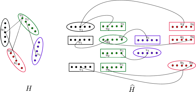
Figure 4: An illustration of the auxiliary graph $\widehat{H}$ capturing the representation of the vertices and some edges of $H$.

The set of indeterminants $x$ of the (IP) instance is

$$\left\{x(\{a,b\},c_{H}(a),c_{H}(b))\colon\{a,b\}\in E(H)\right\}.$$

Notice that for any $\{a,b\}\in E(H)$, there exist an associated pair of indeterminants, namely $x(\{a,b\},c_{H}(a),c_{H}(b))$ and $x(\{a,b\},c_{H}(b),c_{H}(a))$. Thus the cardinality of $x$ is upper bounded by $2|E(H)|=2m$. Recall that $\{v_{1},\ldots,v_{\ell}\}=V(G)$ and $c_{G}(v_{i})=i$ for all $i\in[\ell]$, where $\ell=|V(G)|$. For each $v_{i}\in V(G)$ we define $2d_{G}(v_{i})-1$ many constraints as explained below. Let $r=d_{G}(v_{i})$ and $N_{G}(v_{i})=\{v_{j_{1}},\ldots,v_{j_{r}}\}$. The constraints for $v_{i}\in V(G)$ are the following. For all $q\in[r]$,

$$\sum_{\begin{subarray}{c}e\in E_{H}(i,j_{q})\end{subarray}}x(e,i,j_{q})=1$$ (6)

The constraints of the form above enforce the (Selection) property described in our informal summary.

For all $q\in[r-1]$,

$$\sum_{\begin{subarray}{c}\{a,b\}\in E_{H}(i,j_{q})\\ a\in c_{H}^{-1}(i)\end{subarray}}a\cdot x(\{a,b\},i,j_{q})+\sum_{\begin{subarray}{c}\{a,b^{\prime}\}\in E_{H}(i,j_{q+1})\\ a\in c_{H}^{-1}(i)\end{subarray}}(n-a)\cdot x(\{a,b^{\prime}\},i,j_{q+1})=n$$ (7)

The constraints of the form above together enforce the (Consistency 1) property described in our informal summary.

For each $\{v_{i},v_{j}\}\in E(G)$ with $i<j$, we define the following constraint in the (IP) instance.

$$\sum_{\begin{subarray}{c}\{a,b\}\in E_{H}(i,j)\\ a\in c_{H}^{-1}(i)\end{subarray}}\alpha(\{a,b\})\cdot x(\{a,b\},i,j)+\sum_{\begin{subarray}{c}\{a,b\}\in E_{H}(i,j)\\ b\in c_{H}^{-1}(j)\end{subarray}}(m-\alpha(\{a,b\}))\cdot x(\{a,b\},j,i)=m$$ (8)

The constraints of the form above together enforce the (Consistency 2) property described in our informal summary.

This completes the construction of the (IP) instance $Ax=b,x\geq 0$. Notice that the construction of instance $Ax=b,x\geq 0$ can be done in polynomial time. Clearly, the number of rows in $A$ is $|E(G)|+\sum_{v\in V(G)}2d_{G}(v)-1\leq 5k$ and number of columns in $A$ is $2m$. Now we prove the correctness of the reduction.

Lemma 3.6.

$(G,H,c_{G},c_{H})$ is a Yes instance of Partitioned Subgraph Isomorphism if and only if $Ax=b,x\geq 0$ is feasible. Moreover, if $Ax=b,x\geq 0$ is feasible, then for any solution $x^{*}$, each entry of $x^{*}$ belongs to $\{0,1\}$.

Proof 3.7.

Suppose $(G,H,c_{G},c_{H})$ is a Yes instance of Partitioned Subgraph Isomorphism. Let $\phi\colon V(G)\mapsto V(H)$ be a solution to $(G,H,c_{G},c_{H})$. Now we define a solution $x^{*}\in\{0,1\}^{2m}$ to the instance $Ax=b,x\geq 0$ of (IP). We know that for each edge $\{v_{i},v_{j}\}\in E(G)$, $\{\phi(v_{i}),\phi(v_{j})\}\in E(H)$. For each edge $\{v_{i},v_{j}\}\in E(G)$, we set $x^{*}(\{\phi(v_{i}),\phi(v_{j})\},i,j)=x^{*}(\{\phi(v_{i}),\phi(v_{j})\},j,i)=1$. For every other indeterminant, we set its value to $0$. Now we prove that $Ax^{*}=b$.

Towards that first consider $(\ref{eqn:psi1})$. Fix a vertex $v_{i}\in V(G)$ and $v_{j_{q}}\in N_{G}(v_{i})$. Since $\{v_{i},v_{j_{q}}\}\in E(G)$, $x^{*}(\{\phi(v_{i}),\phi(v_{j_{q}})\},i,j_{q})=1$. Moreover, since $G$ is a simple graph, for any edge $e\in E_{H}(i,j_{q})\setminus\{\{\phi(v_{i}),\phi(v_{j_{q}})\}\}$, $x^{*}(e,i,j_{q})=0$. This implies that $(\ref{eqn:psi1})$ is satisfied by $x^{*}$. Next we consider (7). Fix a vertex $v_{i}\in V(G)$. Let $N_{G}(v_{i})=\{v_{j_{1}},\ldots,v_{j_{r}}\}$. Also, fix $q\in[r-1]$. We know that $\{v_{i},v_{j_{q}}\},\{v_{i},v_{j_{q+1}}\}\in E(G)$. By the definition of $x^{*}$, we have that $x^{*}(e,i,j_{q})=1$ if and only if $e=\{\phi(v_{i}),\phi(v_{j_{q}})\}$ and $x^{*}(e^{\prime},i,{j_{q+1}})=1$ if and only if $e^{\prime}=\{\phi(v_{i}),\phi(v_{j_{q+1}})\}$. Thus we have that

$$\sum_{\begin{subarray}{c}\{a,b\}\in E_{H}(i,j_{q})\\ a\in c_{H}^{-1}(i)\end{subarray}}a\cdot x(\{a,b\},i,j_{q})+\sum_{\begin{subarray}{c}\{a,b^{\prime}\}\in E_{H}(i,j_{q+1})\\ a\in c_{H}^{-1}(i)\end{subarray}}(n-a)\cdot x(\{a,b^{\prime}\},i,j_{q+1})$$

$$=\phi(v_{i})+(n-\phi(v_{i}))=n$$

That is, $x^{*}$ satisfies (7). Now we consider (8). Fix an edge $\{v_{i},v_{j}\}\in E(G)$ where $i<j$. Again by the definition of $x^{*}$, we have that $x^{*}(e,i,j)=1$ if and only if $e=\{\phi(v_{i}),\phi(v_{j})\}$ and $x^{*}(e,j,i)=1$ if and only if $e=\{\phi(v_{i}),\phi(v_{j})\}$. This implies that (8) is satisfied by $x^{*}$. Therefore $Ax=b,x\geq 0$ is feasible.

Now we prove the converse direction of the lemma. Suppose that $Ax=b,x\geq 0$ is feasible and let $x^{\prime}\in{\mathbb{N}}_{0}^{2m}$ be a solution.

Claim 1.

Let $i,j\in[\ell]$ such that $i\neq j$ and $\{v_{i},v_{j}\}\in E(G)$. Then there exists exactly one edge $e\in E_{H}(i,j)$ such that $x^{\prime}(e,i,j)=x^{\prime}(e,j,i)=1$. Moreover, for any $e^{\prime}\in E_{H}(i,j)\setminus\{e\}$, $x^{\prime}(e^{\prime},i,j)=x^{\prime}(e^{\prime},j,i)=0$.

Proof 3.8.

By (6), we have that there exists exactly one edge $e_{1}\in E_{H}(i,j)$ such that $x^{\prime}(e_{1},i,j)=1$ and for all other edges $h\in E_{H}(i,j)\setminus\{e_{1}\}$, $x^{\prime}(h,i,j)=0$. Again by (6), we have that there exists exactly one edge $e_{2}\in E_{H}(i,j)$ such that $x^{\prime}(e_{2},j,i)=1$ and for all other edges $h\in E_{H}(i,j)\setminus\{e_{2}\}$, $x^{\prime}(h,j,i)=0$. By (8), we have that $e_{1}=e_{2}$. This completes the proof of the claim.

Now we define an injection $\phi\colon V(G)\mapsto V(H)$ and prove that indeed $\phi$ is a subgraph isomorphism from $G$ to $H$. For any $i,j\in[\ell]$ with $i\neq j$ and $\{v_{i},v_{j}\}\in E(G)$ consider the edge $e=\{a,b\}\in E_{H}(i,j)$ such that $x^{\prime}(\{a,b\},i,j)=x^{\prime}(\{a,b\},j,i)=1$ (by Claim 1, there exits exactly one such edge in $E_{H}(i,j)$). Let $a\in c_{H}^{-1}(i)$ and $b\in c_{H}^{-1}(j)$. Now we set $\phi(v_{i})=a$ and $\phi(v_{j})=b$. We claim that $\phi$ is well defined. Fix a vertex $v_{i}\in V(G)$. Let $r=d_{G}(v_{i})$ and $N_{G}(v_{i})=\{v_{j_{1}},\ldots,v_{j_{r}}\}$. By Claim 1, we know that for any $q\in[r]$, there exists exactly one edge $\{a_{q},b_{q}\}\in E_{H}(i,j)$ such that $x^{\prime}(\{a_{q},b_{q}\},i,j_{q})=x^{\prime}(\{a_{q},b_{q}\},j_{q},i)=1$. Here, $a_{q}\in c_{H}^{-1}(i)$ and $b_{q}\in c_{H}^{-1}(j_{q})$. To prove that $\phi$ is well defined, it is enough to prove that $a_{1}=a_{2}=\ldots=a_{r}=\phi(v_{i})$. By (7), we have that for any $q\in[r-1]$, $a_{q}=a_{q+1}$. Also since $x^{\prime}(\{a_{q},b_{q}\},i,j_{q})=x^{\prime}(\{a_{q},b_{q}\},j_{q},i)=1$ for all $q\in[r]$, we have that $a_{1}=a_{2}=\ldots=a_{r}=\phi(v_{i})$. From the construction of $\phi$, we have that for any $i,j\in[\ell]$, $i\neq j$, $\phi(v_{i})\in c_{H}^{-1}(i)$ and $\phi(v_{j})\in c_{H}^{-1}(j)$. Moreover, $c_{H}^{-1}(i)\cap c_{H}^{-1}(j)=\emptyset$. This implies that $\phi$ is an injective map.

Now we prove that $\phi$ is an isomorphism from $G$ to $H$. Since $\phi(v_{i})\in c_{H}^{-1}(i)$ for all $i\in[\ell]$, to prove that $\phi$ is an isomorphism, it is enough to prove that for any edge $\{v_{i},v_{j}\}\in V(G)$, $\{\phi(v_{i}),\phi(v_{j})\}\in E(H)$. Fix an edge $\{v_{i},v_{j}\}\in V(G)$ with $i<j$. By Claim 1, there exists exactly one edge $\{a,b\}\in E_{H}(i,j)$ such that $x^{\prime}(\{a,b\},i,j)=x^{\prime}(\{a,b\},j,i)=1$, where $a\in c_{H}^{-1}(i)$ and $b\in c_{H}^{-1}(j)$. From the definition of $\phi$, we have that $\phi(v_{i})=a$ and $\phi(v_{j})=b$. That is, $\{\phi(v_{i}),\phi(v_{j})\}=\{a,b\}\in E(H)$.

By Claim 1, we conclude that if $Ax=b,x\geq 0$ is feasible, then for any solution $x^{*}$, each entry of $x^{*}$ belongs to $\{0,1\}$. This completes the proof of the lemma.

Proof 3.9 (Proof of Theorem 1.2).

Let $(G,H,c_{G},c_{H})$ be an instance of Partitioned Subgraph Isomorphism. Let $Ax=b,x\geq 0$ be the instance of (IP) constructed from $(G,H,c_{G},c_{H})$ as mentioned above. We know that the construction of $Ax=b,x\geq 0$ takes time polynomial in $n$, where $n=|V(H)|$. Also, we know that the number of rows and columns in $A$ is $\leq 5|E(G)|$ and $2|E(H)|$, respectively. Moreover, the maximum entry in $b$ is $\max\{|V(H)|,|E(H)|\}$.

Suppose there is an algorithm ${\cal A}$ for (IP), running in time $f(m^{\prime})(n^{\prime}\cdot d^{\prime})^{o\left(\frac{m^{\prime}}{\log m^{\prime}}\right)}$ on instances where the constraint matrix is non-negative and is of dimension $m^{\prime}\times n^{\prime}$, and the maximum entry in the target vector is $d^{\prime}$. Then, by running ${\cal A}$ on $Ax=b,x\geq 0$ and applying Lemma 3.6, we solve Partitioned Subgraph Isomorphism in time $f(G)n^{o\left(\frac{k}{\log k}\right)}$. Thus by Lemma 3.5, ETH fails. This completes the proof of the theorem.

4 Path-width parameterization: SETH bounds

In this section we prove Theorems 1.5 and 1.6.

4.1 Overview of our reductions

We prove Theorems 1.5 and 1.6 by giving reductions from CNF-SAT. At this point, one might be tempted to start the reduction from $k$-CNF SAT as seen in [2]. However, the fact that in our case we also need to control the path-width of the reduced instance poses serious technical difficulties if one were to take this route. Therefore, we take a different route and reduce from CNF-SAT which allows us to construct appropriate gadgets for propagation of consistency in our instance while simultaneously controlling the path-width. Moreover, the parameters in the reduced instances are required to obey certain strict conditions. For example, the reduction we give to prove Theorem 1.5 must output an instance of (IP), where the path-width of the column matroid $M(A)$ of the constraint matrix $A$ is a constant. Similarly, in the reduction used to prove Theorem 1.6, we need to construct an instance of (IP) where the largest entry in the target vector is upper bounded by a constant. These stringent requirements on the parameters make the SETH-based reductions quite challenging. However, reductions under SETH can take super polynomial time—they can even take $2^{(1-\epsilon)n}$ time for some $\epsilon>0$, where $n$ is the number of variables in the instance of CNF-SAT. This freedom to avail exponential time in SETH-based reductions is used crucially in the proofs of Theorems 1.5 and 1.6.

Now we give an overview of the reduction used to prove Theorem 1.5. Let $\psi$ be an instance of CNF-SAT with $n$ variables and $m$ clauses. Given $\psi$ and a fixed constant $c\geq 2$, we construct an instance $A_{(\psi,c)}x=b_{(\psi,c)},x\geq 0$ of (IP)  satisfying certain properties. Since for every $c\geq 2$, we have a different $A_{(\psi,c)}$ and $b_{(\psi,c)}$, this can be viewed as a family of instances of (IP). In particular our main technical lemma is the following.

Lemma 2.

Let $\psi$ be an instance of CNF-SAT with $n$ variables and $m$ clauses. Let $c\geq 2$ be a fixed integer. Then, in time ${\mathcal{O}}(m^{2}2^{\frac{n}{c}})$, we can construct an instance $A_{(\psi,c)}x=b_{(\psi,c)},x\geq 0$, of (IP) with the following properties.

1. $\psi$ is satisfiable if and only if $A_{(\psi,c)}x=b_{(\psi,c)},x\geq 0$ is feasible.

2. The matrix $A_{(\psi,c)}$ is non-negative and has dimension ${\mathcal{O}}(m)\times{\mathcal{O}}(m2^{\frac{n}{c}})$.

3. The path-width of the column matroid of $A_{(\psi,c)}$ is at most $c+4$.

4. The largest entry in $b_{(\psi,c)}$ is at most $2^{\lceil\frac{n}{c}\rceil}-1$.

Once we have Lemma 2, the proof of Theorem 1.5 follows from the following observation: if we have an algorithm $\cal A$ solving (IP) in time $f(k)(\|b\|_{\infty}+1)^{(1-\epsilon)k}(mn)^{a}$ for some $\epsilon,a>0$, then we can use this algorithm to refute SETH. In particular, given an instance $\psi$ of CNF-SAT, we choose an appropriate $c$ depending only on $\epsilon$ and $a$, construct an instance $A_{(\psi,c)}x=b_{(\psi,c)},x\geq 0,$ of (IP), and run $\cal A$ on it. Our careful choice of $c$ will imply a faster algorithm for CNF-SAT, refuting SETH. More formally, we choose $c$ to be an integer such that $(1-\epsilon)+\frac{4(1-\epsilon)}{c}+\frac{a}{c}<1$. Then the total running time to test whether $\psi$ is satisfiable, is the time require to construct $A_{(\psi,c)}x=b_{(\psi,c)},x\geq 0$ plus the time required by $\cal A$ to solve the constructed instance of (IP). That is, the time required to test whether $\psi$ is satisfiable is

$${\mathcal{O}}(m^{2}2^{\frac{n}{c}})+f(c+4)2^{\frac{n}{c}(1-\epsilon)(c+4)}2^{\frac{a\cdot n}{c}}m^{{\mathcal{O}}(1)}=2^{\left((1-\epsilon)+\frac{4(1-\epsilon)}{c}+\frac{a}{c}\right)n}m^{{\mathcal{O}}(1)}=2^{\epsilon^{\prime}n}m^{{\mathcal{O}}(1)},$$

where $\epsilon^{\prime}<1$ is a constant depending on the choice of $c$. It is important to note that the utility of the reduction described in Lemma 2 is extremely sensitive to the value of the numerical parameters involved. In particular, even when the path-width blows up slightly, say up to $\delta c$, or when the largest entry in $b_{(\psi,c)}$ blows up slightly, say up to $2^{\delta\frac{n}{c}}$, for some $\delta>1$, then the calculation above will not give us the desired refutation of SETH. Thus, the challenging part of the reduction described in Lemma 2 is making it work under these strict restrictions on the relevant parameters.

$$\left(\begin{array}[]{ccccccc}1&1&\\ &1&1\\ &&1&1\\ &&&&\ddots\\ &&&&&1&1\end{array}\right)$$

(a) A matrix $B$ for which path-width of its column matroid is $1$

$$\left(\begin{array}[]{cccccc}\cline{1-1}\cr\vrule\lx@intercol\hfil\pagecolor{gray!50}\scalebox{1.0}{$B_{1}$}\hfil\lx@intercol\vrule\lx@intercol&\\ \cline{1-1}\cr\vrule\lx@intercol\pagecolor{blue!50}\hfil\hfil\lx@intercol\vrule\lx@intercol&\\ \cline{1-1}\cr\vrule\lx@intercol\pagecolor{green!50}\hfil\hfil\lx@intercol\vrule\lx@intercol&\vrule\lx@intercol\pagecolor{yellow!50}\hfil\hfil\lx@intercol\vrule\lx@intercol\\ \cline{1-1}\cr&\vrule\lx@intercol\hfil\pagecolor{gray!50}\scalebox{1.0}{$B_{2}$}\hfil\lx@intercol\vrule\lx@intercol&\\ &\vrule\lx@intercol\pagecolor{blue!50}\hfil\hfil\lx@intercol\vrule\lx@intercol&\\ &\vrule\lx@intercol\pagecolor{green!50}\hfil\hfil\lx@intercol\vrule\lx@intercol\\ \cline{2-2}\cr&&\ddots\\ \cline{4-4}\cr&&&\vrule\lx@intercol\pagecolor{yellow!50}\hfil\hfil\lx@intercol\vrule\lx@intercol\\ &&&\vrule\lx@intercol\hfil\pagecolor{gray!50}\scalebox{1.0}{$B_{m-1}$}\hfil\lx@intercol\vrule\lx@intercol\\ &&&\vrule\lx@intercol\pagecolor{blue!50}\hfil\hfil\lx@intercol\vrule\lx@intercol\\ \cline{5-5}\cr&&&\vrule\lx@intercol\pagecolor{green!50}\hfil\hfil\lx@intercol\vrule\lx@intercol&\vrule\lx@intercol\pagecolor{yellow!50}\hfil\hfil\lx@intercol\vrule\lx@intercol\\ \cline{4-4}\cr&&&&\vrule\lx@intercol\hfil\pagecolor{gray!50}\scalebox{1.0}{$B_{m}$}\hfil\lx@intercol\vrule\lx@intercol&\\ &&&&\vrule\lx@intercol\pagecolor{blue!50}\hfil\hfil\lx@intercol\vrule\lx@intercol\\ \cline{5-5}\cr\end{array}\right)$$

(b) A pictorial representation of the matrix $A_{(\psi,c)}$.

Figure 5: Comparison of $A_{(\psi,c)}$ with a low path-width matrix.

As stated in Lemma 2, in our reduction, we need to obtain a constraint matrix with small path-width. An important first step towards this is understanding what a matrix of small path-width looks like. We first give an intuitive description of the structure of such matrices. Let $A$ be a $m\times n$ matrix of small path-width and let $M(A)$ be the column matroid of $A$. For any $i\in\{1,\ldots,n-1\}$, let $A|\{1,\ldots i\}$ denote the set of columns (or vectors) in $A$ whose index is at most $i$ (that is, the first $i$ columns) and let ${A}|\{i+1,\ldots n\}$ denote the set of columns with index strictly greater than $i$. The path-width of $M(A)$ is at most

$$\max_{i}\operatorname{dim}\langle\operatorname{span}(A|\{1,\dots,i\})\cap\operatorname{span}(A|\{i+1,\dots,n\})\rangle+1.$$

Hence, in order to obtain a bound on the pathwidth, it is sufficient to bound $\operatorname{dim}\langle\operatorname{span}(A|\{1,\dots,i\})\cap\operatorname{span}(A|\{i+1,\dots,n\})\rangle$ for every $i\in[n]$. Consider for example, the matrix $B$ given in Figure 5(a). The path-width of $M(B)$ is clearly at most $1$. In our reduced instance, the constructed constraint matrix $A_{(\psi,c)}$ will be an appropriate extension of $B$. That is $A_{(\psi,c)}$ will have the “same form” as $B$ but with each $1$ replaced by a submatrix of order ${\mathcal{O}}(c)\times n^{\prime}$ for some $n^{\prime}$. See Fig. 5(b) for a pictorial representation of $A_{(\psi,c)}$.

The construction used in Lemma 2 takes as input an instance $\psi$ of CNF-SAT with $n$ variables and a fixed integer $c\geq 2$, and outputs an instance $A_{(\psi,c)}x=b_{(\psi,c)},x\geq 0$, of (IP), that satisfies all four properties of the lemma. Let $X$ denote the set of variables in the input CNF-formula $\psi=C_{1}\wedge C_{2}\wedge\ldots\wedge C_{m}$. For the purposes of the present discussion we assume that $c$ divides $n$. We partition the variable set $X$ into $c$ blocks $X_{0},\ldots,X_{c-1}$, each of size $\frac{n}{c}$. Let ${\cal X}_{i}$, $i\in\{0,\ldots,c-1\}$, denote the set of assignments of variables corresponding to $X_{i}$. Set $\ell=\frac{n}{c}$ and $L=2^{\ell}$. Clearly, the size of ${\cal X}_{i}$ is upper bounded by $2^{\frac{n}{c}}=2^{\ell}=L$. We denote the assignments in ${\cal X}_{i}$ by $\phi_{0}(X_{i}),\phi_{1}(X_{i}),\ldots,\phi_{L-1}(X_{i})$. To construct the matrix $A_{(\psi,c)}$, we view “each of these assignments as a different assignment for each clause”. In other words we have separate sets of variables in the constraints corresponding to different pairs $(C_{r},X_{i})$, where $C_{r}$ is a clause and $X_{i}$ is a block in the partition of $X$. That is for each clause $C_{r}$ and block $X_{i}$, we have variables $\{y_{C_{r},i,a}\leavevmode\nobreak\ a\in\mathbb{Z}_{2L}\leavevmode\nobreak\ \}$. In other words for each $C_{r}$ and assignment $\phi_{a}(X_{i})$, $a\in\mathbb{Z}_{L}$, we have two variables $y_{C_{r},i,2a}$ and $y_{C_{r},i,2a+1}$. For any clause $C_{r}$, $i\in\mathbb{Z}_{c}$ and $a\in\mathbb{Z}_{2L}$, assigning value $1$ to $y_{C,i,a}$ corresponds to choosing an assignment $\phi_{\lfloor\frac{a}{2}\rfloor}(X_{i})$ for $X_{i}$. In our reduction we will create the following set of constraints.

$$\sum_{\begin{subarray}{c}i\in[c],a\in\mathbb{Z}_{2L}\mbox{ such that}\\ a\mbox{ is even and}\\ \phi_{\lfloor\frac{a}{2}\rfloor}(X_{i})\mbox{ satisfies }C\end{subarray}}y_{C,i,a} = 1\qquad\mbox{ for all }C\in{\mathcal{C}}$$ (9)

$$\sum_{\begin{subarray}{c}a\in\mathbb{Z}_{2L}\end{subarray}}y_{C,i,a} = 1\qquad\mbox{ for all }C\in{\mathcal{C}}\mbox{ and }i\in\mathbb{Z}_{c}$$ (10)

Equation (9) takes care of satisfiability of clauses, while Equation (10) allows us to pick only one assignment from $\{\phi_{0}(X_{i}),\phi_{1}(X_{i}),\ldots,\phi_{L-1}(X_{i})\}$ per clause $C$ and block $X_{i}$. Note that this implies that we will choose an assignment in ${\cal X}_{i}$ for each clause $C_{r}$. That way we might choose $m$ assignments from ${\cal X}_{i}$ corresponding to $m$ different clauses. However, for the backward direction of the proof, it is important that we choose the same assignment from ${\cal X}_{i}$ for each clause. This will ensure that we have selected an assignment to the variables in $X_{i}$. Towards this we will have a third set of constraints as follows.

$$\sum_{\begin{subarray}{c}a\in\mathbb{Z}_{2L}\end{subarray}}\left(\lfloor\frac{a}{2}\rfloor\cdot y_{C_{r},i,a}\right)+\left((L-1-\lfloor\frac{a}{2}\rfloor)y_{C_{r+1},i,a}\right)=L-1\;\mbox{ for all }r\in[m-1]\mbox{ and }i\in\mathbb{Z}_{c}\;$$ (11)

Equation (11) enforce consistencies of assignments of blocks across clauses in a sequential manner. That is, for any block $X_{i}$, we make sure that the two variables set to $1$ corresponding to $(C_{r},X_{i})$ and $(C_{r+1},X_{i})$ are consistent for any $r\in\{1,\ldots,m-1\}$, as opposed to checking the consistency for every pair $(C_{r},X_{i})$ and $(C_{r^{\prime}},X_{i})$ for $r\neq r^{\prime}$. Thus in some sense these consistencies propagate. Furthermore, the idea of making consistency in a sequential manner also allows us to bound the path-width of column matroid of $A_{(\psi,c)}$ by $c+4$.

The proof technique for Theorem 1.6 is similar to that for Theorem 1.5. This is achieved by modifying the matrix $A_{(\psi,c)}$ constructed in the reduction described for Lemma 2. The largest entry in $A_{(\psi,c)}$ is $2^{\frac{n}{c}}-1$ (see Equation (11)). So each of these values can be represented by a binary string of length at most $\ell=\frac{n}{c}$. We remove each row, say row indexed by $\gamma$, with entries greater than $1$ and replace it with $\frac{n}{c}$ rows, $\gamma_{1},\ldots,\gamma_{\ell}$. Where, for any $j$, if the value $A_{(\psi,c)}[\gamma,j]=W$ then $A_{(\psi,c)}[\gamma_{k},j]=\eta_{k}$, where $\eta_{k}$ is the $k^{th}$ bit in the $\ell$-sized binary representation of $W$. This modification reduces the largest entry in $A_{(\psi,c)}$ to $1$ and increases the path-width from constant to approximately $n$. Finally, we set all the entries in $b_{(\psi,c)}$ to be $1$. This concludes the overview of our reductions and we now proceed to a detailed exposition.

4.2 Proof of Theorem 1.5

In this section we provide a Proof of Theorem 1.5, which states that unless SETH fails, (IP) with non-negative matrix $A$ cannot be solved in time $f(k)(\|b\|_{\infty}+1)^{(1-\epsilon)k}(mn)^{{\mathcal{O}}(1)}$ for any function $f$ and $\epsilon>0$, where $d=\max\{b[1],\ldots,b[m]\}$ and $k$ is the path-width of the column matroid of $A$.

Towards the proof of Theorem 1.5, we first present the proof of our main technical lemma (Lemma 2), which we restate here for the sake of completeness.

See 2

Let $\psi=C_{1}\wedge C_{2}\wedge\ldots\wedge C_{m}$ be an instance of CNF-SAT with variable set $X=\{x_{1},x_{2},\ldots,x_{n}\}$ and let $c\geq 2$ be a fixed constant given in the statement of Lemma 2. We construct the instance $A_{(\psi,c)}x=b_{(\psi,c)},x\geq 0$ of (IP) as follows.

Construction. Let ${\mathcal{C}}=\{C_{1},\ldots,C_{m}\}$. Without loss of generality, we assume that $n$ is divisible by $c$, otherwise we add at most $c$ dummy variables to $X$ such that $|X|$ is divisible by $c$. We divide $X$ into $c$ blocks $X_{0},X_{1},\ldots,X_{c-1}$. That is $X_{i}=\{x_{\frac{i\cdot n}{c}+1},x_{\frac{i\cdot n}{c}+2},\ldots,x_{\frac{(i+1)\cdot n}{c}}\}$ for each $i\in\mathbb{Z}_{c}$. Let $\ell=\frac{n}{c}$ and $L=2^{\ell}$. For each block $X_{i}$, there are exactly $2^{\ell}$ assignments. We denote these assignments by $\phi_{0}(X_{i}),\phi_{1}(X_{i}),\ldots,\phi_{L-1}(X_{i})$.

Now, we create $m\cdot c\cdot 2^{\ell+1}$ variables; they are named $y_{C,i,a}$, where $C\in{\mathcal{C}}$, $i\in\mathbb{Z}_{c}$ and $a\in\mathbb{Z}_{2L}=\mathbb{Z}_{2^{\ell+1}}$. In other words, for a clause $C$, a block $X_{i}$ and an assignment $\phi_{a}(X_{i})$, we create two variables; they are $y_{C,i,2a}$ and $y_{C,i,2a+1}$. Then, we create the (IP) constraints given by Equations (9), (10), and (11).

This completes the construction of (IP) instance. Let $A_{(\psi,c)}y=b_{(\psi,c)}$ be the (IP) instance defined using Equations (9), (10), and (11). The purpose of Equation (9) is to ensure satisfiability of all the clauses. Because of Equation (10), for each clause $C$ and for each block $X_{i}$, we select only one assignment. Notice, that, so far it is allowed to choose many assignments from a block $X_{i}$, for different clauses. To ensure the consistency of assignments in each block across clauses, we added a system of constraints (Equation (11)). Equation (11) ensures the consistency of assignments in the adjacent clauses (in the order $C_{1},\ldots,C_{m}$). Thus, the consistency of assignments propagates in a sequential manner. Notice that number constraints defined by Equations (9), (10), and (11) are $m$, $m\cdot c$ and $(m-1)\cdot c$, respectively. The number of variables is $m\cdot c\cdot 2^{\ell+1}$. Also notice that all the coefficients in Equations (9), (10) and (11) are non-negative. This implies that $A_{(\psi,c)}$ is non-negative and has dimension ${\mathcal{O}}(m)\times{\mathcal{O}}(m2^{\frac{n}{c}})$. Thus, the property $(b.)$ of Lemma 2 is satisfied. The largest entry in $b_{(\psi,c)}$ is $L-1=2^{\lceil\frac{n}{c}\rceil}-1$ (see Equation (11)) and hence the property $(d.)$ of Lemma 2 is satisfied. Now we prove property $(a.)$ of Lemma 2.

we simplify the notation by using $A$ instead of $A_{(\psi,c)}$ and $b$ instead of $b_{(\psi,c)}$.

Lemma 4.1.

Formula $\psi$ is satisfiable if and only if there exists $y^{*}\in{\mathbb{Z}}_{\scriptscriptstyle{\geq 0}}^{n^{\prime}}$ such that $Ay^{*}=b$. where $n^{\prime}=m\cdot c\cdot 2^{\ell+1}$, the number of columns in $A$.

Proof 4.2.

Let $Y=\{y_{C,i,a}\leavevmode\nobreak\ |\leavevmode\nobreak\ C\in{\mathcal{C}},i\in\mathbb{Z}_{c},a\in\mathbb{Z}_{2L}\}$. Suppose $\psi$ is satisfiable. We need to show that there is an assignment of non-negative integer values to the variables in $Y$ such that Equations (9), (10) and (11) are satisfied. Let $\phi$ be a satisfying assignment of $\psi$. Then, there exist $a_{0},a_{1},\ldots,a_{c-1}\in\mathbb{Z}_{L}$ such that $\phi$ is the union of $\phi_{a_{0}}(X_{0}),\phi_{a_{1}}(X_{1}),\ldots,\phi_{a_{c-1}}(X_{c-1})$. Any clause $C\in{\mathcal{C}}$ is satisfied by at least one of the assignments $\phi_{a_{0}}(X_{0}),\phi_{a_{1}}(X_{1}),\ldots,\phi_{a_{c-1}}(X_{c-1})$. For each $C$, we fix an arbitrary $i\in\mathbb{Z}_{c}$ such that the assignment $\phi_{a_{i}}(X_{i})$ satisfies clause $C$. Let $\alpha$ be a function which fixes these assignments for each clause. That is, $\alpha:{\mathcal{C}}\rightarrow\mathbb{Z}_{c}$ such that the assignment $\phi_{a_{\alpha(C)}}(X_{\alpha(C)})$ satisfies the clause $C$ for every $C\in{\mathcal{C}}$. Now we assign values to $Y$ and prove that these assignment satisfy Equations (9), (10) and (11).

$$y_{C,i,a}=\left\{\begin{array}[]{ll}1,&\mbox{if }\alpha(C)=i\mbox{ and }a\mbox{ is even and }\lfloor\frac{a}{2}\rfloor=a_{i}\\ 1,&\mbox{if }\alpha(C)\neq i\mbox{ and }a\mbox{ is odd and }\lfloor\frac{a}{2}\rfloor=a_{i}\\ 0,&\mbox{otherwise.}\end{array}\right.$$ (12)

Notice that, by Equation (12), for any fixed $C\in{\mathcal{C}}$, exactly $c$ variables from $\{y_{C,i,a}\leavevmode\nobreak\ |\leavevmode\nobreak\ i\in\mathbb{Z}_{c},a\in[2^{\ell+1}]\}$ is set to $1$. They are $y_{C,\alpha(C),2a_{\alpha(C)}}$ and the variables in the set $Y_{C}=\{y_{C,i,2a_{i}+1}\leavevmode\nobreak\ |\leavevmode\nobreak\ i\neq\alpha(C)\}$. This implies that in Equation (9), only variable is set to $1$, and hence Equation (9) is satisfied. Now consider Equation (10) for any fixed $C\in{\mathcal{C}}$ and $i\in\mathbb{Z}_{c}$. By equation (12), exactly one variable from $\{y_{C,i,a}\leavevmode\nobreak\ |\leavevmode\nobreak\ a\in\mathbb{Z}_{2L}\}$ is set to $1$, and hence Equation (10) is satisfied. Now consider Equation (11) for fixed $r\in[m-1]$ and $i\in\mathbb{Z}_{c}$. By Equation (12), exactly one variable from each set $\{y_{C_{r},i,a}\leavevmode\nobreak\ |\leavevmode\nobreak\ a\in\mathbb{Z}_{2L}\}$ and $\{y_{C_{r+1},i,a}\leavevmode\nobreak\ |\leavevmode\nobreak\ a\in\mathbb{Z}_{2L}\}$ are set to $1$; they are one variable each from $\{y_{C_{r},i,2a_{i}},y_{C_{r},i,2a_{i}+1}\}$ and $\{y_{C_{r+1},i,2a_{i}},y_{C_{r+1},i,2a_{i}+1}\}$. So we get the following when we substitute values for $Y$ in Equation (11).

$$\sum_{\begin{subarray}{c}a\in\mathbb{Z}_{2L}\end{subarray}}\left(\lfloor\frac{a}{2}\rfloor\cdot y_{C_{r},i,a}\right)+\left((L-1-\lfloor\frac{a}{2}\rfloor)\cdot y_{C_{r+1},i,a}\right)=a_{i}+L-1-a_{i}=L-1$$

Hence, Equation (11) is satisfied by the assignments given in Equation (12).

Now we need to prove the converse direction. Suppose there are non-negative integer assignments to $Y$ such that Equations (9), (10) and (11) are satisfied. Now we need to show that $\psi$ is satisfiable. Because of Equation (10) all the variables in $Y$ are set to $0$ or $1$. We will extract a satisfying assignment from the values assigned to variables in $Y$. Towards that, first we prove the following claim.

Claim 3.

Let $y_{C_{1},i,a}=1$ for some $i\in\mathbb{Z}_{c}$ and $a\in\mathbb{Z}_{2L}$. Then, for any $C^{\prime}\in{\mathcal{C}}$, exactly one among $\{y_{C^{\prime},i,2\lfloor\frac{a}{2}\rfloor},y_{C^{\prime},i,2\lfloor\frac{a}{2}\rfloor+1}\}$ is set to $1$.

Proof 4.3.

Towards the proof, we first show that if $y_{C_{r},i,a}=1$ for some $r\in[m-1]$, then exactly one among $\{y_{C_{r+1},i,2\lfloor\frac{a}{2}\rfloor},y_{C_{r+1},i,2\lfloor\frac{a}{2}\rfloor+1}\}$ is set to $1$. By Equation (10) and the fact that $y_{C_{r},i,a}=1$, we get that

$$\sum_{\begin{subarray}{c}a^{\prime}\in\mathbb{Z}_{2L}\end{subarray}}\left(\lfloor\frac{a^{\prime}}{2}\rfloor\cdot y_{C_{r},i,a^{\prime}}\right)=\lfloor\frac{a}{2}\rfloor.$$ (13)

Equations (11) and (13) implies that

$$\sum_{\begin{subarray}{c}a^{\prime}\in\mathbb{Z}_{2L}\end{subarray}}\left((L-1-\lfloor\frac{a^{\prime}}{2}\rfloor)\cdot y_{C_{r+1},i,a^{\prime}}\right)=L-1-\lfloor\frac{a}{2}\rfloor.$$ (14)

By Equations (10) and (14), we get that exactly one among $\{y_{C_{r+1},i,2\lfloor\frac{a}{2}\rfloor},y_{C_{r+1},i,2\lfloor\frac{a}{2}\rfloor+1}\}$ is set to $1$. Thus, by applying the above arguments for $i=1,2,\ldots,m-1$, we get that for any $C^{\prime}\in{\mathcal{C}}\setminus\{C_{1}\}$, exactly one among $\{y_{C^{\prime},i,2\lfloor\frac{a}{2}\rfloor},y_{C^{\prime},i,2\lfloor\frac{a}{2}\rfloor+1}\}$ is set to $1$.

Suppose $C^{\prime}=C_{1}$. Then, by Equation (10) and the assumption that $y_{C_{1},i,a}=1$, exactly one among $\{y_{C_{1},i,2\lfloor\frac{a}{2}\rfloor},y_{C_{1},i,2\lfloor\frac{a}{2}\rfloor+1}\}$ is set to $1$.

Now we define a satisfying assignment for $\psi$. Towards that we give assignments for each blocks $X_{0},\ldots,X_{c-1}$, such that the union of these assignments satisfies $\psi$. Fix any block $X_{i}$. By Equation (10), exactly one among $\{y_{C_{1},i,a}\leavevmode\nobreak\ |\leavevmode\nobreak\ a\in\mathbb{Z}_{2L}\}$ is set to $1$. Let $a_{i}\in\mathbb{Z}_{2L}$ such that $y_{C_{1},i,a_{i}}=1$. Then we choose the assignment $\phi_{\lfloor\frac{a_{i}}{2}\rfloor}(X_{i})$ for $X_{i}$. Let $\phi$ be the assignment of $X$ which is the union of $\psi_{\lfloor\frac{a_{1}}{2}\rfloor}(X_{1})$, $\psi_{\lfloor\frac{a_{2}}{2}\rfloor}(X_{2})$,…,$\psi_{\lfloor\frac{a_{c-1}}{2}\rfloor}(X_{c-1})$. By Equation (9) and Claim 3, $\phi$ satisfies all the clauses in ${\mathcal{C}}$ and hence $\psi$ is satisfiable.

Now we need to prove property $(c.)$ of Lemma 2. That is the path-width of $A$ is at most $c+4$. Towards that we need to understand the structure of matrix $A$. We decompose the matrix $A$ into $m$ disjoint submatrices $B_{1},\ldots B_{m}$ which are disjoint and cover all the non-zero entries in the matrix $A$. First we define some notations and fix the column indices of $A$ corresponding the the variables in the constraints. Let $Y$ denote the set $\{y_{C,i,a}\leavevmode\nobreak\ |\leavevmode\nobreak\ C\in{\mathcal{C}},i\in\mathbb{Z}_{c},a\in\mathbb{Z}_{2L}\}$ of variables in the constraints defined by Equations (9), (10) and (11). These variables can be partitioned into $\biguplus_{C\in{\mathcal{C}}}Y_{C}$, where $Y_{C}=\{y_{C,i,a}\leavevmode\nobreak\ |\leavevmode\nobreak\ i\in\mathbb{Z}_{c},a\in\mathbb{Z}_{2L}\}$. Further for each $C\in{\mathcal{C}}$, $Y_{C}$ can be partitioned into $\bigcup_{i\in{\mathbb{Z}_{c}}}Y_{C,i}$, where $Y_{C,i}=\{y_{C,i,a}\leavevmode\nobreak\ |\leavevmode\nobreak\ a\in\mathbb{Z}_{2L}\}$. The set of columns indexed by $[r\cdot c\dot{2}^{\ell+1}]\setminus[(r-1)\cdot c\cdot 2^{\ell+1}]$, for any $r\in[m]$, corresponds to the set of variables in $Y_{C_{r}}$. Among the set of columns corresponding to $Y_{C}$, the first $2^{\ell+1}$ columns corresponds to the variables in $Y_{C,1}$, second $2^{\ell+1}$ columns corresponds to the variables in $Y_{C,2}$, and so on. Among the set of columns corresponds to $Y_{C,i}$ for any $C\in{\mathcal{C}}$ and $i\in\mathbb{Z}_{c}$, the first two columns corresponds to the variable $y_{C,i,0}$ and $y_{C,i,1}$, and second two columns corresponds to the variables $y_{C,i,2}$ and $y_{C,i,3}$, and so on.

Now we move to the description of $B_{j}$, $j\in[m]$. The matrix $B_{j}$ will cover the coefficients of $Y_{C_{j}}$ in Equations (9), (10) and (11). In other words $B_{j}$ covers the non-zero entries in the columns corresponding to $Y_{C_{j}}$, i.e, in the columns of $A$ indexed by $[j\cdot c\cdot 2^{\ell+1}]\setminus[(j-1)\cdot c\cdot 2^{\ell+1}]$. Now we explain these submatrices. Each matrix $B_{j}$ has $c\cdot 2^{\ell+1}$ columns; each of them corresponds to a variable in $Y_{C_{j}}$. Each row in $A$ corresponds to a constraint in the system of equations defined by Equations (9), (10) and (11). So we use notations $f(C_{1}),\ldots f(C_{m})$ to represents the constraints defined by Equations (9). Similarly we use notations $\{s(C,i)\leavevmode\nobreak\ |\leavevmode\nobreak\ \leavevmode\nobreak\ C\in{\mathcal{C}},i\in\mathbb{Z}_{c}\}$ and $\{t(C,i)\leavevmode\nobreak\ |\leavevmode\nobreak\ \leavevmode\nobreak\ C\in{\mathcal{C}},i\in\mathbb{Z}_{c}\}$ to represents the constraints defined by Equations (10) and (11), respectively.

Matrix $B_{1}$. Matrix $B_{1}$ is of dimension $(2c+1)\times(c\cdot 2^{\ell+1})$. In the first row of $B_{1}$, we have coefficients of $Y_{C_{1}}$ from $f(C_{1})$. For $j\in[c]$, the rows indexed by $j+1$ and $c+j+1$ are defined as follows. In the $(j+1)^{st}$ row of $B_{1}$, we have coefficients of $Y_{C_{1}}$ from $s(C_{1},j)$ while in the $(c+j+1)^{st}$ row of $B_{1}$, we have coefficients of $Y_{C_{1}}$ from $t(C_{1},j)$. That is the entries of $B_{1}$ are as follows, where $i\in\mathbb{Z}_{c}$ and $a\in\mathbb{Z}_{L}$.

$$B_{1}[1,{i}\cdot 2^{\ell+1}+2a+1]=\left\{\begin{array}[]{ll}1&\mbox{if }\phi_{a}(X_{i})\mbox{ satisfies }C_{1},\\ 0&\mbox{otherwise.}\end{array}\right.$$ (17)

$$B_{1}[1,{i}\cdot 2^{\ell+1}+2a+2]=0,\text{ and}$$ (18)

$$B_{1}[2+{i},{i}\cdot 2^{\ell+1}+2a+1]=B_{1}[2+{i},{i}\cdot 2^{\ell+1}+2a+2]=1,$$ (19)

$$B_{1}[c+2+{i},{i}\cdot 2^{\ell+1}+2a+1]=B_{1}[c+2+{i},{i}\cdot 2^{\ell+1}+2a+2]=a,$$ (20)

Here, Equations (17) and (18), follows from Equation (9). Equations (19) and (20) follows from Equation (10) and (11), respectively. All other entries in $B_{1}$ are zeros. That is, for all $i,i^{\prime}\in\mathbb{Z}_{c}$ and $g\in[2^{\ell+1}]$ such that $i\neq i^{\prime}$,

$$B_{1}[2+i,{i^{\prime}}\cdot 2^{\ell+1}+g]=B_{1}[c+2+i,{i^{\prime}}\cdot 2^{\ell+1}+g]=0,$$ (21)

This completes the definition of $B_{1}$. By their role in the reduction, the matrix $B_{1}$ is partitioned in to three parts. The first row is called the evaluation part of $B_{1}$. The part composed of rows indexed by $2,3,\ldots,c+1$ is called selection part and the part composed of last $c$ rows is called successor matching part (See Figure 6(c)).

Matrices $B_{r}$ for $1<r<m$. Matrix $B_{r}$ is of dimension $(3c+1)\times(c\cdot 2^{\ell+1})$. The first $c$ rows are defined by Equation (11). For $j\in[c]$, in $i^{th}$ row, we have coefficients of $Y_{C_{r}}$ from $t(C_{r-1},i)$. In the $(c+1)^{st}$ row of $B_{r}$, we have coefficients of $Y_{C_{r}}$ from $f(C_{r})$. For $i\in[c]$, the rows indexed by $c+1+i$ and $2c+1+i$ are defined as follows. In the $(c+1+i)^{th}$ row of $B_{r}$, we have coefficients of $Y_{C_{r}}$ from $s(C_{r},i)$ while in the $(2c+1+i)^{th}$ row of $B_{r}$, we have coefficients of $Y_{C_{r}}$ from $t(C_{r},i)$. This completes the definition of $B_{r}$. By their role in the reduction, the matrix $B_{r}$ is partitioned in to four parts. The part composed of the first $c$ rows is called the predecessor matching part. The part composed of the row indexed by $c+1$ is called the evaluation part of $B_{1}$. The part composed of rows indexed by $c+2,c+3,\ldots,2c+1$ is called selection part and the part composed of last $c$ rows is called successor matching part (For illustration see Fig. 6(b)). That is the entries of $B_{1}$ are as follows, where $i\in\mathbb{Z}_{c}$ and $a\in\mathbb{Z}_{L}$.

The predecessor matching part is defined by

$$B_{r}[{i}+1,{i}\cdot 2^{\ell+1}+2a+1]=B_{r}[{i}+1,{i}\cdot 2^{\ell+1}+2a+2]=L-1-a.$$ (22)

The evaluation part is defined by

$$B_{r}[c+1,{i}\cdot 2^{\ell+1}+2a+2]=0,$$ (23)

and

$$B_{r}[c+1,{i}\cdot 2^{\ell+1}+2a+1]=\left\{\begin{array}[]{ll}1,&\mbox{if }\phi_{a}(X_{i})\mbox{ satisfies }C_{r},\\ 0,&\mbox{otherwise.}\end{array}\right.$$ (24)

The selection part for $B_{r}$ is defined as

$$B_{r}[c+2+{i},{i}\cdot 2^{\ell+1}+2a+1]=B_{r}[c+2+{i},{i}\cdot 2^{\ell+1}+2a+2]=1,$$ (25)

The successor matching part for $B_{r}$ is defined as

$$B_{r}[2c+2+{i},{i}\cdot 2^{\ell+1}+2a+1]=B_{r}[2c+2+{i},{i}\cdot 2^{\ell+1}+2a+2]=j,$$ (26)

All other entries in $B_{r}$, which are not listed above, are zero. That is, for all $i,i^{\prime}\in\mathbb{Z}_{c}$ and $g\in[2^{\ell+1}]$ such that $i\neq i^{\prime}$,

$$B_{r}[{i}+1,{i^{\prime}}\cdot 2^{\ell+1}+g]=0,$$ (27)

$$B_{r}[c+2+i,{i^{\prime}}\cdot 2^{\ell+1}+g]=0,\text{ and }$$ (28)

$$B_{r}[2c+2+i,{i^{\prime}}\cdot 2^{\ell+1}+g]=0.$$ (29)

For an example, see Figure 7.

$\left(\begin{array}[]{ccccc}\lx@intercol\hfil\pagecolor{gray!50}\scalebox{1.0}{evaluation part}\hfil\lx@intercol\\ \hline\cr\lx@intercol\pagecolor{blue!50}\hfil\hfil\lx@intercol\\ \lx@intercol\hfil\pagecolor{blue!50}\scalebox{1.0}{selection part}\hfil\lx@intercol\\ \lx@intercol\pagecolor{blue!50}\hfil\hfil\lx@intercol\\ \hline\cr\lx@intercol\pagecolor{green!50}\hfil\hfil\lx@intercol\\ \lx@intercol\hfil\pagecolor{green!50}\scalebox{1.0}{successor matching part}\hfil\lx@intercol\\ \lx@intercol\pagecolor{green!50}\hfil\hfil\lx@intercol\\ \hline\cr\end{array}\right)$

(a) Parts of $B_{1}$.

$\left(\begin{array}[]{ccccc}\lx@intercol\pagecolor{yellow!50}\hfil\hfil\lx@intercol\\ \lx@intercol\hfil\pagecolor{yellow!50}\scalebox{1.0}{predecessor matching part}\hfil\lx@intercol\\ \lx@intercol\pagecolor{yellow!50}\hfil\hfil\lx@intercol\\ \hline\cr\lx@intercol\hfil\pagecolor{gray!50}\scalebox{1.0}{evaluation part}\hfil\lx@intercol\\ \hline\cr\lx@intercol\pagecolor{blue!50}\hfil\hfil\lx@intercol\\ \lx@intercol\hfil\pagecolor{blue!50}\scalebox{1.0}{selection part}\hfil\lx@intercol\\ \lx@intercol\pagecolor{blue!50}\hfil\hfil\lx@intercol\\ \hline\cr\lx@intercol\pagecolor{green!50}\hfil\hfil\lx@intercol\\ \lx@intercol\hfil\pagecolor{green!50}\scalebox{1.0}{successor matching part}\hfil\lx@intercol\\ \lx@intercol\pagecolor{green!50}\hfil\hfil\lx@intercol\\ \hline\cr\end{array}\right)$

(b) Parts of $B_{r}$ for $1<r\leq m$.

$\left(\begin{array}[]{cccccc}\lx@intercol\hfil\pagecolor{gray!50}\scalebox{1.0}{evaluation part}\hfil\lx@intercol\\ \hline\cr\lx@intercol\pagecolor{blue!50}\hfil\hfil\lx@intercol\\ \lx@intercol\hfil\pagecolor{blue!50}\scalebox{1.0}{selection part}\hfil\lx@intercol\\ \lx@intercol\pagecolor{blue!50}\hfil\hfil\lx@intercol\\ \hline\cr\end{array}\right)$

(c) Parts of $B_{m}$.

Figure 6: Parts of $B_{r}$.

Matrices $B_{m}$. Matrix $B_{m}$ is of dimension $(2c+1)\times(c\cdot 2^{\ell+1})$. For $j\in[c]$, in $i^{the}$ row, we have coefficients of $Y_{C_{m}}$ from $t(C_{m-1},i)$. In the $(c+1)^{st}$ row of $B_{r}$, we have coefficients of $Y_{C_{m}}$ from $f(C_{m})$. In the $(c+1+i)^{th}$ row of $B_{m}$, we have coefficients of $Y_{r}$ from $s(C_{m},i)$. That is $B_{m}$ is obtained by deleting the successor matching part from the construction of $B_{r}$ above. The entries of $B_{m}$ are as follows, where $i\in\mathbb{Z}_{c}$ and $a\in\mathbb{Z}_{L}$.

$$B_{m}[{i}+1,{i}\cdot 2^{\ell+1}+2a+1]=B_{m}[{i}+1,{i}\cdot 2^{\ell+1}+2a+2]=L-1-a,$$

$$B_{m}[c+1,{i}\cdot 2^{\ell+1}+2a+2]=0,\text{ and }$$

$$B_{m}[c+1,{i}\cdot 2^{\ell+1}+2a+2]=\left\{\begin{array}[]{ll}1,&\mbox{if }\phi_{a}(X_{i})\mbox{ satisfies }C_{m},\\ 0,&\mbox{otherwise.}\end{array}\right.$$ (32)

$$B_{m}[c+2+{i},{i}\cdot 2^{\ell+1}+2a+1]=B_{m}[c+2+{i},{i}\cdot 2^{\ell+1}+2a+2]=1,$$ (33)

All other entries in $B_{m}$ are zeros. That is, for all $i,i^{\prime}\in\mathbb{Z}_{c}$ and $g\in[2^{\ell+1}]$ such that $i\neq i^{\prime}$,

$$B_{m}[1+{i},{i^{\prime}}\cdot 2^{\ell+1}+g]=0$$ (34)

$$B_{m}[c+2+{i},{i^{\prime}}\cdot 2^{\ell+1}+g]=0,$$ (35)

$$B_{m}[2c+2+i,{i^{\prime}}\cdot 2^{\ell+1}+g]=0.$$ (36)

$$\left[\begin{array}[]{cccccccccccccccc}0&0&\color[rgb]{1,0,0}1&\color[rgb]{1,0,0}1&2&2&3&3&\color[rgb]{.5,.5,.5}0&\color[rgb]{.5,.5,.5}0&\color[rgb]{.5,.5,.5}0&\color[rgb]{.5,.5,.5}0&\color[rgb]{.5,.5,.5}0&\color[rgb]{.5,.5,.5}0&\color[rgb]{.5,.5,.5}0&\color[rgb]{.5,.5,.5}0\\ \color[rgb]{.5,.5,.5}0&\color[rgb]{.5,.5,.5}0&\color[rgb]{.5,.5,.5}0&\color[rgb]{.5,.5,.5}0&\color[rgb]{.5,.5,.5}0&\color[rgb]{.5,.5,.5}0&\color[rgb]{.5,.5,.5}0&\color[rgb]{.5,.5,.5}0&0&0&1&1&2&2&\color[rgb]{0,0,1}3&\color[rgb]{0,0,1}3\\ 1&0&\color[rgb]{1,0,0}0&\color[rgb]{1,0,0}0&1&0&1&0&0&0&1&0&0&0&\color[rgb]{0,0,1}0&\color[rgb]{0,0,1}1\\ 1&1&\color[rgb]{1,0,0}1&\color[rgb]{1,0,0}1&1&1&1&1&\color[rgb]{.5,.5,.5}0&\color[rgb]{.5,.5,.5}0&\color[rgb]{.5,.5,.5}0&\color[rgb]{.5,.5,.5}0&\color[rgb]{.5,.5,.5}0&\color[rgb]{.5,.5,.5}0&\color[rgb]{.5,.5,.5}0&\color[rgb]{.5,.5,.5}0\\ \color[rgb]{.5,.5,.5}0&\color[rgb]{.5,.5,.5}0&\color[rgb]{.5,.5,.5}0&\color[rgb]{.5,.5,.5}0&\color[rgb]{.5,.5,.5}0&\color[rgb]{.5,.5,.5}0&\color[rgb]{.5,.5,.5}0&\color[rgb]{.5,.5,.5}0&1&1&1&1&1&1&\color[rgb]{0,0,1}1&\color[rgb]{0,0,1}1\\ 3&3&\color[rgb]{1,0,0}2&\color[rgb]{1,0,0}2&1&1&0&0&\color[rgb]{.5,.5,.5}0&\color[rgb]{.5,.5,.5}0&\color[rgb]{.5,.5,.5}0&\color[rgb]{.5,.5,.5}0&\color[rgb]{.5,.5,.5}0&\color[rgb]{.5,.5,.5}0&\color[rgb]{.5,.5,.5}0&\color[rgb]{.5,.5,.5}0\\ \color[rgb]{.5,.5,.5}0&\color[rgb]{.5,.5,.5}0&\color[rgb]{.5,.5,.5}0&\color[rgb]{.5,.5,.5}0&\color[rgb]{.5,.5,.5}0&\color[rgb]{.5,.5,.5}0&\color[rgb]{.5,.5,.5}0&\color[rgb]{.5,.5,.5}0&3&3&2&2&1&1&\color[rgb]{0,0,1}0&\color[rgb]{0,0,1}0\end{array}\right]$$

$$\left[\begin{array}[]{cccccccccccccccc}0&0&\color[rgb]{1,0,0}1&\color[rgb]{1,0,0}1&2&2&3&3&\color[rgb]{.5,.5,.5}0&\color[rgb]{.5,.5,.5}0&\color[rgb]{.5,.5,.5}0&\color[rgb]{.5,.5,.5}0&\color[rgb]{.5,.5,.5}0&\color[rgb]{.5,.5,.5}0&\color[rgb]{.5,.5,.5}0&\color[rgb]{.5,.5,.5}0\\ \color[rgb]{.5,.5,.5}0&\color[rgb]{.5,.5,.5}0&\color[rgb]{.5,.5,.5}0&\color[rgb]{.5,.5,.5}0&\color[rgb]{.5,.5,.5}0&\color[rgb]{.5,.5,.5}0&\color[rgb]{.5,.5,.5}0&\color[rgb]{.5,.5,.5}0&0&0&1&1&2&2&\color[rgb]{0,0,1}3&\color[rgb]{0,0,1}3\\ 1&0&\color[rgb]{1,0,0}0&\color[rgb]{1,0,0}0&1&0&1&0&0&0&1&0&0&0&\color[rgb]{0,0,1}1&\color[rgb]{0,0,1}0\\ 1&1&\color[rgb]{1,0,0}1&\color[rgb]{1,0,0}1&1&1&1&1&\color[rgb]{.5,.5,.5}0&\color[rgb]{.5,.5,.5}0&\color[rgb]{.5,.5,.5}0&\color[rgb]{.5,.5,.5}0&\color[rgb]{.5,.5,.5}0&\color[rgb]{.5,.5,.5}0&\color[rgb]{.5,.5,.5}0&\color[rgb]{.5,.5,.5}0\\ \color[rgb]{.5,.5,.5}0&\color[rgb]{.5,.5,.5}0&\color[rgb]{.5,.5,.5}0&\color[rgb]{.5,.5,.5}0&\color[rgb]{.5,.5,.5}0&\color[rgb]{.5,.5,.5}0&\color[rgb]{.5,.5,.5}0&\color[rgb]{.5,.5,.5}0&1&1&1&1&1&1&\color[rgb]{0,0,1}1&\color[rgb]{0,0,1}1\end{array}\right]$$

Figure 7: Let $n=4,c=2,\ell=2$ and $C_{r}=x_{1}\vee\overline{x_{2}}\vee x_{4}$. The assignments are $\phi_{0}(X_{0})=\{x_{1}=x_{2}=0\},\phi_{1}(X_{0})=\{x_{1}=0,x_{2}=1\},\phi_{2}(X_{0})=\{x_{1}=1,x_{2}=0\},\phi_{3}(X_{0})=\{x_{1}=x_{2}=1\}$, $\phi_{0}(X_{1})=\{x_{3}=x_{4}=0\},\phi_{1}(X_{1})=\{x_{3}=0,x_{4}=1\},\phi_{2}(X_{1})=\{x_{3}=1,x_{4}=0\},\phi_{3}(X_{1})=\{x_{3}=x_{4}=1\}$. The entries defined according to $\phi_{1}(X_{0})$ and $\phi_{3}(X_{1})$ are colored red and blue respectively. If $1<r<m$, then the matrix on the left represents $B_{r}$ and if $r=1$, then $B_{r}$ can be obtained by deleting the yellow colored portion from the top matrix. The matrix on the right represents $B_{m}$.

Matrix $A$. Now we explain how the matrix $A$ is formed from $B_{1},\ldots,B_{m}$. The matrices $B_{1},\ldots,B_{m}$ are disjoint submatrices of $A$ and they cover all non zero entries of $A$. Informally, the submatrices $B_{1},\ldots,B_{m}$ form a chain such that the rows corresponding to the successor matching part of $B_{r}$ will be the same as the rows in the predecessor matching part of $B_{r+1}$ (because of Equation (11). A pictorial representation of $A$ can be found in Fig. 5(b). Formally, let $I_{1}=[2c+1]$ and $I_{m}=[(m-1)(2c+1)+(c+1)]\setminus[(m-1)(2c+1)-c]$. For every $1<r<m$, let $I_{r}=[r(2c+1)]\setminus[(r-1)(2c+1)-c]$, and for $r\in[m]$, let $J_{r}=[r\cdot c\cdot 2^{\ell+1}]\setminus[(r-1)\cdot c\cdot 2^{\ell+1}]$. Now for each $r\in[m]$, the matrix $A[I_{r},J_{r}]:=B_{r}$. All other entries of $A$ not belonging to any of the submatrices $A[I_{r},J_{r}]$ are zero.

Towards upper bounding the path-width of $A$, we start with some notations. We partition the set of columns of $A$ into $m$ parts $J_{1},\ldots,J_{m}$ (we have already defined these sets) with one part per clause. For each $r\in[m]$, $J_{r}$ is the set of columns associated with $Y_{C_{r}}$. We further divide $J_{r}$ into $c$ equal parts, one per variable set $Y_{C_{r},i}$. These parts are

$$P_{r,i}=\{(r-1)c\cdot 2^{\ell+1}+i\cdot 2^{\ell+1}+1,\ldots,(r-1)c\cdot 2^{\ell+1}+(i+1)\cdot 2^{\ell+1}\},\,i\in\mathbb{Z}_{c}.$$

In other words, $P_{r,i}$ is the set of columns corresponding to $Y_{C_{r},i}$ and $|P_{r,i}|=2^{\ell+1}$. We also put $n^{\prime}=m\cdot c\cdot 2^{\ell+1}$ to be the number of columns in $A$.

Lemma 4.4.

The path-width of the column matroid of $A$ is at most $c+4$

Proof 4.5.

Recall that $n^{\prime}=m\cdot c\cdot 2^{\ell+1}$, be the number of columns in $A$ and $m^{\prime}$ be the number of rows in $A$. To prove that the path-width of $A$ is at most $c+4$, it is sufficient to show that for all $j\in[n^{\prime}-1]$,

$$\operatorname{dim}\langle\operatorname{span}(A|\{1,\dots,j\})\cap\operatorname{span}(A|\{j+1,\dots,n^{\prime}\})\rangle\leq c+3.$$ (37)

The idea for proving Equation (37) is based on the following observation. For $V^{\prime}=A|\{1,\dots,j\}$ and $V^{\prime\prime}=A|\{j+1,\dots,n^{\prime}\}$, let

$$I=\{q\in[m^{\prime}]\leavevmode\nobreak\ |\leavevmode\nobreak\ \mbox{there exists }v^{\prime}\in V^{\prime}\text{ and }v^{\prime\prime}\in V^{\prime\prime}\text{ such that }v^{\prime}[q]\neq v^{\prime\prime}[q]\neq 0\}.$$

Then the dimension of $\operatorname{span}(V^{\prime})\cap\operatorname{span}(V^{\prime\prime})$ is at most $|I|$. Thus to prove (37), for each $j\in[n^{\prime}-1]$, we construct the corresponding set $I$ and show that its cardinality is at most $c+3$.

We proceed with the details. Let $v_{1},v_{2},\ldots,v_{n^{\prime}}$ be the column vectors of $A$. Let $j\in[n^{\prime}-1]$. Let $V_{1}=\{v_{1},\ldots,v_{j}\}$ and $V_{2}=\{v_{j+1},\ldots,v_{n^{\prime}}\}$. We need to show that $\operatorname{dim}\langle\operatorname{span}(V_{1})\cap\operatorname{span}(V_{2})\rangle\leq c+3$. Let

$$I^{\prime}=\{q\in[m^{\prime}]\leavevmode\nobreak\ |\leavevmode\nobreak\ \mbox{there exists $v\in V_{1}$ and $v^{\prime}\in V_{2}$ such that $v[q]\neq 0\neq v^{\prime}[q]$}\}.$$

We know that $[n^{\prime}]$ is partitioned into parts $P_{r^{\prime},i^{\prime}},r^{\prime}\in[m],i^{\prime}\in\mathbb{Z}_{c}$.

Fix $r\in[m]$ and $i\in\mathbb{Z}_{c}$ such that $j\in P_{r,i}$.

Let $j=(r-1)c\cdot 2^{\ell+1}+i\cdot 2^{\ell+1}+g$, where $g\in[2^{\ell+1}]$. Let $q_{1}=\max\{0,(r-1)(2c+1)-c\}$, $q_{2}=r(2c+1)$, $j_{1}=(r-1)\cdot c\cdot 2^{\ell+1}$, and $j_{2}=r\cdot c\cdot 2^{\ell+1}$ Then $[q_{2}]\setminus[q_{1}]=I_{r}$ and $[j_{2}]\setminus[j_{1}]=J_{r}$ (recall the definition of sets $I_{r}$ and $J_{r}$).

By the decomposition of matrix $A$, for every $q>q_{2}$ and for every vector $v\in V_{1}$, we have $v[q]=0$. Also, for every $q\leq q_{1}$ and for any $v\in V_{2}$, we have that $v[q]=0$. This implies that $I^{\prime}\subseteq[q_{2}]\setminus[q_{1}]=I_{r}$. Now we partition $I_{r}$ into $4$ parts: $R_{1},R,S$, and $R_{2}$, These parts are defined as follows.

$$R_{1} = \left\{\begin{array}[]{ll}\emptyset,&\mbox{if }r=1,\\ \{(r-2)(2c+1)+i^{\prime}\leavevmode\nobreak\ |\leavevmode\nobreak\ i^{\prime}\in\mathbb{Z}_{c}\},&\mbox{otherwise,}\end{array}\right.$$ (40)

$$R = \{(r-1)(2c+1)+1\},$$ (41)

$$S = \{(r-1)(2c+1)+2+i^{\prime}\leavevmode\nobreak\ |\leavevmode\nobreak\ i^{\prime}\in\mathbb{Z}_{c}]\}$$

$$R_{2} = \left\{\begin{array}[]{ll}\emptyset,&\mbox{if }r=m,\\ \{(r-1)(2c+1)+c+2+i^{\prime}\leavevmode\nobreak\ |\leavevmode\nobreak\ i^{\prime}\in\mathbb{Z}_{c}\},&\mbox{otherwise }\end{array}\right.$$ (44)

Claim 4.

For each $r^{\prime}\in[m],q\notin I_{r^{\prime}}$ and $j^{\prime\prime}\in J_{r^{\prime}},v_{j^{\prime\prime}}[q]=0$.

Proof 4.6.

The non-zero entries in $A$ are covered by the disjoint sub-matrices $A[I_{r^{\prime}},J_{r^{\prime}}]=B_{r^{\prime}},{r^{\prime}}\in[m]$. Hence the claim follows.

Claim 5.

$|I^{\prime}\cap R_{1}|\leq c-(i-1)$.

Proof 4.7.

When $r=1$, $R_{1}=\emptyset$ and the claim trivially follows. Let $r>1$, and let $q\in R_{1}$ be such that $q<(r-2)(2c+1)+i$. Then $q=(r-2)(2c+1)+1+i^{\prime}$ for some $0\leq i^{\prime}<i$. Notice that $q\notin I_{r^{\prime}}$ for every $r^{\prime}>r$. By Claim 4, for every $v\in\bigcup_{r^{\prime}>r}J_{r^{\prime}}$, $v[q]=0$. Now consider the vector $v_{j^{\prime\prime}}\in V_{2}\setminus(\bigcup_{r^{\prime}>r}J_{r}^{\prime})$. Notice that $j^{\prime\prime}>j$ and $j^{\prime\prime}\in J_{r}$. Let $j^{\prime\prime}=j+a=(r-1)c\cdot 2^{\ell+1}+i\cdot 2^{\ell+1}+g+a$ for some $a\in[rc2^{\ell+1}-j]$. From the decomposition of $A$, $v_{j^{\prime\prime}}[q]=B_{r}[i^{\prime}+1,i\cdot 2^{\ell+1}+g+a]=0$, by (27). Thus for every $q\in R$, $q<(r-2)(2c+1)+i$ and $v\in V_{2}$, $v[q]=0$.

This implies that

$$|I^{\prime}\cap R_{1}|\leq|\{q\geq(r-2)(2c+1)+i\}\cap R_{1}|\leq c-(i-1).$$

Claim 6.

$|I^{\prime}\cap R_{2}|\leq i$.

Proof 4.8.

When $r=m$, $R_{2}=\emptyset$ and the claim trivially holds. So, now let $r<m$ and consider any $q\in R_{2}\cap\{q^{\prime}>(r-1)(2c+1)+c+2+i\}$. Let $i^{\prime}>i$ such that $q=(r-1)(2c+1)+c+2+i^{\prime}$. Notice that $q\notin I_{r^{\prime}}$ for any $r^{\prime}<r$. Hence, by Claim 4, for any $v\in\bigcup_{r^{\prime}<r}J_{r^{\prime}}$, $v[q]=0$. Now consider any vector $v_{j^{\prime\prime}}\in V_{1}\setminus(\bigcup_{r^{\prime}<r}J_{r}^{\prime})$. Notice that $j^{\prime\prime}\leq j$ and $j^{\prime\prime}\in J_{r}$. Let $j^{\prime\prime}=(r-1)c\cdot 2^{\ell+1}+i^{\prime\prime}\cdot 2^{\ell+1}+a$ for some $a\in[2^{\ell+1}]$ and $i^{\prime\prime}\leq i<i^{\prime}$. From the decomposition of $A$, $v_{j^{\prime\prime}}[q]=B_{r}[2c+2+i^{\prime},i^{\prime\prime}\cdot 2^{\ell+1}+a]=0$, by (29). Hence we have shown that for any $q\in R$, $q>(r-2)(2c+1)+c+2+i$ and $v\in V_{1}$, $v[q]=0$. This implies that

$$|I^{\prime}\cap R_{2}|\leq|\{q\leq(r-1)(2c+1)+c+2+i\}\cap R_{1}|\leq i.$$

Claim 7.

$|I^{\prime}\cap S|\leq 1$.

Proof 4.9.

Consider any $q\in S$. Let $i^{\prime}\in\mathbb{Z}_{c}$ such that $q=(r-1)(2c+1)+2+i^{\prime}$. Notice that $q\notin I_{r^{\prime}}$ for any $r^{\prime}<r$, and hence, by Claim 4, for any $v\in\bigcup_{r^{\prime}<r}J_{r^{\prime}}$, $v[q]=0$. Also notice that $q\notin I_{r^{\prime}}$ for any $r^{\prime}>r$, and hence, by Claim 4, for any $v\in\bigcup_{r^{\prime}>r+1}J_{r^{\prime}}$, $v[q]=0$. So the only potential $j^{\prime\prime}$ for which $v_{j^{\prime\prime}}[q]\neq 0$, are from $J_{r}$.

We claim that if $q\in I^{\prime}\cap S$, then $q=(r-1)(2c+1)+2+i$. Suppose $q\in I^{\prime}\cap S$ and $q<(r-1)(2c+1)+2+i$. Let $q=(r-1)(2c+1)+2+i^{\prime}$, where $0\leq i^{\prime}<i$. Then by the decomposition of $A$, for any $j^{\prime\prime}>j$, $v_{j^{\prime\prime}}[q]=B_{r}[c+2+i^{\prime},j^{\prime\prime}-(r-1)c2^{\ell+1}]=B_{r}[c+2+i^{\prime},i_{1}2^{\ell+1}+a]$, where $c-1\geq i_{1}\geq i$ and $a\in[2^{\ell+1}]$. Thus by (28), $v_{j^{\prime\prime}}[q]=B_{r}[c+2+i^{\prime},i_{1}2^{\ell+1}+a]=0$. This contradicts the assumption that $q\in I^{\prime}\cap S$.

Suppose $q\in I^{\prime}\cap S$ and $q>(r-1)(2c+1)+c+2+i$. Let $q=(r-1)(2c+1)+c+2+i^{\prime}$, where $i<i^{\prime}<c$. Then by the decomposition of $A$, for any $j^{\prime\prime}\leq j$, $v_{j^{\prime\prime}}[q]=B_{r}[c+2+i^{\prime},j^{\prime\prime}-(r-1)c2^{\ell+1}]=B_{r}[c+2+i^{\prime},i_{1}2^{\ell+1}+a]$, where $0\leq i_{1}\leq i$, $a\in[2^{\ell+1}]$. Thus by (28), $v_{j^{\prime\prime}}[q]=B_{r}[c+2+i^{\prime},i_{1}2^{\ell+1}+a]=0$. This contradicts the assumption that $i\in I^{\prime}\cap S$. This implies that $|I^{\prime}\cap S|\leq 1$. This completes the proof of the claim.

Therefore, we have

$$|I^{\prime}| = |I^{\prime}\cap I_{r}|\qquad\qquad\qquad\qquad\qquad\qquad\qquad\qquad\qquad\qquad\qquad(\mbox{Because }I^{\prime}\subseteq I_{r})$$

$$= |I^{\prime}\cap R_{1}|+|I^{\prime}\cap R|+|I^{\prime}\cap S|+|I^{\prime}\cap R_{2}|\qquad\qquad\qquad(\mbox{By \leavevmode\nobreak\ \eqref{Eqn:R}})$$

$$\leq c-(i-1)+1+1+i\qquad\qquad\qquad\qquad(\mbox{By Claims\leavevmode\nobreak\ \ref{claim:R1},\ref{claim:R2} and \ref{claim:R2'}})$$

$$= c+3$$

This completes the proof of the lemma.

Proof 4.10 (Proof of Theorem 1.5.).

We prove the theorem by assuming a fast algorithm for (IP) and use it to give a fast algorithm for CNF-SAT, refuting SETH. Let $\psi$ be an instance of CNF-SAT with $n_{1}$ variables and $m_{1}$ clauses. We choose a sufficiently large constant $c$ such that $(1-\epsilon)+\frac{4(1-\epsilon)}{c}+\frac{a}{c}<1$ holds. We use the reduction mentioned in Lemma 2 and construct an instance $A_{(\psi,c)}x=b_{(\psi,c)},x\geq 0$, of (IP) which has a solution if and only if $\psi$ is satisfiable. The reduction takes time ${\mathcal{O}}(m_{1}^{2}2^{\frac{n_{1}}{c}})$. Let $\ell=\lceil\frac{n_{1}}{c}\rceil$. The constraint matrix $A_{(\psi,c)}$ has dimension $((m_{1}-1)(2c+1)+1+c)\times(m_{1}\cdot c\cdot 2^{\ell+1})$ and the largest entry in vector $b_{(\psi,c)}$ does not exceed $2^{\ell}-1$. The path-width of $M(A_{(\psi,c)})$ is at most $c+4$.

Assuming that any instance of (IP) with non-negative constraint matrix of path-width $k$ is solvable in time $f(k)(\|b\|_{\infty}+1)^{(1-\epsilon)k}(mn)^{a}$, where $d$ is the maximum value in an entry of $b$ and $\epsilon,a>0$ are constants, we have that $A_{(\psi,c)}x=b_{(\psi,c)},x\geq 0$, is solvable in time

$$f(c+4)\cdot 2^{\ell\cdot(1-\epsilon)(c+4)}\cdot 2^{\ell\cdot a}\cdot m_{1}^{{\mathcal{O}}(1)}=2^{\frac{n_{1}}{c}(1-\epsilon)(c+4)}\cdot 2^{\frac{n_{1}\cdot a}{c}}\cdot m_{1}^{{\mathcal{O}}(1)}=2^{n_{1}\left((1-\epsilon)+\frac{4(1-\epsilon)}{c}+\frac{a}{c}\right)}\cdot m_{1}^{{\mathcal{O}}(1)}.$$

Here the constant $f(c+4)$ is subsumed by the term $m_{1}^{{\mathcal{O}}(1)}$. Hence the total running time for testing whether $\psi$ is satisfiable or not, is,

$${\mathcal{O}}(m_{1}^{2}2^{\frac{n_{1}}{c}})+2^{n_{1}\left((1-\epsilon)+\frac{4(1-\epsilon)}{c}+\frac{a}{c}\right)}m_{1}^{{\mathcal{O}}(1)}=2^{n_{1}\left((1-\epsilon)+\frac{4(1-\epsilon)}{c}+\frac{a}{c}\right)}m_{1}^{{\mathcal{O}}(1)}=2^{\epsilon^{\prime}\cdot n_{1}}m_{1}^{{\mathcal{O}}(1)},$$

where $\epsilon^{\prime}=(1-\epsilon)+\frac{4(1-\epsilon)}{c}+\frac{a}{c}<1$. This completes the proof of Theorem 1.5.

4.3 Proof Sketch of Theorem 1.6

In this section we prove Theorem 1.6: (IP) with non-negative matrix $A$ cannot be solved in time $f(\|b\|_{\infty})(\|b\|_{\infty}+1)^{(1-\epsilon)k}(mn)^{{\mathcal{O}}(1)}$ for any function $f$ and $\epsilon>0$, unless SETH fails, where $k$ is the path-width of the column matroid of $A$.

In Section 3.9, we gave a reduction from CNF-SAT to (IP). However in this reduction the values in the constraint matrix $A_{(\psi,c)}$ and target vector $b_{(\psi,c)}$ can be as large as $2^{\lceil\frac{n}{c}\rceil}-1$, where $n$ is the number of variables in the CNF-formula $\psi$ and $c$ is a constant. Let $m$ be the number of clauses in $\psi$. In this section we briefly explain how to get rid of these large values, at the cost of making large, but still bounded path-width. From a CNF-formula $\psi$, we construct a matrix $A=A_{(\psi,c)}$ as described in Section 3.9. The only rows in $A$ which contain values strictly greater than $1$ (values other than $0$ or $1$) are the ones corresponding to the constraints defined by Equation (11). In other words, the values greater than $1$ are in the rows in yellow/green colored portion in Figure 5(b). Recall that $\ell=\lceil\frac{n}{c}\rceil$ and the largest value in $A$ is $2^{\ell}-1$. Any number less than or equal to $2^{\ell}-1$ can be represented by a binary string of length $\ell=\frac{n}{c}$. Now we rewrite the Equation (11), by $\ell$ new equations. For each $j\in[\ell]$ and $N\in{\mathbb{N}}$, let $b_{j}(N)$, represents the $j^{th}$ bit in the $\ell$-bit binary representation of $N$. Then for each for all $r\in[m-1]$, $i\in\mathbb{Z}_{c}$ and $j\in[\ell]$, we have a system of constraints

$$\sum_{\begin{subarray}{c}a\in\mathbb{Z}_{2L}\end{subarray}}\left(b_{j}\left(\lfloor\frac{a}{2}\rfloor\right)\cdot y_{C_{r},i,a}\right)+\left(b_{j}(L-1-\lfloor\frac{a}{2}\rfloor)\cdot y_{C_{r+1},i,a}\right) = 1$$ (45)

In other words, let $P=\{(r-1)(2c+1)+c+1+i\leavevmode\nobreak\ |\leavevmode\nobreak\ r\in[m-2],i\in\mathbb{Z}_{c}\}$. The rows of $A$ containing values larger than one are indexed by $P$. Now we construct a new matrix $A^{\prime}$ from $A$ by replacing each row of $A$ whose index is in the set $P$ with $\ell$ rows and for any value $A[i,j],i\in P$ we write its $\ell$-bit binary representation in the column corresponding to $j$ and the newly added $\ell$ rows of $A^{\prime}$. That is, for any $\gamma\in P$, we replace the row $\gamma$ with $\ell$ rows, $\gamma_{1},\ldots,\gamma_{\ell}$. Where, for any $j$, if the value $A[\gamma,j]=W$ then $A^{\prime}[\gamma_{k},j]=\eta_{k}$, where $\eta_{k}$ is the $k^{th}$ bit in the $\ell$-sized binary representation of $W$.

Let $m^{\prime}$ be the number of rows in $A^{\prime}$. Now the target vector $b^{\prime}$ is defined as $b^{\prime}[i]=1$ for all $i\in[m^{\prime}]$. This completes the construction of the reduced (IP) instance $A^{\prime}x=b^{\prime}$. The correctness proof of this reduction is using arguments similar to those used for the correctness of Lemma 4.1.

Lemma 4.11.

The path-width of the column matroid of $A^{\prime}$ is at most $(c+1)\frac{n}{c}+3$.

Proof 4.12.

We sketch the proof, which is similar to the proof of Lemma 4.4. We define $I^{\prime}_{r}$ and $J^{\prime}_{r}$ for any $r\in[m]$ like $I_{r}$ and $J_{r}$ in Section 3.9. In fact, the rows in $I^{\prime}_{r}$ are the rows obtained from $I_{r}$ in the process explained above to construct $A^{\prime}$ from $A$. We need to show that $\operatorname{dim}\langle\operatorname{span}(A^{\prime}|\{1,\dots,j\})\cap\operatorname{span}(A^{\prime}|\{j+1,\dots,n^{\prime}\})\rangle\leq(c+1)\frac{n}{c}+2$ for all $j\in[n^{\prime}-1]$, where $n^{\prime}$ is the number of columns in $A^{\prime}$. The proof proceeds by bounding the number of indices $I$ such that for any $q\in I$ there exist vectors $v\in A^{\prime}|\{1,\dots,j\}$ and $u\in A^{\prime}|\{j+1,\dots,n^{\prime}\}$ with $v[q]\neq 0\neq u[q]$. By arguments similar to the ones used in the proof of Lemma 4.4, we can show that for any $j\in[n^{\prime}-1]$, the corresponding set $I^{\prime}$ of indices is a subset of $I^{\prime}_{r}$ for some $r\in[m]$. Recall the partition of $I_{r}$ into $R_{1},R,S$ and $R_{2}$ in Lemma 4.4. We partition $I^{\prime}_{r}$ into parts $Q_{1},W,U$ and $Q_{2}$. Notice that $R_{1},R_{2}\subseteq P$, where $P$ is the set of rows which covers all values strictly greater than $1$. The set $Q_{1}$ and $Q_{2}$ are obtained from $R_{1}$ and $R_{2}$, respectively, by the process mentioned above to construct $A^{\prime}$ from $A$. That is, each row in $R_{i},i\in\{1,2\}$ is replaced by $\ell$ rows in $Q_{i}$. Rows in $W$ corresponds to rows in $R$ and $U$ corresponds to the rows in $W$. This allows us to bound the following terms for some $i\in\mathbb{Z}_{c}$:

$$|I^{\prime}\cap Q_{1}| \leq (c-(i-1))\ell=(c-(i-1))\ell,$$

$$|I^{\prime}\cap Q_{2}| \leq i\cdot\ell,$$

$$|I^{\prime}\cap U| \leq 1,\text{ and}$$

$$|I^{\prime}\cap W| \leq 1.$$

By using the fact that $I^{\prime}\subseteq I^{\prime}_{r}$ and the above system of inequalities, we can show that

$$\operatorname{dim}\langle\operatorname{span}(A^{\prime}|\{1,\dots,j\})\cap\operatorname{span}(A^{\prime}|\{j+1,\dots,n^{\prime}\})\rangle\leq(c+1)\lceil\frac{n}{c}\rceil+2.$$

This completes the proof sketch of the lemma.

Now the proof of the theorem follows from Lemma 4.11 and the correctness of the reduction (it is similar to the arguments in the proof of Theorem 1.5).

5 Proof of Theorem 1.7

In this section, we sketch how the proof of Cunningham and Geelen [1] of Theorem 1.3, can be adapted to prove Theorem 1.7. Recall that a path decomposition of width $k$ can be obtained in $f(k)\cdot n^{{\mathcal{O}}(1)}$ time for some function $f$ by making use of the algorithm by Jeong et al. [13]. However, we do not know if such a path decomposition can be constructed in time ${\mathcal{O}}((\|b\|_{\infty}+1)^{k+1})n^{{\mathcal{O}}(1)}$, so the assumption that a path decomposition is given is essential.

Roughly speaking, the only difference in the proof is that when parameterized by the branch-width, the most time-consuming operation is the “merge" operation, when we have to construct a new set of partial solutions with at most $(\|b\|_{\infty}+1)^{k}$ vectors from two already computed sets of sizes $(\|b\|_{\infty}+1)^{k}$ each. Thus to construct a new set of vectors, one has to go through all possible pairs of vectors from both sets, which takes time roughly $(\|b\|_{\infty}+1)^{2k}$. For path-width parameterization, the new partial solution set is constructed from two sets, but this time one set contains at most $(\|b\|_{\infty}+1)^{k}$ vectors while the second contains at most $\|b\|_{\infty}+1$ vectors. This allows us to construct the new set in time roughly $(\|b\|_{\infty}+1)^{k+1}$.

Recall that for $X\subseteq[n]$, we define $S(A,X)=\operatorname{span}(A|X)\cap\operatorname{span}(A|E\setminus X)$, where $E=[n]$. The key lemma in the proof of Theorem 1.3 is the following.

Lemma 5.1 ([1]).

Let $A\in\{0,1,\ldots,\|b\|_{\infty}\}^{m\times n}$ and $X\subseteq[n]$ such that $\lambda_{M(A)}(X)=k$. Then the number of vectors in $S(A,X)\cap\{0,\ldots,\|b\|_{\infty}\}^{m}$ is at most $(\|b\|_{\infty}+1)^{k-1}$.

To prove Theorem 1.7, without loss of generality, we assume that the columns of $A$ are ordered in such a way that for every $j\in[n-1]$,

$$\operatorname{dim}\langle\operatorname{span}(A|\{1,\dots,i\})\cap\operatorname{span}(A|\{i+1,\dots,n\})\rangle\leq k-1.$$

Let $A^{\prime}=[A,b]$. That is $A^{\prime}$ is obtained by appending the column-vector $b$ to the end of $A$. Then for each $i\in[n]$,

$$\operatorname{dim}\langle\operatorname{span}(A^{\prime}|\{1,\dots,i\})\cap\operatorname{span}(A^{\prime}|\{i+1,\dots,n+1\})\rangle\leq k.$$ (46)

Now we use dynamic programming to check whether the following conditions are satisfied. For $X\subseteq[n+1]$, let ${\mathcal{B}}(X)$ be the set of all vectors $b^{\prime}\in{\mathbb{Z}}_{\scriptscriptstyle{\geq 0}}^{m}$ such that

• $0\leq b^{\prime}\leq b$,

• there exists $z\in{\mathbb{Z}}_{\scriptscriptstyle{\geq 0}}^{|X|}$ such that $(A^{\prime}|X)z=b^{\prime}$, and

• $b^{\prime}\in S(A^{\prime},X)$.

Then (IP) has a solution if and only if $b\in{\mathcal{B}}([n])$. Initially the algorithm computes for all $i\in[n]$, ${\mathcal{B}}(\{i\})$ and by Lemma 5.1, we have that $|{\mathcal{B}}(\{i\})|\leq\|b\|_{\infty}+1$. In fact ${\mathcal{B}}(\{i\})\subseteq\{a\cdot v\leavevmode\nobreak\ |\leavevmode\nobreak\ v\mbox{ is the $i^{th}$ column vector of $A^{\prime}$ and }a\in[\|b\|_{\infty}+1]\}$. Then for each $j\in[2,\ldots n]$ the algorithm computes ${\mathcal{B}}([j])$ in increasing order of $j$ and outputs Yes if and only if $b\in{\mathcal{B}}([n])$. That is, ${\mathcal{B}}([j])$ is computed from the already computed sets ${\mathcal{B}}([j-1])$ and ${\mathcal{B}}(\{j\})$. Notice that $b^{\prime}\in{\mathcal{B}}([j])$ if and only if

• there exist $b_{1}\in{\mathcal{B}}(\{1,\ldots,j-1\})$ and $b_{2}\in{\mathcal{B}}(\{j\})$ such that $b^{\prime}=b_{1}+b_{2}$,

• $b^{\prime}\leq b$ and

• $b^{\prime}\in S(A^{\prime},[j])$.

So the algorithm enumerates vectors $b^{\prime}$ satisfying condition $(a)$, and each such vector $b^{\prime}$ is included in ${\mathcal{B}}([j])$, if $b^{\prime}$ satisfy conditions $(b)$ and $(c)$. Since by (46) and Lemma 5.1, $|{\mathcal{B}}([j-1])|\leq(\|b\|_{\infty}+1)^{k}$ and $|{\mathcal{B}}(\{j\})|\leq\|b\|_{\infty}+1$, the number of vectors satisfying condition $(a)$ is $(\|b\|_{\infty}+1)^{k}$, and hence the exponential factor of the required running time follows. This provides the bound on the claimed exponential dependence in the running time of the algorithm. The bound on the polynomial component of the running time follows from exactly the same arguments as in [1].

6 Conclusion

In a previous version of this paper on ArXiv [7] we pointed out that it was unknown whether the algorithm of Papadimitriou [18] is asymptotically optimal. This question has now been answered by Eisenbrand and Weismantel in [6], who gave an algorithm solving (IP) with an $m\times n$ matrix $A$ in time $(m\cdot\Delta)^{{\mathcal{O}}(m)}\cdot\|b\|_{\infty}^{2}$, where $\Delta$ is the upper bound on the absolute values of the entries of $A$. While Theorems 1.1 and  1.2 come close to this bound, the precise multivariate complexity of (IP) with respect to the parameters $n$, $m$, $\Delta$, and $\|b\|_{\infty}$ is not fully clear and our work leaves some unanswered questions regarding the landscape of tradeoffs between the parameters. For instance, is it possible to solve (IP) in time

• $(m\cdot n\cdot\Delta)^{o(m)}\cdot(\|b\|_{\infty})^{{\mathcal{O}}(1)}$, or

• $(m\cdot n\cdot\Delta\cdot\|b\|_{\infty})^{o(m)}$?

Or could one improve our lower bound results to rule out such algorithms? While our SETH-based lower bounds for (IP) with non-negative constraint matrix are tight for path-width parameterization, there is a “$(\|b\|_{\infty}+1)^{k}$ to $(\|b\|_{\infty}+1)^{2k}$ gap” between lower and upper bounds for branch-width parameterization. Closing this gap is the first natural question.

The proof of Theorem 1.3 given by Cunningham and Geelen consists of two parts. The first part bounds the number of potential partial solutions corresponding to any edge of the branch decomposition tree by $(\|b\|_{\infty}+1)^{k}$. The second part is the dynamic programming over the branch decomposition using the fact that the number of potential partial solutions is bounded. The bottleneck in the algorithm of Cunningham and Geelen is the following subproblem. We are given two vector sets $A$ and $B$ of partial solutions, each set of size at most $(\|b\|_{\infty}+1)^{k}$. We need to construct a new vector set $C$ of partial solutions, where the set $C$ will have size at most $(\|b\|_{\infty}+1)^{k}$ and each vector from $C$ is the sum of a vector from $A$ and a vector from $B$. Thus to construct the new set of vectors, one has to go through all possible pairs of vectors from both sets $A$ and $B$, which takes time roughly $(\|b\|_{\infty}+1)^{2k}$.

A tempting approach towards improving the running time of this particular step could be the use of fast subset convolution or matrix multiplication tricks, which work very well for “join” operations in dynamic programming algorithms over tree and branch decompositions of graphs [5, 20, 4], see also [3, Chapter 11]. Unfortunately, we have reason to suspect that these tricks may not help for matrices: solving the above subproblem in time $(\|b\|_{\infty}+1)^{(1-\epsilon)2k}n^{{\mathcal{O}}(1)}$ for any $\epsilon>0$ would imply that $3$-SUM is solvable in time $n^{2-\epsilon}$, which is believed to be unlikely. (The $3$-SUM problem asks whether a given set of $n$ integers contains three elements that sum to zero.) Indeed, consider an equivalent version of $3$-SUM, named $3$-SUM^′, which is defined as follows. Given $3$ sets of integers $A,B$ and $C$ each of cardinality $n$, and the objective is to check whether there exist $a\in A$, $b\in B$ and $c\in C$ such that $a+b=c$. Then, $3$-SUM is solvable in time $n^{2-\epsilon}$ if and only if $3$-SUM^′ is as well (see Theorem $3.1$ in [8]). However, the problem $3$-SUM^′ is equivalent to the most time consuming step in the algorithm of Theorem 1.3, where the integers in the input of $3$-SUM^′ can be thought of as length-one vectors. While this observation does not rule out the existence of an algorithm solving (IP) with constraint matrices of branch-width $k$ in time $(\|b\|_{\infty}+1)^{(1-\epsilon)2k}n^{{\mathcal{O}}(1)}$, it indicates that any interesting improvement in the running time would require a completely different approach.

References

• [1] William H. Cunningham and Jim Geelen. On integer programming and the branch-width of the constraint matrix. In Proceedings of the 12th International Conference on Integer Programming and Combinatorial Optimization (IPCO), volume 4513 of Lecture Notes in Comput. Sci., pages 158–166. Springer, 2007.
• [2] Marek Cygan, Holger Dell, Daniel Lokshtanov, Dániel Marx, Jesper Nederlof, Yoshio Okamoto, Ramamohan Paturi, Saket Saurabh, and Magnus Wahlström. On problems as hard as CNF-SAT. In Proceedings of the 27th IEEE Conference on Computational Complexity (CCC), pages 74–84. IEEE, 2012.
• [3] Marek Cygan, Fedor V. Fomin, Lukasz Kowalik, Daniel Lokshtanov, Dániel Marx, Marcin Pilipczuk, Michał Pilipczuk, and Saket Saurabh. Parameterized Algorithms. Springer, 2015. URL: http://dx.doi.org/10.1007/978-3-319-21275-3.
• [4] Marek Cygan, Jesper Nederlof, Marcin Pilipczuk, Michał Pilipczuk, Johan M. M. van Rooij, and Jakub Onufry Wojtaszczyk. Solving connectivity problems parameterized by treewidth in single exponential time. In Proceedings of the 52nd Annual Symposium on Foundations of Computer Science (FOCS), pages 150–159. IEEE, 2011.
• [5] Frederic Dorn. Dynamic programming and fast matrix multiplication. In Proceedings of the 14th Annual European Symposium on Algorithms (ESA), volume 4168 of Lecture Notes in Comput. Sci., pages 280–291. Springer, Berlin, 2006.
• [6] Friedrich Eisenbrand and Robert Weismantel. Proximity results and faster algorithms for integer programming using the steinitz lemma. In Proceedings of the 29th Annual ACM-SIAM Symposium on Discrete Algorithms (SODA), pages 808–816. SIAM, 2018.
• [7] Fedor V. Fomin, Fahad Panolan, M. S. Ramanujan, and Saket Saurabh. Fine-grained complexity of integer programming: The case of bounded branch-width and rank. CoRR, abs/1607.05342, 2016. URL: http://arxiv.org/abs/1607.05342, arXiv:1607.05342.
• [8] Anka Gajentaan and Mark H. Overmars. On a class of $o(n^{2})$ problems in computational geometry. Comput. Geom., 5:165–185, 1995. URL: http://dx.doi.org/10.1016/0925-7721(95)00022-2, doi:10.1016/0925-7721(95)00022-2.
• [9] G. B. Horn and Frank R. Kschischang. On the intractability of permuting a block code to minimize trellis complexity. IEEE Trans. Information Theory, 42(6):2042–2048, 1996. URL: http://dx.doi.org/10.1109/18.556701, doi:10.1109/18.556701.
• [10] Russell Impagliazzo and Ramamohan Paturi. On the complexity of $k$-SAT. J. Computer and System Sciences, 62(2):367–375, 2001.
• [11] Russell Impagliazzo, Ramamohan Paturi, and Francis Zane. Which problems have strongly exponential complexity. J. Computer and System Sciences, 63(4):512–530, 2001.
• [12] K. Jansen and L. Rohwedder. On Integer Programming and Convolution. ArXiv e-prints, March 2018. arXiv:1803.04744.
• [13] Jisu Jeong, Eun Jung Kim, and Sang-il Oum. Constructive algorithm for path-width of matroids. In Proceedings of the 26th Annual ACM-SIAM Symposium on Discrete Algorithms (SODA), pages 1695–1704. SIAM, 2016. doi:10.1137/1.9781611974331.ch116.
• [14] Ravi Kannan. Minkowski’s convex body theorem and integer programming. Mathematics of operations research, 12(3):415–440, 1987.
• [15] Hendrik W Lenstra Jr. Integer programming with a fixed number of variables. Mathematics of operations research, 8(4):538–548, 1983.
• [16] Daniel Lokshtanov, Dániel Marx, and Saket Saurabh. Known algorithms on graphs on bounded treewidth are probably optimal. In Proceedings of the 21st Annual ACM-SIAM Symposium on Discrete Algorithms (SODA), pages 777–789. SIAM, 2011.
• [17] Dániel Marx. Can you beat treewidth? Theory of Computing, 6(1):85–112, 2010. arXiv:toc:v006/a005.
• [18] Christos H. Papadimitriou. On the complexity of integer programming. J. ACM, 28(4):765–768, 1981. URL: http://doi.acm.org/10.1145/322276.322287, doi:10.1145/322276.322287.
• [19] Neil Robertson and Paul D. Seymour. Graph minors. X. Obstructions to tree-decomposition. J. Combinatorial Theory Ser. B, 52(2):153–190, 1991.
• [20] Johan M. M. van Rooij, Hans L. Bodlaender, and Peter Rossmanith. Dynamic programming on tree decompositions using generalised fast subset convolution. In Proceedings of the 17th Annual European Symposium on Algorithms (ESA), volume 5757 of Lecture Notes in Comput. Sci., pages 566–577. Springer, 2009.