A robust derivation of the tight relationship of radio core dominance to inclination angle in high redshift 3CRR sources

Abstract

It is believed that, in radio-loud active galactic nuclei (AGN), the core radio flux density can be normalized to the flux density of the extended lobe emission to infer the orientation of a radio source. However very little is known about the reliability and precision of this method, and we are unaware of any robust conversion recipe to infer the inclination from the core dominance. Investigating whether or not the radio core dominance parameter R separates the quasars from the radio-galaxies in the $z\geq$ 1 3CRR catalog, we found excellent agreement of R with optical type, infrared flux ratios and optical polarization. This indicates that probably both R and optical classification are very good orientation indicators, and the unified model is strongly predictive for these objects. The relative number densities indicate half-opening angles close to 60^∘, as expected from large surveys. The separations of optical types according to radio core dominance as well as NIR/MIR ratios, which are essentially perfect, means that there can be only a small dispersion of torus half-opening angles. Also, even though torus dust is thought to be clumpy, there is an almost zero probability to see a type-1 source at high inclination. Finally, using only the Copernican Principle, i,e, the assumption that solid angle is filled uniformly with source axis orientations, we estimated a semi-empirical relation between core dominance and AGN inclination. This makes it possible to use R to infer the inclination of a source to an accuracy of $\sim$ 10 degrees or less, at least for this type of object.

I. Introduction

The nuclear inclination of active galactic nuclei (AGN) is a fundamental parameter that still remains tricky to directly measure. In radio-quiet objects, proxies for measuring the orientation of AGN usually rely on degenerate models and fitting procedures that sometimes give inconsistent results (Marin, 2014, 2016). However, in the case of radio-loud AGN, in which there is beamed emission from pc-scale jets and unbeamed emission from diffuse radio lobes, we have an attractive method since the ratio of the former to the latter (the radio core dominance R) should be statistically a function of inclination with respect to the line of sight (Orr & Browne, 1982). Operationally, it works well because on arcsec-scale maps, double radio sources generally show an unresolved and fairly isolated point source, usually with a flat synchrotron spectrum implying extreme compactness (pc scales). Furthermore selection by the nearly-isotropic lobe emission assures that a sample has a random orientation distribution, filling all solid angles as seen from the nucleus. This core dominance parameter is usually estimated in the radio because, in a general way, the jet and lobe radiation are linked physically. But (for quasars only), the continuum optical flux density (Wills & Brotherton, 1995) has also been used to normalize the beamed radio core flux density, instead of the flux density of the extended radio lobes. This core dominance parameter is called R_V. Its usefulness has been confirmed by Barthel et al. (2000). Narrow line luminosities have also been tried (Rawlings & Saunders, 1991).

Very little is known about the reliability and precision of R as a statistical indicator of inclination. One way to test this is to see to what extent it separates radio galaxies (RG) from quasars, since we know that among the high-$z$ 3CR radio galaxies, all RG host hidden quasars, and that they generally have smaller inclinations. We don’t know a priori whether or not a lot of noise will be added by a distribution of torus half-opening angles, ”holes” in the torus, or dispersion in the radio core emission polar diagrams. But if core dominance correlates very well with object type, then the most natural conclusion is that the sources are roughly generic in nature, core dominance indicates inclination well, and there are very few quasars at high-inclinations. This is in fact what we will show. The unified model in its simplest form, the ”Straw Person Model” of Antonucci (1993), seems to be correct to first order in this parameter space, as predicted by Barthel (1989). That is, the model shows very strong predictive power. The same conclusion follows from a detailed study of the X-ray properties of the sample by Wilkes et al. (2013).

High core dominance is known to be associated with low inclination and a flat IR SED; it’s also known that radio galaxies have lower core dominance than quasars; we will show that limited optical polarization is also consistent with this idea when available. The purpose of this paper is to note and exploit the fact that there is essentially zero overlap in R_5GHz between RGs and quasars, using that fact and the special sample properties to derive a quantitative formula for converting core dominance to inclination, estimating that it is good to plus or minus 10 degrees.

To obtain intelligible results, it is fundamental to select a sample were all RG have hidden quasars, and to select by an approximately isotropic luminosity (the radio lobes luminosity here). The high redshift (i.e. $z\geq$ 1) radio-loud AGN from the complete flux-limited, 178 MHz selected, “3CRR” catalog of Laing et al. (1983) meet this requirement very well. We know this for several reasons. First, most these objects have been observed polarimetrically and all show substantial optical polarization, oriented roughly perpendicular to the radio axes (Tadhunter, 2005). They also show broad emission lines in polarized flux when that information is available. Also, all of these radio galaxies for which data is available show strong mid-infrared reprocessing bumps (Hönig et al., 2011) and high ionization emission lines (Leipski et al., 2010). It is important to note that this sample comprises many of the most radio-luminous objects in the universe, and at lower radio luminosities many radio galaxies lack energetically significant hidden quasars (Ogle et al., 2006); the evidence for that statement from all wavebands is reviewed in detail in Antonucci (2012).

II. Radio core dominance as a function of …

In the following subsections, we compare radio R to the quasar/RG optical classification and also to infrared colors and optical polarization. Doing so, we aim to robustly constrain the reliability and precision of the radio core dominance parameter to build our own semi-empirical relation linking the nuclear inclination and R.

We extracted the 3CRR object types and redshifts $z$ from the on-line catalog and references therein. The radio core dominance was estimated between the 178 MHz flux densities corrected to the flux scale used by Roger et al. (1973) and the flux density of the core at 5 GHz (where it’s better isolated) on arcsecond scales. Additional R_5GHz are extracted from Zirbel & Baum (1995), Fanti et al. (2002), Fan et al. (2011), and Wilkes et al. (2013). Infrared photometry was obtained with the Spitzer Space Telescope and reported by Haas et al. (2008). The optical polarization data are summarized in Tadhunter (2005). Our final, 100% completeness sample is listed in Tab. 1.

3CR	Type	$z$	R5GHz	$i$ (∘)	$P$ (%)	$PPA$ (∘)	PA (∘)	F3.6 ($\mu$Jy)	F24 ($\mu$Jy)
2	Q	1.037	1.905	36 $\pm$ 10	–	–	16	283 $\pm$ 42	2970 $\pm$ 446
9	Q	2.012	0.25	52 $\pm$ 10	1.14 $\pm$ 0.52	137 $\pm$ 13	140	884 $\pm$ 133	3470 $\pm$ 520
13	RG	1.351	0.0007	83 $\pm$ 10	7 $\pm$ 2	60 $\pm$ 20	145.1	133 $\pm$ 20	2060 $\pm$ 309
14	Q	1.469	0.94	42 $\pm$ 10	7 $\pm$ 2	63 $\pm$ 0	145	1040 $\pm$ 156	10300 $\pm$ 1545
43	Q	1.470	$<$4.84	$>$26	–	–	155	193 $\pm$ 29	1610 $\pm$ 242
65	RG	1.176	0.0005	87 $\pm$ 10	–	–	104	202 $\pm$ 30	1700 $\pm$ 255
68.1	Q	1.238	0.079	58 $\pm$ 10	7.54 $\pm$ 1.31	52 $\pm$ 5	173	967 $\pm$ 145	7760 $\pm$ 1164
68.2	RG	1.575	0.01	66 $\pm$ 10	–	–	153	105 $\pm$ 16	1170 $\pm$ 176
181	Q	1.382	0.38	49 $\pm$ 10	–	–	118	348 $\pm$ 52	4260 $\pm$ 639
186	Q	1.063	0.97	42 $\pm$ 10	1.65 $\pm$ 0.69	141 $\pm$ 12.96	140	791 $\pm$ 119	6660 $\pm$ 999
190	Q	1.197	4.45	27 $\pm$ 10	–	–	30	739 $\pm$ 111	6690 $\pm$ 1004
191	Q	1.952	2.96	31 $\pm$ 10	–	–	150	333 $\pm$ 50	3810 $\pm$ 572
204	Q	1.112	2.36	34 $\pm$ 10	–	–	93	917 $\pm$ 138	7360 $\pm$ 1104
205	Q	1.534	1.45	38 $\pm$ 10	–	–	14	1460 $\pm$ 219	12800 $\pm$ 1920
208	Q	1.109	2.79	32 $\pm$ 10	1.05 $\pm$ 0.5	106 $\pm$ 14	265	660 $\pm$ 99	5870 $\pm$ 881
212	Q	1.049	9.1	20 $\pm$ 10	5.31 $\pm$ 2.12	30 $\pm$ 11	136	925 $\pm$ 139	10800 $\pm$ 1620
239	RG	1.781	0.0004	89 $\pm$ 10	–	–	75	96 $\pm$ 14	1450 $\pm$ 218
241	RG	1.617	0.003	72 $\pm$ 10	–	–	82	92 $\pm$ 14	591 $\pm$ 89
245	Q	1.029	58	4${}^{+10}_{-4}$	0.41 $\pm$ 0.58	172 $\pm$ 41	100	1420 $\pm$ 213	20400 $\pm$ 3060
252	RG	1.105	0.0019	75 $\pm$ 10	–	–	105	225 $\pm$ 34	7000 $\pm$ 1050
266	RG	1.272	0.0016	76 $\pm$ 10	–	–	179	68 $\pm$ 10	980 $\pm$ 147
267	RG	1.144	0.0046	70 $\pm$ 10	–	–	73	153 $\pm$ 23	3730 $\pm$ 560
268.4	Q	1.402	4.46	27 $\pm$ 10	–	–	160.6	1060 $\pm$ 159	11600 $\pm$ 1740
270.1	Q	1.519	12.8	16 $\pm$ 10	–	–	160	606 $\pm$ 91	5470 $\pm$ 821
287	Q	1.055	–	–	0.61 $\pm$ 0.66	119 $\pm$ 31	200	613 $\pm$ 92	5820 $\pm$ 873
294	RG	1.786	0.047	60 $\pm$ 10	–	–	31	$<$93 $\pm$ 0	348 $\pm$ 52
298	Q	1.436	0.103	57 $\pm$ 10	–	–	78	1600 $\pm$ 240	12600 $\pm$ 1890
318	Q	1.574	0.079	58 $\pm$ 10	–	–	45	343 $\pm$ 51	3400 $\pm$ 510
322	RG	1.681	0.027	63 $\pm$ 10	–	–	0	128 $\pm$ 19	804 $\pm$ 121
324	RG	1.206	0.0006	85 $\pm$ 10	18 $\pm$ 1.6	16 $\pm$ 5	71	165 $\pm$ 25	2820 $\pm$ 423
356	RG	1.079	0.002	75 $\pm$ 10	3.375 $\pm$ 1.375	30 $\pm$ 20	144	108 $\pm$ 16	4060 $\pm$ 609
368	RG	1.132	0.003	72 $\pm$ 10	2.5 $\pm$ 1.2	74 $\pm$ 15	17	126 $\pm$ 19	3250 $\pm$ 488
432	Q	1.805	0.62	46 $\pm$ 10	2.03 $\pm$ 0.95	137 $\pm$ 13	135	420 $\pm$ 63	3940 $\pm$ 591
437	RG	1.480	0.008	67 $\pm$ 10	–	–	162	82 $\pm$ 12	941 $\pm$ 141
454.3	Q	1.757	$<$16	$>$14	–	–	–	339 $\pm$ 51	4150 $\pm$ 623
469.1	RG	1.336	0.003	72 $\pm$ 10	–	–	171.1	160 $\pm$ 24	1970 $\pm$ 296
470	RG	1.653	0.032	62 $\pm$ 10	–	–	37.9	50 $\pm$ 7	2650 $\pm$ 398
4C13.66	RG	1.450	$<$0.16	$>$55	–	–	–	24 $\pm$ 4	276 $\pm$ 41
4C16.49	Q	1.296	1.4	39 $\pm$ 10	–	–	–	329 $\pm$ 49	1830 $\pm$ 275

Table 13CRR objects, types, redshifts and radio core dominance parameter R_5GHz, inferred inclination $i$, polarization degree $P$ and optical polarization position angle $PPA$, radio position angle PA (with typical error $\sim$ 10^∘), and 3.6 and 24 $\mu$m fluxes from $Spitzer$. References are given in the text. Incliantions $i$ are computed using the semi-empirical relation found in Sect. III.

II.1. … optical classification

We plot the number distribution of the core dominance parameter for radio-galaxies and quasars in Fig. 1. The top histogram shows the distribution of radio-galaxies (in red) and the bottom figure quasars (in green). The separation between the two radio-loud AGN classes is almost perfect, with only a few objects possibly overlapping between 0.045 $<$ R_5GHz $<$ 0.079: two quasars (3C 68.1, 3C 318) and two radio-galaxies (3C 294, 4C 13.66).

Figure 1.— Number distribution of the core dominance parameter for radio-galaxies (top) and quasars (bottom). Radio galaxies are shown in red, quasars in green.

3C 68.1 is a quasar with a very low core dominance (R_5GHz = 0.079). However, Boksenberg et al. (1976) have shown that its spectral index is about 6 for the optical continuum, indicating heavy absorption. 3C 68.1 is also highly polarized, with a continuum polarization as high as 10% in the blue band (1900 Å rest frame), see Brotherton et al. (1998). This indicates that 3C 68.1 is a borderline object, and this is consistent with the core dominance being on the boundary between the two types. 3C 318 has an intermediate spectral type, being classified as a galaxy by Gelderman & Whittle (1994). Broad H$\alpha$ (but not H$\beta$) is detected by Willott et al. (2000). This quasar shows very strong far-infrared (FIR) fluxes (148 $\pm$ 24 mJy at 60 $\mu$m) such as reported by Hes et al. (1995), with FIR fluxes likely to be dominated by a non-thermal beamed component (Hoekstra et al., 1997). Recent observations using the Herschel Space Observatory revealed that most of the infrared emission from 3C 318 originates from a pair of interacting galaxies, close in projection (Podigachoski et al., 2016). Finally, note that the one radio galaxy plotted with R_5GHz $>$ 0.1 is an upper limit.

The overlap of quasars and radio-galaxies at 0.045 $<$ R_5GHz $<$ 0.079 is thus naturally explained by one misclassified source and one object whose infrared flux is polluted by a pair of interacting galaxies. Accounting for these peculiarities, the resulting association between radio R and optical type is perfect, perhaps fortuitously so. We can draw two conclusions. First, the nature of these powerful radio-loud AGN is quite generic, i.e. the half-opening angle of the circumnuclear dusty region must be quite similar between radio-galaxies and quasars. Second, all radio-galaxies (type-2 AGN) are seen at higher inclinations than the quasars (type-1 AGN); there are no high-inclination quasars seen through ”holes” in the torus. These conclusions are in perfect agreement with the unified model of AGN such as postulated by Barthel (1989), Hough et al. (1999, 2002), and Antonucci (1993).

II.2. … infrared fluxes

Measurements from $IRAS$, $ISO$, $Spitzer$ and other infrared observatories showed that quasars have strong near-infrared (NIR) and MIR continua, bright silicate features and an emission bump at 2 –5 $\mu$m (see, e.g., Elvis et al. 1994; Wilkes et al. 1999; Leipski et al. 2010). Their spectral energy distribution (SED) is quite generic, with much lower dispersion in their fluxes and IR colour compared with radio galaxies SED (Hönig et al., 2011). Additionally, the 2 –5 $\mu$m radio galaxy extinctions derived by Leipski et al. (2010) are higher than the (wavelength-normalized) values derived in the MIR, indicating that the component responsible for the NIR bump suffers more extinction than the MIR emission. This is consistent with the torus geometry. Hence, looking at the NIR and MIR fluxes it is possible to try to corroborate the association we found between R_5GHz and optical type (Podigachoski et al., 2015). By selecting our sample purely on unbeamed radio emission in the $z\geq$ 1 group, we are able to study the IR without biases. In the following, the Spitzer 3.6 $\mu$m and 24 $\mu$m observed-frame fluxes are taken from Haas et al. (2008), also listed in Drouart et al. (2012), and from the NASA/IPAC Extragalactic Database.

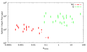
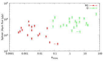
Figure 2.— Core dominance versus infrared fluxes (top: 3.6 $\mu$m; bottom: 24 $\mu$m), inspired by what was presented in Haas et al. (2008). Radio galaxies are shown with red circles, quasars with green triangles.

Figure 3.— Plot of the near (3.6 $\mu$m) and mid (24 $\mu$m) infrared fluxes. The color code is the same as in Fig. 2.

Fig. 2 shows the radio core dominance parameter versus NIR (top) and MIR (bottom) fluxes. We see that the 3.6 $\mu$m RG fluxes are, on average, a factor 6.3 lower than the quasar fluxes (median: 6.8), which is in good agreement with the quasar/radio-galaxy flux ratios (2.5 – 7.5) found by Hönig et al. (2011) at 3.5 $\mu$m. The same conclusions apply for the 24 $\mu$m fluxes against R_5GHz, where the MIR emission is found to be more isotropic. Due to the dispersion of data points, the flux ratio is more complicated to estimate but the averaged value is 3.3 (median: 3.4).

The flux ratio between NIR and MIR emission is shown in Fig. 3. The radio-galaxies are below the quasars on average, by a factor $\sim$ 1.35. There is a fairly low dispersion among the quasars as their IR SEDs are generic; in the case of radio-galaxies the distribution is less tight as RG show less uniformity than quasars (Hönig et al., 2011). For a a given 24 $\mu$m flux, the 3.6 $\mu$m flux is much lower for the radio galaxies, as expected from the obscuration paradigm. Finally, it seems that we are also detecting an inclination-dependence of the NIR/MIR flux ratio within each class in the expected sense.

Our conclusions that the $z\geq$ 1 3CRR radio galaxies have several times weaker NIR and MIR emission compared with the matched quasars, and more varied SEDs, are not new. They were stated explicitly by Haas et al. (2008), Podigachoski et al. (2015), and references therein; Hönig et al. (2011) shows quotient spectra for radio galaxies over quasars. For lower redshift 3CR objects, Ogle et al. (2006) reported these effects, with references to much earlier work . The novel aspect here is again to exploit the near perfect separation of the classes by IR colors to constrain deviations from the simplest unified model.

II.3. … and optical polarization

The infrared fluxes have shown excellent agreement with the expectation from the unified model and strongly corroborate our finding that there is an almost perfect separation between the two optical classes of radio-loud AGN based on R_5GHz. Nevertheless, we decided to do a third check using near-ultraviolet, optical and near-IR continuum polarization measurements from the literature. The unified model again makes strong predictions about the degree and orientation of AGN polarization and we expect a clear dichotomy between type-1 and type-2 AGN. Our sample is too small to demonstrate the predicted relationships by itself, but we can check for consistency.

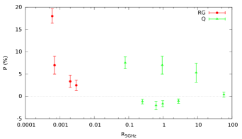
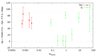
Figure 4.— Optical continuum polarization versus core dominance. Top: linear polarization degree $P$; bottom: difference ($\Delta\psi$) between the radio position angle PA and the optical polarization position angle $PPA$. We use the following convention: $P$ is plotted as negative when the $\vec{E}$-vector of the continuum radiation aligns with the projected axis of the (small-scale) radio structures ($PPA$ = 90^∘), and $P$ is positive for perpendicular polarization ($PPA$ = 0^∘). The horizontal lines show the minimum and maximum realizable value for the position angle difference. The color code is the same as in Fig. 2.

Tab. 1 lists the only 13 polarimetric data reported for the 3CRR objects in our sample. These AGN have been observed in U, B, V and/or R polarization filters, and were corrected for the small polarizations of the instrument and the Galactic interstellar medium. The polarization degree $P$ and the difference $\Delta\psi$ between the radio position angle PA and the optical polarization position angle $PPA$ are presented in Fig. 4 top and bottom, respectively. $P$ seems similar between RG and quasars, but radio galaxies are generally substantially diluted by starlight, while that of quasars is not (Cimatti et al., 1997), which is part of the reason why the polarization degree of the two groups seems similar. However, there is a net difference between type-1 and type-2 AGN: RG only show a polarization position angle approximately perpendicular to the projected axis of the radio structures ($\Delta\psi$ = 90^∘) while quasars are characterized by a blend of perpendicular and parallel polarization angles. The exact same dichotomy appears in radio-quiet AGN (Antonucci, 1993) and radio-loud AGN at lower redshifts (Antonucci, 1984), where type-2s have perpendicular $PPA$ only. The presence of perpendicular $PPA$ indicates that photons dominantly experience scattering in polar directions, while a parallel $PPA$ is the signature of equatorial scattering. Polar scattering dominated quasars tend to have higher degrees of polarization (up to a couple of percents) than equatorial scattering quasars, as already observed for their radio-quiet analogues (Smith et al., 2002). A large part of the higher polarization in well-studied type-2 AGN results from the fact that the direct light from the quasar is blocked; otherwise it would dilute the observed polarization, often very strongly. However, the relatively high polarization of the polar-scattered quasars indicates that our inclination-dependent view of the scattering medium also plays a role. Finally, we note that the incidence of high parallel polarization in the quasars is much higher than in other well-studied samples (Stockman et al., 1979), although it’s not clear why this should be the case.

III. A semi-empirical function of core dominance as a function of inclination

Since we are very confident that core dominance is a good qualitative inclination indicator, and that the sources are distributed uniformly in solid angle (Copernican Principle), we can make a quantitative semi-empirical function for the average inclination $i$ as a function of core dominance. It should be of interest to both observers and theorists (Blandford & Königl, 1979). To do so, we equally distributed the sources in solid angle and numerically fitted the relation using a polynomial regression. We obtained the following semi-empirical relation between core dominance and AGN inclination:

$$log({\rm R}_{\rm 5GHz})={\rm a}+{\rm b}i+{\rm c}i^{2}+{\rm d}i^{3}+{\rm e}i^{4}+{\rm f}i^{5},$$

or, if numerically inverted :

$$i={\rm g}+{\rm h}(LR)+{\rm j}(LR)^{2}+{\rm k}(LR)^{3}+{\rm l}(LR)^{4}+{\rm m}(LR)^{5},$$

with LR = $\log({\rm R}_{\rm 5GHz})$. The first formula, essentially the polar diagram for core emission, should be more useful to theorists, while the second version is directly useful to observers wishing to estimate the inclination for a given system.

Table 2Parametrization of the fits and goodness measures

Parameter for R(i)	Value
a	2.916 $\pm$ 0.124
b	-0.225 $\pm$ 0.027
c	0.009 $\pm$ 0.002
d	-1.799$\times$10-4 $\pm$ 4.987$\times$10-5
e	1.347$\times$10-6 $\pm$ 5.941$\times$10-7
f	-2.927$\times$10-9 $\pm$ 2.557$\times$10-9
Goodness measures	Value
$\cal{R}$2	0.9986
a$\cal{R}$2	0.9978
SE (in units of R5GHz)	0.0816
Parameter for i(R)	Value
g	41.799 $\pm$ 1.190
h	-20.002 $\pm$ 1.429
j	-4.603 $\pm$ 1.347
k	0.706 $\pm$ 0.608
l	0.663 $\pm$ 0.226
m	0.062 $\pm$ 0.075
Goodness measures	Value
$\cal{R}$2	0.9931
a$\cal{R}$2	0.9905
SE (in units of $i$)	2.7244

The parameters “a” and “g” are constants that represent the equivalent emission of an isotropic component. Values for $a$, $b$, $c$, $d$, $e$, $f$, $g$, $h$, $j$, $k$, $l$, and $m$, are given in Tab. 2, together with the goodness measures of the fitting function to the distribution of the sources in solid angle. The typical uncertainty in $i$ can be no more than about $\pm$ 10^∘; otherwise simulations show that the RG and quasars would overlap substantially. The number distribution resulting from this analytical formula is shown in Fig. 5 (top). Our new function properly reproduces the observed increase of quasar number at large R_5GHz and predicts that the distribution should be almost uniform in $i$ at large inclinations. Note that our formula must not be used in highly core-dominant objects, since the distribution is not sampled well at small inclinations.

Although we don’t have many sources, we can estimate the averaged half-opening angle of the circumnuclear region by estimating the ratios of type-1 to type-2 objects in out complete sample, which is 0.574, corresponding to a critical inclination of 55^∘ (60^∘ if excluding the two peculiar quasars mentioned in Sect. II.1). This result agrees with the values found by previous authors, including Barthel (1989), Arshakian (2005), Sazonov et al. (2015) and many others, who looked at high-luminosity radio-loud AGN and estimated that the half-opening angle of the equatorial region is $\sim$ 45^∘ – 60^∘. In the future we may enlarge our sample, or explore other parameter space using the same methods.

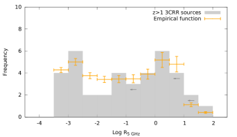
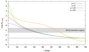
Figure 5.— Comparing our semi-empirical function (solid orange line) with the 3CRR sample (top figure) and the relativistic beaming model (bottom) presented in Orr & Browne (1982) for different $\gamma$ factors.

We plotted R_5GHz as a function of $i$ in Fig. 5 (bottom), together with the analytical formula from Orr & Browne (1982), where it is assumed that jets are co-linear (zero opening angle) and moving with a single bulk velocity, so that R_5GHz($i$) is just determined by special relativity. When compared with this naive model, our semi-empirical formula shows much stronger than predicted core fluxes at intermediate angles, so that the polar diagram is not as sharply peaked at $i$ = 0 as in the toy model. Taken at face value, the bulge in the polar emission diagram at $i\sim$ 40^∘ is consistent with the popular spine-and-sheath model (Sol et al., 1989), where there is a slow jacket to a fast very narrow jet. The slower sheet (layer) is only modestly beamed and substantial broadening of the effective beaming cone is required. This indicates a range of bulk speeds among objects or within individual jets, a range of direction of synchrotron-emitting plasma elements, optical depth effects, or other deviations from the single-zone jet (Blandford & Königl, 1979). However, our sample is small and better statistics are needed to evaluate the statistical significance of the bulge and, more generally, of the R(i) formula.

IV. Summary, discussion, and conclusions

We have demonstrated that the radio core dominance parameter R_5GHz separates the radio-galaxies and quasars almost perfectly in the $z\geq$ 1 3CRR sample. In other words, the agreement of R_5GHz with optical type is not a coincidence, and probably both R_5GHz and optical type are reliable orientation indicators. Since the 3CRR catalog is a complete sample, it must fill the solid angle uniformly, except for small number statistics, just from the Copernican Principle. Therefore we were able to derive an empirical core dominance formula, where R_5GHz is a function of inclination $i$. The essentially perfect separation of the optical types by radio core dominance and infrared (and X-ray columns) is most simply interpreted as meaning that there is only a small dispersion of opening angle, and no holes in the circumnuclear region which would let us see a type-1 AGN at high inclination (contrary to the hypothesis of Obied et al. 2016).

At lower luminosities, such predictions are less clear as the sample gets less clean. It is possible to extend the catalog to lower redshifts but it would be necessary to exclude nonthermal RG. Weakly-accreting radio-galaxies mostly radiate through kinetic energy in the form of synchrotron jets and lack highly ionized line emission and strong IR reprocessing bumps, which indicates that they lack energetically significant hidden quasars (Antonucci 2012 and references therein). It is then essential to remove them to have a correct sample.

At higher redshifts another problem may arise due to the fact that the ratio of lobe emission to jet power is sensitive to environment (Barthel & Arnaud, 1996). The density of the intergalactic medium (IGM) scales with redshift as (1 + $z$)³ (Macquart & Koay, 2013). For a $z$ = 5 quasar, the IGM density is 27 times higher than compared to a $z$ = 1 quasar, and these should strongly affect the morphology, lobe flux ratios, and lobe distance.

References

- Antonucci (1984) Antonucci, R. R. J. 1984, ApJ, 278, 499
- Antonucci (1993) Antonucci, R. 1993, ARA&A, 31, 473
- Antonucci (2012) Antonucci, R. 2012, Astronomical and Astrophysical Transactions, 27, 557
- Arshakian (2005) Arshakian, T. G. 2005, A&A, 436, 817
- Barthel (1989) Barthel, P. D. 1989, ApJ, 336, 606
- Barthel et al. (2000) Barthel, P. D., Vestergaard, M., & Lonsdale, C. J. 2000, A&A, 354, 7
- Barthel & Arnaud (1996) Barthel, P. D., & Arnaud, K. A. 1996, MNRAS, 283, L45
- Blandford & Königl (1979) Blandford, R. D., & Königl, A. 1979, ApJ, 232, 34
- Boksenberg et al. (1976) Boksenberg, A., Carswell, R. F., & Oke, J. B. 1976, ApJL, 206, L121
- Brotherton et al. (1998) Brotherton, M. S., Wills, B. J., Dey, A., van Breugel, W., & Antonucci, R. 1998, ApJ, 501, 110
- Cimatti et al. (1997) Cimatti, A., Dey, A., Breugel, W. v., Hurt, T., & Antonucci, R. 1997, ApJ, 476, 677
- Dey (1999) Dey, A. 1999, The Most Distant Radio Galaxies, 19, Proceedings of the colloquium, Amsterdam, 15-17 October 1997, Royal Netherlands Academy of Arts and Sciences. Edited by H. J. A. Röttgering, P. N. Best, and M. D. Lehnert
- Drouart et al. (2012) Drouart, G., De Breuck, C., Vernet, J., et al. 2012, A&A, 548, A45
- Elvis et al. (1994) Elvis, M., Wilkes, B. J., McDowell, J. C., et al. 1994, ApJS, 95, 1
- Fan et al. (2011) Fan, J.-H., Yang, J.-H., Pan, J., & Hua, T.-X. 2011, Research in Astronomy and Astrophysics, 11, 1413
- Fanti et al. (1995) Fanti, C., Fanti, R., Dallacasa, D., et al. 1995, A&A, 302, 317
- Fanti et al. (2002) Fanti, C., Fanti, R., Dallacasa, D., et al. 2002, A&A, 396, 801
- Gelderman & Whittle (1994) Gelderman, R., & Whittle, M. 1994, ApJS, 91, 491
- Haas et al. (2008) Haas, M., Willner, S. P., Heymann, F., et al. 2008, ApJ, 688, 122-127
- Heckman et al. (1994) Heckman, T. M., O’Dea, C. P., Baum, S. A., & Laurikainen, E. 1994, ApJ, 428, 65
- Hes et al. (1995) Hes, R., Barthel, P. D., & Hoekstra, H. 1995, A&A, 303, 8
- Hoekstra et al. (1997) Hoekstra, H., Barthel, P. D., & Hes, R. 1997, A&A, 319, 757
- Hough et al. (1999) Hough, D. H., Zensus, J. A., Vermeulen, R. C., et al. 1999, ApJ, 511, 84
- Hough et al. (2002) Hough, D. H., Vermeulen, R. C., Readhead, A. C. S., et al. 2002, AJ, 123, 1258
- Hönig et al. (2011) Hönig, S. F., Leipski, C., Antonucci, R., & Haas, M. 2011, ApJ, 736, 26
- Laing et al. (1983) Laing, R. A., Riley, J. M., & Longair, M. S. 1983, MNRAS, 204, 151
- Lawrence (1991) Lawrence, A. 1991, MNRAS, 252, 586
- Leipski et al. (2010) Leipski, C., Haas, M., Willner, S. P., et al. 2010, ApJ, 717, 766
- Ludke et al. (1998) Ludke, E., Garrington, S. T., Spencer, R. E., et al. 1998, MNRAS, 299, 467
- Macquart & Koay (2013) Macquart, J.-P., & Koay, J. Y. 2013, ApJ, 776, 125
- Marin (2014) Marin, F. 2014, MNRAS, 441, 551
- Marin (2016) Marin, F. 2016, MNRAS, in print
- Obied et al. (2016) Obied, G., Zakamska, N. L., Wylezalek, D., & Liu, G. 2016, MNRAS, 456, 2861
- Ogle et al. (2006) Ogle, P., Whysong, D., & Antonucci, R. 2006, ApJ, 647, 161
- Orr & Browne (1982) Orr, M. J. L., & Browne, I. W. A. 1982, MNRAS, 200, 1067
- Podigachoski et al. (2015) Podigachoski, P., Barthel, P., Haas, M., Leipski, C., & Wilkes, B. 2015, ApJL, 806, L11
- Podigachoski et al. (2016) Podigachoski, P., Barthel, P. D., Peletier, R. F., & Steendam, S. 2016, A&A, 585, A142
- Roger et al. (1973) Roger, R. S., Costain, C. H., & Bridle, A. H. 1973, AJ, 78, 1030
- Rawlings & Saunders (1991) Rawlings, S., & Saunders, R. 1991, Nature, 349, 138
- Sanders et al. (1989) Sanders, D. B., Phinney, E. S., Neugebauer, G., Soifer, B. T., & Matthews, K. 1989, ApJ, 347, 29
- Sazonov et al. (2015) Sazonov, S., Churazov, E., & Krivonos, R. 2015, MNRAS, 454, 1202
- Scarrott et al. (1990) Scarrott, S. M., Rolph, C. D., & Tadhunter, C. N. 1990, MNRAS, 243, 5P
- Scheuer & Readhead (1979) Scheuer, P. A. G., & Readhead, A. C. S. 1979, Nature, 277, 182
- Smith et al. (2002) Smith, J. E., Young, S., Robinson, A., et al. 2002, MNRAS, 335, 773
- Sol et al. (1989) Sol, H., Pelletier, G., & Asseo, E. 1989, MNRAS, 237, 411
- Stockman et al. (1979) Stockman, H. S., Angel, J. R. P., & Miley, G. K. 1979, ApJL, 227, L55
- Tadhunter (2005) Tadhunter, C. 2005, Astronomical Polarimetry: Current Status and Future Directions, 343, 457
- Urry & Padovani (1995) Urry, C. M., & Padovani, P. 1995, PASP, 107, 803
- Wilkes et al. (1999) Wilkes, B. J., Hooper, E. J., McLeod, K. K., et al. 1999, The Universe as Seen by ISO, 427, 845. Eds. P. Cox & M. F. Kessler. ESA-SP 427
- Wilkes et al. (2013) Wilkes, B. J., Kuraszkiewicz, J., Haas, M., et al. 2013, ApJ, 773, 15
- Willott et al. (2000) Willott, C. J., Rawlings, S., & Jarvis, M. J. 2000, MNRAS, 313, 237
- Wills & Brotherton (1995) Wills, B. J., & Brotherton, M. S. 1995, ApJL, 448, L81
- Zirbel & Baum (1995) Zirbel, E. L., & Baum, S. A. 1995, ApJ, 448, 521