Explanation of $B\to K^{(*)}\ell^{+}\ell^{-}$ and muon $g-2$,
and implications at the LHC

Abstract

More than $3\sigma$ deviations from the standard model are observed in the angular observable $P^{\prime}_{5}$ of $B\to K^{*}\mu^{+}\mu^{-}$ and muon $g-2$. To resolve these anomalies, we extend the standard model by adding two leptoquarks. It is found that the signal strength of the diphoton Higgs decay can exhibit a significant deviation from unity and is within the data errors. Although $\ell_{i}\to\ell_{j}\gamma$ puts severe bounds on some couplings, it is found that the excesses of $P^{\prime}_{5}$ and muon $g-2$ can still be explained and can be accommodated to the measurement of $B_{s}\to\mu^{+}\mu^{-}$ in this model. In addition, the leptoquark effects can also explain the LHCb measurement of $R_{K}=BR(B^{+}\to K^{+}\mu^{+}\mu^{-})/BR(B^{+}\to K^{+}e^{+}e^{-})=0.745^{+0.090}_{-0.074}\pm 0.036$, which shows a $2.6\sigma$ deviation from the standard model prediction.

I Introduction

The standard model (SM) has been tested at an unprecedented level of precision through various experiments. However, some excesses have not yet been completely resolved. The first case is the muon anomalous magnetic moment (muon $g-2$), where the discrepancy between experimental data and the SM prediction is currently $\Delta a_{\mu}=a^{\rm exp}_{\mu}-a^{\rm SM}_{\mu}=(28.8\pm 8.0)\times 10^{-10}$ PDG . The second case is the angular observable $P^{\prime}_{5}$ of $B\to K^{*}\mu^{+}\mu^{-}$ DescotesGenon:2012zf , where a $3.4\sigma$ deviation, resulting from the integrated luminosity of 3.0 fb^-1 at the LHCb Aaij:2015oid , recently confirmed an earlier result with $3.7\sigma$ deviations Aaij:2013qta . Moreover, the same measurement with $2.1\sigma$ deviations was reported by Belle Abdesselam:2016llu . Also, the other relevant $P_{i}$ observables are defined in Ref. Matias:2012xw . Various possible resolutions to this excess have been widely studied Descotes-Genon:2013wba ; Gauld:2013qja ; Datta:2013kja ; Hurth:2013ssa ; Descotes-Genon:2014uoa ; Altmannshofer:2014rta ; Crivellin:2015mga ; Sahoo:2015wya ; Straub:2015ica ; Crivellin:2015era ; Lee:2015qra ; Alonso:2015sja ; Sahoo:2015qha ; Sahoo:2015pzk ; Chiang:2016qov ; Belanger:2015nma ; Dorsner:2016wpm ; Becirevic:2015asa ; Descotes-Genon:2015uva ; Boucenna:2016wpr ; Hiller:2016kry . The third case is the ratio $R_{K}=BR(B^{+}\to K^{+}\mu^{+}\mu^{-})/BR(B^{+}\to K^{+}e^{+}e^{-})$, where $BR(B^{+}\to K^{+}\ell^{+}\ell^{-})$ is the branching ratio (BR) of the decay $B^{+}\to K^{+}\ell^{+}\ell^{-}$; and the LHCb measurement shows a $2.6\sigma$ deviation from the SM result Aaij:2014ora . In order to explain the deviation, various mechanisms have been proposed Crivellin:2015mga ; Hiller:2014yaa ; Hurth:2014vma ; Gripaios:2014tna ; Glashow:2014iga ; Sahoo:2015fla ; Bauer:2015knc ; Das:2016vkr ; Li:2016vvp ; Becirevic:2016yqi ; Sahoo:2016pet ; Bhattacharya:2016mcc ; Duraisamy:2016gsd .

In addition to the excesses mentioned above, the LHC with energetic $pp$ collisions can also be a good place to test the SM and provide possible excess signals. For instance, a hint of resonance with a mass of around 750 GeV in the diphoton invariant mass spectrum was indicated by the ATLAS Aaboud:2016tru and CMS Khachatryan:2016hje experiments. Due to the results, various proposals have been broadly proposed and studied Harigaya:2015ezk ; Backovic:2015fnp ; Angelescu:2015uiz ; Nakai:2015ptz ; Buttazzo:2015txu ; DiChiara:2015vdm ; Knapen:2015dap ; Pilaftsis:2015ycr ; Franceschini:2015kwy ; Ellis:2015oso ; Gupta:2015zzs ; Kobakhidze:2015ldh ; Falkowski:2015swt ; Benbrik:2015fyz ; Wang:2015kuj ; Dev:2015isx ; Allanach:2015ixl ; Wang:2015omi ; Chiang:2015tqz ; Huang:2015svl ; Ko:2016wce ; Nomura:2016seu ; Kanemura:2015bli ; Cheung:2015cug ; Nomura:2016fzs ; Ko:2016lai ; Belanger:2016ywb ; Dorsner:2016ypw ; Han:2016bvl ; Mambrini:2015wyu . Although it turns out that the resonance has not been confirmed by the updating data of ATLAS ATLAS:2016eeo and CMS CMS:2016crm and has been shown to be more like a statistical fluctuation, the search for the new exotic events in the LHC still continue and is an essential mission.

To resolve the excesses in a specific framework, we propose the extension of the SM by including leptoquarks (LQs), where the LQs are colored scalars that simultaneously couple to the leptons and quarks. Hence, the $b\to s\ell^{+}\ell^{-}$ decays can arise from the tree-level LQ-mediated Feynman diagrams when the muon $g-2$ is induced from LQ loops.

In addition to the decays $B\to K^{(*)}\ell^{+}\ell^{-}$, the effective interactions for $b\to s\ell^{+}\ell^{-}$ can also contribute to $B_{s}\to\mu^{+}\mu^{-}$, where the BR, measured by LHCb and CMS CMS:2014xfa , is given as:

$$\text{BR}(B_{s}\to\mu^{+}\mu^{-})^{\text{e}xp}=(2.8^{+0.7}_{-0.6})\times 10^{-9}\quad\quad\text{(LHCb-CMS)}\,.$$ (1)

We note that the dominant effective couplings for $b\to s\ell^{+}\ell^{-}$ processes are denoted by the Wilson coefficients $C_{9,10}$. Usually, both $C_{9}$ and $C_{10}$ are strongly correlated. Since this experimental result is consistent with the SM prediction of $\text{BR}(B_{s}\to\mu^{+}\mu^{-})^{\text{S}M}\approx 3.65\times 10^{-9}$ Bobeth:2013uxa , in order to accommodate the anomalies of $P^{\prime}_{5}$ and $R_{K}$ to the measurement of $B_{s}\to\mu^{+}\mu^{-}$, we introduce two LQs with different representations of $SU(2)_{L}$ into the model. Thus, the correlation between $C_{9}$ and $C_{10}$ is diminished. It is found that when the $C_{10}$ is constrained by $B_{s}\to\mu^{+}\mu^{-}$, the $C_{9}$ then can satisfy the requirements from the global analysis of $B\to K^{*}\mu^{+}\mu^{-}$, and can also explain the anomaly of $R_{K}$, and the muon $g-2$ can fit the current data.

The colored scalar LQs can couple to the SM Higgs in the scalar potential; thus, the LQ effects can influence the SM Higgs production and decays. The Higgs measurements have approached the precision level since the SM Higgs was discovered. Any sizable deviations from the SM predictions will indicate new physics. In this study, we analyze the LQ-loop contributions to the diphoton Higgs decay. It is worth mentioning that the introduced LQs can significantly enhance the production cross section of a heavy scalar boson if such heavy scalar is probed at the LHC in the future. The relevant studies on the heavy scalar production via LQ couplings can be found in Refs. DiIura:2016wbx ; Dey:2016sht ; Deppisch:2016qqd ; Hati:2016thk ; Chao:2015nac ; Murphy:2015kag ; Bauer:2015boy .

The paper is organized as follows. We introduce the model and discuss the relevant couplings in Sec. II. In Sec. III, we study the phenomena: the SM Higgs diphoton decay, LFV processes, Wilson coefficients of $C_{9,10}$ from LQ contributions for $b\to s\ell^{+}\ell^{-}$ decays, and the implication of $B_{s}\to\mu^{+}\mu^{-}$. The conclusion is given in Sec. IV.

II Couplings to the leptoquarks

In this section, we briefly introduce the model and relevant interactions with the LQs. To reconcile the measurements of $B_{s}\to\mu^{+}\mu^{-}$ and $B\to K^{*}\ell^{+}\ell^{-}$, we extend the SM by adding two different representations of LQ, which are $\Phi_{7/6}=(3,2)_{7/6}$ and $\Delta_{1/3}=(\bar{3},3)_{1/3}$ under $(SU(3)_{C},SU(2)_{L})_{U(1)_{Y}}$ SM gauge symmetry. The gauge-invariant Yukawa interactions of the SM fermions and LQs are written as:

$$L_{LQ}=k_{ij}\bar{Q}_{i}\Phi_{7/6}\ell_{Rj}+\tilde{k}_{ij}\bar{L}_{i}\tilde{\Phi}_{7/6}u_{Rj}+y_{ij}\bar{Q}_{i}^{c}i\sigma_{2}\Delta_{1/3}L_{j}+h.c.\,,$$ (2)

where the subscripts $i\,,j$ are the flavor indices; $L^{T}_{i}=(\nu_{i},\ell_{i}^{-})$ and $Q^{T}_{i}=(u_{i},d_{i})$ are the $SU(2)_{L}$ lepton and quark doublets, $\tilde{\Phi}_{7/6}=i\sigma_{2}\Phi^{*}_{7/6}$, and $(k_{ij},\tilde{k}_{ij},y_{ij})$ are the Yukawa couplings. Since we do not study the CP violating effects, hereafter, we take all new Yukawa couplings as real numbers. We use the representations of the LQs as:

$$\Phi_{7/6}=\begin{pmatrix}\phi^{5/3}\\ \phi^{2/3}\end{pmatrix}\,,\ \Delta_{1/3}=\begin{pmatrix}\delta^{1/3}/\sqrt{2}&\delta^{4/3}\\ \delta^{-2/3}&-\delta^{1/3}/\sqrt{2}\end{pmatrix}\,,$$ (3)

where the superscripts are the electric charges of the particles. The interactions in Eq. (2) are then expressed as:

$$L_{LQ}= k_{ij}\left[\bar{u}_{Li}\,\ell_{Rj}\phi^{5/3}+\bar{d}_{Li}\,\ell_{Rj}\phi^{2/3}\right]+\tilde{k}_{ij}\left[\bar{\ell}_{Li}\,u_{Rj}\phi^{-5/3}-\bar{\nu}_{Li}\,u_{Rj}\phi^{-2/3}\right]$$

$$+y_{ij}\left[\bar{u}^{c}_{Li}\,\nu_{Lj}\delta^{-2/3}-\frac{1}{\sqrt{2}}\bar{u}^{c}_{Li}\,\ell_{Lj}\delta^{1/3}-\frac{1}{\sqrt{2}}\bar{d}^{c}_{Li}\,\nu_{Lj}\delta^{1/3}-\bar{d}^{c}_{Li}\,\ell_{Lj}\delta^{4/3}\right]+h.c.$$ (4)

Since the LQs are colored scalar bosons, they can couple to the SM Higgs $H$ via the scalar potential. In order to get the Higgs couplings to the LQs, we write the gauge-invariant scalar potential as:

$$V =\mu^{2}H^{\dagger}H+\lambda(H^{\dagger}H)^{2}+M_{\Phi}^{2}\left(\Phi_{7/6}^{\dagger}\Phi_{7/6}\right)+M_{\Delta}^{2}Tr\left(\Delta_{1/3}^{\dagger}\Delta_{1/3}\right)+\lambda_{\Phi}\left(\Phi_{7/6}^{\dagger}\Phi_{7/6}\right)^{2}$$

$$+\lambda_{\Delta}\left[Tr\left(\Delta_{1/3}^{\dagger}\Delta_{1/3}\right)\right]^{2}+\lambda^{\prime}_{\Delta}Tr\left(\left[\Delta_{1/3}^{\dagger}\Delta_{1/3}\right]^{2}\right)+\lambda_{H\Phi}(H^{\dagger}H)\left(\Phi_{7/6}^{\dagger}\Phi_{7/6}\right)$$

$$+\lambda_{H\Delta}(H^{\dagger}H)Tr\left(\Delta_{1/3}^{\dagger}\Delta_{1/3}\right)+\lambda_{\Phi\Delta}\left(\Phi_{7/6}^{\dagger}\Phi_{7/6}\right)Tr\left(\Delta_{1/3}^{\dagger}\Delta_{1/3}\right)\,.$$ (5)

As usual, we adopt the representations of the Higgs doublet $H$ as:

$$H=\begin{pmatrix}G^{+}\\ \frac{1}{\sqrt{2}}(v+\phi+iG^{0})\end{pmatrix}\,,$$ (6)

where $G^{+}$ and $G^{0}$ are the Goldstone bosons; $\phi$ is the SM Higgs field, and $v$ is the vacuum expectation value (VEV) of $H$. It is known that the VEV of scalar field is dictated by the scalar potential.

III Phenomenological Analysis

Based on the introduced new interactions, in this section, we study the implications of the Higgs diphoton decay, $\ell_{i}\to\ell_{j}\gamma$, the muon $g-2$, $h\to\tau\mu$, $B\to K^{*}\ell^{+}\ell^{-}$, and $R_{K}$. Since each of these processes has its own unique characteristics, we discuss these phenomena one by one below.

III.1 Higgs diphoton decay

The Higgs measurement is usually described by the signal strength parameter, which is defined as the ratio of observation to the SM prediction and expressed as:

$$\mu^{f}_{i}=\frac{\sigma(pp\to h)}{\sigma(pp\to h)_{\rm SM}}\cdot\frac{\text{BR}(h\to f)}{\text{BR}(h\to f)_{\rm SM}}\equiv\mu_{i}\cdot\mu_{f}\,,$$ (7)

where $f$ stands for the possible channels, and $\mu_{i}(\mu_{f})$ denotes the signal strength of production (decay). Although vector-boson fusion (VBF) can also produce the SM Higgs, we only consider the gluon-gluon fusion (ggF) process because it is the most dominant. The diphoton Higgs decay approached the precision measurement since the 125 GeV Higgs was observed. Therefore, any significant deviation from the SM prediction (i.e., $\mu^{f}_{i}\neq 1$) can imply the new physical effects.

As stated earlier, the SM Higgs can couple to the LQs via the scalar potential. From Eq. (II), it can be seen that after spontaneous symmetry breaking (SSB), the quartic terms $H^{\dagger}H\Phi^{\dagger}_{7/6}\Phi_{7/6}$ and $H^{\dagger}HTr(\Delta^{\dagger}_{1/3}\Delta_{1/3})$ can lead to trilinear couplings of Higgs to LQs as:

$${\cal L} \supset\mu_{h\Phi}h\left(\phi^{-5/3}\phi^{5/3}+\phi^{-2/3}\phi^{2/3}\right)+\mu_{h\Delta}h\left(\delta^{-1/3}\delta^{1/3}+\delta^{-2/3}\delta^{2/3}+\delta^{-4/3}\delta^{4/3}\right)\,,$$ (8)

where $\mu_{h\Phi}=\lambda_{H\Phi}v$ and $\mu_{h\Delta}=\lambda_{H\Delta}v$. With the couplings in Eq. (8), the effective Lagrangian for $hgg$ by LQ-loop can be formulated as:

$$\Delta{\cal L}_{hgg}=\frac{\alpha_{s}}{8\pi}\left(\frac{\mu_{h\Phi}}{m_{\Phi}^{2}}A_{0}(\xi_{\Phi})+\frac{3\mu_{h\Delta}}{2m_{\Delta}^{2}}A_{0}(\xi_{\Delta})\right)hG^{a\mu\nu}G^{a}_{\mu\nu}\,,$$ (9)

where $\xi_{X}=4m_{X}^{2}/m_{h}^{2}$ and the loop function is given by:

$$A_{0}(x)=x(1-xf(x))$$ (10)

with $f(x)=\left[\sin^{-1}(1/\sqrt{x})\right]^{2}$ for $x>1$. Accordingly, the signal strength of the Higgs production and decay to diphoton can be respectively obtained as:

$$\mu_{i} =\left|1+\frac{v}{A_{1/2}(\xi_{t})}\sum_{X=\Phi,\Delta}\frac{n_{X}\mu_{hX}}{m^{2}_{X}}A_{0}(\xi_{X})\right|^{2}\,,$$

$$\mu_{\gamma\gamma} =\left|1+\frac{vN_{c}}{2}\frac{\sum_{X=\Phi,\Delta}Q^{2}_{X}A_{0}(\xi_{X})\mu_{hX}/m^{2}_{X}}{A_{1}(\xi_{W})+Q^{2}_{t}N_{c}A_{1/2}(\xi_{t})}\right|^{2},$$ (11)

where $n_{\Phi(\Delta)}=2(3)$, $N_{c}=3$ is the number of colors; $Q^{2}_{\Phi}=29/9$ and $Q^{2}_{\Delta}=21/9$, and the functions for vector-boson and fermion loops are given by

$$A_{1/2}(x) =-2[x+(1-x)f(x))]\,,$$

$$A_{1}(x) =2+3x+3(2x-x^{2})f(x)\,.$$ (12)

Since the effects of the doublet and triplet LQs are similar, for simplicity, we set $\mu_{h\Phi}=\mu_{h\Delta}=\mu_{LQ}$ and $m_{\Phi}=m_{\Delta}=m_{LQ}$. The $\mu^{\gamma\gamma}_{i}$ as a function of $m_{LQ}$ is presented in Fig. 1(a), and that of $\mu_{LQ}$ is shown in Fig. 1(b), where the curves in plot (a) are $\mu_{LQ}=0.1,0.5,1$ TeV, and those in plot (b) are $m_{LQ}=0.8,0.9,1.0$ TeV. For comparison, we also show the results of ATLAS Aad:2015gba and CMS CMS:2014ega with $1\sigma$ errors in the plots. From the plots, it can be clearly seen that with $\mu_{LQ}$ of ${\cal O}(100)$ GeV, the LQ contributions can significantly shift the $\mu^{\gamma\gamma}_{i}$ away from the SM prediction and that the results are consistent with the current data. On the contrary, the $\mu^{\gamma\gamma}_{i}$ approaches the SM result when $\mu_{LQ}$ is of the order of GeV.

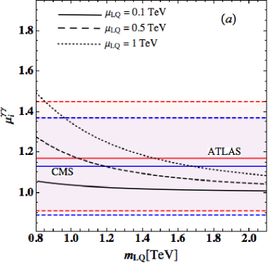
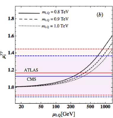
Figure 1: Diphoton signal strength parameter $\mu^{\gamma\gamma}_{i}$ as a function of (a) $m_{LQ}$ and (b) $\mu_{LQ}$, where the curves in plots (a) and (b) denote $\mu_{LQ}=(0.1,0.5,1)$ TeV and $m_{LQ}=(0.8,0.9,1.0)$ TeV, respectively.

III.2 Radiative and Higgs LFV processes, muon $g-2$, and $B\to K^{(*)}\ell^{+}\ell^{\prime-}$ decays

In the following analysis, we study the rare lepton-flavor violating processes, e.g. $\ell_{i}\to\ell_{j}\gamma$ and $h\to\bar{\tau}\mu+\bar{\mu}\tau$, muon $g-2$ $\Delta a_{\mu}$, and the FCNC process $B\to K^{*}\ell^{+}\ell^{-}$. We first discuss the radiative LFV processes for $\ell_{i}\to\ell_{j}\gamma$. With the couplings in Eq. (II), the LQ-loop induced decay amplitude for $\ell_{i}\to\ell_{j}\gamma$ can be written as:

$${\cal L}_{\ell_{i}\to\ell_{j}\gamma}=\frac{e}{2}\bar{\ell}_{j}\sigma_{\mu\nu}\left[(c_{L})_{ji}P_{L}+(c_{R})_{ji}P_{R}\right]\ell_{i}F^{\mu\nu}\,,$$ (13)

where the coefficient $(c_{R})_{ji}$ is expressed as:

$$(c_{R})_{ji} \approx\frac{m_{t}}{(4\pi)^{2}}(k^{\dagger})_{i3}\tilde{k}_{3j}\int d[X]\left(\frac{5}{\Delta(m_{t},m_{\Phi})}-\frac{2(1-x)}{\Delta(m_{\Phi},m_{t})}\right)\,,$$

$$\Delta(m_{1},m_{2}) =xm_{1}^{2}+(y+z)m_{2}^{2}\,,$$

$$\int[dX] =\int dxdydz\delta(1-x-y-z)\,,$$ (14)

$(c_{L})_{ji}$ can be obtained from $(c_{R})_{ji}$ by exchanging $k_{ab}$ and $\tilde{k}_{ab}$. In order to balance the chirality of the leptons, it is found that the contributions from $k^{\dagger}_{iq}k_{qj}$, $\tilde{k}^{\dagger}_{iq}\tilde{k}_{qj}$, $y^{\dagger}_{iq}k_{qj}$, and $y^{\dagger}_{iq}y_{qj}$ are suppressed by the lepton masses. Since the LQ $\phi^{5/3}$ can couple to left-handed and right-handed up-type quarks, the chirality flip by the mass insertion in the propagator of the up-type quark can lead to freeing of the lepton masses in the Feynman diagrams, which are associated with $k_{qi}$ and $\tilde{k}_{qi}$. In addition, the top-quark is much heavier than the $u$- and $c$-quarks; therefore, we only present the top-quark contribution in $(c_{R})_{ji}$. Straightforwardly, the BR for $\ell_{i}\to\ell_{j}\gamma$ can be expressed as:

$$\text{BR}(\ell_{i}\to\ell_{j}\gamma)=\frac{48\pi^{3}\alpha\eta_{i}}{G_{F}^{2}m_{\ell_{i}}^{2}}\left(\left|(c_{R})_{ji}\right|^{2}+\left|(c_{L})_{ji}\right|^{2}\right)\,,$$ (15)

where $\eta_{i}\simeq(1,1/5)$ for $i=(\mu,\tau)$ and the BRs for $\ell_{i}\to\ell_{j}\bar{\nu}_{j}\nu_{i}$ in the SM have been applied. The current experimental upper limits are shown in Table 1. According to Eq. (13), muon $g-2$ can be easily obtained by setting $j=i=\mu$ and found as:

$$\Delta a_{\mu}\simeq-\frac{m_{\mu}}{2}(c_{L}+c_{R})_{\mu\mu}.$$ (16)

Process	$(i,j)$	Experimental bounds ($90\%$ CL)
$\mu^{-}\to e^{-}\gamma$	$(2,1)$	$\text{BR}(\mu\to e\gamma)<5.7\times 10^{-13}$
$\tau^{-}\to e^{-}\gamma$	$(3,1)$	$\text{BR}(\tau\to e\gamma)<3.3\times 10^{-8}$
$\tau^{-}\to\mu^{-}\gamma$	$(3,2)$	$\text{BR}(\tau\to\mu\gamma)<4.4\times 10^{-8}$

Table 1: Current upper bounds on the BRs for the decays $\ell_{i}\to\ell_{j}\gamma$ Adam:2013mnn .

If the photon in $\ell_{i}\to\ell_{j}\gamma$ is replaced by the Higgs, similar Feynman diagrams can contribute to $h\to\bar{\ell}_{j}\ell_{i}+\bar{\ell}_{i}\ell_{j}\equiv\ell_{j}\ell_{i}$. Since the upper limit of $\text{BR}(\mu\to e\gamma)$ is of ${\cal O}(10^{-13})$ and can give strong constraints on the parameters $k^{\dagger}_{23}\tilde{k}_{31}$ and $\tilde{k}^{\dagger}_{23}k_{31}$, if we set $k_{31}$ and $\tilde{k}_{31}$ to be small, then it is apparent that $h\to e\mu$ and $h\to e\tau$ are much smaller than current upper limits. Hence, we just study the decay $h\to\mu\tau$. The one-loop induced effective couplings for $h\mu\tau$ are written as:

$$\mathcal{L}=h\bar{\mu}(C_{R}P_{R}+C_{L}P_{L})\tau+h.c.\,,$$ (17)

where $C_{L}$ is expressed as Baek:2015mea ; Baek:2016kud :

$$C_{L}= \frac{(k^{\dagger})_{23}\tilde{k}_{33}N_{c}m_{t}}{(4\pi)^{2}v}\left[A\left(\frac{m^{2}_{t}}{m^{2}_{\Phi}},\frac{m^{2}_{h}}{m^{2}_{\Phi}}\right)+B\left(\frac{m^{2}_{t}}{m^{2}_{\Phi}},\frac{m^{2}_{h}}{m^{2}_{\Phi}}\right)\right]$$

$$+\frac{N_{c}\mu_{h\Phi}}{(4\pi)^{2}}\sum_{i=1\text{-}3,q=u,d}\left[m_{\mu}(k^{\dagger})_{2i}k_{i3}G(m_{q_{i}},m_{\Phi})+m_{\tau}\tilde{k}^{\dagger}_{2i}\tilde{k}_{i3}\tilde{G}(m_{q_{i}},m_{\Phi})\right]$$

$$+\frac{N_{c}m_{\tau}\mu_{h\Delta}}{(4\pi)^{2}}\sum_{i=1\text{-}3,q=u,d}(y^{\dagger})_{2i}y_{i3}\tilde{G}(m_{q_{i}},m_{\Delta})\,,$$ (18)

$C_{R}$ can be obtained from $C_{L}$ by exchanging $k_{ab}$ and $\tilde{k}_{ab}$, and the loop functions are given by:

$$A(r_{t},r_{h})= -\frac{1}{2}-2\int[dX]\log\left[z+(1-z)r_{t}-xyr_{h}-i\epsilon\right]$$

$$+\int_{0}^{1}dx\log\left[x+(1-x)r_{t}-i\epsilon\right]\,,$$

$$B(r_{t},r_{h})= \int[dX]\frac{xyr_{h}-r_{t}}{z+(1-z)r_{t}-xyr_{h}}\,,$$

$$G(m_{1},m_{2})\approx \int[dX]\frac{z}{-xzm_{h}^{2}+xm_{1}^{2}+(y+z)m_{2}^{2}}\,,$$

$$\tilde{G}(m_{1},m_{2})\approx \int[dX]\frac{y}{-xzm_{h}^{2}+xm_{1}^{2}+(y+z)m_{2}^{2}}\,.$$ (19)

The $\epsilon$ in $A(r_{t},r_{h})$ denotes an infinitesimal positive value. It can be seen that the terms associated with $k^{\dagger}_{2i}k_{i3}$, $\tilde{k}^{\dagger}_{2i}k_{i3}$, and $y^{\dagger}_{2i}y_{i3}$ in Eq. (18) are proportional to the lepton masses. The situation is similar to the $(c_{R})_{ji}$ in the decays $\ell_{i}\to\ell_{j}\gamma$. Although $\mu_{hX}$ of TeV ($X=\Phi,\Delta)$ can enhance these effects, due to the effects of being related to $\mu_{hX}m_{\ell}/m^{2}_{X}$, their contributions are at least $10^{-2}$ smaller than those from $k^{\dagger}_{2i}\tilde{k}_{i3}$. Accordingly, the BR for $h\to\mu\tau$ is formulated as:

$$\text{BR}(h\to\mu\tau)\approx\frac{m_{h}}{16\pi\Gamma_{h}}(|C_{L}|^{2}+|C_{R}|^{2})\,,$$ (20)

where $\Gamma_{h}$ is the width of the Higgs. Due to $\text{BR}(h\to\mu\tau)$ being less than $1\%$, we use $\Gamma_{h}\approx\Gamma^{\rm SM}_{h}\approx 4.2$ MeV in our numerical estimations.

Next, we discuss the decays for $b\to s\ell^{+}\ell^{-}$. In order to include the effects of lepton non-unversality, we write the effective Hamiltonian as:

$${\cal H}=\frac{G_{F}\alpha V_{tb}V^{*}_{ts}}{\sqrt{2}\pi}\left[H_{1\mu}L^{\mu}+H_{2\mu}L^{5\mu}\right]\,,$$ (21)

where the leptonic currents are denoted by $L^{(5)}_{\mu}=\ell\gamma_{\mu}(\gamma_{5})\ell$; and the related hadronic currents are defined as:

$$H_{1\mu} =C^{\ell}_{9}\bar{s}\gamma_{\mu}P_{L}-\frac{2m_{b}}{q^{2}}C_{7}\bar{s}i\sigma_{\mu\nu}q^{\nu}P_{R}b\,,$$

$$H_{2\mu} =C^{\ell}_{10}\bar{s}\gamma_{\mu}P_{L}b\,.$$ (22)

Here, the Wilson coefficients are read as: $C^{\ell}_{9(10)}=C^{\rm SM}_{9(10)}+C^{\rm NP,\ell}_{9(10)}$ and $C_{7}=C^{\rm SM}_{7}$. The detailed angular distribution for $B\to(K\pi)_{K^{*}}\ell^{+}\ell^{-}$ can be found in Refs. DescotesGenon:2012zf ; Chen:2002bq ; Chen:2002zk ; Altmannshofer:2008dz ; Egede:2010zc . Following the notations in Ref. DescotesGenon:2012zf , the angular observable $P^{\prime}_{5}$ is defined by:

$$P^{\prime}_{5} =\frac{J_{5}}{\sqrt{-J_{2c}J_{2s}}}\,,\quad J_{5}=\sqrt{2}Re(A^{L}_{0}A^{L*}_{\perp})\,,$$

$$J_{2c} =-|A^{L}_{0}|^{2}\,,\quad J_{2s}=\frac{1}{4}\left(|A^{L}_{\parallel}|^{2}+|A^{L}_{\perp}|^{2}\right)\,,$$ (23)

where $A^{L}_{0,\parallel,\perp}$ are related to the $B\to K^{*}$ transition form factors and the Wilson coefficients of $C^{\ell}_{9,10}$ and $C_{7}$. Their explicit expressions can be found in Ref. DescotesGenon:2012zf . In this study, we do not directly investigate the angular analysis of $B\to K^{*}\ell^{+}\ell^{-}$; instead, we refer to the results, which were done by using the global analysis to get the best-fit value of $C^{NP}_{9}\approx-1.09$ for the new physics contributions Descotes-Genon:2015uva . Thus, we just derive the Wilson coefficients of $C^{\ell}_{9}$ and $C^{\ell}_{10}$ from the LQ contributions.

With the Yukawa couplings in Eq. (II), the effective Hamiltonian for $b\to s\ell^{+}\ell^{-}$ mediated by $\phi^{2/3}$ and $\delta^{4/3}$ can be respectively found as:

$$H_{\rm eff}^{1}=\frac{k_{b\ell}k_{s\ell}}{2m^{2}_{\Phi}}(\bar{s}\gamma^{\mu}P_{L}b)(\bar{\ell}\gamma_{\mu}P_{R}\ell)\,,$$

$$H_{\rm eff}^{2}=-\frac{y_{b\ell}y_{s\ell}}{2m^{2}_{\Delta}}(\bar{s}\gamma^{\mu}P_{L}b)(\bar{\ell}\gamma_{\mu}P_{L}\ell)\,.$$ (24)

We can decompose the Eq. (24) in terms of the effective operators $O_{9}$ and $O_{10}$, defined as $O_{9(10)}=\bar{s}\gamma_{\mu}P_{L}b\;\bar{\ell}\gamma^{\mu}(\gamma_{5})\ell$. The associated Wilson coefficients of $O_{9,10}$ from the LQs then are found as:

$$C^{LQ,\ell}_{9} =-\frac{1}{c_{\rm SM}}\left(\frac{k_{b\ell}k_{s\ell}}{4m^{2}_{\Phi}}-\frac{y_{b\ell}y_{s\ell}}{4m^{2}_{\Delta}}\right)\,,$$

$$C^{LQ,\ell}_{10} =\frac{1}{c_{\rm SM}}\left(\frac{k_{b\ell}k_{s\ell}}{4m^{2}_{\Phi}}+\frac{y_{b\ell}y_{s\ell}}{4m^{2}_{\Delta}}\right)\,,$$ (25)

where $c_{\rm SM}=V_{tb}V^{*}_{ts}\alpha G_{F}/(\sqrt{2}\pi)$ is a scale factor from the SM effective Hamiltonian. It is worth mentioning that the interaction $C^{LQ,\mu}_{10}O_{10}$ can contribute to $B_{s}\to\mu^{+}\mu^{-}$. Since the experimental data are consistent with the SM prediction, to consider the constraint from $B_{s}\to\mu^{+}\mu^{-}$, we adopt the expression for the BR as Hiller:2014yaa :

$$\frac{\text{BR}(B_{s}\to\mu^{+}\mu^{-})}{\text{BR}(B_{s}\to\mu^{+}\mu^{-})^{\text{S}M}}=\left|1-0.24C^{LQ,\mu}_{10}\right|^{2}.$$ (26)

With $1\sigma$ errors, the allowed range for $C^{LQ,\mu}_{10}$ is obtained as $C^{LQ,\mu}_{10}=(0.21,0.79)$. We use this result to constrain the free parameters. Since the $R_{K}$ is insensitive to the $B\to K$ transition form factors Hiller:2003js , in order to study the anomaly of $R_{K}$, we require that the allowed range of parameters has to satisfy Hiller:2014yaa :

$$0.7\leq Re[X^{e}-X^{\mu}]\leq 1.5\,,$$ (27)

where $X^{\ell}=C^{LQ,\ell}_{9}-C^{LQ,\ell}_{10}$, and the $R_{K}$ data with $1\sigma$ errors are used.

Since the parameters in the decays $\ell_{i}\to\ell_{j}\gamma$, $h\to\mu\tau$, $\Delta a_{\mu}$, and $B\to K^{(*)}\ell^{+}\ell^{-}$ are strongly correlated, in the following analysis, we take the current upper limits of $\text{BR}(\ell_{i}\to\ell_{j}\gamma)$ shown in Table 1 as the inputs and attempt to find the allowed parameter space, such that the excesses in $\Delta a_{\mu}$ and $B\to K^{(*)}\ell^{+}\ell^{-}$ can be satisfied, and the $\text{BR}(h\to\mu\tau)$ can be as large as possible.

From $(c_{R})_{ji}$ in Eq. (14), the dominant effects on the radiative LFV processes are from the $\phi^{5/3}$ and the top-quark loop; thus, there is no possible cancellation in any of the decay amplitudes. With the upper bound of $\text{BR}(\mu\to e\gamma)$, we see that $k^{\dagger}_{13}\tilde{k}_{32}$ and $\tilde{k}^{\dagger}_{13}k_{32}$ have to be very small. In order to explain the excesses of muon $g-2$ and $B\to K^{*}\mu^{+}\mu^{-}$, we set $k_{31}=\tilde{k}_{31}\approx 0$. As a result, $\text{BR}(h\to e\mu)$ is negligible in this model. The related parameters for $\tau\to(\mu,e)\gamma$ decays are $k_{31,32}\tilde{k}_{33}$ and $\tilde{k}_{31,32}k_{33}$, respectively. These parameters simultaneously influence $h\to(\mu,e)\tau$, muon $g-2$, and $b\to s\mu^{+}\mu^{-}$; therefore we have to analyze these processes together to get the allowed parameter space.

Since Eqs. (14), (18), and (25) involve many free parameters, in order to efficiently perform a numerical analysis, we set the ranges of relevant parameters as:

$$m_{LQ}\in[700\,,1500\,]\;\text{GeV},\quad\mu_{LQ}\in[1\,,100]\;\text{GeV}\,,\quad\{k_{22},\tilde{k}_{22},y_{22}\}\in[-0.1\,,0.1]\,,$$

$$\{k_{33},\tilde{k}_{33},y_{33}\}\in[-0.01,0.01]\,,\quad\{k_{23},\tilde{k}_{23},y_{23}\}\in[-0.1\,,0.1]\,,$$

$$k_{32}\in\text{sign}(k_{22})[0,0.5]\,,\quad\tilde{k}_{32}\in[-0.5\,,0.5]\,,\quad y_{32}\in-\text{sign}(y_{22})[0\,,0.5]\,.$$ (28)

In order to avoid the constraints from $\tau\to\ell\gamma$ ($\ell=e,\mu$) and get $|C^{LQ,\mu}_{9}|\sim 1$, we set ($k_{33}/k_{32},\tilde{k}_{33}/\tilde{k}_{32})\sim 0.1$ in Eq. (28). Additionally, the negative value of $C^{LQ,\mu}_{9}$ can be achieved when $k_{32}(y_{32})$ and $k_{22}(y_{22})$ are opposite in sign. As mentioned earlier, the Yukawa couplings in both decays $\tau\to\ell\gamma$ and $h\to\ell\tau$ are the same, we cannot remove the constraints from the radiative LFV processes in this model. The BRs for $h\to\ell\tau$ thus are of ${\cal}O(10^{-9})$ and much smaller than the current upper limits of ${\cal O}(10^{-4})$ Khachatryan:2015kon ; Aad:2015gha . One way to escape the constraint from $\tau\to\ell\gamma$ is to add a new LQ Baek:2015mea . Since we focus on the excesses of muon $g-2$ and $B\to K^{*}\mu^{+}\mu^{-}$, we leave the more complicated model for further study.

With the chosen ranges of parameters in Eq. (28), we first show the values for $C^{LQ,\mu}_{9}$ and $C^{LQ,\mu}_{10}$ in Fig. 2(a), where the bounds from $\tau\to\ell\gamma$ have been considered; the horizontal band is from the measurement of $B_{s}\to\mu^{+}\mu^{-}$; the vertical band is the range that can explain the excess of $B\to K^{*}\mu^{+}\mu^{-}$, and we used $10^{5}$ parameter sets and obtained $824$ allowed points that satisfy the constraints. It can be seen that the $C^{LQ,\mu}_{9}$ and $C^{LQ,\mu}_{10}$ from the contributions of doublet $\Phi_{7/6}$ and triplet $\Delta_{1/3}$ LQs can simultaneously satisfy the constraint of $B_{s}\to\mu^{+}\mu^{-}$ and explain the excess in $B\to K^{*}\mu^{+}\mu^{-}$.

From Eq. (16), it is known that muon $g-2$ is associated with the Yukawa couplings $k_{32}\tilde{k}_{32}$. Although only $k_{32}$ is related to $C^{LQ,\mu}_{9}$ and $C^{LQ,\mu}_{10}$, since the Yukawa couplings $k_{q\ell}$, $\tilde{k}_{q\ell}$, and $y_{q\ell}$ are taken to be the same order of magnitude, we present the correlations of $\Delta a_{\mu}$ and $C^{LQ,\mu}_{9}$ in Fig. 2(b), where only the allowed range of $C^{LQ,\mu}_{9}$ is shown, and the region between two dashed lines denotes the $\Delta a_{\mu}$ data with $1\sigma$ errors. By plot (b), it can be seen clearly that the excesses in $\Delta a_{\mu}$ and $B\to K^{*}\mu^{+}\mu^{-}$ can be simultaneously fitted in the model.

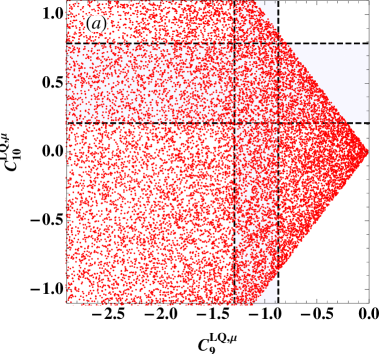
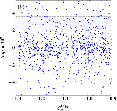
Figure 2: (a) The values of $C^{LQ,\mu}_{9}$ and $C^{LQ,\mu}_{10}$ using the ranges of parameters in Eq. (28), where the bound from the $\text{BR}(B_{s}\to\mu^{+}\mu^{-})$ and the allowed range of $C^{LQ,\mu}_{9}$ from global analysis for $B\to K^{*}\mu^{+}\mu^{-}$ are shown. (b) Correlation of $\Delta a_{\mu}$ and $C^{LQ,\mu}_{9}$, where we only show the values of $C^{LQ,\mu}_{9}$ that can fit the excess in $B\to K^{*}\mu^{+}\mu^{-}$, and the band bounded by two dashed lines denotes the $\Delta a_{\mu}$ data with $1\sigma$ errors PDG .

As discussed before, in order to avoid the constraint from $\mu\to e\gamma$, we set $k_{31}=\tilde{k}_{31}=0$ in our analysis; therefore, $C^{LQ,e}_{9(10)}$ for $B\to Ke^{+}e^{-}$ decay is only related to $y_{31}y_{21}$. Since $y_{31,21}$ are free parameters, for simplicity, we then take $|y_{31}|\sim|k_{31}|\sim 0$. As a result, $X^{e}=C^{LQ,e}_{9}-C^{LQ,e}_{10}\approx 0$. In order to see whether the obtained $C^{LQ,\mu}_{9}$ and $C^{LQ,\mu}_{10}$ can fit the $R_{K}$ data, we show the correlation between $X^{\mu}$ and $C^{LQ,\mu}_{9}$ in Fig. 3, where the band denotes the allowed range shown in Eq. (27). It can be seen that the excesses of $R_{K}$ and $P^{\prime}_{5}$ can be simultaneously explained when the measurement of $B_{s}\to\mu^{+}\mu^{-}$ is satisfied.

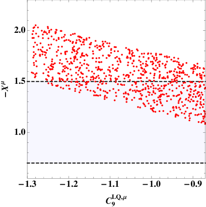
Figure 3: Correlation between $X^{\mu}=C^{LQ,\mu}_{9}-C^{LQ,\mu}_{10}$ and $C^{LQ,\mu}_{9}$, where the allowed range of $X^{\mu}$ is from the $R_{K}$ data with $1\sigma$ errors.

IV Conclusion

In order to resolve the excesses of muon $g-2$ and $B\to K^{(*)}\ell^{+}\ell^{-}$ decays, we investigate the extension of the SM by including leptoquarks, in which the particles are colored scalar bosons and can couple to quarks and leptons. In order to accommodate the measurement of $B_{s}\to\mu^{+}\mu^{-}$ and the excesses of $B\to K^{(*)}\mu^{+}\mu^{-}$, we study a model with one doublet and one triplet leptoquarks.

After SSB, the couplings of the SM Higgs the LQs are described by $\mu_{hX}=\lambda_{HX}v$. If $\mu_{hX}$ is of ${\cal O}(100)$ GeV, the signal strength parameter $\mu^{\gamma\gamma}_{i}$ can significantly deviate from the SM prediction and is still consistent with the current Higgs measurements.

In this study, lepton-flavor violating processes $\ell_{i}\to\ell_{j}\gamma$ give strict constraints on the Yukawa couplings $k_{31,33}$ and $\tilde{k}_{31,33}$. As a result, the branching ratios for the lepton-flavor violating Higgs decays $h\to\ell_{i}\ell_{j}$ are less than ${\cal O}(10^{-8}$). Nevertheless, the sizable couplings $k_{32,22}$, $\tilde{k}_{32,22}$, and $y_{32,22}$ can still explain the excess of muon $g-2$ and provide the necessary values for the Wilson coefficient $C^{\ell}_{9}$, such that the excesses in $B\to K^{*}\mu^{+}\mu^{-}$ and $R_{K}$ can be resolved.

References

- (1) K.A. Olive et al. (Particle Data Group), Chin. Phys. C, 38, 090001 (2014).
- (2) S. Descotes-Genon, J. Matias, M. Ramon and J. Virto, JHEP 1301, 048 (2013) [arXiv:1207.2753 [hep-ph]].
- (3) R. Aaij et al. [LHCb Collaboration], JHEP 1602, 104 (2016) [arXiv:1512.04442 [hep-ex]].
- (4) R. Aaij et al. [LHCb Collaboration], Phys. Rev. Lett. 111, 191801 (2013) [arXiv:1308.1707 [hep-ex]].
- (5) A. Abdesselam et al. [Belle Collaboration], arXiv:1604.04042 [hep-ex].
- (6) J. Matias, F. Mescia, M. Ramon and J. Virto, JHEP 1204, 104 (2012) [arXiv:1202.4266 [hep-ph]].
- (7) S. Descotes-Genon, J. Matias and J. Virto, Phys. Rev. D 88, 074002 (2013) [arXiv:1307.5683 [hep-ph]].
- (8) R. Gauld, F. Goertz and U. Haisch, JHEP 1401, 069 (2014) [arXiv:1310.1082 [hep-ph]].
- (9) A. Datta, M. Duraisamy and D. Ghosh, Phys. Rev. D 89, no. 7, 071501 (2014) [arXiv:1310.1937 [hep-ph]].
- (10) T. Hurth and F. Mahmoudi, JHEP 1404, 097 (2014) [arXiv:1312.5267 [hep-ph]].
- (11) S. Descotes-Genon, L. Hofer, J. Matias and J. Virto, JHEP 1412, 125 (2014) [arXiv:1407.8526 [hep-ph]].
- (12) W. Altmannshofer and D. M. Straub, Eur. Phys. J. C 75, no. 8, 382 (2015) [arXiv:1411.3161 [hep-ph]].
- (13) S. Descotes-Genon, L. Hofer, J. Matias and J. Virto, JHEP 1606, 092 (2016) [arXiv:1510.04239 [hep-ph]].
- (14) A. Crivellin, G. D’Ambrosio and J. Heeck, Phys. Rev. Lett. 114, 151801 (2015) [arXiv:1501.00993 [hep-ph]].
- (15) S. Sahoo and R. Mohanta, Phys. Rev. D 91, no. 9, 094019 (2015) [arXiv:1501.05193 [hep-ph]].
- (16) A. Bharucha, D. M. Straub and R. Zwicky, arXiv:1503.05534 [hep-ph].
- (17) D. Becirevic, S. Fajfer and N. Kosnik, Phys. Rev. D 92, no. 1, 014016 (2015) [arXiv:1503.09024 [hep-ph]].
- (18) A. Crivellin, L. Hofer, J. Matias, U. Nierste, S. Pokorski and J. Rosiek, Phys. Rev. D 92, no. 5, 054013 (2015) [arXiv:1504.07928 [hep-ph]].
- (19) C. J. Lee and J. Tandean, JHEP 1508, 123 (2015) [arXiv:1505.04692 [hep-ph]].
- (20) R. Alonso, B. Grinstein and J. Martin Camalich, JHEP 1510, 184 (2015) [arXiv:1505.05164 [hep-ph]].
- (21) S. Sahoo and R. Mohanta, Phys. Rev. D 93, no. 3, 034018 (2016) [arXiv:1507.02070 [hep-ph]].
- (22) G. Belanger, C. Delaunay and S. Westhoff, Phys. Rev. D 92, 055021 (2015) [arXiv:1507.06660 [hep-ph]].
- (23) S. Sahoo and R. Mohanta, Phys. Rev. D 93, no. 11, 114001 (2016) [arXiv:1512.04657 [hep-ph]].
- (24) C. W. Chiang, X. G. He and G. Valencia, Phys. Rev. D 93, no. 7, 074003 (2016) [arXiv:1601.07328 [hep-ph]].
- (25) I. Dorsner, S. Fajfer, A. Greljo, J. F. Kamenik and N. Kosnik, Phys. Rept. 641, 1 (2016) [arXiv:1603.04993 [hep-ph]].
- (26) S. M. Boucenna, A. Celis, J. Fuentes-Martin, A. Vicente and J. Virto, Phys. Lett. B 760, 214 (2016) [arXiv:1604.03088 [hep-ph]].
- (27) G. Hiller, D. Loose and K. Schonwald, arXiv:1609.08895 [hep-ph].
- (28) R. Aaij et al. [LHCb Collaboration], Phys. Rev. Lett. 113, 151601 (2014) [arXiv:1406.6482 [hep-ex]].
- (29) G. Hiller and M. Schmaltz, Phys. Rev. D 90, 054014 (2014) [arXiv:1408.1627 [hep-ph]].
- (30) T. Hurth, F. Mahmoudi and S. Neshatpour, JHEP 1412, 053 (2014) [arXiv:1410.4545 [hep-ph]].
- (31) S. L. Glashow, D. Guadagnoli and K. Lane, Phys. Rev. Lett. 114, 091801 (2015) [arXiv:1411.0565 [hep-ph]].
- (32) B. Gripaios, M. Nardecchia and S. A. Renner, JHEP 1505, 006 (2015) [arXiv:1412.1791 [hep-ph]].
- (33) S. Sahoo and R. Mohanta, New J. Phys. 18, no. 1, 013032 (2016) [arXiv:1509.06248 [hep-ph]].
- (34) M. Bauer and M. Neubert, Phys. Rev. Lett. 116, no. 14, 141802 (2016) [arXiv:1511.01900 [hep-ph]].
- (35) D. Das, C. Hati, G. Kumar and N. Mahajan, Phys. Rev. D 94, no. 5, 055034 (2016) [arXiv:1605.06313 [hep-ph]].
- (36) X. Q. Li, Y. D. Yang and X. Zhang, JHEP 1608, 054 (2016) [arXiv:1605.09308 [hep-ph]].
- (37) D. Beirevi, S. Fajfer, N. Konik and O. Sumensari, arXiv:1608.08501 [hep-ph].
- (38) S. Sahoo, R. Mohanta and A. K. Giri, arXiv:1609.04367 [hep-ph].
- (39) B. Bhattacharya, A. Datta, J. P. Guevin, D. London and R. Watanabe, arXiv:1609.09078 [hep-ph].
- (40) M. Duraisamy, S. Sahoo and R. Mohanta, arXiv:1610.00902 [hep-ph].
- (41) M. Aaboud et al. [ATLAS Collaboration], arXiv:1606.03833 [hep-ex].
- (42) V. Khachatryan et al. [CMS Collaboration], arXiv:1606.04093 [hep-ex].
- (43) K. Harigaya and Y. Nomura, Phys. Lett. B 754, 151 (2016) [arXiv:1512.04850 [hep-ph]].
- (44) Y. Mambrini, G. Arcadi and A. Djouadi, Phys. Lett. B 755, 426 (2016) [arXiv:1512.04913 [hep-ph]].
- (45) M. Backovic, A. Mariotti and D. Redigolo, JHEP 1603, 157 (2016) [arXiv:1512.04917 [hep-ph]].
- (46) A. Angelescu, A. Djouadi and G. Moreau, Phys. Lett. B 756, 126 (2016) [arXiv:1512.04921 [hep-ph]].
- (47) Y. Nakai, R. Sato and K. Tobioka, Phys. Rev. Lett. 116, no. 15, 151802 (2016) [arXiv:1512.04924 [hep-ph]].
- (48) D. Buttazzo, A. Greljo and D. Marzocca, Eur. Phys. J. C 76, no. 3, 116 (2016) [arXiv:1512.04929 [hep-ph]].
- (49) S. Di Chiara, L. Marzola and M. Raidal, Phys. Rev. D 93, no. 9, 095018 (2016) [arXiv:1512.04939 [hep-ph]].
- (50) S. Knapen, T. Melia, M. Papucci and K. Zurek, Phys. Rev. D 93, no. 7, 075020 (2016) [arXiv:1512.04928 [hep-ph]].
- (51) A. Pilaftsis, Phys. Rev. D 93, no. 1, 015017 (2016) [arXiv:1512.04931 [hep-ph]].
- (52) R. Franceschini et al., JHEP 1603, 144 (2016) [arXiv:1512.04933 [hep-ph]].
- (53) J. Ellis, S. A. R. Ellis, J. Quevillon, V. Sanz and T. You, JHEP 1603, 176 (2016) [arXiv:1512.05327 [hep-ph]].
- (54) R. S. Gupta, S. Jager, Y. Kats, G. Perez and E. Stamou, arXiv:1512.05332 [hep-ph].
- (55) A. Kobakhidze, F. Wang, L. Wu, J. M. Yang and M. Zhang, Phys. Lett. B 757 (2016) 92 [arXiv:1512.05585 [hep-ph]].
- (56) A. Falkowski, O. Slone and T. Volansky, JHEP 1602, 152 (2016) [arXiv:1512.05777 [hep-ph]].
- (57) R. Benbrik, C. H. Chen and T. Nomura, Phys. Rev. D 93, no. 5, 055034 (2016) [arXiv:1512.06028 [hep-ph]].
- (58) F. Wang, L. Wu, J. M. Yang and M. Zhang, Phys. Lett. B 759 (2016) 191 [arXiv:1512.06715 [hep-ph]].
- (59) P. S. B. Dev and D. Teresi, arXiv:1512.07243 [hep-ph].
- (60) B. C. Allanach, P. S. B. Dev, S. A. Renner and K. Sakurai, Phys. Rev. D 93, no. 11, 115022 (2016) [arXiv:1512.07645 [hep-ph]].
- (61) K. Cheung, P. Ko, J. S. Lee, J. Park and P. Y. Tseng, arXiv:1512.07853 [hep-ph].
- (62) F. Wang, W. Wang, L. Wu, J. M. Yang and M. Zhang, arXiv:1512.08434 [hep-ph].
- (63) C. W. Chiang, M. Ibe and T. T. Yanagida, JHEP 1605, 084 (2016) [arXiv:1512.08895 [hep-ph]].
- (64) X. J. Huang, W. H. Zhang and Y. F. Zhou, Phys. Rev. D 93, 115006 (2016) [arXiv:1512.08992 [hep-ph]].
- (65) S. Kanemura, K. Nishiwaki, H. Okada, Y. Orikasa, S. C. Park and R. Watanabe, arXiv:1512.09048 [hep-ph].
- (66) T. Nomura and H. Okada, Phys. Lett. B 755, 306 (2016) [arXiv:1601.00386 [hep-ph]].
- (67) P. Ko, Y. Omura and C. Yu, JHEP 1604, 098 (2016) [arXiv:1601.00586 [hep-ph]].
- (68) P. Ko and T. Nomura, Phys. Lett. B 758, 205 (2016) [arXiv:1601.02490 [hep-ph]].
- (69) I. Dorsner, S. Fajfer and N. Kosnik, Phys. Rev. D 94, no. 1, 015009 (2016) [arXiv:1601.03267 [hep-ph]].
- (70) T. Nomura and H. Okada, arXiv:1601.04516 [hep-ph].
- (71) X. F. Han, L. Wang and J. M. Yang, Phys. Lett. B 757, 537 (2016) [arXiv:1601.04954 [hep-ph]].
- (72) G. Belanger and C. Delaunay, arXiv:1603.03333 [hep-ph].
- (73) The ATLAS collaboration [ATLAS Collaboration], ATLAS-CONF-2016-059.
- (74) CMS Collaboration [CMS Collaboration], CMS-PAS-EXO-16-027.
- (75) V. Khachatryan et al. [CMS and LHCb Collaborations], Nature 522, 68 (2015) [arXiv:1411.4413 [hep-ex]].
- (76) C. Bobeth, M. Gorbahn, T. Hermann, M. Misiak, E. Stamou and M. Steinhauser, Phys. Rev. Lett. 112, 101801 (2014) [arXiv:1311.0903 [hep-ph]].
- (77) M. Bauer and M. Neubert, Phys. Rev. D 93, no. 11, 115030 (2016) [arXiv:1512.06828 [hep-ph]].
- (78) C. W. Murphy, Phys. Lett. B 757, 192 (2016) [arXiv:1512.06976 [hep-ph]].
- (79) W. Chao, arXiv:1512.08484 [hep-ph].
- (80) C. Hati, Phys. Rev. D 93, no. 7, 075002 (2016) [arXiv:1601.02457 [hep-ph]].
- (81) F. F. Deppisch, S. Kulkarni, H. Pas and E. Schumacher, Phys. Rev. D 94, no. 1, 013003 (2016) [arXiv:1603.07672 [hep-ph]].
- (82) U. K. Dey, S. Mohanty and G. Tomar, arXiv:1606.07903 [hep-ph].
- (83) A. Di Iura, J. Herrero-Garcia and D. Meloni, arXiv:1606.08785 [hep-ph].
- (84) G. Aad et al. [ATLAS Collaboration], Eur. Phys. J. C 76 (2016) no.1, 6 [arXiv:1507.04548 [hep-ex]].
- (85) CMS Collaboration [CMS Collaboration], CMS-PAS-HIG-14-009.
- (86) J. Adam et al. [MEG Collaboration], Phys. Rev. Lett. 110, 201801 (2013) [arXiv:1303.0754 [hep-ex]].
- (87) S. Baek and K. Nishiwaki, Phys. Rev. D 93, no. 1, 015002 (2016) [arXiv:1509.07410 [hep-ph]].
- (88) S. Baek, T. Nomura and H. Okada, arXiv:1604.03738 [hep-ph].
- (89) C. H. Chen and C. Q. Geng, Nucl. Phys. B 636, 338 (2002) [hep-ph/0203003].
- (90) C. H. Chen and C. Q. Geng, Phys. Rev. D 66, 094018 (2002) [hep-ph/0209352].
- (91) W. Altmannshofer, P. Ball, A. Bharucha, A. J. Buras, D. M. Straub and M. Wick, JHEP 0901, 019 (2009) [arXiv:0811.1214 [hep-ph]].
- (92) U. Egede, T. Hurth, J. Matias, M. Ramon and W. Reece, JHEP 1010, 056 (2010) [arXiv:1005.0571 [hep-ph]].
- (93) G. Hiller and F. Kruger, Phys. Rev. D 69, 074020 (2004) [hep-ph/0310219].
- (94) V. Khachatryan et al. [CMS Collaboration], Phys. Lett. B 749, 337 (2015) [arXiv:1502.07400 [hep-ex]].
- (95) G. Aad et al. [ATLAS Collaboration], JHEP 1511, 211 (2015) [arXiv:1508.03372 [hep-ex]].