Accurate semilocal density functional for condensed matter physics and quantum chemistry

Abstract

Most density functionals have been developed by imposing the known exact constraints on the exchange-correlation energy, or by a fit to a set of properties of selected systems, or by both. However, accurate modeling of the conventional exchange hole presents a great challenge, due to the delocalization of the hole. Making use of the property that the hole can be made localized under a general coordinate transformation, here we derive an exchange hole from the density matrix expansion, while the correlation part is obtained by imposing the low-density limit constraint. From the hole, a semilocal exchange-correlation functional is calculated. Our comprehensive test shows that this functional can achieve remarkable accuracy for diverse properties of molecules, solids and solid surfaces, substantially improving upon the nonempirical functionals proposed in recent years. Accurate semilocal functionals based on their associated holes are physically appealing and practically useful for developing nonlocal functionals.

Kohn-Sham density functional theory (DFT) ks65 is a mainstream ground-state electronic structure theory, due to its high computational efficiency and useful accuracy. In this theory, everything is known, except for the exchange-correlation energy component, which has to be approximated as a functional of the electron density. Therefore, the central task of the theory is to develop consistently accurate exchange-correlation functional for wide-ranging problems. Many density functionals have been proposed PW86 ; B88 ; LYP88 ; BR89 ; B3PW91 ; PBE96 ; VSXC98 ; HCTH ; PBE0 ; HSE03 ; AE05 ; MO6L ; TPSS ; revTPSS ; PBEsol ; SCAN15 ; Kaup14 and some of them have been widely-used in electronic structure calculations of molecules and solids. Most of these functionals were constructed by imposing exact or nearly exact energy constraints PBE96 ; TPSS ; revTPSS ; PBEsol , or by a fit to a set of properties MO6L , or by their combination VSXC98 . Because exchange and correlation parts have different coordinate LP85 and spin OP79 scaling properties, they are usually approximated separately.

We begin with the exchange part. For simplicity, let us consider a spin-unpolarized system ($n_{\uparrow}=n_{\downarrow}$), for which the exchange energy is defined by

$$E_{x}=\frac{1}{2}\int d^{3}r\int d^{3}r^{\prime}\frac{n({\bf r})\rho_{x}({\bf r},{\bf r}^{\prime})}{|{\bf r}^{\prime}-{\bf r}|}.$$ (1)

(Atomic units $\hbar=e=m=1$ are used.) According to Eq. (1), the exchange energy is just the electrostatic interaction of each electron at ${\bf r}$ with the exchange hole at ${\bf r}^{\prime}$ surrounding the electron. The hole is conventionally defined as $\rho_{x}({\bf r},{\bf r}^{\prime})=-|\rho_{1}({\bf r},{\bf r}^{\prime})|^{2}/2n({\bf r})$, with $\rho_{1}({\bf r},{\bf r}^{\prime})=2\sum_{i=1}^{\mathrm{occup}}\psi_{i}^{*}({\bf r})\psi_{i}({\bf r}^{\prime})$ being the first-order reduced density matrix and $\psi_{i}$ being the occupied Kohn-Sham orbitals. We can see from Eq. (1) that the exchange energy is determined by the underlying exchange hole and the electron density $n({\bf r})$. The exchange hole is physically meaningful. For example, the system-averaged on-top ($|{\bf r}^{\prime}-{\bf r}|=0$) exchange hole TSP03 is proportional to the average electron density $\langle n\rangle$, while the latter is an experimental observable ADHyman78 . In addition, the hole can be also used to construct higher-level nonlocal density functionals such as range-separation functionals HSE03 ; Truhlar11 , which are particularly useful for the calculation of band gap and charge transfer. However, there is no simple procedure that can exactly extract the hole from a semilocal energy functional. In most cases, the hole has to be constructed with a reverse engineering approach PBY96 ; EP98 ; Henderson08 ; LAConstantin06 . This often introduces additional approximations. Therefore, it is highly desirable to approximate the exchange hole directly. The exchange energy functional can be easily generated from the associated hole.

The exchange hole can be approximated in several ways. For example, it can be constructed from the cutoff procedure PW86 ; PBE96 ; PBY96 . It can be also constructed from simple model systems BR89 . Here an exchange hole is derived from the density matrix expansion (DME) under a general coordinate transformation. Unlike the Taylor expansion B83 ; PEZB98 ; LAConstantin06 , the hole from the DME is not only correct for small separation (i.e., $|{\bf r}^{\prime}-{\bf r}|\approx 0$), but also properly converged in the large separation limit (see discussion below). In particular, it automatically recovers the exact uniform-gas limit. The convergence property enables us to obtain the exchange energy functional, without resort to any numerical cutoff procedure PW86 . Another advantage of the DME is that the exchange hole can be made localized with a general coordinate transformation TSP03 . This largely reduces the difficulty in the modeling of the highly nonlocal conventional hole.

The DME was originally introduced by Negele and Vautherin NV1 for the study of nuclear forces. Then it was generalized by Scuseria and co-workers VSXC98 ; KOS to calculate molecular properties, leading to the heavily-parametrized but accurate Voorhis-Scuseria functional VSXC98 , with 21 fitting parameters. This functional was re-parametrized by introducing more parameters by Zhao and Truhlar MO6L , leading to MO6L, one of the most popular semilocal functionals in quantum chemistry.

Here we introduce a novel technique in the DME. Our starting point is the general coordinate transformation KOS ; TSP03 $({\bf r},{\bf r}^{\prime})\rightarrow({\bf r}_{\lambda},{\bf u})$, where ${\bf r}_{\lambda}=\lambda{\bf r}+(1-\lambda){\bf r}^{\prime}$, ${\bf u}={\bf r}^{\prime}-{\bf r}$, with $\lambda$ being a real number between $1/2$ and 1. Since the Jacobian of the coordinate transformation is 1, Eq. (1) can be rewritten as TSP03

$$E_{x}=\frac{1}{2}\int d^{3}r_{\lambda}n({\bf r}_{\lambda})\int d^{3}u\frac{\rho_{x}^{t}({\bf r}_{\lambda},{\bf u})}{u},$$ (2)

where $\rho_{x}^{t}({\bf r}_{\lambda},{\bf u})$ is the transformed exchange hole defined by $\rho_{x}^{t}({\bf r}_{\lambda},{\bf u})=|\rho_{1}^{t}({\bf r}_{\lambda}-(1-\lambda){\bf u},{\bf r}_{\lambda}+\lambda{\bf u})|^{2}/2n({\bf r}_{\lambda})$, with $\rho_{1}^{t}({\bf r}_{\lambda}-(1-\lambda){\bf u},{\bf r}_{\lambda}+\lambda{\bf u})$ being the transformed density matrix. $\lambda=1$ corresponds to the conventional hole, while $\lambda=1/2$ corresponds to the hole in the center of mass.

Next, we expand the transformed Kohn-Sham single-particle density matrix about $u=0$:

$$\rho_{1}^{t}({\bf r},{\bf u})=e^{{\bf u}\cdot[-(1-\lambda)\mbox{\boldmath$\nabla$}_{1}+\lambda\mbox{\boldmath$\nabla$}_{2}]}\rho_{1}^{t}({\bf r},{\bf u})|_{u=0},$$ (3)

where $\mbox{\boldmath$\nabla$}_{1}$ and $\mbox{\boldmath$\nabla$}_{2}$ are the gradient operators acting on the first and second arguments of the transformed density matrix $\rho_{1}^{t}({\bf r},{\bf u})=\rho_{1}({\bf r}-(1-\lambda){\bf u},{\bf r}+\lambda{\bf u})$, respectively. For convenience, the subscript $\lambda$ has been dropped from now on. The Taylor expansion of the density matrix can yield the correct small-$u$ behaviour B83 ; PEZB98 ; LAConstantin06 , but the large-$u$ limit is divergent. Here we seek an expansion, which (i) recovers the exact uniform-gas limit, (ii) recovers the correct small-$u$ behaviour up to second order in $u^{2}$, and (iii) yields a converged large-$u$ limit. With these requirements, an exchange functional that respects the uniform-electron limit can be calculated from the transformed hole $\rho_{x}^{t}({\bf r},{\bf u})$ by performing integration over ${\bf u}$ in Eq. (2). To achieve this goal, we introduce a novel three-term Bessel-function and Legendre-polynomial expansion of a plane wave

$$e^{x{\rm cos}\theta y}=A+B+C,$$ (4)

where $A=\frac{1}{x}\sum_{l=0}^{\infty}(-1)^{l}(4l+3)j_{2l+1}(x)Q_{2l+1}(i{\rm cos}\theta y)$, $B=\frac{1}{x}\sum_{l=0}^{\infty}(-1)^{l}(4l+3)j_{2l+1}(x)y\frac{d}{dy}Q_{2l+1}(i{\rm cos}\theta y)$, $C=\frac{1}{x^{2}}\sum_{l=0}^{\infty}(-1)^{l}(4l+3)j_{2l+1}(x)\frac{1}{{\rm cos}\theta}\frac{d^{2}}{dy^{2}}Q_{2l+1}(i{\rm cos}\theta y)$, with $Q_{2l+1}(z)=P_{2l+1}(z)/z$. Eq. (4) can be derived with series resummation technique. (In previous works NV1 ; VSXC98 ; Tsuneda , a single-term Bessel-function and Legendre-polynomial expansion Arfken was used.) Substituting $x=ku$ and $y=[-(1-\lambda)\mbox{\boldmath$\nabla$}_{1}+\lambda\mbox{\boldmath$\nabla$}_{2}]/k$ into Eq. (4) and inserting Eq. (4) into Eq. (3) with the transformed density matrix $\rho_{1}^{t}({\bf r},{\bf u})$ lead to the DME expression

$$\rho_{1}^{t}({\bf r},{\bf u}) = 3n\frac{j_{1}(ku)}{ku}+\frac{35j_{3}(ku)}{2k^{3}u}G+\frac{105j_{3}(ku)}{2k^{3}u^{2}}H,~{}~{}$$ (5)

where $G=\{3{\rm cos}^{2}\theta[(\lambda^{2}-\lambda+1/2)\nabla^{2}n-2\tau]+3k^{2}n/5\}$, $H={\rm cos}\theta~{}(2\lambda-1)\nabla n$, with $\tau=\sum_{i}^{\rm occup}|\nabla\psi_{i}|^{2}$ being the kinetic energy density. In the derivation of Eq. (5), real orbitals are assumed. The first term on the right-hand side of Eq. (5) has the form of the density matrix of the uniform electron gas, while the second and third terms are $\lambda$-dependent inhomogeneous corrections. Clearly, the general coordinate transformation only affects inhomogeneous corrections, but not the extended uniform electron gas, because the latter is translationally invariant.

To evaluate the exchange energy, we only need the spherical average of the exchange hole over the direction of ${\bf u}$, which is determined by the spherical average of the square of the density matrix, $\langle|\rho_{1}^{t}({\bf r},{\bf u})|^{2}\rangle$ note1 . In Eq. (5), there is a parameter $k$, which has the dimension of the wave vector. $k=k_{F}$ is a natural choice for the uniform electron gas. For inhomogeneous systems, we set $k=fk_{F}$, where $f$ is a dimensionless parameter, depending on inhomogeneity VSXC98 . If we choose $\lambda=1$ (conventional exchange hole), $f$ may be fixed by imposing the sum rule GL76 on the model exchange hole, leading to

$$1/f^{3}+70y/(9f^{5})=1,$$ (6)

where $y=(2\lambda-1)^{2}p$ and $p=s^{2}=|\nabla n|^{2}/(2k_{F}n)^{2}$ is the square of the reduced density gradient. Here we treat $\lambda$ as a free parameter (which will be fixed later). It was shown JTao01 ; TSP03 that the exchange hole is not normalizable under the general coordinate transformation. However, as pointed out above, the general coordinate transformation only affects the properties of the hole for inhomogeneous systems. For slowly-varying densities, $1/f^{3}+70y/(9f^{5})\approx 1$, which yields $f\approx 1+70y/27$. As shown by Eq. (6), in the large-gradient limit, $f\rightarrow y^{1/5}$. This asymptotic behavior is consistent with Becke’s large-gradient dependence analysis B86 . Thus we assume that for any electron density,

$$f=[1+10(70y/27)+\beta y^{2}]^{1/10},$$ (7)

where $\beta$ is a parameter, which will be determined together with another parameter $\lambda$ later.

The exchange hole must be finite everywhere in space. However, the appearance of the Laplacian of the electron density in the DME of Eq. (5), which cannot be eliminated through the angle average of the square of the density matrix $\langle|\rho_{1}({\bf r},{\bf u})|^{2}\rangle$, can make the model exchange hole unphysically divergent at a nucleus. Therefore, we must eliminate the Laplacian in Eq. (5). This can be done with the second-order gradient expansion of the kinetic energy density, $\tau=\tau^{\rm unif}+|\nabla n|^{2}/(72n)+\nabla^{2}n/6$, where $\tau^{\rm unif}=(3/10)k_{F}^{2}n$ is the Thomas-Fermi kinetic energy density. This technique has been used in the development of semilocal DFT TPSS ; revTPSS and electron localization indicator TLZR05 . Replacing the Laplacian with $\nabla^{2}n=6[\tau-\tau^{\rm unif}-|\nabla n|^{2}/(72n)]$ in $\langle|\rho_{1}({\bf r},{\bf u})|^{2}\rangle$ [or Eq. (5)] yields the spherically-averaged exchange hole

$$\rho_{x}^{\rm t}=-\frac{9n}{2}\frac{j_{1}^{2}(ku)}{k^{2}u^{2}}-\frac{105j_{1}(ku)j_{3}(ku)}{k^{4}u^{2}}L-\frac{3675j_{3}^{2}(ku)}{8k^{6}u^{4}}M,$$ (8)

where $L=[3(\lambda^{2}-\lambda+1/2)(\tau-\tau^{\rm unif}-|\nabla n|^{2}/72n)-\tau+3k^{2}n/10]$, and $M=(2\lambda-1)^{2}|\nabla n|^{2}/n$. The exchange functional can be calculated from the hole by substituting Eq. (8) into Eq. (2) and using the Weber-Schafheitlin integral formula Luke62 . The result is

$$E_{x}[n]=\int d^{3}r~{}n\epsilon^{\rm unif}(n)F_{x}^{\rm DME}(p,\tau),$$ (9)

where $\epsilon^{\rm unif}(n)=-3k_{F}/4\pi$ is the exchange energy per electron of the uniform electron gas, and $F_{x}^{\rm DME}$ is the enhancement factor given by $F_{x}^{\rm DME}=1/f^{2}+7R/(9f^{4})$, with $R=1+595(2\lambda-1)^{2}p/54-[\tau-3(\lambda^{2}-\lambda+1/2)(\tau-\tau^{\rm unif}-|\nabla n|^{2}/72n)]/\tau^{\rm unif}$.

The two parameters $\lambda$ and $\beta$ can be determined by the following two conditions: (i) Recovery of the exchange energy of the H atom, and (ii) the least value that ensures $F_{x}^{\rm DME}$ to be a monotonically increasing and smooth function of the reduced density gradient $s$ in the iso-orbital region where $\tau=\tau_{W}=|\nabla n|^{2}/(8n)$. This yields $\lambda=0.6866$ and $\beta=79.873$. These two constraints were used in the construction of TPSS functional.

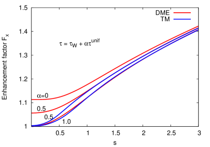
Figure 1: Enhancement factors $F_{x}^{\rm DME}$ of Eq. (9) (red) and $F_{x}^{\rm TM}$ of Eq. (11) (blue) in iso-orbital regions with $\alpha=0$ and orbital overlap regions with $\alpha=0.5,1.0$. $F_{x}^{\rm TM}=F_{x}^{\rm DME}$ at $\alpha=0$.

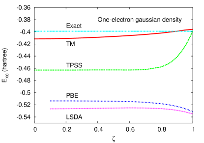
Figure 2: Exchange-correlation energy in the low-density limit for one-electron gaussian density with constant spin polarization TPSS ; JCP04 $n_{\uparrow}=[(1+\zeta)/(2\pi^{3/2})]e^{-r^{2}}$ and $n_{\downarrow}=[(1-\zeta)/(2\pi^{3/2})]e^{-r^{2}}$.

Table 1: Statistical errors of five nonempirical density functionals LSDA, PBE, TPSS, TMTPSS, and TM for 148 G2/97 atomization energies, 82 diatomic harmonic frequencies ($\omega_{e}$), 96 bond lengths ($r_{e}$), 10 hydrogen-bond (H-bond) dissociation energies and bond lengths, 16 lattice constants ($a_{0}$) and bulk moduli ($B_{0}$), 7 cohesive energies ($\epsilon_{\rm coh}$), and jellium surface exchange-correlation energies ($\sigma_{xc}$) for $r_{s}=2$-3. The data of the LSDA, PBE, and TPSS are taken from Refs. TPSS ; VNStaroverov04 ; JCP03 . The best values are in blue. ME = mean error and MAE = mean absolute error.

	AE6  G2 (kcal/mol)	$\omega_{e}$ (cm-1)	$r_{e}$ ($\AA$)	H-bond (kcal/mol)	H-bond length ($\AA$)	$~{}~{}~{}\sigma_{xc}$ (erg/cm2)	$a_{0}$ ($\AA$)	$B_{0}$ (GPa)	$\epsilon_{\rm coh}$ (eV)
	MAE  MAE	ME  MAE	ME  MAE	ME  MAE	ME  MAE	ME  MAE	ME  MAE	ME  MAE	ME  MAE
LSDA	77.3  83.5	$-11.8$  48.9	$0.001$  0.013	5.8  5.8	$-0.127$  0.147	$-78$  78	$-0.072$  0.072	12.6  13.2	0.68  0.68
PBE	15.5  18.3	$-31.7$  42.0	0.015  0.016	0.9  1.0	$-0.018$  0.043	$-133$  133	$-0.047$  0.050	$-4.2$  5.9	$-0.03$  0.12
TPSS	5.9  6.2	$-18.7$  30.4	0.014  0.014	0.3  0.6	$-0.006$  0.021	$-60$  60	$-0.034$  0.036	0.0  8.8	$-0.18$  0.18
TMTPSS	5.5  5.2	$-16.6$  29.0	0.013  0.013	$-0.5$  0.5	0.036  0.041	$-1$   1	0.005  0.019	4.9  7.3	$-0.13$  0.13
TM	5.1  6.5	$-16.6$  29.7	0.010  0.012	$-0.1$  0.3	0.014  0.017	35  35	$-0.003$  0.017	6.3  7.0	$-0.05$  0.08

The typical bulk valence electron density is slowly-varying. Recovery of the correct gradient expansion of the exchange energy is important for solids. It is also crucial for surface energy, because it involves the bulk solid contribution. However, the exchange energy functional and the underlying exchange hole from the DME are only exact in the uniform-gas limit, but not for slowly varying densities. To fix this problem, we propose the following interpolation formula between the compact density (where the DME is more suitable) and the delocalized slowly-varying density:

$$\rho_{x}({\bf r},{\bf u})=w\rho_{x}^{t}({\bf r},{\bf u})+(1-w)\rho_{x}^{\rm sc}({\bf r},{\bf u}),$$ (10)

with $w=[(\tau_{W}/\tau)^{2}+3(\tau_{W}/\tau)^{3}]/[1+(\tau_{W}/\tau)^{3}]^{2}$ being the weight between the compact density and the slowly varying correction (sc). (Other forms of $w$ are possible. This one provides a slightly more balanced interpolation between the compact density and the slowly varying density.) Near a bond center of molecules, $w\approx 0$ (except for one or two-electron systems, in which $w$ is identically 1 everywhere). In the core region and density tail, $w\approx 1$. In bulk solids, $w$ is small. $\rho_{x}^{\rm sc}({\bf r},{\bf u})$ can be obtained from the slowly varying gradient expansion of the exchange hole LAConstantin06 . This yields the final expression

$$F_{x}=wF_{x}^{\rm DME}+(1-w)F_{x}^{\rm sc},$$ (11)

where $F_{x}^{\rm sc}$ is the fourth-order gradient correction given by $F_{x}^{\rm sc}=\{1+10[(10/81+50p/729)p+146{\tilde{q}}^{2}/2025-(73{\tilde{q}}/405)[3\tau_{W}/(5\tau)](1-\tau_{W}/\tau)]\}^{1/10}$, with $\tilde{q}=(9/20)(\alpha-1)+2p/3$.

This completes the spin-unpolarized case. The hole and exchange energy functional can be easily generalized to any spin polarization, with the spin-scaling relation OP79 $\rho_{x}[n_{\uparrow},n_{\downarrow}]=(n_{\uparrow}/n)\rho_{x}[2n_{\uparrow}]+(n_{\downarrow}/n)\rho_{x}[2n_{\downarrow}]$. For convenience, we call it TM.

The density overlap region is an important region, where the magnitude of the first derivative of the density is small, but higher-order derivatives can be large. Therefore, it is a pseudo-slowly varying region. It includes intershell region in atoms, multiple-bond congestion region, and interstitial region in metals. This region can be modeled with $\tau=\tau_{W}+\alpha\tau_{0}$.

Figure 1 shows the variations of the enhancement factor $F_{x}^{\rm DME}$ [Eq. (9)] and its slowly-varying corrected version [Eq. (11)] from iso-orbital ($\alpha=0$) to overlap regions ($\alpha>0$) in the range $0\leq s\leq 3$. In the iso-orbital region, $F_{x}^{\rm TM}$ reduces to $F_{x}^{\rm DME}$, while in the overlap region, $F_{x}^{\rm TM}$ becomes relatively de-enhanced at small $s$, due to the order-of-limit problem TPSS . Since this only happens near a nucleus, it is harmless. In the iso-orbital or core region, both enhancement factors are flat so that the exchange potential in this region remains finite, like LSDA and TPSS meta-GGA, but unlike GGA.

Now we turn to the correlation part. We seek for a correlation energy functional with the underlying correlation hole. The correlation functional should respect three important constraints: (i) one-electron self-interaction-free, (ii) correct for slowly-varying densities, and (iii) exact or nearly exact in the low-density or strong-interaction limit, in which the exchange-correlation energy is spin-independent SPK . These considerations lead us to assume that our correlation takes the same form as the TPSS correlation (Eqs. (11) and (12) of Ref. TPSS ), but replaces $C(\zeta,\xi)$ by a simpler form

$$C(\zeta,\xi)=\frac{0.1\zeta^{2}+0.32\zeta^{4}}{\{1+\xi^{2}[(1+\zeta)^{-4/3}+(1-\zeta)^{-4/3}]/2\}^{4}},$$ (12)

where $\zeta=(n_{\uparrow}-n_{\downarrow})/n$, and $\xi=|\nabla\zeta|/2(3\pi^{2}n)^{1/3}$. The coefficients 0.1 and 0.32 are obtained by keeping $E_{xc}$ for the one-electron gaussian density TPSS ; JCP04 as spin-independent as possible, when $\zeta$ varies from 0 to 1, so that constraint (iii) is well respected. As shown in Fig. 2, this modification considerably improves the low-density limit of TPSS, leading to much better agreement of TM with the exact $E_{xc}$ of the one-electron gaussian density and smoother variation all the way from $\zeta=0$ to 1. In addition, the hole underlying this correlation functional is known LAConstantin06 .

Finally, we make a comprehensive assessment of TM functional on molecules, solids, and surfaces. To do this, we implement TM into the Gaussian program G09 by locally modifying the G09 code. Molecular test includes 148 G2/97 atomization energies Robin12 , 96 bond lengths ($r_{e}$), 82 harmonic frequencies ($\omega_{e}$), and 10 h-bond dissociation energies and bond lengths, while solid test includes 16 lattice constants ($a_{0}$) and bulk moduli ($B_{0}$) as well as 7 cohesive energies ($\epsilon_{\rm coh}$). All molecular calculations were performed self-consistently with basis set 6-311++G($3df,3pd$), while for solid-state calculations, we used the basis sets given in Refs. VNStaroverov04 ; RKrishnan80 ; ADMcLean80 . Since the RPA (random-phase approximation) surface correlation energy is not reliable in the low-density regime, only $\sigma_{xc}$ is reported for $r_{s}=2$ to $3$ BWood07 ; Lucian08 . The results are summarized in Table 1. The detailed comparison can be found from the Supplemental Material (SM) SM . To show the trend, the relative error for each property is also given in SM. From Table 1, we see that TM yields remarkable improvement over the LSDA, PBE, and TPSS functionals for nearly all the properties considered.

TM is also superior, compared to other density functionals. For example, the error of TM on AE6 atomization energies, which are representative of 223 G3 molecules, is only 5.1 kcal/mol, while the MAE of revTPSS on this special set is 5.9 kcal/mol revTPSS (see Table S4 for detail). The h-bond description of TM is much more accurate than those of both TPSS and revTPSS revTPSS . As shown in Table S6, the error of TM for 16 lattice constants (MAE = 0.017 Å) is smaller than both PBEsol (MAE = 0.021 Å) and revTPSS (MAE = 0.031 Å) revTPSS . From Table S7, we can see that the cohesive energies of TM (MAE = 0.08 eV/atom) are more accurate than those of revTPSS (MAE = 0.14 eV/atom) JSUN11 . TM is competitive with or more accurate than the SCAN meta-GGA developed recently by Sun, Ruzsinszky, and Perdew SCAN15 , although the latter contains several empirical parameters fitted to atoms and a van der Waals system (Ar2 dimer). For example, SCAN predicts enthalpy of formation for G3/223 molecules with MAE = 5.7 kcal/mol, which is close to that of TPSS (MAE = 5.8 kcal/mol), while TM is less accurate than TPSS for G2 atomization energies by 0.3 kcal/mol. However, the error of TM in lattice constant is smaller than that of SCAN (MAE = 0.019 Å), as shown in Table S6.

Table 1 also shows that TM is more accurate than the combination, TMx+TPSSc or TMTPSS, for most properties. This demonstrates why the improvements in correlation from Eq. (12) are important.

In summary, we have developed an exchange-correlation functional, which can achieve remarkable accuracy over wide-ranging properties. Unlike other DFT methods, TM shows consistent improvement over the nonempirical DFT methods developed in recent years. This is particularly important in electronic structure calculations of novel materials. Since all the parameters in TM are determined by paradigm densities, rather than by particular systems, they are easily transferrable from one system to another. This is a significant step toward the elimination of different functional for different task. We have applied TM functional to calculate low-lying atomic and molecular excitation energies within the adiabatic time-dependent DFT JCP08 . The results are also remarkably accurate, substantially improving the adiabatic LSDA, PBE GGA, and TPSS functional. These highly accurate results provide compelling evidence of the power of TM functional. We will report these results elsewhere. The most appealing feature of this functional is that it is essentially derived from or fully based on the underlying hole and thus has strong physical base, compared to those developed solely from energy constraints or fitting procedure. The hole combines the advantages of that based on the numerical cutoff procedure PW86 and the hole based on the hydrogen atom BR89 (which slightly violates the exact uniform-gas limit). The physics behind the derivation is transparent. The TM hole can be used to build nonlocality into the energy functional by developing range-separation functionals for band gap FTran09 ; prb2011 , reaction barrier, and charge transfer calculations.

We thank Roberto Car for valuable comments and suggestions, Viktor N. Staroverov, Andrew M. Rappe, Guocai Tian, and Haowei Peng for helpful discussions, and Gustavo E. Scuseria for useful comments. This work was supported by NSF under Grant no. CHE-1261918. Computational support was provided by the University of Pennsylvania and Temple University.

References

- (1) W. Kohn and L.J. Sham, Phys. Rev. 140, A1133 (1965).
- (2) J.P. Perdew and Y. Wang, Phys. Rev. B 33, 8800 (1986).
- (3) A.D. Becke, Phys. Rev. A 38, 3098 (1988).
- (4) C. Lee, W. Yang, and R.G. Parr, Phys. Rev. B 37, 785 (1988).
- (5) A.D. Becke and M. R. Roussel, Phys. Rev. A 39, 3761 (1989).
- (6) A.D. Becke, J. Chem. Phys. 104, 1040 (1996).
- (7) J.P. Perdew, K. Burke, and M. Ernzerhof, Phys. Rev. Lett. 77, 3865 (1996).
- (8) T.V. Voorhis and G.E. Scuseria, J. Chem. Phys. 109, 400 (1998).
- (9) F.A. Hamprecht, A.J. Cohen, D.J. Tozer, and N.C. Handy, J. Chem. Phys. 109, 6264 (1998).
- (10) M. Ernzerhof and G.E. Scuseria, J. Chem. Phys. 110, 5029 (1999).
- (11) J. Heyd, G.E. Scuseria, and M. Ernzerhof, J. Chem. Phys. 118, 8207 (2003).
- (12) R. Armiento and A.E. Mattsson, Phys. Rev. B 72, 085108 (2005).
- (13) Y. Zhao and D.G. Truhlar, J. Chem. Phys. 125, 194101 (2006).
- (14) J. Tao, J.P. Perdew, V.N. Staroverov, and G.E. Scuseria, Phys. Rev. Lett. 91, 146401 (2003).
- (15) J.P. Perdew, A. Ruzsinszky, G.I. Csonka, L.A. Constantin, and J. Sun, Phys. Rev. Lett. 103, 026403 (2009).
- (16) J.P. Perdew, A. Ruzsinszky, G.I. Csonka, O.A. Vydrov, G.E. Scuseria, L.A. Constantin, X. Zhou, and K. Burke, Phys. Rev. Lett. 100, 136406 (2008).
- (17) J. Sun, A. Ruzsinszky, and J.P. Perdew, Phys. Rev. Lett. 115, 036402 (2015).
- (18) A.V. Arbuznikov and M. Kaupp, J. Chem. Phys. 141, 204101 (2014).
- (19) M. Levy and J.P. Perdew, Phys. Rev. A 32, 2010 (1985).
- (20) G.L. Oliver and J.P. Perdew, Phys. Rev. A 20, 397 (1979).
- (21) J. Tao, M. Springborg, and J.P. Perdew, J. Chem. Phys. 119, 6457 (2003).
- (22) A. D. Hyman, S.1. Yaniger, and J. F. Liebman, Int. J. Quantum Chem. 14, 757 (1978).
- (23) R. Peverati and D.G. Truhlar, Phys. Chem. Lett. 2, 2810 (2011).
- (24) J.P. Perdew, K. Burke, and Y. Wang, Phys. Rev. B 54, 16533 (1996).
- (25) M. Ernzerhof and J.P. Perdew, J. Chem. Phys. 109, 3313 (1998).
- (26) T. Henderson, B.G. Janesko, and G.E. Scuseria, J. Chem. Phys. 128, 194105 (2008).
- (27) L.A. Constantin, J.P. Perdew, and J. Tao, Phys. Rev. B 73, 205104 (2006).
- (28) A.D. Becke, Int. J. Quantum Chem. 23, 1915 (1983).
- (29) J.P. Perdew, M. Ernzerhof, A. Zupan, and K. Burke, J. Chem. Phys. 108, 1522 (1998).
- (30) J.W. Negele and D. Vautherin, Phys. Rev. C 5, 1472 (1972).
- (31) R.M. Koehl, G.K. Odom, and G.E. Scuseria, Mol. Phys. 87, 835 (1996).
- (32) T. Tsuneda and K. Hirao, Phys. Rev. B 62, 15527 (2000).
- (33) G.B. Arfken and H.J. Weber, Mathematical Methods for Physicists (Academic press, California, 1995) p. 721.
- (34) , where denotes the angle average, only holds for . However, was also used for other in previous works VSXC98 ; KOS .
- (35) O. Gunnarsson and B. I. Lundqvist, Phys. Rev. B 13, 4274 (1976).
- (36) J. Tao, J. Chem. Phys. 115, 3519 (2001).
- (37) A.D. Becke, J. Chem. Phys. 85, 7184 (1986).
- (38) J. Tao, S. Liu, Z. Fan, and A.M. Rappe, Phys. Rev. B 92, 060401(R) (2015).
- (39) Y.L. Luke, Integrals of Bessel Functions (McGraw-Hill, New York, 1962).
- (40) M. Seidl, J.P. Perdew, and S. Kurth, Phys. Rev. A 62, 012502 (2000).
- (41) J.P. Perdew, J. Tao, V.N. Staroverov, and G.E. Scuseria, J. Chem. Phys. 120, 6898 (2004).
- (42) Gaussian 09, M.J. Frisch et al. (2009).
- (43) R. Haunschild and W. Klopper, J. Chem. Phys. 136, 164102 (2012).
- (44) V.N. Staroverov, G.E. Scuseria, J. Tao, and J.P. Perdew, Phys. Rev. B 69, 075102 (2004).
- (45) R. Krishnan, J.S. Binkley, R. Seeger, and J.A. Pople, J. Chem. Phys. 72, 650 (1980).
- (46) A.D. McLean and G.S. Chandler, J. Chem. Phys. 72, 5639 (1980).
- (47) B. Wood, N.D.M. Hine, W.M.C. Foulkes, and P. García-González, Phys. Rev. B 76, 035403 (2007).
- (48) L.A. Constantin, J.M. Pitarke, J.F. Dobson, A. Garcia-Lekue, and J.P. Perdew, Phys. Rev. Lett. 100, 036401 (2008).
- (49) See Supplemental Material for detailed comparison of TM to other functionals, which includes Refs. [50-59].
- (50) E. Clementi and C. Roetti, At. Data Nucl. Data Tables, 14, 177 (1974).
- (51) Y. Zhao, J. Pu, B.J. Lynch, and D.G. Truhlar, Phys. Chem. Chem. Phys. 6, 673 (2004).
- (52) D.C. Dayton, K.W. Jucks, and R.E. Miller, J. Chem. Phys. 90, 2631 (1989).
- (53) A.S. Pine and B.J. Howard, J. Chem. Phys. 84, 590 (1986).
- (54) L.A. Curtiss, D.J. Frurip, and M. Blander, J. Chem. Phys. 71, 2703 (1979).
- (55) A.C. Legon, D.J. Millen, and S.C. Rogers, Proc. R. Soc. Lond. Math. Phys. Eng. Sci. 370, 213 (1980).
- (56) R.K. Thomas, Proc. R. Soc. Lond. Math. Phys. Eng. Sci. 344, 579 (1975).
- (57) P. Hao, Y. Fang, J. Sun, G.I. Csonka, P.H.T. Philipsen, and J.P. Perdew, Phys. Rev. B 85, 014111 (2012).
- (58) P. Haas, F. Tran, and P. Blaha, Phys. Rev. B 79, 085104 (2009).
- (59) G.I. Csonka, J.P. Perdew, A. Ruzsinszky, P.H.T. Philipsen, S. Lebègue, J. Paier, O.A. Vydrov, and J.G. Ángyán, Phys. Rev. B 79, 155107 (2009).
- (60) V.N. Staroverov, G.E. Scuseria, J. Tao, and J.P. Perdew, J. Chem. Phys. 119, 12129 (2003).
- (61) J. Sun, M. Marsman, G.I. Csonka, A. Ruzsinszky, P. Hao, Y.-S. Kim, G. Kresse, and J.P. Perdew, Phys. Rev. B 84, 035117 (2011).
- (62) J. Tao, S. Tretiak, and J.-X. Zhu, J. Chem. Phys. 128, 084110 (2008).
- (63) F. Tran and P. Blaha, Phys. Rev. Lett. 102, 226401 (2009).
- (64) M.A.L. Marques, J. Vidal, M.J.T. Oliveira, L. Reining, and S. Botti, Phys. Rev. B 83, 035119 (2011).