A Posteriori Error Analysis for the Optimal Control of Magneto-Static Fields

Abstract

This paper is concerned with the analysis and numerical analysis for the optimal control of first-order magneto-static equations. Necessary and sufficient optimality conditions are established through a rigorous Hilbert space approach. Then, on the basis of the optimality system, we prove functional a posteriori error estimators for the optimal control, the optimal state, and the adjoint state. 3D numerical results illustrating the theoretical findings are presented.

Keywords: Maxwell’s equations, magneto statics, optimal control, a posteriori error analysis

1 Introduction

Let $\emptyset\neq\omega\subset\Omega\subset\mathbb{R}^{3}$ be bounded domains with boundaries $\gamma:=\operatorname{\partial}\!\omega$, $\Gamma:=\operatorname{\partial}\!\Omega$. For simplicity, we assume that the boundaries $\gamma$ and $\Gamma$ are Lipschitz and satisfy $\operatorname{dist}(\gamma,\Gamma)>0$, i.e., $\omega$ does not touch $\Gamma$. Moreover, let material properties or constitutive laws $\varepsilon,\mu:\Omega\to\mathbb{R}^{3\times 3}$ be given, which are symmetric, uniformly positive definite and belong to $\operatorname{\mathsf{L}}^{\infty}(\Omega)$. These assumptions are general throughout the paper. In our context, $\Omega$ denotes a large “hold all” computational domain. Therefore, without loss of generality, we may assume that $\Omega$ is an open, bounded and convex set such as a ball or a cube. On the other hand, the subdomain $\omega\subset\Omega$ represents a control region containing induction coils, where the applied current source control is acting. We underline that our analysis can be extended to the case, where $\omega$ is non-connected with finite topology.

For a given desired magnetic field $H_{\mathtt{d}}\in\operatorname{\mathsf{L}}^{2}(\Omega)$ and a given shift control $j_{\mathtt{d}}\in\operatorname{\mathsf{L}}^{2}(\omega)$, we look for the optimal applied current density in $\omega$ by solving the following minimization problem:

$$\min_{j\in\mathscr{J}}F(j):=\frac{1}{2}\int_{\Omega}|\mu^{1/2}(H(j)-H_{\mathtt{d}})|^{2}+\frac{\kappa}{2}\int_{\omega}|\varepsilon^{1/2}(j-j_{\mathtt{d}})|^{2},$$ (1.1)

where $H(j)=H$ satisfies the first-order linear magneto-static boundary value problem:

$$\operatorname{rot}H =\varepsilon\pi(\zeta j+J) \text{in }\Omega,$$ (1.2)

$$\operatorname{div}\mu H =0 \text{in }\Omega,$$ (1.3)

$$n\cdot\mu H =0 \text{on }\Gamma,$$ (1.4)

$$\mu H \,\,\bot\operatorname{\mathcal{H}}_{\mathtt{N},\mu}(\Omega).$$ (1.5)

In the setting of (1.1), $\mathscr{J}$ denotes the admissible control set, which is assumed to be a nonempty and closed subspace of $\operatorname{\mathsf{L}}^{2}(\omega)$. Moreover, $\kappa>0$ is the control cost term, and $J\in\operatorname{\mathsf{L}}^{2}(\Omega)$ represents a fixed external current density. In (1.2), we employ the extension by zero operator $\zeta$ from $\omega$ to $\Omega$ as well as the $\operatorname{\mathsf{L}}^{2}$-orthonormal projector $\pi$ onto the range of rotations. The precise definitions of these two operators will be given in next section. Furthermore, $\operatorname{\mathcal{H}}_{\mathtt{N},\mu}(\Omega)$ denotes the kernel of (1.2)-(1.4), i.e., the set of all square integrable vector fields $H$ with $\operatorname{rot}H=0$, $\operatorname{div}\mu H=0$ in $\Omega$ and $n\cdot\mu H=0$ on $\Gamma$, where $n$ denotes the exterior unit normal to $\Gamma$. Let us also point out that (1.2)-(1.5) are understood in a weak sense.

Using a rigorous Hilbert space approach for the state and adjoint state equations, we derive necessary and sufficient optimality conditions for (1.1). Having established a variational formulation for the corresponding optimality system, we adjust this formulation for suitable numerical approximations and prove functional a posteriori error estimates for the error in the optimal quantities based on the spirit of Repin [13, 23]. Finally, we propose a mixed formulation for computing the optimal control $\bar{j}$ and present some numerical results, which illustrate the efficiency of the proposed error estimator.

To the best of the authors’ knowledge, this paper presents original contributions on the functional a posteriori error analysis for the optimal control of first-order magneto-static equations. We are only aware of the previous contributions [6, 29] on the residual a posteriori error analysis for optimal control problems based on the second-order magnetic vector potential formulation. For recent mathematical results in the optimal control of electromagnetic problems, we refer to [8, 9, 14, 15, 24, 25, 32, 31, 33].

2 Definitions and Preliminaries

We do not distinguish in our notations between scalar functions or vector fields. The standard $\operatorname{\mathsf{L}}^{2}(\Omega)$ inner product will be denoted by $\langle\,\cdot\,,\,\cdot\,\rangle_{\Omega}$. $\operatorname{\mathsf{L}}^{2}_{\varepsilon}(\Omega)$ denotes $\operatorname{\mathsf{L}}^{2}(\Omega)$ equipped with the weighted inner product $\langle\,\cdot\,,\,\cdot\,\rangle_{\Omega,\varepsilon}:=\langle\varepsilon\,\cdot\,,\,\cdot\,\rangle_{\Omega}$ and for the respective norms we write $|\,\cdot\,|_{\Omega}$ and $|\,\cdot\,|_{\Omega,\varepsilon}$. All these definitions extend to $\mu$ as well as to $\omega$. The standard Sobolev spaces and the corresponding Sobolev spaces for Maxwell’s equations will be written as $\overset{}{\operatorname{\mathsf{H}}}{}^{k}(\Omega)$ for $k\in\mathbb{N}_{0}$ and

$$\overset{}{\operatorname{\mathsf{R}}}(\Omega):=\{E\in\operatorname{\mathsf{L}}^{2}(\Omega)\,:\,\operatorname{rot}E\in\operatorname{\mathsf{L}}^{2}(\Omega)\},\quad\overset{}{\operatorname{\mathsf{D}}}(\Omega):=\{E\in\operatorname{\mathsf{L}}^{2}(\Omega)\,:\,\operatorname{div}E\in\operatorname{\mathsf{L}}^{2}(\Omega)\},$$

all equipped with the natural inner products and graph norms. Moreover, for the sake of boundary conditions we define the Sobolev spaces $\overset{\circ}{\operatorname{\mathsf{H}}}{}^{k}(\Omega)$ and $\overset{\circ}{\operatorname{\mathsf{R}}}(\Omega)$, $\overset{\circ}{\operatorname{\mathsf{D}}}(\Omega)$ as the closures of test functions or test vector fields from $\overset{\circ}{\operatorname{\mathsf{C}}}{}^{\infty}(\Omega)$ in the respective graph norms. A zero at the lower right corner of the Sobolev spaces indicates a vanishing differential operator, e.g.,

$$\overset{}{\operatorname{\mathsf{R}}}{}_{0}(\Omega)=\{E\in\overset{}{\operatorname{\mathsf{R}}}(\Omega)\,:\,\operatorname{rot}E=0\},\quad\overset{\circ}{\operatorname{\mathsf{D}}}{}_{0}(\Omega)=\{E\in\overset{\circ}{\operatorname{\mathsf{D}}}(\Omega)\,:\,\operatorname{div}E=0\}.$$

Furthermore, we introduce the spaces of Dirichlet and Neumann fields by

$$\operatorname{\mathcal{H}}_{\mathtt{D},\varepsilon}(\Omega):=\overset{\circ}{\operatorname{\mathsf{R}}}{}_{0}(\Omega)\cap\varepsilon^{-1}\overset{}{\operatorname{\mathsf{D}}}{}_{0}(\Omega),\quad\operatorname{\mathcal{H}}_{\mathtt{N},\mu}(\Omega):=\overset{}{\operatorname{\mathsf{R}}}{}_{0}(\Omega)\cap\mu^{-1}\overset{\circ}{\operatorname{\mathsf{D}}}{}_{0}(\Omega).$$

All the defined spaces are Hilbert spaces and all definitions extend to $\omega$ or generally to any domain as well. We will omit the domain in our notations of the spaces if the underlying domain is $\Omega$.

It is well known that the embeddings

$$\overset{\circ}{\operatorname{\mathsf{R}}}\cap\varepsilon^{-1}\overset{}{\operatorname{\mathsf{D}}}\hookrightarrow\operatorname{\mathsf{L}}^{2},\quad\overset{}{\operatorname{\mathsf{R}}}\cap\varepsilon^{-1}\overset{\circ}{\operatorname{\mathsf{D}}}\hookrightarrow\operatorname{\mathsf{L}}^{2}$$ (2.1)

are compact, see [27, 21, 22, 26, 28, 10, 7, 1], being a crucial point in the theory for Maxwell’s equations. By the compactness of the unit balls and a standard indirect argument we get immediately that $\operatorname{\mathcal{H}}_{\mathtt{D},\varepsilon}{}$ and $\operatorname{\mathcal{H}}_{\mathtt{N},\mu}{}$ are finite dimensional and that the well known Maxwell estimates, i.e., there exists $c>0$ such that

$$\forall\, E\in\overset{\circ}{\operatorname{\mathsf{R}}}\cap\varepsilon^{-1}\overset{}{\operatorname{\mathsf{D}}}\cap\operatorname{\mathcal{H}}_{\mathtt{D},\varepsilon}{}^{\bot_{\varepsilon}} |E|_{\Omega,\varepsilon} \leq c\big{(}|\operatorname{rot}E|_{\Omega}^{2}+|\operatorname{div}\varepsilon E|_{\Omega}^{2}\big{)}^{1/2},$$ (2.2)

$$\forall\, H\in\overset{}{\operatorname{\mathsf{R}}}\cap\mu^{-1}\overset{\circ}{\operatorname{\mathsf{D}}}\cap\operatorname{\mathcal{H}}_{\mathtt{N},\mu}{}^{\bot_{\mu}} |H|_{\Omega,\mu} \leq c\big{(}|\operatorname{rot}H|_{\Omega}^{2}+|\operatorname{div}\mu H|_{\Omega}^{2}\big{)}^{1/2},$$ (2.3)

hold, where $\bot$ resp. $\bot_{\varepsilon}$ denotes orthogonality in $\operatorname{\mathsf{L}}^{2}$ resp. $\operatorname{\mathsf{L}}^{2}_{\varepsilon}$. By the projection theorem and Hilbert space methods we have

$$\operatorname{\mathsf{L}}^{2}_{\varepsilon}=\nabla\overset{\circ}{\operatorname{\mathsf{H}}}{}^{1}\oplus_{\varepsilon}\varepsilon^{-1}\overset{}{\operatorname{\mathsf{D}}}{}_{0}=\overset{\circ}{\operatorname{\mathsf{R}}}{}_{0}\oplus_{\varepsilon}\varepsilon^{-1}\overline{\operatorname{rot}\overset{}{\operatorname{\mathsf{R}}}},\quad\operatorname{\mathsf{L}}^{2}_{\mu}=\nabla\overset{}{\operatorname{\mathsf{H}}}{}^{1}\oplus_{\mu}\mu^{-1}\overset{\circ}{\operatorname{\mathsf{D}}}{}_{0}=\overset{}{\operatorname{\mathsf{R}}}{}_{0}\oplus_{\mu}\mu^{-1}\overline{\operatorname{rot}\overset{\circ}{\operatorname{\mathsf{R}}}}$$

with closures in $\operatorname{\mathsf{L}}^{2}$. Here $\oplus$ resp. $\oplus_{\varepsilon}$ denotes the orthogonal sum in $\operatorname{\mathsf{L}}^{2}$ resp. $\operatorname{\mathsf{L}}^{2}_{\varepsilon}$. We note that by Rellich’s selection theorem the ranges $\nabla\overset{\circ}{\operatorname{\mathsf{H}}}{}^{1}$ and $\nabla\overset{}{\operatorname{\mathsf{H}}}{}^{1}$ are already closed. Therefore,

$$\overset{\circ}{\operatorname{\mathsf{R}}} =\overset{\circ}{\operatorname{\mathsf{R}}}{}_{0}\oplus_{\varepsilon}\big{(}\overset{\circ}{\operatorname{\mathsf{R}}}\cap\varepsilon^{-1}\overline{\operatorname{rot}\overset{}{\operatorname{\mathsf{R}}}}\big{)}, \overset{}{\operatorname{\mathsf{R}}} =\overset{}{\operatorname{\mathsf{R}}}{}_{0}\oplus_{\mu}\big{(}\overset{}{\operatorname{\mathsf{R}}}\cap\mu^{-1}\overline{\operatorname{rot}\overset{\circ}{\operatorname{\mathsf{R}}}}\big{)}$$ (2.4)

and thus

$$\operatorname{rot}\overset{\circ}{\operatorname{\mathsf{R}}} =\operatorname{rot}\big{(}\overset{\circ}{\operatorname{\mathsf{R}}}\cap\varepsilon^{-1}\overline{\operatorname{rot}\overset{}{\operatorname{\mathsf{R}}}}\big{)}, \operatorname{rot}\overset{}{\operatorname{\mathsf{R}}} =\operatorname{rot}\big{(}\overset{}{\operatorname{\mathsf{R}}}\cap\mu^{-1}\overline{\operatorname{rot}\overset{\circ}{\operatorname{\mathsf{R}}}}\big{)}$$ (2.5)

hold. Since obviously $\overline{\operatorname{rot}\overset{}{\operatorname{\mathsf{R}}}}\subset\overset{}{\operatorname{\mathsf{D}}}{}_{0}\cap\operatorname{\mathcal{H}}_{\mathtt{D},\varepsilon}{}^{\bot}$ and $\overline{\operatorname{rot}\overset{\circ}{\operatorname{\mathsf{R}}}}\subset\overset{\circ}{\operatorname{\mathsf{D}}}{}_{0}\cap\operatorname{\mathcal{H}}_{\mathtt{N},\mu}{}^{\bot}$, we obtain by the Maxwell estimates (2.2) and (2.3) that all ranges of $\operatorname{rot}$ are also closed, i.e.,

$$\overline{\operatorname{rot}\overset{\circ}{\operatorname{\mathsf{R}}}}=\operatorname{rot}\overset{\circ}{\operatorname{\mathsf{R}}}=\operatorname{rot}\big{(}\overset{\circ}{\operatorname{\mathsf{R}}}\cap\varepsilon^{-1}\operatorname{rot}\overset{}{\operatorname{\mathsf{R}}}\big{)},\quad\overline{\operatorname{rot}\overset{}{\operatorname{\mathsf{R}}}}=\operatorname{rot}\overset{}{\operatorname{\mathsf{R}}}=\operatorname{rot}\big{(}\overset{}{\operatorname{\mathsf{R}}}\cap\mu^{-1}\operatorname{rot}\overset{\circ}{\operatorname{\mathsf{R}}}\big{)}.$$

Since $\nabla\overset{\circ}{\operatorname{\mathsf{H}}}{}^{1}\subset\overset{\circ}{\operatorname{\mathsf{R}}}{}_{0}$ and $\nabla\overset{}{\operatorname{\mathsf{H}}}{}^{1}\subset\overset{}{\operatorname{\mathsf{R}}}{}_{0}$ we have

$$\overset{\circ}{\operatorname{\mathsf{R}}}{}_{0}=\nabla\overset{\circ}{\operatorname{\mathsf{H}}}{}^{1}\oplus_{\varepsilon}\operatorname{\mathcal{H}}_{\mathtt{D},\varepsilon}{},\quad\overset{}{\operatorname{\mathsf{R}}}{}_{0}=\nabla\overset{}{\operatorname{\mathsf{H}}}{}^{1}\oplus_{\mu}\operatorname{\mathcal{H}}_{\mathtt{N},\mu}{}$$

and hence we get the general Helmholtz decompositions

$$\operatorname{\mathsf{L}}^{2}_{\varepsilon} =\nabla\overset{\circ}{\operatorname{\mathsf{H}}}{}^{1}\oplus_{\varepsilon}\operatorname{\mathcal{H}}_{\mathtt{D},\varepsilon}{}\oplus_{\varepsilon}\varepsilon^{-1}\operatorname{rot}\overset{}{\operatorname{\mathsf{R}}}, \operatorname{\mathsf{L}}^{2}_{\mu} =\nabla\overset{}{\operatorname{\mathsf{H}}}{}^{1}\oplus_{\mu}\operatorname{\mathcal{H}}_{\mathtt{N},\mu}{}\oplus_{\mu}\mu^{-1}\operatorname{rot}\overset{\circ}{\operatorname{\mathsf{R}}}.$$ (2.6)

Note that we have analogously $\operatorname{rot}\overset{\circ}{\operatorname{\mathsf{R}}}\subset\overset{\circ}{\operatorname{\mathsf{D}}}{}_{0}$ and $\operatorname{rot}\overset{}{\operatorname{\mathsf{R}}}\subset\overset{}{\operatorname{\mathsf{D}}}{}_{0}$ and thus

$$\varepsilon^{-1}\overset{}{\operatorname{\mathsf{D}}}{}_{0}=\varepsilon^{-1}\operatorname{rot}\overset{}{\operatorname{\mathsf{R}}}\oplus_{\varepsilon}\operatorname{\mathcal{H}}_{\mathtt{D},\varepsilon}{},\quad\mu^{-1}\overset{\circ}{\operatorname{\mathsf{D}}}{}_{0}=\mu^{-1}\operatorname{rot}\overset{\circ}{\operatorname{\mathsf{R}}}\oplus_{\mu}\operatorname{\mathcal{H}}_{\mathtt{N},\mu}{},$$

which gives again the Helmholtz decompositions (2.6). At this point we introduce two orthonormal projectors

$$\pi:\operatorname{\mathsf{L}}^{2}_{\varepsilon} \to\varepsilon^{-1}\operatorname{rot}\overset{}{\operatorname{\mathsf{R}}}\subset\operatorname{\mathsf{L}}^{2}_{\varepsilon}, \overset{\circ}{\pi}:\operatorname{\mathsf{L}}^{2}_{\mu} \to\mu^{-1}\operatorname{rot}\overset{\circ}{\operatorname{\mathsf{R}}}\subset\operatorname{\mathsf{L}}^{2}_{\mu}.$$ (2.7)

Note that the range of $\pi$ resp. $\overset{\circ}{\pi}$ equals $\varepsilon^{-1}\operatorname{rot}\overset{}{\operatorname{\mathsf{R}}}$ resp. $\mu^{-1}\operatorname{rot}\overset{\circ}{\operatorname{\mathsf{R}}}$ and that we have $\pi=\operatorname{id}$ resp. $\overset{\circ}{\pi}=\operatorname{id}$ on $\varepsilon^{-1}\operatorname{rot}\overset{}{\operatorname{\mathsf{R}}}$ resp. $\mu^{-1}\operatorname{rot}\overset{\circ}{\operatorname{\mathsf{R}}}$ and $\pi=0$ resp. $\overset{\circ}{\pi}=0$ on $\overset{\circ}{\operatorname{\mathsf{R}}}{}_{0}$ resp. $\overset{}{\operatorname{\mathsf{R}}}{}_{0}$. Moreover, by (2.4) and (2.5) we see $\pi\overset{\circ}{\operatorname{\mathsf{R}}}=\overset{\circ}{\operatorname{\mathsf{R}}}\cap\varepsilon^{-1}\operatorname{rot}\overset{}{\operatorname{\mathsf{R}}}$ and $\overset{\circ}{\pi}\overset{}{\operatorname{\mathsf{R}}}=\overset{}{\operatorname{\mathsf{R}}}\cap\mu^{-1}\operatorname{rot}\overset{\circ}{\operatorname{\mathsf{R}}}$ and that $\operatorname{rot}\pi E=\operatorname{rot}E$ and $\operatorname{rot}\overset{\circ}{\pi}H=\operatorname{rot}H$ hold for $E\in\overset{\circ}{\operatorname{\mathsf{R}}}$ and $H\in\overset{}{\operatorname{\mathsf{R}}}$. We also need the extension by zero operator

$$\begin{array}[]{ccccc}\zeta&:&\operatorname{\mathsf{L}}^{2}_{\varepsilon}(\omega)&\longrightarrow&\operatorname{\mathsf{L}}^{2}_{\varepsilon}\\ {}\hfil&{}\hfil&j&\longmapsto&\begin{cases}j&\text{in }\omega\\ 0&\text{in }\Omega\setminus\overline{\omega}\end{cases}\end{array}.$$

Note that as orthonormal projectors $\pi:\operatorname{\mathsf{L}}^{2}_{\varepsilon}\to\operatorname{\mathsf{L}}^{2}_{\varepsilon}$ and $\overset{\circ}{\pi}:\operatorname{\mathsf{L}}^{2}_{\mu}\to\operatorname{\mathsf{L}}^{2}_{\mu}$ are selfadjoint and that the adjoint of $\zeta$ is the restriction operator $\zeta^{*}=\,\cdot\,|_{\omega}:\operatorname{\mathsf{L}}^{2}_{\varepsilon}\to\operatorname{\mathsf{L}}^{2}_{\varepsilon}(\omega)$. We also have $\zeta^{*}\zeta=\operatorname{id}$ on $\operatorname{\mathsf{L}}^{2}_{\varepsilon}(\omega)$. We emphasize that all our definitions and results from this section extend to $\omega$ or other domains as well.

For operators $\mathrm{A}$, here usually linear, we denote by $D(\mathrm{A})$, $R(\mathrm{A})$ and $N(\mathrm{A})$ the domain of definition, the range and the kernel or null space of $\mathrm{A}$, respectively. For two Hilbert spaces $\mathsf{X}$, $\mathsf{Y}$ and a densely defined and linear operator $\mathrm{A}:D(\mathrm{A})\subset\mathsf{X}\to\mathsf{Y}$ we denote by $\mathrm{A}^{*}:D(\mathrm{A}^{*})\subset\mathsf{Y}\to\mathsf{X}$ its Hilbert space adjont.

3 Functional Analytical Setting

Let $\mathsf{X}$, $\mathsf{Y}$ be two Hilbert spaces and let

$$\mathrm{A}:D(\mathrm{A})\subset\mathsf{X}\to\mathsf{Y}$$ (3.1)

be a densely defined and closed linear operator with adjoint

$$\mathrm{A}^{*}:D(\mathrm{A}^{*})\subset\mathsf{Y}\to\mathsf{X}.$$ (3.2)

Equipping $D(\mathrm{A})$ and $D(\mathrm{A}^{*})$ with the respective graph norms makes them Hilbert spaces. By the projection theorem we have

$$\mathsf{X} =N(\mathrm{A})\oplus\overline{R(\mathrm{A}^{*})}, D(\mathrm{A}) =N(\mathrm{A})\oplus\big{(}D(\mathrm{A})\cap\overline{R(\mathrm{A}^{*})}\big{)},$$ (3.3)

$$\mathsf{Y} =N(\mathrm{A}^{*})\oplus\overline{R(\mathrm{A})}, D(\mathrm{A}^{*}) =N(\mathrm{A}^{*})\oplus\big{(}D(\mathrm{A}^{*})\cap\overline{R(\mathrm{A})}\big{)},$$ (3.4)

and

$$N(\mathrm{A}^{*})^{\bot_{\mathsf{Y}}} =\overline{R(\mathrm{A})}, R(\mathrm{A}) =\mathrm{A}\big{(}D(\mathrm{A})\cap\overline{R(\mathrm{A}^{*})}\big{)},$$ (3.5)

$$N(\mathrm{A})^{\bot_{\mathsf{X}}} =\overline{R(\mathrm{A}^{*})}, R(\mathrm{A}^{*}) =\mathrm{A}^{*}\big{(}D(\mathrm{A}^{*})\cap\overline{R(\mathrm{A})}\big{)}.$$ (3.6)

Let us fix the crucial general assumption of this section: The embedding

$$D(\mathrm{A})\cap\overline{R(\mathrm{A}^{*})}\hookrightarrow\mathsf{X}$$ (3.7)

should be compact.

Lemma 1

Assume (3.7) holds. Then:

• $R(\mathrm{A})$ and $R(\mathrm{A}^{*})$ are closed.

• $\exists\,c_{\mathrm{A}}>0\quad\forall\,x\in D(\mathrm{A})\cap R(\mathrm{A}^{*})\quad|x|_{\mathsf{X}}\leq c_{\mathrm{A}}|\mathrm{A}x|_{\mathsf{Y}}$

• $\exists\,c_{\mathrm{A}^{*}}>0\quad\forall\,y\in D(\mathrm{A}^{*})\cap R(\mathrm{A})\quad|y|_{\mathsf{Y}}\leq c_{\mathrm{A}^{*}}|\mathrm{A}^{*}y|_{\mathsf{X}}$

• $D(\mathrm{A}^{*})\cap R(\mathrm{A})$ is compactly embedded into $\mathsf{Y}$.

• $D(\mathrm{A})\cap R(\mathrm{A}^{*})\hookrightarrow\mathsf{X}\quad\Leftrightarrow\quad D(\mathrm{A}^{*})\cap R(\mathrm{A})\hookrightarrow\mathsf{Y}$

The lemma is standard, but for convenience we give a simple and short proof.

Proof First we show

$$\exists\,c_{\mathrm{A}}>0\quad\forall\,x\in D(\mathrm{A})\cap\overline{R(\mathrm{A}^{*})}\quad|x|_{\mathsf{X}}\leq c_{\mathrm{A}}|\mathrm{A}x|_{\mathsf{Y}}.$$ (3.8)

Let us assume that this is wrong. Then, there exists a sequence $(x_{n})\subset D(\mathrm{A})\cap\overline{R(\mathrm{A}^{*})}$ with $|x_{n}|_{\mathsf{X}}=1$ and $|\mathrm{A}x|_{\mathsf{Y}}\to 0$. Hence, $(x_{n})$ is bounded in $D(\mathrm{A})\cap\overline{R(\mathrm{A}^{*})}$ and we can extract a subsequence, again denoted by $(x_{n})$, with $x_{n}\xrightarrow{\mathsf{X}}x\in\mathsf{X}$. Since $\mathrm{A}$ is closed, $x$ belongs to $N(\mathrm{A})\cap\overline{R(\mathrm{A}^{*})}=\{0\}$, a contradiction, because $1=|x_{n}|_{\mathsf{X}}\to|x|_{\mathsf{X}}=0$.

Now, let $y\in\overline{R(\mathrm{A})}$, i.e., $y\in\overline{\mathrm{A}\big{(}D(\mathrm{A})\cap\overline{R(\mathrm{A}^{*})}\big{)}}$ by (3.5). Hence, there exists a sequence $(x_{n})$ in $D(\mathrm{A})\cap\overline{R(\mathrm{A}^{*})}$ with $\mathrm{A}x_{n}\xrightarrow{\mathsf{Y}}y$. By (3.8), $(x_{n})$ is a Cauchy sequence in $D(\mathrm{A})$ and thus $x_{n}\xrightarrow{D(\mathrm{A})}x\in D(\mathrm{A})$. Especially $\mathrm{A}x_{n}\to\mathrm{A}x$ implies $y=\mathrm{A}x\in R(\mathrm{A})$. Therefore, $R(\mathrm{A})$ is closed. By the closed range theorem, see e.g. [30, VII, 5], $R(\mathrm{A}^{*})$ is closed as well. This proves (i) and together with (3.8) also (ii) is proved.

Let $(y_{n})$ be a bounded sequence in $D(\mathrm{A}^{*})\cap R(\mathrm{A})$. By (3.5), $y_{n}\in\mathrm{A}\big{(}D(\mathrm{A})\cap R(\mathrm{A}^{*})\big{)}$ and there exists a sequence $(x_{n})\subset D(\mathrm{A})\cap R(\mathrm{A}^{*})$ with $\mathrm{A}x_{n}=y_{n}$. By (ii), $(x_{n})$ is bounded in $D(\mathrm{A})\cap R(\mathrm{A}^{*})$. Hence, without loss of generality, $(x_{n})$ converges in $\mathsf{X}$. Then, for $x_{n,m}:=x_{n}-x_{m}$ and $y_{n,m}:=y_{n}-y_{m}$ we have

$$|y_{n,m}|_{\mathsf{Y}}^{2}=\left\langle\mathrm{A}x_{n,m},y_{n,m}\right\rangle_{\mathsf{Y}}=\left\langle x_{n,m},\mathrm{A}^{*}y_{n,m}\right\rangle_{\mathsf{X}}\leq c|x_{n,m}|_{\mathsf{X}}.$$

Therefore, $(y_{n})$ is a Cauchy sequence in $\mathsf{Y}$, showing (iii).

Now, (ii’) follows by (iii) analogously to the proof of (ii). (iii’) is clear by duality since $(\mathrm{A},\mathrm{A}^{*})$ is a ‘dual pair’, i.e., $\mathrm{A}^{**}=\bar{\mathrm{A}}=\mathrm{A}$, where $\bar{\mathrm{A}}$ denotes the closure of $\mathrm{A}$. $\square$

Remark 2

The best constants in Lemma 1 (ii) and (ii’) are even equal, i.e.,

$$\frac{1}{c_{\mathrm{A}}}=\inf_{0\neq x\in D(\mathrm{A})\cap R(\mathrm{A}^{*})}\frac{|\mathrm{A}x|_{\mathsf{Y}}}{|x|_{\mathsf{X}}}=\inf_{0\neq y\in D(\mathrm{A}^{*})\cap R(\mathrm{A})}\frac{|\mathrm{A}^{*}y|_{\mathsf{X}}}{|y|_{\mathsf{Y}}}=\frac{1}{c_{\mathrm{A}^{*}}}.$$

See [18, Theorem 2] and also [16, 17].

Since the decompositions (3.3) and (3.4) reduce $\mathrm{A}$ and $\mathrm{A}^{*}$, we obtain that the adjoint of the reduced operator

$$\begin{array}[]{ccccc}\mathcal{A}&:&D(\mathcal{A}):=D(\mathrm{A})\cap R(\mathrm{A}^{*})\subset R(\mathrm{A}^{*})&\longrightarrow&R(\mathrm{A})\\ {}\hfil&{}\hfil&x&\longmapsto&\mathrm{A}x\end{array}$$ (3.11)

is given by the reduced adjoint operator

$$\begin{array}[]{ccccc}\mathcal{A}^{*}&:&D(\mathcal{A}^{*}):=D(\mathrm{A}^{*})\cap R(\mathrm{A})\subset R(\mathrm{A})&\longrightarrow&R(\mathrm{A}^{*})\\ {}\hfil&{}\hfil&y&\longmapsto&\mathrm{A}^{*}y\end{array}.$$ (3.14)

We immediately get by Lemma 1 the following.

Lemma 3

It holds:

• $R(\mathcal{A})=R(\mathrm{A})$ and $R(\mathcal{A}^{*})=R(\mathrm{A}^{*})$.

• $\mathcal{A}$ and $\mathcal{A}^{*}$ are injective and $\mathcal{A}^{-1}:R(\mathrm{A})\to D(\mathcal{A})$ and $(\mathcal{A}^{*})^{-1}:R(\mathrm{A}^{*})\to D(\mathcal{A}^{*})$ continuous.

• As operators on $R(\mathrm{A})$ and $R(\mathrm{A}^{*})$, $\mathcal{A}^{-1}:R(\mathrm{A})\to R(\mathrm{A}^{*})$ and $(\mathcal{A}^{*})^{-1}:R(\mathrm{A}^{*})\to R(\mathrm{A})$ are compact.

Let us now transfer these results to Maxwell’s equations. We set $\mathsf{X}:=\operatorname{\mathsf{L}}^{2}_{\varepsilon}$ and $\mathsf{Y}:=\operatorname{\mathsf{L}}^{2}_{\mu}$. It is well known that

$$\begin{array}[]{ccccc}\mathrm{A}&:&D(\mathrm{A})\subset\operatorname{\mathsf{L}}^{2}_{\varepsilon}&\longrightarrow&\operatorname{\mathsf{L}}^{2}_{\mu}\\ {}\hfil&{}\hfil&E&\longmapsto&\mu^{-1}\operatorname{rot}E\end{array}, D(\mathrm{A}) :=\overset{\circ}{\operatorname{\mathsf{R}}}, R(\mathrm{A}) =\mu^{-1}\operatorname{rot}\overset{\circ}{\operatorname{\mathsf{R}}},$$

is a densely defined and closed linear operator with adjoint

$$\begin{array}[]{ccccc}\mathrm{A}^{*}&:&D(\mathrm{A}^{*})\subset\operatorname{\mathsf{L}}^{2}_{\mu}&\longrightarrow&\operatorname{\mathsf{L}}^{2}_{\varepsilon}\\ {}\hfil&{}\hfil&H&\longmapsto&\varepsilon^{-1}\operatorname{rot}H\end{array}, D(\mathrm{A}^{*}) \,=\overset{}{\operatorname{\mathsf{R}}}, R(\mathrm{A}^{*}) =\varepsilon^{-1}\operatorname{rot}\overset{}{\operatorname{\mathsf{R}}}.$$

By e.g. the first compact embedding of (2.1), i.e, $\overset{\circ}{\operatorname{\mathsf{R}}}\cap\varepsilon^{-1}\overset{}{\operatorname{\mathsf{D}}}\hookrightarrow\operatorname{\mathsf{L}}^{2}$, we get (3.7), i.e.,

$$\overset{\circ}{\operatorname{\mathsf{R}}}\cap\overline{\varepsilon^{-1}\operatorname{rot}\overset{}{\operatorname{\mathsf{R}}}}\subset\overset{\circ}{\operatorname{\mathsf{R}}}\cap\varepsilon^{-1}\overset{}{\operatorname{\mathsf{D}}}{}_{0}\subset\overset{\circ}{\operatorname{\mathsf{R}}}\cap\varepsilon^{-1}\overset{}{\operatorname{\mathsf{D}}}\hookrightarrow\operatorname{\mathsf{L}}^{2}_{\varepsilon}.$$

Hence, $\operatorname{rot}\overset{\circ}{\operatorname{\mathsf{R}}}$ and $\operatorname{rot}\overset{}{\operatorname{\mathsf{R}}}$ are closed and we have the Maxwell estimates

$$\forall\, E\in\overset{\circ}{\operatorname{\mathsf{R}}}\cap\varepsilon^{-1}\operatorname{rot}\overset{}{\operatorname{\mathsf{R}}} |E|_{\Omega,\varepsilon} \leq c_{\mathrm{A}}|\mu^{-1}\operatorname{rot}E|_{\Omega,\mu},$$ (3.15)

$$\forall\, H\in\overset{}{\operatorname{\mathsf{R}}}\cap\mu^{-1}\operatorname{rot}\overset{\circ}{\operatorname{\mathsf{R}}} |H|_{\Omega,\mu} \leq c_{\mathrm{A}^{*}}|\varepsilon^{-1}\operatorname{rot}H|_{\Omega,\varepsilon}.$$ (3.16)

(3.3)-(3.6) provide partially the Helmholtz decompositions from the latter section, i.e,

$$\operatorname{\mathsf{L}}^{2}_{\varepsilon} =\overset{\circ}{\operatorname{\mathsf{R}}}{}_{0}\oplus_{\varepsilon}\varepsilon^{-1}\operatorname{rot}\overset{}{\operatorname{\mathsf{R}}}, \overset{\circ}{\operatorname{\mathsf{R}}} =\overset{\circ}{\operatorname{\mathsf{R}}}{}_{0}\oplus_{\varepsilon}\big{(}\overset{\circ}{\operatorname{\mathsf{R}}}\cap\varepsilon^{-1}\operatorname{rot}\overset{}{\operatorname{\mathsf{R}}}\big{)},$$

$$\operatorname{\mathsf{L}}^{2}_{\mu} =\overset{}{\operatorname{\mathsf{R}}}{}_{0}\oplus_{\mu}\mu^{-1}\operatorname{rot}\overset{\circ}{\operatorname{\mathsf{R}}}, \overset{}{\operatorname{\mathsf{R}}} =\overset{}{\operatorname{\mathsf{R}}}{}_{0}\oplus_{\mu}\big{(}\overset{}{\operatorname{\mathsf{R}}}\cap\mu^{-1}\operatorname{rot}\overset{\circ}{\operatorname{\mathsf{R}}}\big{)},$$

$$\overset{}{\operatorname{\mathsf{R}}}{}_{0}^{\bot_{\mu}} =\mu^{-1}\operatorname{rot}\overset{\circ}{\operatorname{\mathsf{R}}}, \mu^{-1}\operatorname{rot}\overset{\circ}{\operatorname{\mathsf{R}}} =\mu^{-1}\operatorname{rot}\big{(}\overset{\circ}{\operatorname{\mathsf{R}}}\cap\varepsilon^{-1}\operatorname{rot}\overset{}{\operatorname{\mathsf{R}}}\big{)},$$

$$\overset{\circ}{\operatorname{\mathsf{R}}}{}_{0}^{\bot_{\varepsilon}} =\varepsilon^{-1}\operatorname{rot}\overset{}{\operatorname{\mathsf{R}}}, \varepsilon^{-1}\operatorname{rot}\overset{}{\operatorname{\mathsf{R}}} =\varepsilon^{-1}\operatorname{rot}\big{(}\overset{}{\operatorname{\mathsf{R}}}\cap\mu^{-1}\operatorname{rot}\overset{\circ}{\operatorname{\mathsf{R}}}\big{)}.$$

The injective operators $\mathcal{A}$ and $\mathcal{A}^{*}$ are

$$\begin{array}[]{ccccc}\mathcal{A}&:&D(\mathcal{A})\subset\varepsilon^{-1}\operatorname{rot}\overset{}{\operatorname{\mathsf{R}}}&\longrightarrow&\mu^{-1}\operatorname{rot}\overset{\circ}{\operatorname{\mathsf{R}}}\\ {}\hfil&{}\hfil&E&\longmapsto&\mu^{-1}\operatorname{rot}E\end{array}, D(\mathcal{A}) :=\overset{\circ}{\operatorname{\mathsf{R}}}\cap\varepsilon^{-1}\operatorname{rot}\overset{}{\operatorname{\mathsf{R}}},$$

$$\begin{array}[]{ccccc}\mathcal{A}^{*}&:&D(\mathcal{A}^{*})\subset\mu^{-1}\operatorname{rot}\overset{\circ}{\operatorname{\mathsf{R}}}&\longrightarrow&\varepsilon^{-1}\operatorname{rot}\overset{}{\operatorname{\mathsf{R}}}\\ {}\hfil&{}\hfil&H&\longmapsto&\varepsilon^{-1}\operatorname{rot}H\end{array}, D(\mathcal{A}^{*}) \,=\overset{}{\operatorname{\mathsf{R}}}\cap\mu^{-1}\operatorname{rot}\overset{\circ}{\operatorname{\mathsf{R}}}$$

with

$$R(\mathcal{A})=R(\mathrm{A})=\mu^{-1}\operatorname{rot}\overset{\circ}{\operatorname{\mathsf{R}}}=R(\overset{\circ}{\pi}),\qquad R(\mathcal{A}^{*})=R(\mathrm{A}^{*})=\varepsilon^{-1}\operatorname{rot}\overset{}{\operatorname{\mathsf{R}}}=R(\pi).$$

The inverses

$$\mathcal{A}^{-1}:\mu^{-1}\operatorname{rot}\overset{\circ}{\operatorname{\mathsf{R}}} \to\overset{\circ}{\operatorname{\mathsf{R}}}\cap\varepsilon^{-1}\operatorname{rot}\overset{}{\operatorname{\mathsf{R}}}, (\mathcal{A}^{*})^{-1}:\varepsilon^{-1}\operatorname{rot}\overset{}{\operatorname{\mathsf{R}}} \to\overset{}{\operatorname{\mathsf{R}}}\cap\mu^{-1}\operatorname{rot}\overset{\circ}{\operatorname{\mathsf{R}}},$$

$$\mathcal{A}^{-1}:\mu^{-1}\operatorname{rot}\overset{\circ}{\operatorname{\mathsf{R}}} \to\varepsilon^{-1}\operatorname{rot}\overset{}{\operatorname{\mathsf{R}}}, (\mathcal{A}^{*})^{-1}:\varepsilon^{-1}\operatorname{rot}\overset{}{\operatorname{\mathsf{R}}} \to\mu^{-1}\operatorname{rot}\overset{\circ}{\operatorname{\mathsf{R}}}$$

are continuous and compact, respectively. We note again that both $D(\mathcal{A})$ and $D(\mathcal{A}^{*})$ are compactly embedded into $\operatorname{\mathsf{L}}^{2}$.

4 The Optimal Control Problem

We start by formulating our optimal control problem (1.1)-(1.5) in a proper Hilbert space setting. As mentioned in the introduction, the admissible control set $\mathscr{J}$ is assumed to be a nonempty and closed subspace of $\operatorname{\mathsf{L}}^{2}_{\varepsilon}(\omega)$. For some given $J\in\operatorname{\mathsf{L}}^{2}_{\varepsilon}$, $H_{\mathtt{d}}\in\operatorname{\mathsf{L}}^{2}_{\mu}$ and $j_{\mathtt{d}}\in\operatorname{\mathsf{L}}^{2}_{\varepsilon}(\omega)$ let us define

$$\pi_{\omega}:\operatorname{\mathsf{L}}^{2}_{\varepsilon}(\omega)\to\mathscr{J},$$ (4.1)

the $\operatorname{\mathsf{L}}^{2}_{\varepsilon}(\omega)$ orthonormal projector onto $\mathscr{J}$. Moreover, we introduce the norm $|||\,\cdot\,|||$ by

$$|||(\Phi,\phi)|||^{2}:=|\Phi|_{\Omega,\mu}^{2}+\kappa|\phi|_{\omega,\varepsilon}^{2},\quad(\Phi,\phi)\in\operatorname{\mathsf{L}}^{2}_{\mu}\times\operatorname{\mathsf{L}}^{2}_{\varepsilon}(\omega),$$

and the quadratic functional $F$ by

$$\begin{array}[]{ccccc}F&:&\operatorname{\mathsf{L}}^{2}_{\varepsilon}(\omega)&\longrightarrow&[0,\infty)\\ {}\hfil&{}\hfil&j&\longmapsto&\displaystyle\frac{1}{2}|||(H(j)-H_{\mathtt{d}},j-j_{\mathtt{d}})|||^{2}\end{array},$$ (4.4)

i.e.,

$$F(j)=\frac{1}{2}|||(H(j)-H_{\mathtt{d}},j-j_{\mathtt{d}})|||^{2}=\frac{1}{2}|H(j)-H_{\mathtt{d}}|_{\Omega,\mu}^{2}+\frac{\kappa}{2}|j-j_{\mathtt{d}}|_{\omega,\varepsilon}^{2},$$

where $H=H(j)$ is the unique solution of the magneto static problem (1.2)-(1.5), which can be formulated as

$$H \in\overset{}{\operatorname{\mathsf{R}}}\cap\big{(}\mu^{-1}\operatorname{rot}\overset{\circ}{\operatorname{\mathsf{R}}}\big{)}, \varepsilon^{-1}\operatorname{rot}H =\pi(\zeta j+J).$$ (4.5)

We note that by $\pi(\zeta j+J)\in\varepsilon^{-1}\operatorname{rot}\overset{}{\operatorname{\mathsf{R}}}$ and by (2.5), i.e., $\operatorname{rot}\overset{}{\operatorname{\mathsf{R}}}=\operatorname{rot}\big{(}\overset{}{\operatorname{\mathsf{R}}}\cap\mu^{-1}\operatorname{rot}\overset{\circ}{\operatorname{\mathsf{R}}}\big{)}$, (4.5) is solvable and the solution is unique, since

$$\overset{}{\operatorname{\mathsf{R}}}{}_{0}\cap\big{(}\mu^{-1}\operatorname{rot}\overset{\circ}{\operatorname{\mathsf{R}}}\big{)}=\overset{}{\operatorname{\mathsf{R}}}{}_{0}\cap\mu^{-1}\overset{\circ}{\operatorname{\mathsf{D}}}{}_{0}\cap\operatorname{\mathcal{H}}_{\mathtt{N},\mu}{}^{\bot_{\mu}}=\operatorname{\mathcal{H}}_{\mathtt{N},\mu}{}\cap\operatorname{\mathcal{H}}_{\mathtt{N},\mu}{}^{\bot_{\mu}}=\{0\}.$$

Moreover, the solution operator, mapping the pair $(j,J)\in\operatorname{\mathsf{L}}^{2}_{\varepsilon}(\omega)\times\operatorname{\mathsf{L}}^{2}_{\varepsilon}$ to $H\in\overset{}{\operatorname{\mathsf{R}}}\cap\big{(}\mu^{-1}\operatorname{rot}\overset{\circ}{\operatorname{\mathsf{R}}}\big{)}$, is continuous since by (2.3) or (3.16) (with generic constants $c>0$)

$$|H|_{\overset{}{\operatorname{\mathsf{R}}}}=\big{(}|H|_{\Omega}^{2}+|\operatorname{rot}H|_{\Omega}^{2}\big{)}^{1/2}\leq c|\pi(\zeta j+J)|_{\Omega,\varepsilon}\leq c|\zeta j+J|_{\Omega,\varepsilon}\leq c\big{(}|j|_{\omega,\varepsilon}+|J|_{\Omega,\varepsilon}\big{)}.$$

We note that the unique solution is given by $H:=H(j):=(\mathcal{A}^{*})^{-1}\pi(\zeta j+J)$ depending affine linearly and continuously on $j\in\operatorname{\mathsf{L}}^{2}_{\varepsilon}(\omega)$.

Now, our optimal control problem (1.1)-(1.5) reads as follows: Find $\bar{j}\in\mathscr{J}$, such that

$$F(\bar{j})=\min_{j\in\mathscr{J}}F(j),$$ (4.6)

subject to $H(j)\in\overset{}{\operatorname{\mathsf{R}}}\cap\big{(}\mu^{-1}\operatorname{rot}\overset{\circ}{\operatorname{\mathsf{R}}}\big{)}$ and $\varepsilon^{-1}\operatorname{rot}H(j)=\pi(\zeta j+J)$. Another equivalent formulation using the Hilbert space operators from the latter section and $R(\pi)=\varepsilon^{-1}\operatorname{rot}\overset{}{\operatorname{\mathsf{R}}}=R(\mathcal{A}^{*})$ is: Find $\bar{j}\in\mathscr{J}$, such that

$$F(\bar{j})=\min_{j\in\mathscr{J}}F(j),$$ (4.7)

subject to $H(j)\in D(\mathcal{A}^{*})$ and $\mathcal{A}^{*}H(j)=\pi(\zeta j+J)$. Our last formulation is: Find $\bar{j}\in\mathscr{J}$, such that

$$F(\bar{j})=\min_{j\in\mathscr{J}}F(j),\quad F(j)=\frac{1}{2}|(\mathcal{A}^{*})^{-1}\pi(\zeta j+J)-H_{\mathtt{d}}|_{\Omega,\mu}^{2}+\frac{\kappa}{2}|j-j_{\mathtt{d}}|_{\omega,\varepsilon}^{2}.$$ (4.8)

Let us now focus on the latter formulation (4.8). Since $(\mathcal{A}^{*})^{-1}\pi(\zeta j+J)\in R(\mathrm{A})=R(\overset{\circ}{\pi})$ and $j\in R(\pi_{\omega})=\mathscr{J}$ we have

$$F(j)=\frac{1}{2}|(\mathcal{A}^{*})^{-1}\pi(\zeta j+J)-\overset{\circ}{\pi}H_{\mathtt{d}}|_{\Omega,\mu}^{2}+\frac{\kappa}{2}|j-\pi_{\omega}j_{\mathtt{d}}|_{\omega,\varepsilon}^{2}+\frac{1}{2}|(1-\overset{\circ}{\pi})H_{\mathtt{d}}|_{\Omega,\mu}^{2}+\frac{\kappa}{2}|(1-\pi_{\omega})j_{\mathtt{d}}|_{\omega,\varepsilon}^{2}$$

and hence we may assume from now on without loss of generality

$$\begin{split}H_{\mathtt{d}}&=\overset{\circ}{\pi}H_{\mathtt{d}}\in R(\mathrm{A})=R(\overset{\circ}{\pi})=\mu^{-1}\operatorname{rot}\overset{\circ}{\operatorname{\mathsf{R}}},\quad J=\pi J\in R(\mathrm{A}^{*})=R(\pi)=\varepsilon^{-1}\operatorname{rot}\overset{}{\operatorname{\mathsf{R}}},\\ j_{\mathtt{d}}&=\pi_{\omega}j_{\mathtt{d}}\in R(\pi_{\omega})=\mathscr{J}.\end{split}$$ (4.9)

Lemma 4

The optimal control problem (4.8) admits a unique solution $\bar{j}\in\mathscr{J}$. Moreover, $\bar{j}\in\mathscr{J}$ is the unique solution of (4.8), if and only if $\bar{j}\in\mathscr{J}$ is the unique solution of $F^{\prime}(\bar{j})=0$.

Proof $(\mathcal{A}^{*})^{-1}\pi\zeta$ is linear and continuous and $F$ is convex and differentiable. Since $\emptyset\neq\mathscr{J}$ is a closed subspace, the assertions follow immediately. $\square$

Let us compute the derivative. Since $(\mathcal{A}^{*})^{-1}\pi\zeta$ is linear and continuous we have for all $j,h\in\operatorname{\mathsf{L}}^{2}_{\varepsilon}(\omega)$

$$F^{\prime}(j)h =\langle(\mathcal{A}^{*})^{-1}\pi(\zeta j+J)-H_{\mathtt{d}},(\mathcal{A}^{*})^{-1}\pi\zeta h\rangle_{\Omega,\mu}+\kappa\langle j-j_{\mathtt{d}},h\rangle_{\omega,\varepsilon}$$

$$=\langle\zeta^{*}\pi\mathcal{A}^{-1}((\mathcal{A}^{*})^{-1}\pi(\zeta j+J)-H_{\mathtt{d}})+\kappa(j-j_{\mathtt{d}}),h\rangle_{\omega,\varepsilon}$$

$$=\langle\zeta^{*}\mathcal{A}^{-1}((\mathcal{A}^{*})^{-1}\pi(\zeta j+J)-H_{\mathtt{d}})+\kappa(j-j_{\mathtt{d}}),h\rangle_{\omega,\varepsilon}.$$

Hence, for all $$j,h\in\mathscr{J}$$, we have

$$F^{\prime}(j)h =\langle\zeta^{*}\mathcal{A}^{-1}((\mathcal{A}^{*})^{-1}\pi(\zeta j+J)-H_{\mathtt{d}})+\kappa(j-j_{\mathtt{d}}),\pi_{\omega}h\rangle_{\omega,\varepsilon}$$

$$=\langle\pi_{\omega}\zeta^{*}\mathcal{A}^{-1}((\mathcal{A}^{*})^{-1}\pi(\zeta j+J)-H_{\mathtt{d}})+\kappa\pi_{\omega}(j-j_{\mathtt{d}}),h\rangle_{\omega,\varepsilon}$$

$$=\langle\pi_{\omega}\zeta^{*}\mathcal{A}^{-1}((\mathcal{A}^{*})^{-1}\pi(\zeta j+J)-H_{\mathtt{d}})+\kappa(j-j_{\mathtt{d}}),h\rangle_{\omega,\varepsilon}.$$

In view of this formula and Lemma 4, we obtain the following necessary and sufficient optimality system:

Theorem 5

$\bar{j}\in\mathscr{J}$ is the unique optimal control of (4.8), if and only if $(\bar{j},\bar{H},\bar{E})\in\mathscr{J}\times D(\mathcal{A}^{*})\times D(\mathcal{A})$ is the unique solution of

$$\bar{j}=j_{\mathtt{d}}-\frac{1}{\kappa}\pi_{\omega}\zeta^{*}\bar{E},\quad\bar{E}=\mathcal{A}^{-1}(\bar{H}-H_{\mathtt{d}}),\quad\bar{H}=(\mathcal{A}^{*})^{-1}\pi(\zeta\bar{j}+J).$$ (4.10)

Remark 6

The latter optimality system (4.10) is equivalent to the following system: Find $(\bar{j},\bar{H},\bar{E})$ in $\mathscr{J}\times(\overset{}{\operatorname{\mathsf{R}}}\cap\mu^{-1}\operatorname{rot}\overset{\circ}{\operatorname{\mathsf{R}}})\times(\overset{\circ}{\operatorname{\mathsf{R}}}\cap\varepsilon^{-1}\operatorname{rot}\overset{}{\operatorname{\mathsf{R}}})$ such that

$$\operatorname{rot}\bar{H} =\varepsilon\pi\zeta\bar{j}+\varepsilon J, \operatorname{rot}\bar{E} =\mu(\bar{H}-H_{\mathtt{d}}) \text{in }\Omega,$$

$$\operatorname{div}\mu\bar{H} =0, \operatorname{div}\varepsilon\bar{E} =0 \text{in }\Omega,$$

$$n\cdot\mu\bar{H} =0, n\times\bar{E} =0 \text{on }\Gamma,$$

$$\mu\bar{H} \,\,\bot\operatorname{\mathcal{H}}_{\mathtt{N},\mu}{}, \varepsilon\bar{E} \,\,\bot\operatorname{\mathcal{H}}_{\mathtt{D},\varepsilon}{}$$

and $\bar{j}=j_{\mathtt{d}}-\frac{1}{\kappa}\pi_{\omega}\zeta^{*}\bar{E}$.

Now, we have different options to specify the projector $\pi_{\omega}:\operatorname{\mathsf{L}}^{2}_{\varepsilon}(\omega)\to\mathscr{J}$. The only restriction is that $\mathscr{J}=\pi_{\omega}\operatorname{\mathsf{L}}^{2}_{\varepsilon}(\omega)$ is a nonempty and closed subspace of $\operatorname{\mathsf{L}}^{2}_{\varepsilon}(\omega)$. Let us recall suitable Helmholtz decompositions for $\operatorname{\mathsf{L}}^{2}_{\varepsilon}(\omega)$

$$\begin{split}\operatorname{\mathsf{L}}^{2}_{\varepsilon}(\omega)=\overset{}{\operatorname{\mathsf{R}}}{}_{0}(\omega)\oplus_{\varepsilon}\varepsilon^{-1}\operatorname{rot}\overset{\circ}{\operatorname{\mathsf{R}}}(\omega)&=\nabla\overset{}{\operatorname{\mathsf{H}}}{}^{1}(\omega)\oplus_{\varepsilon}\varepsilon^{-1}\overset{\circ}{\operatorname{\mathsf{D}}}{}_{0}(\omega)\\ &=\nabla\overset{}{\operatorname{\mathsf{H}}}{}^{1}(\omega)\oplus_{\varepsilon}\operatorname{\mathcal{H}}_{\mathtt{N},\varepsilon}{}(\omega)\oplus_{\varepsilon}\varepsilon^{-1}\operatorname{rot}\overset{\circ}{\operatorname{\mathsf{R}}}(\omega).\end{split}$$ (4.11)

For example, we can choose

• $\pi_{\omega}=\operatorname{id}_{\operatorname{\mathsf{L}}^{2}_{\varepsilon}(\omega)}$,

• $\pi_{\omega}:\operatorname{\mathsf{L}}^{2}_{\varepsilon}(\omega)\to\varepsilon^{-1}\operatorname{rot}\overset{\circ}{\operatorname{\mathsf{R}}}(\omega)\subset\operatorname{\mathsf{L}}^{2}_{\varepsilon}(\omega)$, the $\operatorname{\mathsf{L}}^{2}_{\varepsilon}(\omega)$-orthonormal projector onto $\varepsilon^{-1}\operatorname{rot}\overset{\circ}{\operatorname{\mathsf{R}}}(\omega)$ in the Helmholtz decompositions (4.11),

• $\pi_{\omega}:\operatorname{\mathsf{L}}^{2}_{\varepsilon}(\omega)\to\varepsilon^{-1}\overset{\circ}{\operatorname{\mathsf{D}}}{}_{0}(\omega)\subset\operatorname{\mathsf{L}}^{2}_{\varepsilon}(\omega)$, the $\operatorname{\mathsf{L}}^{2}_{\varepsilon}(\omega)$-orthonormal projector onto $\varepsilon^{-1}\overset{\circ}{\operatorname{\mathsf{D}}}{}_{0}(\omega)$ in the Helmholtz decompositions (4.11).

For physical and numerical reasons it makes sense to choose (iii), i.e.,

$$\pi_{\omega}:\operatorname{\mathsf{L}}^{2}_{\varepsilon}(\omega)\to\varepsilon^{-1}\overset{\circ}{\operatorname{\mathsf{D}}}{}_{0}(\omega)=:\mathscr{J},$$ (4.12)

which will be assumed from now on. We note that all our subsequent results hold for the choice (ii) as well. Now, we derive an equation for the adjoint state $\bar{E}$. By Theorem 5, $\bar{E}$ and our optimal control $\bar{j}=j_{\mathtt{d}}-\kappa^{-1}\pi_{\omega}\zeta^{*}\bar{E}$ satisfy for all $\Phi\in D(\mathrm{A})$

$$\begin{split}\langle\mathrm{A}\bar{E},\mathrm{A}\Phi\rangle_{\Omega,\mu}&=\langle\bar{H}-H_{\mathtt{d}},\mathrm{A}\Phi\rangle_{\Omega,\mu}=\langle\mathrm{A}^{*}\bar{H},\Phi\rangle_{\Omega,\varepsilon}-\langle H_{\mathtt{d}},\mathrm{A}\Phi\rangle_{\Omega,\mu}\\ &=\langle\pi\zeta\bar{j},\Phi\rangle_{\Omega,\varepsilon}+\langle J,\Phi\rangle_{\Omega,\varepsilon}-\langle H_{\mathtt{d}},\mathrm{A}\Phi\rangle_{\Omega,\mu}.\end{split}$$ (4.13)

Note that, in case of $\Phi\in D(\mathcal{A})\subset R(\mathrm{A}^{*})=R(\pi)$ we can skip the projector $\pi$, i.e.,

$$\langle\pi\zeta\bar{j},\Phi\rangle_{\Omega,\varepsilon}=\langle\zeta\bar{j},\pi\Phi\rangle_{\Omega,\varepsilon}=\langle\zeta\bar{j},\Phi\rangle_{\Omega,\varepsilon}=\langle\bar{j},\zeta^{*}\Phi\rangle_{\omega,\varepsilon}=\langle j_{\mathtt{d}},\zeta^{*}\Phi\rangle_{\omega,\varepsilon}-\frac{1}{\kappa}\langle\pi_{\omega}\zeta^{*}\bar{E},\zeta^{*}\Phi\rangle_{\omega,\varepsilon}.$$

Hence, for all $\Phi\in D(\mathcal{A})$

$$\langle\mathrm{A}\bar{E},\mathrm{A}\Phi\rangle_{\Omega,\mu}+\frac{1}{\kappa}\langle\pi_{\omega}\zeta^{*}\bar{E},\pi_{\omega}\zeta^{*}\Phi\rangle_{\omega,\varepsilon}=\langle j_{\mathtt{d}},\zeta^{*}\Phi\rangle_{\omega,\varepsilon}+\langle J,\Phi\rangle_{\Omega,\varepsilon}-\langle H_{\mathtt{d}},\mathrm{A}\Phi\rangle_{\Omega,\mu}.$$ (4.14)

Remark 7

The latter variational formulation (4.14) admits a unique solution $E$ in $D(\mathcal{A})$ depending continuously on $J$, $H_{\mathtt{d}}$ and $j_{\mathtt{d}}$, i.e., $|E|_{D(\mathrm{A})}\leq c(|H_{\mathtt{d}}|_{\Omega}+|j_{\mathtt{d}}|_{\omega}+|J|_{\Omega})$. This is clear by the Lax-Milgram lemma, since the left hand side is coercive over $D(\mathcal{A})$, i.e., by Lemma 1 (ii) for all $E\in D(\mathcal{A})$

$$|\mathrm{A}E|_{\Omega,\mu}^{2}+\kappa^{-1}|\pi_{\omega}\zeta^{*}E|_{\omega,\varepsilon}^{2}\geq|\mathrm{A}E|_{\Omega,\mu}^{2}\geq c|E|_{D(\mathrm{A})}^{2}.$$

For numerical reasons, it is not practical to work in $D(\mathcal{A})=D(\mathrm{A})\cap R(\mathrm{A}^{*})$. On the other hand, it is important to get rid of $\pi$ since the numerical implementation of $\pi$ is a difficult task. Fortunately, due to the choice of $\mathscr{J}$ we have:

Lemma 8

$\pi\zeta\pi_{\omega}=\zeta\pi_{\omega}$

Note that this lemma would fail with the option (i) for $\pi_{\omega}$.

Proof Let $j\in R(\pi_{\omega})=\varepsilon^{-1}\overset{\circ}{\operatorname{\mathsf{D}}}{}_{0}(\omega)$. Then, for any ball $B$ with $\Omega\subset B$ we have $\zeta\varepsilon j\in\overset{\circ}{\operatorname{\mathsf{D}}}{}_{0}$ and hence $\zeta_{B}\zeta\varepsilon j\in\overset{\circ}{\operatorname{\mathsf{D}}}{}_{0}(B)$, where $\zeta_{B}$ denotes the extension by zero from $\Omega$ to $B$. As $B$ is simply connected, there are no Neumann fields in $B$ yielding $\overset{\circ}{\operatorname{\mathsf{D}}}{}_{0}(B)=\operatorname{rot}\overset{\circ}{\operatorname{\mathsf{R}}}(B)$. Thus, there exists $E\in\overset{\circ}{\operatorname{\mathsf{R}}}(B)$ with $\operatorname{rot}E=\zeta_{B}\zeta\varepsilon j$. But then the restriction $\zeta_{B}^{*}E$ belongs to $\overset{}{\operatorname{\mathsf{R}}}$ and we have $\operatorname{rot}\zeta_{B}^{*}E=\zeta_{B}^{*}\operatorname{rot}E=\zeta\varepsilon j$ showing $\zeta j\in\varepsilon^{-1}\operatorname{rot}\overset{}{\operatorname{\mathsf{R}}}=R(\pi)$. Hence, $\pi\zeta j=\zeta j$, finishing the proof. $\square$

Utilizing Lemma 8 and $\bar{j}\in R(\pi_{\omega})$ we obtain $\pi\zeta\bar{j}=\zeta\bar{j}$. Therefore, (4.13) turns into

$$\forall\,\Phi \in D(\mathrm{A}) \langle\mathrm{A}\bar{E},\mathrm{A}\Phi\rangle_{\Omega,\mu}-\langle\zeta\bar{j},\Phi\rangle_{\Omega,\varepsilon} =\langle J,\Phi\rangle_{\Omega,\varepsilon}-\langle H_{\mathtt{d}},\mathrm{A}\Phi\rangle_{\Omega,\mu}$$

or equivalently with $$\langle\zeta\bar{j},\Phi\rangle_{\Omega,\varepsilon}=\langle\bar{j},\zeta^{*}\Phi\rangle_{\omega,\varepsilon}$$

$$\forall\,\Phi \in D(\mathrm{A}) \langle\mathrm{A}\bar{E},\mathrm{A}\Phi\rangle_{\Omega,\mu}+\frac{1}{\kappa}\langle\pi_{\omega}\zeta^{*}\bar{E},\zeta^{*}\Phi\rangle_{\omega,\varepsilon} =\langle j_{\mathtt{d}},\zeta^{*}\Phi\rangle_{\omega,\varepsilon}+\langle J,\Phi\rangle_{\Omega,\varepsilon}-\langle H_{\mathtt{d}},\mathrm{A}\Phi\rangle_{\Omega,\mu}.$$

Hence, we obtain the following symmetric variational formulation for $$\bar{E}\in D(\mathcal{A})$$

$$\forall\,\Phi \in D(\mathrm{A}) \langle\mathrm{A}\bar{E},\mathrm{A}\Phi\rangle_{\Omega,\mu}+\frac{1}{\kappa}\langle\pi_{\omega}\zeta^{*}\bar{E},\pi_{\omega}\zeta^{*}\Phi\rangle_{\omega,\varepsilon} =\langle\zeta j_{\mathtt{d}}+J,\Phi\rangle_{\Omega,\varepsilon}-\langle H_{\mathtt{d}},\mathrm{A}\Phi\rangle_{\Omega,\mu}.$$ (4.15)

By $\langle\pi_{\omega}\zeta^{*}\bar{E},\pi_{\omega}\zeta^{*}\Phi\rangle_{\omega,\varepsilon}=\langle\zeta\pi_{\omega}\zeta^{*}\bar{E},\Phi\rangle_{\Omega,\varepsilon}$ and (4.15) we get immediately

$$\mathrm{A}\bar{E}+H_{\mathtt{d}}\in D(\mathrm{A}^{*}),\quad\mathrm{A}^{*}(\mathrm{A}\bar{E}+H_{\mathtt{d}})=\zeta(j_{\mathtt{d}}-\frac{1}{\kappa}\pi_{\omega}\zeta^{*}\bar{E})+J.$$

Therefore, if $H_{\mathtt{d}}\in D(\mathrm{A}^{*})$, then $\mathrm{A}\bar{E}\in D(\mathrm{A}^{*})$ and we obtain in $\Omega$ the strong equation

$$\mathrm{A}^{*}\mathrm{A}\bar{E}+\frac{1}{\kappa}\zeta\pi_{\omega}\zeta^{*}\bar{E} =\zeta j_{\mathtt{d}}+J-\mathrm{A}^{*}H_{\mathtt{d}}.$$ (4.16)

Translated to the PDE language (4.15) and (4.16) read as follows: $\bar{E}\in\overset{\circ}{\operatorname{\mathsf{R}}}\cap\varepsilon^{-1}\operatorname{rot}\overset{}{\operatorname{\mathsf{R}}}$ with

$$\forall\,\Phi \in\overset{\circ}{\operatorname{\mathsf{R}}} \langle\operatorname{rot}\bar{E},\operatorname{rot}\Phi\rangle_{\Omega,\mu^{-1}}+\frac{1}{\kappa}\langle\pi_{\omega}\zeta^{*}\bar{E},\pi_{\omega}\zeta^{*}\Phi\rangle_{\omega,\varepsilon} =\langle\zeta j_{\mathtt{d}}+J,\Phi\rangle_{\Omega,\varepsilon}-\langle H_{\mathtt{d}},\operatorname{rot}\Phi\rangle_{\Omega}$$ (4.17)

or, if $H_{\mathtt{d}}\in\overset{}{\operatorname{\mathsf{R}}}$,

$$\operatorname{rot}\mu^{-1}\operatorname{rot}\bar{E}+\frac{1}{\kappa}\varepsilon\zeta\pi_{\omega}\zeta^{*}\bar{E} =\varepsilon\zeta j_{\mathtt{d}}+\varepsilon J-\operatorname{rot}H_{\mathtt{d}}.$$ (4.18)

Theorem 9

For $\bar{j}\in\operatorname{\mathsf{L}}^{2}_{\varepsilon}(\omega)$ the following statements are equivalent:

• $\bar{j}\in\mathscr{J}$ is the unique optimal control of the optimal control problem (4.8).

• $\bar{j}$ is the unique solution of the optimality system

  $$\bar{j}=j_{\mathtt{d}}-\frac{1}{\kappa}\pi_{\omega}\zeta^{*}\bar{E},\quad\bar{E}=\mathcal{A}^{-1}(\bar{H}-H_{\mathtt{d}}),\quad\bar{H}=(\mathcal{A}^{*})^{-1}(\zeta\bar{j}+J).$$

  We note $\zeta\bar{j}=\pi\zeta\bar{j}$ by Lemma 8 and $\bar{j}\in\mathscr{J}$.

• $\bar{j}=j_{\mathtt{d}}-\kappa^{-1}\pi_{\omega}\zeta^{*}\bar{E}$ and $\bar{E}\in D(\mathcal{A})$ satisfies (4.15), i.e.,

  $$\forall\,\Phi\in D(\mathrm{A})\qquad\langle\mathrm{A}\bar{E},\mathrm{A}\Phi\rangle_{\Omega,\mu}+\frac{1}{\kappa}\langle\pi_{\omega}\zeta^{*}\bar{E},\pi_{\omega}\zeta^{*}\Phi\rangle_{\omega,\varepsilon}=\langle\zeta j_{\mathtt{d}}+J,\Phi\rangle_{\Omega,\varepsilon}-\langle H_{\mathtt{d}},\mathrm{A}\Phi\rangle_{\Omega,\mu}.$$

By (iii), (4.15) is uniquely solvable.

Proof By Theorem 5 we have (i)$\Leftrightarrow$(ii). Moreover, (ii)$\Rightarrow$(iii) follows from the previous considerations. Hence, it remains to show (iii)$\Rightarrow$(ii). For this, let $j:=j_{\mathtt{d}}-\kappa^{-1}\pi_{\omega}\zeta^{*}E\in\mathscr{J}$ with $E\in D(\mathcal{A})$ satisfying

$$\forall\,\Phi\in D(\mathrm{A})\quad\langle\mathrm{A}E,\mathrm{A}\Phi\rangle_{\Omega,\mu}+\frac{1}{\kappa}\langle\pi_{\omega}\zeta^{*}E,\pi_{\omega}\zeta^{*}\Phi\rangle_{\omega,\varepsilon}=\langle\zeta j_{\mathtt{d}}+J,\Phi\rangle_{\Omega,\varepsilon}-\langle H_{\mathtt{d}},\mathrm{A}\Phi\rangle_{\Omega,\mu}.$$

Hence

$$H:=\mathrm{A}E+H_{\mathtt{d}}\in D(\mathrm{A}^{*})\cap R(\mathrm{A})=D(\mathcal{A}^{*}),\quad\mathrm{A}^{*}H=\zeta(j_{\mathtt{d}}-\kappa^{-1}\pi_{\omega}\zeta^{*}E)+J.$$

Thus, $E\in D(\mathcal{A})$ solves $\mathrm{A}E=H-H_{\mathtt{d}}$ and $H\in D(\mathcal{A}^{*})$ solves $\mathrm{A}^{*}H=\zeta j+J$. Therefore, $E=\mathcal{A}^{-1}(H-H_{\mathtt{d}})$ and $H=(\mathcal{A}^{*})^{-1}(\zeta j+J)$, so the tripple $(j,E,H)$ solves the optimality system (ii), yielding $j=\bar{j}$. $\square$

5 Suitable Variational Formulations

Let us summarize the results optioned so far and introduce some new notation. We recall our choice (4.12), i.e.,

$$\pi_{\omega}:\operatorname{\mathsf{L}}^{2}_{\varepsilon}(\omega)\to\varepsilon^{-1}\overset{\circ}{\operatorname{\mathsf{D}}}{}_{0}(\omega)=\mathscr{J},$$

and the related Helmholtz decomposition

$$\operatorname{\mathsf{L}}^{2}_{\varepsilon}(\omega)=\nabla\overset{}{\operatorname{\mathsf{H}}}{}^{1}(\omega)\oplus_{\varepsilon}\mathscr{J}.$$ (5.1)

Our aim is still to find and compute the optimal control $\bar{j}\in\mathscr{J}$, such that

$$F(\bar{j})=\min_{j\in\mathscr{J}}F(j),\quad F(j)=\frac{1}{2}|||(H(j)-H_{\mathtt{d}},j-j_{\mathtt{d}})|||^{2}=\frac{1}{2}|H(j)-H_{\mathtt{d}}|_{\Omega,\mu}^{2}+\frac{\kappa}{2}|j-j_{\mathtt{d}}|_{\omega,\varepsilon}^{2}$$ (5.2)

subject to

$$H(j)\in\overset{}{\operatorname{\mathsf{R}}}\cap\big{(}\mu^{-1}\operatorname{rot}\overset{\circ}{\operatorname{\mathsf{R}}}\big{)},\quad\varepsilon^{-1}\operatorname{rot}H(j)=\pi\zeta j+J=\zeta j+J$$

by Lemma 8, where the right hand side, the ‘desired’ magnetic field and current density satisfy

$$J\in R(\pi)=\varepsilon^{-1}\operatorname{rot}\overset{}{\operatorname{\mathsf{R}}},\quad H_{\mathtt{d}}\in R(\overset{\circ}{\pi})=\mu^{-1}\operatorname{rot}\overset{\circ}{\operatorname{\mathsf{R}}},\quad j_{\mathtt{d}}\in R(\pi_{\omega})=\mathscr{J},$$

respectively. Moreover, $H=H(j)$ solves the system

$$\operatorname{rot}H =\varepsilon(\zeta j+J) \text{in }\Omega,$$

$$\operatorname{div}\mu H =0 \text{in }\Omega,$$

$$n\cdot\mu H =0 \text{on }\Gamma,$$

$$\mu H \,\,\bot\operatorname{\mathcal{H}}_{\mathtt{N},\mu}{},$$

in a standard weak sense.

From now on, we assume generally that $\Omega$ is bounded and convex. Later, $\Omega$ will be a cube. Since $\Omega$ is convex, it has a connected boundary and hence there are no Dirichlet fields, i.e., $\operatorname{\mathcal{H}}_{\mathtt{D},\varepsilon}{}=\{0\}$, which is important for our variational formulations, as we will see later. Note that also the Neumann fields vanish, i.e., $\operatorname{\mathcal{H}}_{\mathtt{N},\mu}{}=\{0\}$, because a convex domain is simply connected. We also recall Theorem 5, Remark 6 and (4.12), which we summarize in the following strong PDE-formulation:

Theorem 10

For $\bar{j}\in\operatorname{\mathsf{L}}^{2}_{\varepsilon}(\omega)$ the following statements are equivalent:

• $\bar{j}\in\mathscr{J}$ is the unique optimal control of the optimal control problem (4.7).

• $\bar{j}$ is the unique solution of the optimality system

  $$\bar{j}=j_{\mathtt{d}}-\kappa^{-1}\pi_{\omega}\zeta^{*}\bar{E},\quad\operatorname{rot}\bar{E}=\mu(\bar{H}-H_{\mathtt{d}}),\quad\operatorname{rot}\bar{H}=\varepsilon(\zeta\bar{j}+J)$$

  with unique $\bar{E}\in\overset{\circ}{\operatorname{\mathsf{R}}}\cap\varepsilon^{-1}\operatorname{rot}\overset{}{\operatorname{\mathsf{R}}}$ and $\bar{H}\in\overset{}{\operatorname{\mathsf{R}}}\cap\mu^{-1}\operatorname{rot}\overset{\circ}{\operatorname{\mathsf{R}}}$.

• $\bar{j}=j_{\mathtt{d}}-\kappa^{-1}\pi_{\omega}\zeta^{*}\bar{E}$ and $\bar{E}$ is the unique solution of $\bar{E}\in\overset{\circ}{\operatorname{\mathsf{R}}}\cap\varepsilon^{-1}\operatorname{rot}\overset{}{\operatorname{\mathsf{R}}}$ satisfying

  $$\forall\,\Phi\in\overset{\circ}{\operatorname{\mathsf{R}}}\qquad\langle\operatorname{rot}\bar{E},\operatorname{rot}\Phi\rangle_{\Omega,\mu^{-1}}+\kappa^{-1}\langle\pi_{\omega}\zeta^{*}\bar{E},\pi_{\omega}\zeta^{*}\Phi\rangle_{\omega,\varepsilon}=\langle\zeta j_{\mathtt{d}}+J,\Phi\rangle_{\Omega,\varepsilon}-\langle H_{\mathtt{d}},\operatorname{rot}\Phi\rangle_{\Omega}.$$

We note that by Remark 7 the variational formulation

$$\forall\,\Phi \in\overset{\circ}{\operatorname{\mathsf{R}}}\cap\varepsilon^{-1}\operatorname{rot}\overset{}{\operatorname{\mathsf{R}}} \langle\operatorname{rot}E,\operatorname{rot}\Phi\rangle_{\Omega,\mu^{-1}}+\kappa^{-1}\langle\pi_{\omega}\zeta^{*}E,\pi_{\omega}\zeta^{*}\Phi\rangle_{\omega,\varepsilon} =\langle\zeta j_{\mathtt{d}}+J,\Phi\rangle_{\Omega,\varepsilon}-\langle H_{\mathtt{d}},\operatorname{rot}\Phi\rangle_{\Omega}$$

admits a unique solution $E\in\overset{\circ}{\operatorname{\mathsf{R}}}\cap\varepsilon^{-1}\operatorname{rot}\overset{}{\operatorname{\mathsf{R}}}$ depending continuously on the right hand side data, i.e., $|E|_{\overset{}{\operatorname{\mathsf{R}}}}\leq c(|H_{\mathtt{d}}|_{\Omega}+|j_{\mathtt{d}}|_{\omega}+|J|_{\Omega})$. The crucial point for applying the Lax-Milgram lemma is the Maxwell estimate (3.15), i.e.,

$$\forall\,E \in\overset{\circ}{\operatorname{\mathsf{R}}}\cap\varepsilon^{-1}\operatorname{rot}\overset{}{\operatorname{\mathsf{R}}} |E|_{\Omega,\varepsilon} \leq\hat{c}_{\mathtt{m},\Omega}|\operatorname{rot}E|_{\Omega,\mu^{-1}}, \hat{c}_{\mathtt{m},\Omega} :=c_{\mathtt{m,t},\Omega,\varepsilon,\mu^{-1}}:=c_{\mathrm{A}}.$$ (5.3)

Recently, the first author could show that, since $\Omega$ is convex, the upper bound

$$\hat{c}_{\mathtt{m},\Omega}\leq\overline{\varepsilon}\,\overline{\mu}\,c_{\mathtt{p},\Omega}$$

holds, see [16, 17, 18]. Here, $c_{\mathtt{p},\Omega}$ denotes the Poincaré constant, i.e., the best constant in

$$\forall\,u \in\overset{}{\operatorname{\mathsf{H}}}{}^{1}_{\bot}:=\overset{}{\operatorname{\mathsf{H}}}{}^{1}\cap\mathbb{R}^{\bot} |u|_{\Omega} \leq c_{\mathtt{p},\Omega}|\nabla u|_{\Omega}$$ (5.4)

with the well known upper bound

$$c_{\mathtt{p},\Omega}\leq\frac{d_{\Omega}}{\pi},\qquad d_{\Omega}:=\operatorname{diam}(\Omega),$$

see [20, 2]. By the assumptions on $\varepsilon$ and $\mu$ there exist $\underline{\varepsilon},\overline{\varepsilon}>0$ such that for all $E\in\operatorname{\mathsf{L}}^{2}(\Omega)$

$$\underline{\varepsilon}^{-1}|E|_{\Omega}\leq|E|_{\Omega,\varepsilon}\leq\overline{\varepsilon}|E|_{\Omega},\qquad\underline{\varepsilon}^{-1}|E|_{\Omega,\varepsilon}\leq|\varepsilon E|_{\Omega}\leq\overline{\varepsilon}|E|_{\Omega,\varepsilon}.$$

We note $|E|_{\Omega,\varepsilon}=|\varepsilon^{\nicefrac{{1}}{{2}}}E|_{\Omega}$ and $|\varepsilon^{\nicefrac{{1}}{{2}}}E|_{\Omega,\varepsilon}=|\varepsilon E|_{\Omega}$. For the inverse $\varepsilon^{-1}$ we have the inverse estimates, i.e., for all $E\in\operatorname{\mathsf{L}}^{2}(\Omega)$

$$\overline{\varepsilon}^{-1}|E|_{\Omega}\leq|E|_{\Omega,\varepsilon^{-1}}\leq\underline{\varepsilon}|E|_{\Omega},\quad\overline{\varepsilon}^{-1}|E|_{\Omega,\varepsilon^{-1}}\leq|\varepsilon^{-1}E|_{\Omega}\leq\underline{\varepsilon}|E|_{\Omega,\varepsilon^{-1}}.$$

We introduce the corresponding constants $\underline{\mu},\overline{\mu}>0$ for $\mu$. We emphasize that the Helmholtz decompositions

$$\operatorname{\mathsf{L}}^{2}_{\varepsilon} =\nabla\overset{\circ}{\operatorname{\mathsf{H}}}{}^{1}\oplus_{\varepsilon}\varepsilon^{-1}\operatorname{rot}\overset{}{\operatorname{\mathsf{R}}}, \overset{\circ}{\operatorname{\mathsf{R}}} =\nabla\overset{\circ}{\operatorname{\mathsf{H}}}{}^{1}\oplus_{\varepsilon}(\overset{\circ}{\operatorname{\mathsf{R}}}\cap\varepsilon^{-1}\operatorname{rot}\overset{}{\operatorname{\mathsf{R}}}),$$ (5.5)

$$\operatorname{\mathsf{L}}^{2}_{\mu} =\nabla\overset{}{\operatorname{\mathsf{H}}}{}^{1}\oplus_{\mu}\mu^{-1}\operatorname{rot}\overset{\circ}{\operatorname{\mathsf{R}}}, \overset{}{\operatorname{\mathsf{R}}} =\nabla\overset{}{\operatorname{\mathsf{H}}}{}^{1}\oplus_{\mu}(\overset{}{\operatorname{\mathsf{R}}}\cap\mu^{-1}\operatorname{rot}\overset{\circ}{\operatorname{\mathsf{R}}})$$ (5.6)

hold since by the convexity of $\Omega$

$$\operatorname{\mathcal{H}}_{\mathtt{D},\varepsilon}{}=\{0\},\qquad\operatorname{\mathcal{H}}_{\mathtt{N},\mu}{}=\{0\},\qquad\operatorname{rot}\overset{}{\operatorname{\mathsf{R}}}=\overset{}{\operatorname{\mathsf{D}}}{}_{0},\qquad\operatorname{rot}\overset{\circ}{\operatorname{\mathsf{R}}}=\overset{\circ}{\operatorname{\mathsf{D}}}{}_{0}.$$

Moreover,

$$R(\pi) =\pi\operatorname{\mathsf{L}}^{2}_{\varepsilon}=\varepsilon^{-1}\operatorname{rot}\overset{}{\operatorname{\mathsf{R}}}, \pi\overset{\circ}{\operatorname{\mathsf{R}}} =\overset{\circ}{\operatorname{\mathsf{R}}}\cap\varepsilon^{-1}\operatorname{rot}\overset{}{\operatorname{\mathsf{R}}},$$

$$R(\overset{\circ}{\pi}) =\overset{\circ}{\pi}\operatorname{\mathsf{L}}^{2}_{\mu}=\mu^{-1}\operatorname{rot}\overset{\circ}{\operatorname{\mathsf{R}}}, \overset{\circ}{\pi}\overset{}{\operatorname{\mathsf{R}}} =\overset{}{\operatorname{\mathsf{R}}}\cap\mu^{-1}\operatorname{rot}\overset{\circ}{\operatorname{\mathsf{R}}}$$

and for $E\in\overset{\circ}{\operatorname{\mathsf{R}}}$ and $H\in\overset{}{\operatorname{\mathsf{R}}}$ we have

$$\operatorname{rot}\pi E=\operatorname{rot}E,\qquad\operatorname{rot}\overset{\circ}{\pi}H=\operatorname{rot}H.$$ (5.7)

Finally, we equip the Sobolev spaces $\overset{\circ}{\operatorname{\mathsf{H}}}{}^{1}$ and $\overset{}{\operatorname{\mathsf{H}}}{}^{1}_{\bot}$ with the norm $|\nabla\,\cdot\,|_{\Omega,\varepsilon}$ as well as $\overset{}{\operatorname{\mathsf{R}}}$ and $\overset{\circ}{\operatorname{\mathsf{R}}}$ with the norm $|\,\cdot\,|_{\overset{}{\operatorname{\mathsf{R}}}}:=\big{(}|\,\cdot\,|_{\Omega,\varepsilon}^{2}+|\operatorname{rot}\,\cdot\,|_{\Omega,\mu^{-1}}^{2}\big{)}^{\nicefrac{{1}}{{2}}}$.

From now on, let us focus on the variational formulation of Theorem 10 (iii).

5.1 A Saddle-Point Formulation

For numerical purposes it is useful to split the condition $\bar{E}\in\overset{\circ}{\operatorname{\mathsf{R}}}\cap\varepsilon^{-1}\operatorname{rot}\overset{}{\operatorname{\mathsf{R}}}$ into $\bar{E}\in\overset{\circ}{\operatorname{\mathsf{R}}}$ and $\varepsilon\bar{E}\in\operatorname{rot}\overset{}{\operatorname{\mathsf{R}}}$. Thanks to the vanishing Dirichlet fields we have

$$\operatorname{rot}\overset{}{\operatorname{\mathsf{R}}}=\overset{}{\operatorname{\mathsf{D}}}{}_{0}=(\nabla\overset{\circ}{\operatorname{\mathsf{H}}}{}^{1})^{\bot},$$

which is a nice and easy implementable condition. Then, Theorem 10 (iii) is equivalent to: Find $\bar{E}\in\overset{\circ}{\operatorname{\mathsf{R}}}$ such that

$$\forall\,\Phi \in\overset{\circ}{\operatorname{\mathsf{R}}} \langle\operatorname{rot}\bar{E},\operatorname{rot}\Phi\rangle_{\Omega,\mu^{-1}}+\kappa^{-1}\langle\pi_{\omega}\zeta^{*}\bar{E},\pi_{\omega}\zeta^{*}\Phi\rangle_{\omega,\varepsilon} =\langle\zeta j_{\mathtt{d}}+J,\Phi\rangle_{\Omega,\varepsilon}-\langle H_{\mathtt{d}},\operatorname{rot}\Phi\rangle_{\Omega},$$ (5.8)

$$\forall\,\varphi \in\overset{\circ}{\operatorname{\mathsf{H}}}{}^{1} \langle\bar{E},\nabla\varphi\rangle_{\Omega,\varepsilon} =0.$$ (5.9)

Mixed formulations for this kind of systems are well understood, see e.g. [4, section 4.1]. Let us define two continuous bilinear forms $a:\overset{\circ}{\operatorname{\mathsf{R}}}\times\overset{\circ}{\operatorname{\mathsf{R}}}\to\mathbb{R}$, $b:\overset{\circ}{\operatorname{\mathsf{R}}}\times\overset{\circ}{\operatorname{\mathsf{H}}}{}^{1}\to\mathbb{R}$ and two continuous linear operators $\mathscr{A}:\overset{\circ}{\operatorname{\mathsf{R}}}\to\overset{\circ}{\operatorname{\mathsf{R}}}^{\prime}$, $\mathscr{B}:\overset{\circ}{\operatorname{\mathsf{R}}}\to\overset{\circ}{\operatorname{\mathsf{H}}}{}^{1}{}^{\prime}$ as well as a continuous linear functional $f\in\overset{\circ}{\operatorname{\mathsf{R}}}^{\prime}$ by

$$\forall\,\Psi,\Phi \in\overset{\circ}{\operatorname{\mathsf{R}}} \mathscr{A}\Psi(\Phi):=a(\Psi,\Phi) :=\langle\operatorname{rot}\Psi,\operatorname{rot}\Phi\rangle_{\Omega,\mu^{-1}}+\kappa^{-1}\langle\pi_{\omega}\zeta^{*}\Psi,\pi_{\omega}\zeta^{*}\Phi\rangle_{\omega,\varepsilon},$$

$$\forall\,\Psi \in\overset{\circ}{\operatorname{\mathsf{R}}},\varphi\in\overset{\circ}{\operatorname{\mathsf{H}}}{}^{1} \mathscr{B}\Psi(\varphi):=b(\Psi,\varphi) :=\langle\Psi,\nabla\varphi\rangle_{\Omega,\varepsilon},$$

$$\forall\,\Phi \in\overset{\circ}{\operatorname{\mathsf{R}}} f(\Phi) :=\langle\zeta j_{\mathtt{d}}+J,\Phi\rangle_{\Omega,\varepsilon}-\langle H_{\mathtt{d}},\operatorname{rot}\Phi\rangle_{\Omega}.$$

Then, (5.8)-(5.9) read: Find $\bar{E}\in\overset{\circ}{\operatorname{\mathsf{R}}}$, such that

$$\forall\,\Phi \in\overset{\circ}{\operatorname{\mathsf{R}}} a(\bar{E},\Phi) =f(\Phi),$$ (5.10)

$$\forall\,\varphi \in\overset{\circ}{\operatorname{\mathsf{H}}}{}^{1} b(\bar{E},\varphi) =0$$ (5.11)

or equivalently $\mathscr{A}\bar{E}=f$ and $\mathscr{B}\bar{E}=0$, i.e, $\bar{E}\in N(\mathscr{B})$ and $\mathscr{A}\bar{E}=f$. In matrix-notation this is

$$\begin{bmatrix}\mathscr{A}\\ \mathscr{B}\end{bmatrix}\bar{E}=\begin{bmatrix}f\\ 0\end{bmatrix}.$$

Theorem 11

The variational problem (5.10)-(5.11) is uniquely solvable. The unique solution is the adjoint state $\bar{E}\in\overset{\circ}{\operatorname{\mathsf{R}}}\cap\varepsilon^{-1}\overset{}{\operatorname{\mathsf{D}}}{}_{0}$.

Proof (5.11) is equivalent to $E\in\varepsilon^{-1}\overset{}{\operatorname{\mathsf{D}}}{}_{0}=\varepsilon^{-1}\operatorname{rot}\overset{}{\operatorname{\mathsf{R}}}$. Thus, unique solvability is clear by Theorem 10 (iii). However, for convenience we present also another proof. For

$$E\in N(\mathscr{B})=\overset{\circ}{\operatorname{\mathsf{R}}}\cap\varepsilon^{-1}\overset{}{\operatorname{\mathsf{D}}}{}_{0}$$

we have by (5.3)

$$a(E,E)\geq|\operatorname{rot}E|_{\Omega,\mu^{-1}}^{2}\geq(1+\hat{c}_{\mathtt{m},\Omega}^{2})^{-1}|E|_{\overset{}{\operatorname{\mathsf{R}}}}^{2},$$ (5.12)

i.e., $a$ is coercive over $N(\mathscr{B})$. This shows uniqueness and that there exists a unique $E\in N(\mathscr{B})$, such that

$$\forall\,\Phi\in N(\mathscr{B})\qquad a(E,\Phi)=f(\Phi)$$

holds. But then, this relation holds also for all $\Phi\in\overset{\circ}{\operatorname{\mathsf{R}}}$, i.e., (5.10) holds, which proves existence. For this, let us decompose $\overset{\circ}{\operatorname{\mathsf{R}}}\ni\Phi=\Phi_{\nabla}+\Phi_{0}\in\nabla\overset{\circ}{\operatorname{\mathsf{H}}}{}^{1}\oplus_{\varepsilon}N(\mathscr{B})$ by (5.5). Then, by $\operatorname{rot}\Phi_{\nabla}=0$ and $\pi_{\omega}\zeta^{*}\Phi_{\nabla}=0$ since $\zeta^{*}\Phi_{\nabla}\in\nabla\overset{}{\operatorname{\mathsf{H}}}{}^{1}(\omega)$, see (5.1), as well as $\zeta j_{\mathtt{d}}+J\in\varepsilon^{-1}\overset{}{\operatorname{\mathsf{D}}}{}_{0}=R(\pi)$ by Lemma 8, we have

$$a(E,\Phi) =\langle\operatorname{rot}E,\operatorname{rot}\Phi\rangle_{\Omega,\mu^{-1}}+\kappa^{-1}\langle\pi_{\omega}\zeta^{*}E,\pi_{\omega}\zeta^{*}\Phi\rangle_{\omega,\varepsilon}$$

$$=\langle\operatorname{rot}E,\operatorname{rot}\Phi_{0}\rangle_{\Omega,\mu^{-1}}+\kappa^{-1}\langle\pi_{\omega}\zeta^{*}E,\pi_{\omega}\zeta^{*}\Phi_{0}\rangle_{\omega,\varepsilon}=a(E,\Phi_{0})=f(\Phi_{0})=f(\Phi).$$

Theorem 10 shows $E=\bar{E}$. $\square$

For numerical reasons we look at the following modification of (5.10)-(5.11), defining a variational problem with a well known saddle-point structure: Find $(\bar{E},\bar{u})\in\overset{\circ}{\operatorname{\mathsf{R}}}\times\overset{\circ}{\operatorname{\mathsf{H}}}{}^{1}$, such that

$$\forall\,\Phi \in\overset{\circ}{\operatorname{\mathsf{R}}} a(\bar{E},\Phi)+b(\Phi,\bar{u}) =f(\Phi),$$ (5.13)

$$\forall\,\varphi \in\overset{\circ}{\operatorname{\mathsf{H}}}{}^{1} b(\bar{E},\varphi) =0.$$ (5.14)

We note that $b(\Phi,\bar{u})=\mathscr{B}\Phi(\bar{u})=\mathscr{B}^{*}\bar{u}(\Phi)$ with $\mathscr{B}^{*}:\overset{\circ}{\operatorname{\mathsf{H}}}{}^{1}\to\overset{\circ}{\operatorname{\mathsf{R}}}^{\prime}$. So, (5.13)-(5.14) may be written equivalently as $\mathscr{A}\bar{E}+\mathscr{B}^{*}\bar{u}=f$ and $\mathscr{B}\bar{E}=0$, i.e, $\bar{E}\in N(\mathscr{B})$ and $\mathscr{A}\bar{E}+\mathscr{B}^{*}\bar{u}=f$. In matrix-notation this is

$$\begin{bmatrix}\mathscr{A}&\mathscr{B}^{*}\\ \mathscr{B}&0\end{bmatrix}\begin{bmatrix}\bar{E}\\ \bar{u}\end{bmatrix}=\begin{bmatrix}f\\ 0\end{bmatrix}.$$

Lemma 12

For any solution $(E,u)\in\overset{\circ}{\operatorname{\mathsf{R}}}\times\overset{\circ}{\operatorname{\mathsf{H}}}{}^{1}$ of (5.13)-(5.14), i.e., of

$$\forall\,\Phi \in\overset{\circ}{\operatorname{\mathsf{R}}} a(E,\Phi)+b(\Phi,u) =f(\Phi),$$

$$\forall\,\varphi \in\overset{\circ}{\operatorname{\mathsf{H}}}{}^{1} b(E,\varphi) =0,$$

$u=0$ holds.

Proof For $\varphi\in\overset{}{\operatorname{\mathsf{H}}}{}^{1}$ we have $\pi_{\omega}\zeta^{*}\nabla\varphi=0$ as in the proof of the latter theorem since $\zeta^{*}\varphi\in\overset{}{\operatorname{\mathsf{H}}}{}^{1}(\omega)$ and $\zeta^{*}\nabla\varphi=\nabla\zeta^{*}\varphi\in\nabla\overset{}{\operatorname{\mathsf{H}}}{}^{1}(\omega)$. Setting $\Phi:=\nabla u\in\overset{\circ}{\operatorname{\mathsf{R}}}{}_{0}$, we get $\pi_{\omega}\zeta^{*}\Phi=0$ and hence $a(E,\Phi)=f(\Phi)=0$. But then $0=b(\Phi,u)=|\nabla u|_{\Omega,\varepsilon}^{2}$, yielding $u=0$. $\square$

Now, it is clear that $(\bar{E},0)$, where $\bar{E}$ is the unique solution of (5.10)-(5.11), solves (5.13)-(5.14). On the other hand, any solution $(\bar{E},\bar{u})$ of (5.13)-(5.14) must satisfy $\bar{u}=0$ and hence $\bar{E}$ must solve (5.10)-(5.11). This shows:

Theorem 13

The variational formulation or saddle-point problem (5.13)-(5.14) admits the unique solution $(\bar{E},0)$.

Remark 14

Alternatively, we can prove the unique solvability of (5.13)-(5.14) by a standard saddle-point technique, e.g. by [4, Corollary 4.1]. We have already shown that $a$ is coercive over $N(\mathscr{B})=\overset{\circ}{\operatorname{\mathsf{R}}}\cap\varepsilon^{-1}\overset{}{\operatorname{\mathsf{D}}}{}_{0}$, see (5.12). Moreover, as $\nabla\overset{\circ}{\operatorname{\mathsf{H}}}{}^{1}=\overset{\circ}{\operatorname{\mathsf{R}}}{}_{0}\subset\overset{\circ}{\operatorname{\mathsf{R}}}$, we have for $0\neq\varphi\in\overset{\circ}{\operatorname{\mathsf{H}}}{}^{1}$ with $\Phi:=\nabla\varphi\in\overset{\circ}{\operatorname{\mathsf{R}}}{}_{0}$

$$\sup_{\Phi\in\overset{\circ}{\operatorname{\mathsf{R}}}}\frac{b(\Phi,\varphi)}{|\Phi|_{\overset{}{\operatorname{\mathsf{R}}}}|\varphi|_{\overset{\circ}{\operatorname{\mathsf{H}}}{}^{1}}}\geq\frac{b(\nabla\varphi,\varphi)}{|\nabla\varphi|_{\overset{}{\operatorname{\mathsf{R}}}}|\nabla\varphi|_{\Omega,\varepsilon}}=\frac{|\nabla\varphi|_{\Omega,\varepsilon}^{2}}{|\nabla\varphi|_{\Omega,\varepsilon}^{2}}=1\quad\Rightarrow\quad\inf_{0\neq\varphi\in\overset{\circ}{\operatorname{\mathsf{H}}}{}^{1}}\sup_{\Phi\in\overset{\circ}{\operatorname{\mathsf{R}}}}\frac{b(\Phi,\varphi)}{|\Phi|_{\overset{}{\operatorname{\mathsf{R}}}}|\varphi|_{\overset{\circ}{\operatorname{\mathsf{H}}}{}^{1}}}\geq 1.$$

By Lemma 12 we see that $\bar{u}=0$.

5.2 A Double-Saddle-Point Formulation

Now, we get rid of the unpleasant projector $\pi_{\omega}$, yielding another saddle-point structure. For this, we assume for a moment that $\omega$ is additionally connected, i.e., a bounded Lipschitz sub-domain of $\Omega$. Let us decompose some $\xi\in\operatorname{\mathsf{L}}^{2}_{\varepsilon}(\omega)$ by (5.1), i.e.,

$$\xi=-\nabla v+\varepsilon^{-1}\xi_{0}\in\nabla\overset{}{\operatorname{\mathsf{H}}}{}^{1}(\omega)\oplus_{\varepsilon}\mathscr{J},\qquad\mathscr{J}=\varepsilon^{-1}\overset{\circ}{\operatorname{\mathsf{D}}}{}_{0}(\omega).$$

To compute $\xi_{0}$, we can choose $v\in\overset{}{\operatorname{\mathsf{H}}}{}^{1}_{\bot}(\omega):=\overset{}{\operatorname{\mathsf{H}}}{}^{1}(\omega)\cap\mathbb{R}^{\bot}$ as the unique solution of the variational problem

$$\forall\,\phi\in\overset{}{\operatorname{\mathsf{H}}}{}^{1}_{\bot}(\omega)\qquad\kappa\,d(v,\phi):=\langle\nabla v,\nabla\phi\rangle_{\omega,\varepsilon}=-\langle\xi,\nabla\phi\rangle_{\omega,\varepsilon}.$$ (5.15)

Then, $\pi_{\omega}\xi=\varepsilon^{-1}\xi_{0}=\xi+\nabla v$ and therefore for $E,\Phi\in\overset{\circ}{\operatorname{\mathsf{R}}}$ with $\xi:=\zeta^{*}E$

$$a(E,\Phi) =\langle\operatorname{rot}E,\operatorname{rot}\Phi\rangle_{\Omega,\mu^{-1}}+\kappa^{-1}\langle\pi_{\omega}\zeta^{*}E,\pi_{\omega}\zeta^{*}\Phi\rangle_{\omega,\varepsilon}=\langle\operatorname{rot}E,\operatorname{rot}\Phi\rangle_{\Omega,\mu^{-1}}+\kappa^{-1}\langle\pi_{\omega}\zeta^{*}E,\zeta^{*}\Phi\rangle_{\omega,\varepsilon}$$

$$=\underbrace{\langle\operatorname{rot}E,\operatorname{rot}\Phi\rangle_{\Omega,\mu^{-1}}+\kappa^{-1}\langle\zeta^{*}E,\zeta^{*}\Phi\rangle_{\omega,\varepsilon}}_{\displaystyle=:\tilde{a}(E,\Phi)}+\underbrace{\kappa^{-1}\langle\nabla v,\zeta^{*}\Phi\rangle_{\omega,\varepsilon}}_{\displaystyle=:c(\Phi,v)}.$$

Hence, the saddle-point problem (5.13)-(5.14) can be written as the following variational double-saddle-point problem: Find $(\bar{E},\bar{u},\bar{v})\in\overset{\circ}{\operatorname{\mathsf{R}}}\times\overset{\circ}{\operatorname{\mathsf{H}}}{}^{1}\times\overset{}{\operatorname{\mathsf{H}}}{}^{1}_{\bot}(\omega)$, such that

$$\forall\,\Phi \in\overset{\circ}{\operatorname{\mathsf{R}}} \tilde{a}(\bar{E},\Phi)+b(\Phi,\bar{u})+c(\Phi,\bar{v}) =f(\Phi),$$ (5.16)

$$\forall\,\varphi \in\overset{\circ}{\operatorname{\mathsf{H}}}{}^{1} b(\bar{E},\varphi) =0,$$ (5.17)

$$\forall\,\phi \in\overset{}{\operatorname{\mathsf{H}}}{}^{1}_{\bot}(\omega) c(\bar{E},\phi)+d(\bar{v},\phi) =0.$$ (5.18)

As before, now the continuous bilinear forms $\tilde{a}:\overset{\circ}{\operatorname{\mathsf{R}}}\times\overset{\circ}{\operatorname{\mathsf{R}}}\to\mathbb{R}$ as well as $c:\overset{\circ}{\operatorname{\mathsf{R}}}\times\overset{}{\operatorname{\mathsf{H}}}{}^{1}_{\bot}(\omega)\to\mathbb{R}$ and $d:\overset{}{\operatorname{\mathsf{H}}}{}^{1}_{\bot}(\omega)\times\overset{}{\operatorname{\mathsf{H}}}{}^{1}_{\bot}(\omega)\to\mathbb{R}$ induce bounded linear operators $\tilde{\mathscr{A}}:\overset{\circ}{\operatorname{\mathsf{R}}}\to\overset{\circ}{\operatorname{\mathsf{R}}}^{\prime}$ as well as $\mathscr{C}:\overset{\circ}{\operatorname{\mathsf{R}}}\to\overset{}{\operatorname{\mathsf{H}}}{}^{1}_{\bot}(\omega)^{\prime}$ and $\mathscr{D}:\overset{}{\operatorname{\mathsf{H}}}{}^{1}_{\bot}(\omega)\to\overset{}{\operatorname{\mathsf{H}}}{}^{1}_{\bot}(\omega)^{\prime}$ by

$$\forall\,\Psi,\Phi \in\overset{\circ}{\operatorname{\mathsf{R}}} \tilde{\mathscr{A}}\Psi(\Phi):=\tilde{a}(\Psi,\Phi) :=\langle\operatorname{rot}\Psi,\operatorname{rot}\Phi\rangle_{\Omega,\mu^{-1}}+\kappa^{-1}\langle\zeta^{*}\Psi,\zeta^{*}\Phi\rangle_{\omega,\varepsilon},$$

$$\forall\,\Psi \in\overset{\circ}{\operatorname{\mathsf{R}}},\phi\in\overset{}{\operatorname{\mathsf{H}}}{}^{1}_{\bot}(\omega) \mathscr{C}\Psi(\phi):=c(\Psi,\phi) :=\kappa^{-1}\langle\zeta^{*}\Psi,\nabla\phi\rangle_{\omega,\varepsilon},$$

$$\forall\,\psi,\psi \in\overset{}{\operatorname{\mathsf{H}}}{}^{1}_{\bot}(\omega) \mathscr{D}\psi(\phi):=d(\psi,\phi) :=\kappa^{-1}\langle\nabla\psi,\nabla\phi\rangle_{\omega,\varepsilon}.$$

We note that $c(\Phi,\bar{v})=\mathscr{C}\Phi(\bar{v})=\mathscr{C}^{*}\bar{v}(\Phi)$ with $\mathscr{C}^{*}:\overset{}{\operatorname{\mathsf{H}}}{}^{1}_{\bot}(\omega)\to\overset{\circ}{\operatorname{\mathsf{R}}}^{\prime}$. So, (5.16)-(5.18) may be written equivalently as $\tilde{\mathscr{A}}\bar{E}+\mathscr{B}^{*}\bar{u}+\mathscr{C}^{*}\bar{v}=f$, $\mathscr{B}\bar{E}=0$ and $\mathscr{C}\bar{E}+\mathscr{D}\bar{v}=0$, i.e, $\bar{E}\in N(\mathscr{B})$ and $\tilde{\mathscr{A}}\bar{E}+\mathscr{B}^{*}\bar{u}+\mathscr{C}^{*}\bar{v}=f$, $\mathscr{C}\bar{E}+\mathscr{D}\bar{v}=0$. In matrix-notation this is

$$\begin{bmatrix}\tilde{\mathscr{A}}&\mathscr{B}^{*}&\mathscr{C}^{*}\\ \mathscr{B}&0&0\\ \mathscr{C}&0&\mathscr{D}\end{bmatrix}\begin{bmatrix}\bar{E}\\ \bar{u}\\ \bar{v}\end{bmatrix}=\begin{bmatrix}f\\ 0\\ 0\end{bmatrix}.$$ (5.19)

Note that we have formally

$$\bar{E}=(\tilde{\mathscr{A}}-\mathscr{C}^{*}\mathscr{D}^{-1}\mathscr{C})^{-1}f$$

and formally in the strong sense

$$\tilde{\mathscr{A}} \cong\operatorname{rot}_{\Omega}\mu^{-1}\overset{\circ}{\operatorname{rot}}_{\Omega}+\kappa^{-1}\zeta\varepsilon\zeta^{*}, \tilde{\mathscr{A}}^{*} =\tilde{\mathscr{A}},$$

$$\mathscr{B} \cong-\operatorname{div}_{\Omega}\varepsilon, \mathscr{B}^{*} \cong\varepsilon\overset{\circ}{\nabla}_{\Omega},$$

$$\mathscr{C} \cong-\kappa^{-1}\overset{\circ}{\operatorname{div}}_{\omega}\varepsilon\zeta^{*}, \mathscr{C}^{*} \cong\kappa^{-1}\zeta\varepsilon\nabla_{\omega},$$

$$\mathscr{D} \cong-\kappa^{-1}\overset{\circ}{\operatorname{div}}_{\omega}\varepsilon\nabla_{\omega}, \mathscr{D}^{*} =\tilde{\mathscr{D}}, f\cong\varepsilon(\zeta j_{\mathtt{d}}+J)-\operatorname{rot}H_{\mathtt{d}}.$$

Here, the $\overset{\circ}{\,\cdot\,}$ and ${\,\cdot\,}_{\Omega}$, ${\,\cdot\,}_{\omega}$ indicate the boundary conditions and the domains, where the operators act, respectively.

Theorem 15

The variational formulation or double-saddle-point problem (5.16)-(5.18) admits the unique solution $(\bar{E},0,\bar{v})$ with $\nabla\bar{v}=(\pi_{\omega}-1)\zeta^{*}\bar{E}$. Moreover, $\bar{j}=j_{\mathtt{d}}-\kappa^{-1}\pi_{\omega}\zeta^{*}\bar{E}=j_{\mathtt{d}}-\kappa^{-1}(\zeta^{*}\bar{E}+\nabla\bar{v})$ defines the optimal control.

Proof Since $\pi_{\omega}\zeta^{*}\bar{E}=\zeta^{*}\bar{E}+\nabla\bar{v}$, if and only if $\bar{v}\in\overset{}{\operatorname{\mathsf{H}}}{}^{1}_{\bot}(\omega)$ and

$$\forall\,\phi\in\overset{}{\operatorname{\mathsf{H}}}{}^{1}_{\bot}(\omega)\qquad c(\bar{E},\phi)+d(\bar{v},\phi)=0,$$

we have

$$\forall\,\Phi \in\overset{\circ}{\operatorname{\mathsf{R}}} a(\bar{E},\Phi)+b(\Phi,\bar{u}) =f(\Phi),$$

if and only if $$\pi_{\omega}\zeta^{*}\bar{E}=\zeta^{*}\bar{E}+\nabla\bar{v}$$ and

$$\forall\,\Phi \in\overset{\circ}{\operatorname{\mathsf{R}}} \tilde{a}(\bar{E},\Phi)+b(\Phi,\bar{u})+c(\Phi,\bar{v}) =f(\Phi),$$

if and only if $$\bar{v}\in\overset{}{\operatorname{\mathsf{H}}}{}^{1}_{\bot}(\omega)$$ and

$$\forall\,\Phi \in\overset{\circ}{\operatorname{\mathsf{R}}} \tilde{a}(\bar{E},\Phi)+b(\Phi,\bar{u})+c(\Phi,\bar{v}) =f(\Phi),$$

$$\forall\,\phi \in\overset{}{\operatorname{\mathsf{H}}}{}^{1}_{\bot}(\omega) c(\bar{E},\phi)+d(\bar{v},\phi) =0.$$

Hence, the unique solvability follows immediately by Theorem 13. $\square$

Remark 16

As in Remark 14 we give an alternative proof using the double-saddle-point structure of the problem. We rearrange the equations and variables in (5.19) equivalently as

$$\begin{bmatrix}\tilde{\mathscr{A}}&\mathscr{C}^{*}&\mathscr{B}^{*}\\ \mathscr{C}&\mathscr{D}&0\\ \mathscr{B}&0&0\end{bmatrix}\begin{bmatrix}\bar{E}\\ \bar{v}\\ \bar{u}\end{bmatrix}=\begin{bmatrix}f\\ 0\\ 0\end{bmatrix}$$

and obtain

$$\begin{bmatrix}\hat{\mathscr{A}}&\hat{\mathscr{B}}^{*}\\ \hat{\mathscr{B}}&0\end{bmatrix}\begin{bmatrix}(\bar{E},\bar{v})\\ \bar{u}\end{bmatrix}=\begin{bmatrix}\hat{f}\\ 0\end{bmatrix},\quad\hat{\mathscr{A}}:=\begin{bmatrix}\tilde{\mathscr{A}}&\mathscr{C}^{*}\\ \mathscr{C}&\mathscr{D}\end{bmatrix},\quad\hat{\mathscr{B}}:=[\mathscr{B}\;0],\quad\hat{\mathscr{B}}^{*}=\begin{bmatrix}\mathscr{B}^{*}\\ 0\end{bmatrix},\quad\hat{f}=\begin{bmatrix}f\\ 0\end{bmatrix}.$$

Now, $\hat{\mathscr{A}}:\overset{\circ}{\operatorname{\mathsf{R}}}\times\overset{}{\operatorname{\mathsf{H}}}{}^{1}_{\bot}(\omega)\to\big{(}\overset{\circ}{\operatorname{\mathsf{R}}}\times\overset{}{\operatorname{\mathsf{H}}}{}^{1}_{\bot}(\omega)\big{)}^{\prime}$, $\hat{\mathscr{B}}:\overset{\circ}{\operatorname{\mathsf{R}}}\times\overset{}{\operatorname{\mathsf{H}}}{}^{1}_{\bot}(\omega)\to\overset{\circ}{\operatorname{\mathsf{H}}}{}^{1}{}^{\prime}$, $\hat{\mathscr{B}}^{*}:\overset{\circ}{\operatorname{\mathsf{H}}}{}^{1}\to\big{(}\overset{\circ}{\operatorname{\mathsf{R}}}\times\overset{}{\operatorname{\mathsf{H}}}{}^{1}_{\bot}(\omega)\big{)}^{\prime}$ and $\hat{f}\in\big{(}\overset{\circ}{\operatorname{\mathsf{R}}}\times\overset{}{\operatorname{\mathsf{H}}}{}^{1}_{\bot}(\omega)\big{)}^{\prime}$. For bilinear forms this means: Find $\big{(}(\bar{E},\bar{v}),\bar{u}\big{)}\in\big{(}\overset{\circ}{\operatorname{\mathsf{R}}}\times\overset{}{\operatorname{\mathsf{H}}}{}^{1}_{\bot}(\omega)\big{)}\times\overset{\circ}{\operatorname{\mathsf{H}}}{}^{1}$, such that

$$\forall\,(\Phi,\phi) \in\overset{\circ}{\operatorname{\mathsf{R}}}\times\overset{}{\operatorname{\mathsf{H}}}{}^{1}_{\bot}(\omega) \hat{a}\big{(}(\bar{E},\bar{v}),(\Phi,\phi)\big{)}+\hat{b}\big{(}(\Phi,\phi),\bar{u}\big{)} =\hat{f}\big{(}(\Phi,\phi)\big{)},$$ (5.20)

$$\forall\,\varphi \in\overset{\circ}{\operatorname{\mathsf{H}}}{}^{1} \hat{b}\big{(}(\bar{E},\bar{v}),\varphi\big{)} =0,$$ (5.21)

where for $(\Psi,\psi),(\Phi,\phi)\in\overset{\circ}{\operatorname{\mathsf{R}}}\times\overset{}{\operatorname{\mathsf{H}}}{}^{1}_{\bot}(\omega)$ and $\varphi\in\overset{\circ}{\operatorname{\mathsf{H}}}{}^{1}$

$$\hat{\mathscr{A}}(\Psi,\psi)\big{(}(\Phi,\phi)\big{)}=\hat{a}\big{(}(\Psi,\psi),(\Phi,\phi)\big{)} :=\tilde{a}(\Psi,\Phi)+c(\Phi,\psi)+c(\Psi,\phi)+d(\psi,\phi),$$

$$\hat{\mathscr{B}}^{*}\varphi(\Psi,\psi)=\hat{\mathscr{B}}(\Psi,\psi)(\varphi)=\hat{b}\big{(}(\Psi,\psi),\varphi\big{)} :=b(\Psi,\varphi),$$

$$\hat{f}\big{(}(\Phi,\phi)\big{)} :=f(\Phi).$$

Now, we can prove the unique solvability of (5.20)-(5.21) by the same standard saddle-point technique from [4, Corollary 4.1]. As $a$ is coercive over $N(\mathscr{B})=\overset{\circ}{\operatorname{\mathsf{R}}}\cap\varepsilon^{-1}\overset{}{\operatorname{\mathsf{D}}}{}_{0}$, see (5.12), so is $\hat{a}$ over the kernel $N(\hat{\mathscr{B}})=N(\mathscr{B})\times\overset{}{\operatorname{\mathsf{H}}}{}^{1}_{\bot}(\omega)=(\overset{\circ}{\operatorname{\mathsf{R}}}\cap\varepsilon^{-1}\overset{}{\operatorname{\mathsf{D}}}{}_{0})\times\overset{}{\operatorname{\mathsf{H}}}{}^{1}_{\bot}(\omega)$. More precisely, for all $(E,v)\in N(\hat{\mathscr{B}})$ and $\delta\in(0,1)$

$$\hat{a}\big{(}(E,v),(E,v)\big{)} =\tilde{a}\big{(}(E,v),(E,v)\big{)}+2c(E,v)+d(v,v)$$

$$=|\operatorname{rot}E|_{\Omega,\mu^{-1}}^{2}+\kappa^{-1}|\zeta^{*}E|_{\omega,\varepsilon}^{2}+2\kappa^{-1}\langle\zeta^{*}E,\nabla v\rangle_{\omega,\varepsilon}+\kappa^{-1}|\nabla v|_{\omega,\varepsilon}^{2}$$

$$=|\operatorname{rot}E|_{\Omega,\mu^{-1}}^{2}+\kappa^{-1}|\zeta^{*}E+\nabla v|_{\omega,\varepsilon}^{2}$$

$$\geq(1+\hat{c}_{\mathtt{m},\Omega}^{2})^{-1}|E|_{\overset{}{\operatorname{\mathsf{R}}}}^{2}+\delta\kappa^{-1}|\zeta^{*}E+\nabla v|_{\omega,\varepsilon}^{2}$$

$$\geq\frac{1}{1+\hat{c}_{\mathtt{m},\Omega}^{2}}|\operatorname{rot}E|_{\Omega,\mu^{-1}}^{2}+\frac{1}{1+\hat{c}_{\mathtt{m},\Omega}^{2}}|E|_{\Omega,\varepsilon}^{2}-\frac{\delta}{\kappa}|\zeta^{*}E|_{\omega,\varepsilon}^{2}+\frac{\delta}{2\kappa}|\nabla v|_{\omega,\varepsilon}^{2}$$

$$\geq\frac{1}{1+\hat{c}_{\mathtt{m},\Omega}^{2}}|\operatorname{rot}E|_{\Omega,\mu^{-1}}^{2}+\big{(}\frac{1}{1+\hat{c}_{\mathtt{m},\Omega}^{2}}-\frac{\delta}{\kappa}\big{)}|E|_{\Omega,\varepsilon}^{2}+\frac{\delta}{2\kappa}|\nabla v|_{\omega,\varepsilon}^{2}.$$

Hence, $\alpha\,\hat{a}\big{(}(E,v),(E,v)\big{)}\geq|E|_{\overset{}{\operatorname{\mathsf{R}}}}^{2}+|v|_{\overset{}{\operatorname{\mathsf{H}}}{}^{1}_{\bot}(\omega)}^{2}=|(E,v)|_{\overset{}{\operatorname{\mathsf{R}}}\times\overset{}{\operatorname{\mathsf{H}}}{}^{1}_{\bot}(\omega)}^{2}$ for $\delta$ sufficiently small with some $\alpha>0$. Then, as before, for $0\neq\varphi\in\overset{\circ}{\operatorname{\mathsf{H}}}{}^{1}$ with $\Phi:=\nabla\varphi\in\overset{\circ}{\operatorname{\mathsf{R}}}{}_{0}$ and now also $\phi:=0$

$$\sup_{(\Phi,\phi)\in\overset{\circ}{\operatorname{\mathsf{R}}}\times\overset{}{\operatorname{\mathsf{H}}}{}^{1}_{\bot}(\omega)}\frac{\hat{b}\big{(}(\Phi,\phi),\varphi\big{)}}{|(\Phi,\phi)|_{\overset{}{\operatorname{\mathsf{R}}}\times\overset{}{\operatorname{\mathsf{H}}}{}^{1}_{\bot}(\omega)}|\varphi|_{\overset{\circ}{\operatorname{\mathsf{H}}}{}^{1}}} =\sup_{(\Phi,\phi)\in\overset{\circ}{\operatorname{\mathsf{R}}}\times\overset{}{\operatorname{\mathsf{H}}}{}^{1}_{\bot}(\omega)}\frac{b(\Phi,\varphi)}{|(\Phi,\phi)|_{\overset{}{\operatorname{\mathsf{R}}}\times\overset{}{\operatorname{\mathsf{H}}}{}^{1}_{\bot}(\omega)}|\varphi|_{\overset{\circ}{\operatorname{\mathsf{H}}}{}^{1}}}$$

$$\geq\frac{b(\nabla\varphi,\varphi)}{|\nabla\varphi|_{\overset{}{\operatorname{\mathsf{R}}}}|\nabla\varphi|_{\Omega,\varepsilon}}=\frac{|\nabla\varphi|_{\Omega,\varepsilon}^{2}}{|\nabla\varphi|_{\Omega,\varepsilon}^{2}}=1$$

and thus

$$\inf_{0\neq\varphi\in\overset{\circ}{\operatorname{\mathsf{H}}}{}^{1}}\sup_{(\Phi,\phi)\in\overset{\circ}{\operatorname{\mathsf{R}}}\times\overset{}{\operatorname{\mathsf{H}}}{}^{1}_{\bot}(\omega)}\frac{\hat{b}\big{(}(\Phi,\phi),\varphi\big{)}}{|(\Phi,\phi)|_{\overset{}{\operatorname{\mathsf{R}}}\times\overset{}{\operatorname{\mathsf{H}}}{}^{1}_{\bot}(\omega)}|\varphi|_{\overset{\circ}{\operatorname{\mathsf{H}}}{}^{1}}}\geq 1.$$

Therefore, (5.20)-(5.21) is uniquely solvable. This is equivalent to (5.16)-(5.18). Moreover by (5.18) we see $\nabla\bar{v}=(\pi_{\omega}-1)\zeta^{*}\bar{E}$. Hence, $(\bar{E},\bar{u})$ is the unique solution of (5.13)-(5.14) and Lemma 12 shows $\bar{u}=0$.

Remark 17

We emphasize that (5.18) holds for all $\phi\in\overset{}{\operatorname{\mathsf{H}}}{}^{1}(\omega)$ as well, since only $\nabla\phi$ and $\nabla\bar{v}$ occur. Hence, we can also search for $\bar{v}\in\overset{}{\operatorname{\mathsf{H}}}{}^{1}(\omega)$, where in this case $\bar{v}$ is uniquely determined up to constants. This shows also, that we can skip again the additional assumption of a connected $\omega$. Then, $\bar{v}$ may be uniquely defined just up to constants in the connected subdomains of $\omega$, but this does not change the uniqueness of the orthogonal Helmholtz projector $\pi_{\omega}\zeta^{*}\bar{E}=\zeta^{*}\bar{E}+\nabla\bar{v}$.

Finally, we write down the double-saddle-point problem (5.16)-(5.18) in a more explicit form: Find $(\bar{E},\bar{u},\bar{v})\in\overset{\circ}{\operatorname{\mathsf{R}}}\times\overset{\circ}{\operatorname{\mathsf{H}}}{}^{1}\times\overset{}{\operatorname{\mathsf{H}}}{}^{1}(\omega)$, such that

$$\forall\,\Phi \in\overset{\circ}{\operatorname{\mathsf{R}}} \langle\operatorname{rot}\bar{E},\operatorname{rot}\Phi\rangle_{\Omega,\mu^{-1}}+\kappa^{-1}\langle\zeta^{*}\bar{E},\zeta^{*}\Phi\rangle_{\omega,\varepsilon}\quad$$ (5.22)

$$+\langle\Phi,\nabla\bar{u}\rangle_{\Omega,\varepsilon}+\kappa^{-1}\langle\zeta^{*}\Phi,\nabla\bar{v}\rangle_{\omega,\varepsilon} =\langle\zeta j_{\mathtt{d}}+J,\Phi\rangle_{\Omega,\varepsilon}-\langle H_{\mathtt{d}},\operatorname{rot}\Phi\rangle_{\Omega},$$

$$\forall\,\varphi \in\overset{\circ}{\operatorname{\mathsf{H}}}{}^{1} \langle\bar{E},\nabla\varphi\rangle_{\Omega,\varepsilon} =0,$$ (5.23)

$$\forall\,\phi \in\overset{}{\operatorname{\mathsf{H}}}{}^{1}(\omega) \kappa^{-1}\langle\zeta^{*}\bar{E},\nabla\phi\rangle_{\omega,\varepsilon}+\kappa^{-1}\langle\nabla\bar{v},\nabla\phi\rangle_{\omega,\varepsilon} =0.$$ (5.24)

Or altogether: Find $(\bar{E},\bar{u},\bar{v})\in\overset{\circ}{\operatorname{\mathsf{R}}}\times\overset{\circ}{\operatorname{\mathsf{H}}}{}^{1}\times\overset{}{\operatorname{\mathsf{H}}}{}^{1}(\omega)$, such that for all $(\Phi,\varphi,\phi)\in\overset{\circ}{\operatorname{\mathsf{R}}}\times\overset{\circ}{\operatorname{\mathsf{H}}}{}^{1}\times\overset{}{\operatorname{\mathsf{H}}}{}^{1}(\omega)$

$$\langle\operatorname{rot}\bar{E},\operatorname{rot}\Phi\rangle_{\Omega,\mu^{-1}}+\kappa^{-1}\langle\zeta^{*}\bar{E},\zeta^{*}\Phi\rangle_{\omega,\varepsilon}+\langle\Phi,\nabla\bar{u}\rangle_{\Omega,\varepsilon}+\kappa^{-1}\langle\zeta^{*}\Phi,\nabla\bar{v}\rangle_{\omega,\varepsilon}$$ (5.25)

$$\quad+\langle\bar{E},\nabla\varphi\rangle_{\Omega,\varepsilon}+\kappa^{-1}\langle\zeta^{*}\bar{E},\nabla\phi\rangle_{\omega,\varepsilon}+\kappa^{-1}\langle\nabla\bar{v},\nabla\phi\rangle_{\omega,\varepsilon}+\langle H_{\mathtt{d}},\operatorname{rot}\Phi\rangle_{\Omega}-\langle\zeta j_{\mathtt{d}}+J,\Phi\rangle_{\Omega,\varepsilon}=0.$$

The unique optimal control is

$$\bar{j}=j_{\mathtt{d}}-\kappa^{-1}\pi_{\omega}\zeta^{*}\bar{E}=j_{\mathtt{d}}-\kappa^{-1}(\zeta^{*}\bar{E}+\nabla\bar{v})\in\varepsilon^{-1}\overset{\circ}{\operatorname{\mathsf{D}}}{}_{0}(\omega)=\mathscr{J}.$$

Note that $\zeta\bar{j}\in\varepsilon^{-1}\overset{\circ}{\operatorname{\mathsf{D}}}{}_{0}$ and that $\bar{v}\in\overset{}{\operatorname{\mathsf{H}}}{}^{1}(\omega)$ is only unique up to constants in connected parts of $\omega$.

6 Functional A Posteriori Error Analysis

We will derive functional a posteriori error estimates in the spirit of Repin [23, 19]. Especially, we are interested in estimating the error of the optimal control $\bar{j}-\tilde{j}$.

Let $\tilde{E}\in\overset{\circ}{\operatorname{\mathsf{R}}}$ and $\tilde{v}\in\overset{}{\operatorname{\mathsf{H}}}{}^{1}(\omega)$. Then

$$\tilde{E}\in\overset{\circ}{\operatorname{\mathsf{R}}},\quad\tilde{j}:=j_{\mathtt{d}}-\kappa^{-1}(\zeta^{*}\tilde{E}+\nabla\tilde{v})\in\operatorname{\mathsf{L}}^{2}_{\varepsilon}(\omega),\quad\tilde{H}:=\mu^{-1}\operatorname{rot}\tilde{E}+H_{\mathtt{d}}\in\mu^{-1}\overset{\circ}{\operatorname{\mathsf{D}}}{}_{0}$$ (6.1)

may be considered as approximations of the adjoint state, the optimal control and the state

$$\bar{E}\in\overset{\circ}{\operatorname{\mathsf{R}}}\cap\varepsilon^{-1}\overset{}{\operatorname{\mathsf{D}}}{}_{0},\quad\bar{j}\in\varepsilon^{-1}\overset{\circ}{\operatorname{\mathsf{D}}}{}_{0}(\omega),\quad\bar{H}\in\overset{}{\operatorname{\mathsf{R}}}\cap\mu^{-1}\overset{\circ}{\operatorname{\mathsf{D}}}{}_{0},$$

respectively. We note

$$\bar{j}-\tilde{j} =\kappa^{-1}(\zeta^{*}\tilde{E}+\nabla\tilde{v}-\pi_{\omega}\zeta^{*}\bar{E})=\kappa^{-1}\big{(}\zeta^{*}(\tilde{E}-\bar{E})+\nabla(\tilde{v}-\bar{v})\big{)}\in\overset{}{\operatorname{\mathsf{R}}}(\omega),$$

$$\bar{H}-\tilde{H} =\mu^{-1}\operatorname{rot}(\bar{E}-\tilde{E})\in\mu^{-1}\overset{\circ}{\operatorname{\mathsf{D}}}{}_{0}$$

and hence

$$\kappa\operatorname{rot}(\bar{j}-\tilde{j}) =\operatorname{rot}\zeta^{*}(\tilde{E}-\bar{E})=\zeta^{*}\operatorname{rot}(\tilde{E}-\bar{E})=\mu\zeta^{*}(\tilde{H}-\bar{H})\in\operatorname{rot}\overset{}{\operatorname{\mathsf{R}}}(\omega).$$

If $j_{\mathtt{d}}\in\overset{}{\operatorname{\mathsf{R}}}(\omega)$, then $\bar{j}\in\overset{}{\operatorname{\mathsf{R}}}(\omega)\cap\varepsilon^{-1}\overset{\circ}{\operatorname{\mathsf{D}}}{}_{0}(\omega)$ and $\tilde{j}\in\overset{}{\operatorname{\mathsf{R}}}(\omega)$.

First, we will focus on the variational formulation (5.10), i.e., (5.8). We note, that

$$\langle H_{\mathtt{d}},\operatorname{rot}\Phi\rangle_{\Omega}=\langle\operatorname{rot}H_{\mathtt{d}},\Phi\rangle_{\Omega}$$

holds for $\Phi\in\overset{\circ}{\operatorname{\mathsf{R}}}$ and $H_{\mathtt{d}}\in\overset{}{\operatorname{\mathsf{R}}}$, giving two options for putting $H_{\mathtt{d}}$ in our estimates depending on its regularity.

6.1 Upper Bounds

For all $\Phi\in\overset{\circ}{\operatorname{\mathsf{R}}}$ and all $\Psi\in\overset{}{\operatorname{\mathsf{R}}}$ we have by (5.8)

$$\qquad\langle\operatorname{rot}(\bar{E}-\tilde{E}),\operatorname{rot}\Phi\rangle_{\Omega,\mu^{-1}}+\kappa^{-1}\langle\pi_{\omega}\zeta^{*}(\bar{E}-\tilde{E}),\pi_{\omega}\zeta^{*}\Phi\rangle_{\omega,\varepsilon}$$

$$=-\langle\mu H_{\mathtt{d}}+\operatorname{rot}\tilde{E},\operatorname{rot}\Phi\rangle_{\Omega,\mu^{-1}}+\langle j_{\mathtt{d}}-\kappa^{-1}\pi_{\omega}\zeta^{*}\tilde{E},\zeta^{*}\Phi\rangle_{\omega,\varepsilon}+\langle J,\Phi\rangle_{\Omega,\varepsilon}$$

$$=-\langle\mu\tilde{H},\operatorname{rot}\Phi\rangle_{\Omega,\mu^{-1}}+\langle\zeta j_{\mathtt{d}}+J-\kappa^{-1}\zeta\pi_{\omega}\zeta^{*}\tilde{E},\Phi\rangle_{\Omega,\varepsilon}$$

$$=\langle\mu(\Psi-\tilde{H}),\operatorname{rot}\Phi\rangle_{\Omega,\mu^{-1}}+\langle\zeta j_{\mathtt{d}}+J-\kappa^{-1}\zeta\pi_{\omega}\zeta^{*}\tilde{E}-\varepsilon^{-1}\operatorname{rot}\Psi,\Phi\rangle_{\Omega,\varepsilon}.$$

Since $J,\varepsilon^{-1}\operatorname{rot}\Psi\in\varepsilon^{-1}\operatorname{rot}\overset{}{\operatorname{\mathsf{R}}}=R(\pi)$ as well as $\zeta\pi_{\omega}\zeta^{*}\tilde{E}=\pi\zeta\pi_{\omega}\zeta^{*}\tilde{E}$ and $\zeta j_{\mathtt{d}}=\zeta\pi_{\omega}j_{\mathtt{d}}=\pi\zeta\pi_{\omega}j_{\mathtt{d}}=\pi\zeta j_{\mathtt{d}}$ by Lemma 8, we see

$$R(\pi)\ni\zeta j_{\mathtt{d}}+J-\kappa^{-1}\zeta\pi_{\omega}\zeta^{*}\tilde{E}-\varepsilon^{-1}\operatorname{rot}\Psi=\pi(\zeta j_{\mathtt{d}}+J-\kappa^{-1}\zeta\pi_{\omega}\zeta^{*}\tilde{E}-\varepsilon^{-1}\operatorname{rot}\Psi).$$

Thus,

$$\begin{split}&\qquad\langle\operatorname{rot}(\bar{E}-\tilde{E}),\operatorname{rot}\Phi\rangle_{\Omega,\mu^{-1}}+\kappa^{-1}\langle\pi_{\omega}\zeta^{*}(\bar{E}-\tilde{E}),\pi_{\omega}\zeta^{*}\Phi\rangle_{\omega,\varepsilon}\\ &=\langle\mu(\Psi-\tilde{H}),\operatorname{rot}\Phi\rangle_{\Omega,\mu^{-1}}+\langle\zeta j_{\mathtt{d}}+J-\kappa^{-1}\zeta\pi_{\omega}\zeta^{*}\tilde{E}-\varepsilon^{-1}\operatorname{rot}\Psi,\pi\Phi\rangle_{\Omega,\varepsilon}.\end{split}$$ (6.2)

As $\pi\Phi\in\overset{\circ}{\operatorname{\mathsf{R}}}\cap\varepsilon^{-1}\operatorname{rot}\overset{}{\operatorname{\mathsf{R}}}$ with $\operatorname{rot}\pi\Phi=\operatorname{rot}\Phi$ by (5.7) we get by (5.3)

$$|\pi\Phi|_{\Omega,\varepsilon}\leq\hat{c}_{\mathtt{m},\Omega}|\operatorname{rot}\Phi|_{\Omega,\mu^{-1}}.$$ (6.3)

Therefore, by (6.2)

$$\langle\operatorname{rot}(\bar{E}-\tilde{E}),\operatorname{rot}\Phi\rangle_{\Omega,\mu^{-1}}+\kappa^{-1}\langle\pi_{\omega}\zeta^{*}(\bar{E}-\tilde{E}),\pi_{\omega}\zeta^{*}\Phi\rangle_{\omega,\varepsilon} \leq\mathcal{M}_{+,\operatorname{rot},\pi_{\omega}}(\tilde{E},\tilde{H};\Psi)|\operatorname{rot}\Phi|_{\Omega,\mu^{-1}},$$ (6.4)

where

$$\mathcal{M}_{+,\operatorname{rot},\pi_{\omega}}(\tilde{E},\tilde{H};\Psi) :=|\tilde{H}-\Psi|_{\Omega,\mu}+\hat{c}_{\mathtt{m},\Omega}|\zeta j_{\mathtt{d}}+J-\kappa^{-1}\zeta\pi_{\omega}\zeta^{*}\tilde{E}-\varepsilon^{-1}\operatorname{rot}\Psi|_{\Omega,\varepsilon}.$$

Note that $$\mathcal{M}_{+,\operatorname{rot},\pi_{\omega}}$$ can be replaced by

$$\tilde{\mathcal{M}}_{+,\operatorname{rot},\pi_{\omega}}(\tilde{E};\Psi) :=|\operatorname{rot}\tilde{E}-\mu\Psi|_{\Omega,\mu^{-1}}+\hat{c}_{\mathtt{m},\Omega}|\zeta j_{\mathtt{d}}+J-\kappa^{-1}\zeta\pi_{\omega}\zeta^{*}\tilde{E}-\varepsilon^{-1}\operatorname{rot}(\Psi+H_{\mathtt{d}})|_{\Omega,\varepsilon},$$

if $H_{\mathtt{d}}\in\overset{}{\operatorname{\mathsf{R}}}$, since $\varepsilon^{-1}\operatorname{rot}H_{\mathtt{d}}\in R(\pi)$. Inserting $\Phi:=\bar{E}-\tilde{E}\in\overset{\circ}{\operatorname{\mathsf{R}}}$ into (6.4) yields for all $\Psi\in\overset{}{\operatorname{\mathsf{R}}}$

$$||\bar{E}-\tilde{E}||_{\operatorname{rot}}\leq\mathcal{M}_{+,\operatorname{rot},\pi_{\omega}}(\tilde{E},\tilde{H};\Psi),$$ (6.5)

where we define $||\,\cdot\,||_{\operatorname{rot}}$ by

$$||\Phi||_{\operatorname{rot}}^{2} :=|\operatorname{rot}\Phi|_{\Omega,\mu^{-1}}^{2}+\frac{1}{\kappa}|\pi_{\omega}\zeta^{*}\Phi|_{\omega,\varepsilon}^{2},\qquad\Phi\in\overset{}{\operatorname{\mathsf{R}}}.$$

To estimate the possibly non-solenoidal part of the error we decompose $\tilde{E}$ by the Helmholtz decomposition (5.5)

$$\tilde{E}=\nabla\tilde{\varphi}+\pi\tilde{E}\in\nabla\overset{\circ}{\operatorname{\mathsf{H}}}{}^{1}\oplus_{\varepsilon}(\overset{\circ}{\operatorname{\mathsf{R}}}\cap\varepsilon^{-1}\operatorname{rot}\overset{}{\operatorname{\mathsf{R}}}),\qquad\operatorname{rot}\pi\tilde{E}=\operatorname{rot}\tilde{E}.$$

Then, for all $\Phi\in\varepsilon^{-1}\overset{}{\operatorname{\mathsf{D}}}$

$$|\nabla\tilde{\varphi}|_{\Omega,\varepsilon}^{2}=\langle\tilde{E},\nabla\tilde{\varphi}\rangle_{\Omega,\varepsilon}=\langle\tilde{E}-\Phi,\nabla\tilde{\varphi}\rangle_{\Omega,\varepsilon}-\langle\operatorname{div}\varepsilon\Phi,\tilde{\varphi}\rangle_{\Omega}\leq\mathcal{M}_{+,\operatorname{div}}(\tilde{E};\Phi)|\nabla\tilde{\varphi}|_{\Omega,\varepsilon}$$

and hence

$$|\nabla\tilde{\varphi}|_{\Omega,\varepsilon}\leq\mathcal{M}_{+,\operatorname{div}}(\tilde{E};\Phi),\quad\mathcal{M}_{+,\operatorname{div}}(\tilde{E};\Phi):=|\tilde{E}-\Phi|_{\Omega,\varepsilon}+\hat{c}_{\mathtt{p},\Omega}|\operatorname{div}\varepsilon\Phi|_{\Omega}.$$

Here, $\hat{c}_{\mathtt{p},\Omega}:=c_{\mathtt{p},\circ,\Omega,\varepsilon}$ is the Poincaré constant in the Poincaré inequality

$$\forall\,\varphi\in\overset{\circ}{\operatorname{\mathsf{H}}}{}^{1}\qquad|\varphi|_{\Omega}\leq\hat{c}_{\mathtt{p},\Omega}|\nabla\varphi|_{\Omega,\varepsilon}$$ (6.6)

and we emphasize

$$\hat{c}_{\mathtt{p},\Omega}\leq\underline{\varepsilon}c_{\mathtt{p},\circ,\Omega},\qquad c_{\mathtt{p},\circ,\Omega}<c_{\mathtt{p},\Omega}\leq\frac{d_{\Omega}}{\pi}.$$

As $\bar{E}$ already belongs to $\overset{\circ}{\operatorname{\mathsf{R}}}\cap\varepsilon^{-1}\operatorname{rot}\overset{}{\operatorname{\mathsf{R}}}$ we have $\bar{E}-\tilde{E}=\pi(\bar{E}-\tilde{E})-\nabla\tilde{\varphi}$ and obtain by orthogonality and by (5.7), (6.3) for all $\Psi\in\overset{}{\operatorname{\mathsf{R}}}$ and all $\Phi\in\varepsilon^{-1}\overset{}{\operatorname{\mathsf{D}}}$

$$|\bar{E}-\tilde{E}|_{\Omega,\varepsilon}^{2} =|\nabla\tilde{\varphi}|_{\Omega,\varepsilon}^{2}+|\pi(\bar{E}-\tilde{E})|_{\Omega,\varepsilon}^{2}\leq\mathcal{M}_{+,\operatorname{div}}^{2}(\tilde{E};\Phi)+\hat{c}_{\mathtt{m},\Omega}^{2}|\operatorname{rot}(\bar{E}-\tilde{E})|_{\Omega,\mu^{-1}}^{2},$$

$$||\bar{E}-\tilde{E}||^{2} \leq\mathcal{M}_{+,\operatorname{div}}^{2}(\tilde{E};\Phi)+\hat{c}_{\mathtt{m},\Omega}^{2}||\bar{E}-\tilde{E}||_{\operatorname{rot}}^{2},$$

where $||\,\cdot\,||$ is defined by

$$||\Phi||^{2}:=|\Phi|_{\Omega,\varepsilon}^{2}+\frac{\hat{c}_{\mathtt{m},\Omega}^{2}}{\kappa}|\pi_{\omega}\zeta^{*}\Phi|_{\omega,\varepsilon}^{2},\qquad\Phi\in\operatorname{\mathsf{L}}^{2}_{\varepsilon}.$$

Let us underline the norm equivalence for $\Phi\in\overset{}{\operatorname{\mathsf{R}}}$

$$|\Phi|_{\overset{}{\operatorname{\mathsf{R}}}}^{2} \leq||\Phi||_{\overset{}{\operatorname{\mathsf{R}}}}^{2}=|\Phi|_{\Omega,\varepsilon}^{2}+|\operatorname{rot}\Phi|_{\Omega,\mu^{-1}}^{2}+\frac{1+\hat{c}_{\mathtt{m},\Omega}^{2}}{\kappa}|\pi_{\omega}\zeta^{*}\Phi|_{\omega,\varepsilon}^{2}$$

$$\leq\big{(}1+\frac{1+\hat{c}_{\mathtt{m},\Omega}^{2}}{\kappa}\big{)}|\Phi|_{\Omega,\varepsilon}^{2}+|\operatorname{rot}\Phi|_{\Omega,\mu^{-1}}^{2}\leq\big{(}1+\frac{1+\hat{c}_{\mathtt{m},\Omega}^{2}}{\kappa}\big{)}|\Phi|_{\overset{}{\operatorname{\mathsf{R}}}}^{2},$$

where $||\,\cdot\,||_{\overset{}{\operatorname{\mathsf{R}}}}$ is defined by

$$||\Phi||_{\overset{}{\operatorname{\mathsf{R}}}}^{2}:=||\Phi||^{2}+||\Phi||_{\operatorname{rot}}^{2},\qquad\Phi\in\overset{}{\operatorname{\mathsf{R}}},$$

i.e., $\displaystyle||\Phi||_{\overset{}{\operatorname{\mathsf{R}}}}^{2}=|\Phi|_{\Omega,\varepsilon}^{2}+|\operatorname{rot}\Phi|_{\Omega,\mu^{-1}}^{2}+\frac{1+\hat{c}_{\mathtt{m},\Omega}^{2}}{\kappa}|\pi_{\omega}\zeta^{*}\Phi|_{\omega,\varepsilon}^{2}$.

Lemma 18

Let $\tilde{E}\in\overset{\circ}{\operatorname{\mathsf{R}}}$. Then, for all $\Phi\in\varepsilon^{-1}\overset{}{\operatorname{\mathsf{D}}}$ and all $\Psi\in\overset{}{\operatorname{\mathsf{R}}}$

$$||\bar{E}-\tilde{E}||^{2} \leq\hat{c}_{\mathtt{m},\Omega}^{2}||\bar{E}-\tilde{E}||_{\operatorname{rot}}^{2}+\mathcal{M}_{+,\operatorname{div}}^{2}(\tilde{E};\Phi),$$

$$||\bar{E}-\tilde{E}||_{\overset{}{\operatorname{\mathsf{R}}}}^{2} \leq(1+\hat{c}_{\mathtt{m},\Omega}^{2})||\bar{E}-\tilde{E}||_{\operatorname{rot}}^{2}+\mathcal{M}_{+,\operatorname{div}}^{2}(\tilde{E};\Phi),$$

$$||\bar{E}-\tilde{E}||_{\operatorname{rot}} \leq\mathcal{M}_{+,\operatorname{rot},\pi_{\omega}}(\tilde{E},\tilde{H};\Psi),$$

where

$$\mathcal{M}_{+,\operatorname{rot},\pi_{\omega}}(\tilde{E},\tilde{H};\Psi) =|\tilde{H}-\Psi|_{\Omega,\mu}+\hat{c}_{\mathtt{m},\Omega}|\zeta j_{\mathtt{d}}+J-\kappa^{-1}\zeta\pi_{\omega}\zeta^{*}\tilde{E}-\varepsilon^{-1}\operatorname{rot}\Psi|_{\Omega,\varepsilon},$$

$$\mathcal{M}_{+,\operatorname{div}}(\tilde{E};\Phi) =|\tilde{E}-\Phi|_{\Omega,\varepsilon}+\hat{c}_{\mathtt{p},\Omega}|\operatorname{div}\varepsilon\Phi|_{\Omega}$$

and $\mathcal{M}_{+,\operatorname{rot},\pi_{\omega}}$ can be replaced by $\tilde{\mathcal{M}}_{+,\operatorname{rot},\pi_{\omega}}$, if $H_{\mathtt{d}}\in\overset{}{\operatorname{\mathsf{R}}}$.

Remark 19

We note that by the convexity of $\Omega$ all appearing constants have easily computable upper bounds, i.e.,

$$\hat{c}_{\mathtt{p},\Omega}\leq\underline{\varepsilon}c_{\mathtt{p},\circ,\Omega},\qquad\hat{c}_{\mathtt{m},\Omega}\leq\overline{\varepsilon}\,\overline{\mu}\,c_{\mathtt{p},\Omega},\qquad c_{\mathtt{p},\circ,\Omega}<c_{\mathtt{p},\Omega}\leq\frac{d_{\Omega}}{\pi}.$$

Setting $\Phi:=\bar{E}\in\varepsilon^{-1}\overset{}{\operatorname{\mathsf{D}}}{}_{0}$ we get

$$\mathcal{M}_{+,\operatorname{div}}(\tilde{E};\bar{E})=|\bar{E}-\tilde{E}|_{\Omega,\varepsilon}.$$

For $\Psi:=\bar{H}\in\overset{}{\operatorname{\mathsf{R}}}$ we see $\mu\bar{H}=\operatorname{rot}\bar{E}+\mu H_{\mathtt{d}}$ and $\varepsilon^{-1}\operatorname{rot}\bar{H}=\zeta j_{\mathtt{d}}+J-\kappa^{-1}\zeta\pi_{\omega}\zeta^{*}\bar{E}$ and thus

$$\mathcal{M}_{+,\operatorname{rot},\pi_{\omega}}(\tilde{E},\tilde{H};\bar{H})=|\bar{H}-\tilde{H}|_{\Omega,\mu}+\frac{\hat{c}_{\mathtt{m},\Omega}}{\kappa}|\pi_{\omega}\zeta^{*}(\bar{E}-\tilde{E})|_{\omega,\varepsilon}\leq c_{\kappa}||\bar{E}-\tilde{E}||_{\operatorname{rot}}$$

by $\mu(\bar{H}-\tilde{H})=\operatorname{rot}(\bar{E}-\tilde{E})$ and with

$$c_{\kappa}:=\big{(}1+\frac{\hat{c}_{\mathtt{m},\Omega}^{2}}{\kappa}\big{)}^{\nicefrac{{1}}{{2}}}.$$

For $H_{\mathtt{d}}\in\overset{}{\operatorname{\mathsf{R}}}$ and defining $\Psi:=\bar{H}-H_{\mathtt{d}}\in\overset{}{\operatorname{\mathsf{R}}}$ we see

$$\tilde{\mathcal{M}}_{+,\operatorname{rot},\pi_{\omega}}(\tilde{E},\bar{H}-H_{\mathtt{d}})=\mathcal{M}_{+,\operatorname{rot},\pi_{\omega}}(\tilde{E},\tilde{H};\bar{H}).$$

Remark 20

In Lemma 18, the upper bounds are equivalent to the respective norms of the error. More precisely, it holds

$$||\bar{E}-\tilde{E}||_{\operatorname{rot}} \leq\inf_{\Psi\in\overset{}{\operatorname{\mathsf{R}}}}\mathcal{M}_{+,\operatorname{rot},\pi_{\omega}}(\tilde{E},\tilde{H};\Psi)\leq\mathcal{M}_{+,\operatorname{rot},\pi_{\omega}}(\tilde{E},\tilde{H};\bar{H})\leq c_{\kappa}||\bar{E}-\tilde{E}||_{\operatorname{rot}},$$

$$||\bar{E}-\tilde{E}||_{\overset{}{\operatorname{\mathsf{R}}}}^{2} \leq(1+\hat{c}_{\mathtt{m},\Omega}^{2})\inf_{\Psi\in\overset{}{\operatorname{\mathsf{R}}}}\mathcal{M}_{+,\operatorname{rot},\pi_{\omega}}^{2}(\tilde{E},\tilde{H};\Psi)+\inf_{\Phi\in\varepsilon^{-1}\overset{}{\operatorname{\mathsf{D}}}}\mathcal{M}_{+,\operatorname{div}}^{2}(\tilde{E};\Phi)$$

$$\leq(1+\hat{c}_{\mathtt{m},\Omega}^{2})\mathcal{M}_{+,\operatorname{rot},\pi_{\omega}}^{2}(\tilde{E},\tilde{H};\bar{H})+\mathcal{M}_{+,\operatorname{div}}^{2}(\tilde{E};\bar{E})$$

$$\leq c_{\kappa}^{2}(1+\hat{c}_{\mathtt{m},\Omega}^{2})||\bar{E}-\tilde{E}||_{\operatorname{rot}}^{2}+|\bar{E}-\tilde{E}|_{\Omega,\varepsilon}^{2}\leq c_{\kappa}^{2}(1+\hat{c}_{\mathtt{m},\Omega}^{2})||\bar{E}-\tilde{E}||_{\overset{}{\operatorname{\mathsf{R}}}}^{2}.$$

If $H_{\mathtt{d}}\in\overset{}{\operatorname{\mathsf{R}}}$, the majorant $\displaystyle\inf_{\Psi\in\overset{}{\operatorname{\mathsf{R}}}}\mathcal{M}_{+,\operatorname{rot},\pi_{\omega}}(\tilde{E},\tilde{H};\Psi)$ can be replaced by $\displaystyle\inf_{\Psi\in\overset{}{\operatorname{\mathsf{R}}}}\tilde{\mathcal{M}}_{+,\operatorname{rot},\pi_{\omega}}(\tilde{E};\Psi)$ and the terms $\mathcal{M}_{+,\operatorname{rot},\pi_{\omega}}(\tilde{E},\tilde{H};\bar{H})$ by $\tilde{\mathcal{M}}_{+,\operatorname{rot},\pi_{\omega}}(\tilde{E},\bar{H}-H_{\mathtt{d}})$.

In Lemma 18, the upper bounds are explicitly computable except of the unpleasant projector $\pi_{\omega}$. Moreover, so far we can estimate only the terms

$$\bar{E}-\tilde{E},\qquad\operatorname{rot}(\bar{E}-\tilde{E}),\qquad\pi_{\omega}\zeta^{*}(\bar{E}-\tilde{E}),$$

but we are manly interested in estimating the error of the optimal control $\bar{j}-\tilde{j}$, where

$$\kappa(\bar{j}-\tilde{j})=-\pi_{\omega}\zeta^{*}\bar{E}+\zeta^{*}\tilde{E}+\nabla\tilde{v}=\zeta^{*}(\tilde{E}-\bar{E})+\nabla(\tilde{v}-\bar{v}).$$

We note

$$|\nabla(\bar{v}-\tilde{v})|_{\omega,\varepsilon} \leq\kappa|\bar{j}-\tilde{j}|_{\omega,\varepsilon}+|\zeta^{*}(\bar{E}-\tilde{E})|_{\omega,\varepsilon}.$$ (6.7)

To attack these problems, we note that the projector $\pi_{\omega}$ is computed by (5.15) as follows: For $\xi\in\operatorname{\mathsf{L}}^{2}_{\varepsilon}(\omega)$ we solve the weighted Neumann Laplace problem

$$\forall\,\phi\in\overset{}{\operatorname{\mathsf{H}}}{}^{1}_{\bot}(\omega)\qquad\langle\nabla v,\nabla\phi\rangle_{\omega,\varepsilon}=-\langle\xi,\nabla\phi\rangle_{\omega,\varepsilon}$$

with $v=v_{\xi}\in\overset{}{\operatorname{\mathsf{H}}}{}^{1}_{\bot}(\omega)$. Then, $\pi_{\omega}\xi=\xi+\nabla v$. Now, for $\tilde{v}\in\overset{}{\operatorname{\mathsf{H}}}{}^{1}(\omega)$ as well as for all $\phi\in\overset{}{\operatorname{\mathsf{H}}}{}^{1}(\omega)$ and all $\Upsilon\in\varepsilon^{-1}\overset{\circ}{\operatorname{\mathsf{D}}}(\omega)$ we have

$$\langle\nabla(v-\tilde{v}),\nabla\phi\rangle_{\omega,\varepsilon}=\langle\Upsilon-\xi-\nabla\tilde{v},\nabla\phi_{\bot}\rangle_{\omega,\varepsilon}+\langle\operatorname{div}\varepsilon\Upsilon,\phi_{\bot}\rangle_{\omega}\leq\big{(}|\Upsilon-\xi-\nabla\tilde{v}|_{\omega,\varepsilon}+\hat{c}_{\mathtt{p},\omega}|\operatorname{div}\varepsilon\Upsilon|_{\omega}\big{)}|\nabla\phi|_{\omega,\varepsilon},$$

where $\phi_{\bot}\in\overset{}{\operatorname{\mathsf{H}}}{}^{1}_{\bot}(\omega)$ with $\nabla\phi=\nabla\phi_{\bot}$. Here, $\hat{c}_{\mathtt{p},\omega}:=c_{\mathtt{p},\omega,\varepsilon}$ is the Poincaré constant in the Poincaré inequality

$$\forall\,\phi\in\overset{}{\operatorname{\mathsf{H}}}{}^{1}_{\bot}(\omega)\qquad|\phi|_{\omega}\leq\hat{c}_{\mathtt{p},\Omega}|\nabla\phi|_{\omega,\varepsilon}$$ (6.8)

and we note

$$\hat{c}_{\mathtt{p},\omega}\leq\underline{\varepsilon}c_{\mathtt{p},\omega},$$

where $c_{\mathtt{p},\omega}\leq d_{\omega}/\pi$ if $\omega$ is convex. Hence, putting $\phi:=v-\tilde{v}$ gives

$$|\nabla(v-\tilde{v})|_{\omega,\varepsilon}\leq|\xi+\nabla\tilde{v}-\Upsilon|_{\omega,\varepsilon}+\hat{c}_{\mathtt{p},\omega}|\operatorname{div}\varepsilon\Upsilon|_{\omega}.$$

Especially for $\xi:=\zeta^{*}\tilde{E}$ with $\pi_{\omega}\zeta^{*}\tilde{E}=\zeta^{*}\tilde{E}+\nabla v$ we obtain immediately

$$\kappa(\tilde{j}-\bar{j}) =\pi_{\omega}\zeta^{*}(\bar{E}-\tilde{E})+\nabla(v-\tilde{v}),$$

$$\kappa^{2}|\bar{j}-\tilde{j}|_{\omega,\varepsilon}^{2} =|\pi_{\omega}\zeta^{*}(\bar{E}-\tilde{E})|_{\omega,\varepsilon}^{2}+|\nabla(v-\tilde{v})|_{\omega,\varepsilon}^{2},$$

$$|\nabla(v-\tilde{v})|_{\omega,\varepsilon} \leq|\zeta^{*}\tilde{E}+\nabla\tilde{v}-\Upsilon|_{\omega,\varepsilon}+\hat{c}_{\mathtt{p},\omega}|\operatorname{div}\varepsilon\Upsilon|_{\omega}=:\mathcal{M}_{+,\pi_{\omega}}(\tilde{E},\tilde{v};\Upsilon).$$

We remark $\pi_{\omega}\zeta^{*}\bar{E}=\zeta^{*}\bar{E}+\nabla\bar{v}$ giving

$$\zeta^{*}(\bar{E}-\tilde{E}) =\pi_{\omega}\zeta^{*}(\bar{E}-\tilde{E})+\nabla(v-\bar{v}),$$

$$|\zeta^{*}(\bar{E}-\tilde{E})|_{\omega,\varepsilon}^{2} =|\pi_{\omega}\zeta^{*}(\bar{E}-\tilde{E})|_{\omega,\varepsilon}^{2}+|\nabla(\bar{v}-v)|_{\omega,\varepsilon}^{2}.$$

This shows

$$|\nabla(v-\tilde{v})|_{\omega,\varepsilon},|\pi_{\omega}\zeta^{*}(\bar{E}-\tilde{E})|_{\omega,\varepsilon} \leq\kappa|\bar{j}-\tilde{j}|_{\omega,\varepsilon},$$

$$|\nabla(\bar{v}-v)|_{\omega,\varepsilon},|\pi_{\omega}\zeta^{*}(\bar{E}-\tilde{E})|_{\omega,\varepsilon} \leq|\zeta^{*}(\bar{E}-\tilde{E})|_{\omega,\varepsilon}$$

and thus (6.7) follows again. We note that as

$$\kappa\operatorname{rot}(\bar{j}-\tilde{j})=\zeta^{*}\operatorname{rot}(\tilde{E}-\bar{E})=\mu\zeta^{*}(\tilde{H}-\bar{H})$$

and hence

$$\kappa|\operatorname{rot}(\bar{j}-\tilde{j})|_{\omega,\mu^{-1}}=|\zeta^{*}\operatorname{rot}(\bar{E}-\tilde{E})|_{\omega,\mu^{-1}}=|\zeta^{*}(\bar{H}-\tilde{H})|_{\omega,\mu}$$

we can even estimate $\bar{j}-\tilde{j}$ in $\overset{}{\operatorname{\mathsf{R}}}(\omega)$. More precisely,

$$\kappa|\bar{j}-\tilde{j}|_{\omega,\varepsilon}^{2}+\kappa^{2}|\operatorname{rot}(\bar{j}-\tilde{j})|_{\omega,\mu^{-1}}^{2} \leq\kappa|\bar{j}-\tilde{j}|_{\omega,\varepsilon}^{2}+|\bar{H}-\tilde{H}|_{\Omega,\mu}^{2}$$

$$=\kappa^{-1}|\pi_{\omega}\zeta^{*}(\bar{E}-\tilde{E})|_{\omega,\varepsilon}^{2}+\kappa^{-1}|\nabla(v-\tilde{v})|_{\omega,\varepsilon}^{2}+|\operatorname{rot}(\bar{E}-\tilde{E})|_{\Omega,\mu^{-1}}^{2}$$

$$\leq||\bar{E}-\tilde{E}||_{\operatorname{rot}}^{2}+\kappa^{-1}\mathcal{M}_{+,\pi_{\omega}}^{2}(\tilde{E},\tilde{v};\Upsilon).$$

Next, we find a computable upper bound for the term $|\zeta j_{\mathtt{d}}+J-\kappa^{-1}\zeta\pi_{\omega}\zeta^{*}\tilde{E}-\varepsilon^{-1}\operatorname{rot}\Psi|_{\Omega,\varepsilon}$ in the majorant $\mathcal{M}_{+,\operatorname{rot},\pi_{\omega}}(\tilde{E},\tilde{H};\Psi)$, simply by inserting $\pi_{\omega}\zeta^{*}\tilde{E}=\zeta^{*}\tilde{E}+\nabla\tilde{v}+\nabla(v-\tilde{v})$, yielding

$$|\zeta j_{\mathtt{d}}+J-\kappa^{-1}\zeta\pi_{\omega}\zeta^{*}\tilde{E}-\varepsilon^{-1}\operatorname{rot}\Psi|_{\Omega,\varepsilon} \leq|\zeta j_{\mathtt{d}}+J-\kappa^{-1}\zeta(\zeta^{*}\tilde{E}+\nabla\tilde{v})-\varepsilon^{-1}\operatorname{rot}\Psi|_{\Omega,\varepsilon}+\kappa^{-1}|\nabla(v-\tilde{v})|_{\omega,\varepsilon}$$

$$\leq|\zeta\tilde{j}+J-\varepsilon^{-1}\operatorname{rot}\Psi|_{\Omega,\varepsilon}+\kappa^{-1}\mathcal{M}_{+,\pi_{\omega}}(\tilde{E},\tilde{v};\Upsilon).$$

Putting all together shows:

Lemma 21

Let $\tilde{E}\in\overset{\circ}{\operatorname{\mathsf{R}}}$ and $\tilde{v}\in\overset{}{\operatorname{\mathsf{H}}}{}^{1}(\omega)$. Furthermore, let $\tilde{j}:=j_{\mathtt{d}}-\kappa^{-1}(\zeta^{*}\tilde{E}+\nabla\tilde{v})\in\operatorname{\mathsf{L}}^{2}_{\varepsilon}(\omega)$ and $\tilde{H}:=\mu^{-1}\operatorname{rot}\tilde{E}+H_{\mathtt{d}}\in\mu^{-1}\overset{\circ}{\operatorname{\mathsf{D}}}{}_{0}.$ Then, for all $\Phi\in\varepsilon^{-1}\overset{}{\operatorname{\mathsf{D}}}$, for all $\Psi\in\overset{}{\operatorname{\mathsf{R}}}$ and for all $\Upsilon\in\varepsilon^{-1}\overset{\circ}{\operatorname{\mathsf{D}}}(\omega)$

$$|\nabla(\bar{v}-\tilde{v})|_{\omega,\varepsilon} \leq|\zeta^{*}(\bar{E}-\tilde{E})|_{\omega,\varepsilon}+\min\big{\{}\kappa|\bar{j}-\tilde{j}|_{\omega,\varepsilon},\mathcal{M}_{+,\pi_{\omega}}(\tilde{E},\tilde{v};\Upsilon)\big{\}},$$

$$\kappa|\operatorname{rot}(\bar{j}-\tilde{j})|_{\omega,\mu^{-1}} =|\zeta^{*}(\bar{H}-\tilde{H})|_{\omega,\mu}\leq|\bar{H}-\tilde{H}|_{\Omega,\mu}=|\operatorname{rot}(\bar{E}-\tilde{E})|_{\Omega,\mu^{-1}},$$

$$\kappa|\bar{j}-\tilde{j}|_{\omega,\varepsilon}^{2}+|\bar{H}-\tilde{H}|_{\Omega,\mu}^{2} \leq||\bar{E}-\tilde{E}||_{\operatorname{rot}}^{2}+\kappa^{-1}\mathcal{M}_{+,\pi_{\omega}}^{2}(\tilde{E},\tilde{v};\Upsilon),$$

$$||\bar{E}-\tilde{E}||^{2} \leq\hat{c}_{\mathtt{m},\Omega}^{2}||\bar{E}-\tilde{E}||_{\operatorname{rot}}^{2}+\mathcal{M}_{+,\operatorname{div}}^{2}(\tilde{E};\Phi),$$

$$||\bar{E}-\tilde{E}||_{\overset{}{\operatorname{\mathsf{R}}}}^{2} \leq(1+\hat{c}_{\mathtt{m},\Omega}^{2})||\bar{E}-\tilde{E}||_{\operatorname{rot}}^{2}+\mathcal{M}_{+,\operatorname{div}}^{2}(\tilde{E};\Phi),$$

$$||\bar{E}-\tilde{E}||_{\operatorname{rot}}\leq\mathcal{M}_{+,\operatorname{rot},\pi_{\omega}}(\tilde{E},\tilde{H};\Psi) \leq\mathcal{M}_{+,\operatorname{rot}}(\tilde{H},\tilde{j};\Psi)+\kappa^{-1}\hat{c}_{\mathtt{m},\Omega}\mathcal{M}_{+,\pi_{\omega}}(\tilde{E},\tilde{v};\Upsilon),$$

where

$$\mathcal{M}_{+,\operatorname{rot}}(\tilde{H},\tilde{j};\Psi) :=|\tilde{H}-\Psi|_{\Omega,\mu}+\hat{c}_{\mathtt{m},\Omega}|\zeta\tilde{j}+J-\varepsilon^{-1}\operatorname{rot}\Psi|_{\Omega,\varepsilon},$$

$$\mathcal{M}_{+,\operatorname{div}}(\tilde{E};\Phi) \;=|\tilde{E}-\Phi|_{\Omega,\varepsilon}+\hat{c}_{\mathtt{p},\Omega}|\operatorname{div}\varepsilon\Phi|_{\Omega},$$

$$\mathcal{M}_{+,\pi_{\omega}}(\tilde{E},\tilde{v};\Upsilon) \;=|\zeta^{*}\tilde{E}+\nabla\tilde{v}-\Upsilon|_{\omega,\varepsilon}+\hat{c}_{\mathtt{p},\omega}|\operatorname{div}\varepsilon\Upsilon|_{\omega}.$$

If $$H_{\mathtt{d}}\in\overset{}{\operatorname{\mathsf{R}}} \mathcal{M}_{+,\operatorname{rot}} \tilde{\mathcal{M}}_{+,\operatorname{rot}}$$, can be replaced by with

$$\tilde{\mathcal{M}}_{+,\operatorname{rot}}(\tilde{E},\tilde{j};\Psi) :=|\operatorname{rot}\tilde{E}-\mu\Psi|_{\Omega,\mu^{-1}}+\hat{c}_{\mathtt{m},\Omega}|\zeta\tilde{j}+J-\varepsilon^{-1}\operatorname{rot}(\Psi+H_{\mathtt{d}})|_{\Omega,\varepsilon}.$$

For $\Upsilon:=\pi_{\omega}\zeta^{*}\bar{E}=\zeta^{*}\bar{E}+\nabla\bar{v}\in\varepsilon^{-1}\overset{\circ}{\operatorname{\mathsf{D}}}{}_{0}(\omega)$ we have

$$\mathcal{M}_{+,\pi_{\omega}}(\tilde{E},\tilde{v};\pi_{\omega}\zeta^{*}\bar{E})=\kappa|\bar{j}-\tilde{j}|_{\omega,\varepsilon}\leq|\zeta^{*}(\bar{E}-\tilde{E})|_{\omega,\varepsilon}+|\nabla(\bar{v}-\tilde{v})|_{\omega,\varepsilon}.$$

For $\Psi:=\bar{H}\in\overset{}{\operatorname{\mathsf{R}}}$ we have $\varepsilon^{-1}\operatorname{rot}\bar{H}=\zeta\bar{j}+J$ yielding

$$\mathcal{M}_{+,\operatorname{rot}}(\tilde{H},\tilde{j};\bar{H}) =|\bar{H}-\tilde{H}|_{\Omega,\mu}+\hat{c}_{\mathtt{m},\Omega}|\bar{j}-\tilde{j}|_{\omega,\varepsilon}$$

$$\leq|\operatorname{rot}(\bar{E}-\tilde{E})|_{\Omega,\mu^{-1}}+\hat{c}_{\mathtt{m},\Omega}\kappa^{-1}\big{(}|\zeta^{*}(\bar{E}-\tilde{E})|_{\omega,\varepsilon}+|\nabla(\bar{v}-\tilde{v})|_{\omega,\varepsilon}\big{)}.$$

Again, for $H_{\mathtt{d}}\in\overset{}{\operatorname{\mathsf{R}}}$ we get $\tilde{\mathcal{M}}_{+,\operatorname{rot}}(\tilde{E},\tilde{j};\bar{H}-H_{\mathtt{d}})=\mathcal{M}_{+,\operatorname{rot}}(\tilde{H},\tilde{j};\bar{H})$.

A main consequence from the third and the last estimates in the above lemma is the following a posteriori error estimate result:

Theorem 22

Let $\tilde{E}\in\overset{\circ}{\operatorname{\mathsf{R}}}$ and $\tilde{v}\in\overset{}{\operatorname{\mathsf{H}}}{}^{1}(\omega)$. Furthermore, let $\tilde{j}:=j_{\mathtt{d}}-\kappa^{-1}(\zeta^{*}\tilde{E}+\nabla\tilde{v})\in\operatorname{\mathsf{L}}^{2}_{\varepsilon}(\omega)$ and $\tilde{H}:=\mu^{-1}\operatorname{rot}\tilde{E}+H_{\mathtt{d}}\in\mu^{-1}\overset{\circ}{\operatorname{\mathsf{D}}}{}_{0}$. Then

$$|||(\bar{H}-\tilde{H},\bar{j}-\tilde{j})||| =\big{(}|\bar{H}-\tilde{H}|_{\Omega,\mu}^{2}+\kappa|\bar{j}-\tilde{j}|_{\omega,\varepsilon}^{2}\big{)}^{1/2}$$

$$\leq\mathcal{M}_{+,\operatorname{rot}}(\tilde{H},\tilde{j};\Psi)+(\kappa^{-1}\hat{c}_{\mathtt{m},\Omega}+\kappa^{-1/2})\mathcal{M}_{+,\pi_{\omega}}(\tilde{E},\tilde{v};\Upsilon)$$

holds for all $\Psi\in\overset{}{\operatorname{\mathsf{R}}}$ and all $\Upsilon\in\varepsilon^{-1}\overset{\circ}{\operatorname{\mathsf{D}}}(\omega)$.

Remark 23

In Lemma 21 and Theorem 22 the upper bounds are equivalent to the respective norms of the error. More precisely it holds

$$|||(\bar{H}-\tilde{H},\bar{j}-\tilde{j})||| \leq\inf_{\Psi\in\overset{}{\operatorname{\mathsf{R}}}}\mathcal{M}_{+,\operatorname{rot}}(\tilde{H},\tilde{j};\Psi)+(\kappa^{-1}\hat{c}_{\mathtt{m},\Omega}+\kappa^{-1/2})\inf_{\Upsilon\in\varepsilon^{-1}\overset{\circ}{\operatorname{\mathsf{D}}}(\omega)}\mathcal{M}_{+,\pi_{\omega}}(\tilde{E},\tilde{v};\Upsilon)$$

$$\leq\mathcal{M}_{+,\operatorname{rot}}(\tilde{H},\tilde{j};\bar{H})+(\kappa^{-1}\hat{c}_{\mathtt{m},\Omega}+\kappa^{-1/2})\mathcal{M}_{+,\pi_{\omega}}(\tilde{E},\tilde{v};\pi_{\omega}\zeta^{*}\bar{E})$$

$$\leq|\bar{H}-\tilde{H}|_{\Omega,\mu}+(\hat{c}_{\mathtt{m},\Omega}+2^{1/2}c_{\mathtt{k}}\kappa^{1/2})|\bar{j}-\tilde{j}|_{\omega,\varepsilon}$$

$$\leq|\bar{H}-\tilde{H}|_{\Omega,\mu}+3c_{\mathtt{k}}\kappa^{1/2}|\bar{j}-\tilde{j}|_{\omega,\varepsilon}$$

$$\leq(1+9c_{\mathtt{k}}^{2})^{1/2}|||(\bar{H}-\tilde{H},\bar{j}-\tilde{j})|||.$$

Moreover, there exists a constant $c>0$, which can be explicitly estimated as well, such that

$$\qquad c^{-1}\big{(}|\bar{H}-\tilde{H}|_{\Omega,\mu}^{2}+|\bar{E}-\tilde{E}|_{\Omega,\varepsilon}^{2}+|\nabla(\bar{v}-\tilde{v})|_{\omega,\varepsilon}^{2}\big{)}$$

$$\leq\inf_{\Psi\in\overset{}{\operatorname{\mathsf{R}}}}\mathcal{M}_{+,\operatorname{rot}}^{2}(\tilde{H},\tilde{j};\Psi)+\inf_{\Phi\in\varepsilon^{-1}\overset{}{\operatorname{\mathsf{D}}}}\mathcal{M}^{2}_{+,\operatorname{div}}(\tilde{E};\Phi)+\inf_{\Upsilon\in\varepsilon^{-1}\overset{\circ}{\operatorname{\mathsf{D}}}(\omega)}\mathcal{M}^{2}_{+,\pi_{\omega}}(\tilde{E},\tilde{v};\Upsilon)$$

$$\leq c\big{(}|\bar{H}-\tilde{H}|_{\Omega,\mu}^{2}+|\bar{E}-\tilde{E}|_{\Omega,\varepsilon}^{2}+|\nabla(\bar{v}-\tilde{v})|_{\omega,\varepsilon}^{2}\big{)}.$$

If $H_{\mathtt{d}}\in\overset{}{\operatorname{\mathsf{R}}}$, the majorant $\displaystyle\inf_{\Psi\in\overset{}{\operatorname{\mathsf{R}}}}\mathcal{M}_{+,\operatorname{rot}}(\tilde{H},\tilde{j};\Psi)$ can be replaced by $\displaystyle\inf_{\Psi\in\overset{}{\operatorname{\mathsf{R}}}}\tilde{\mathcal{M}}_{+,\operatorname{rot}}(\tilde{E},\tilde{j};\Psi)$ and the term $\mathcal{M}_{+,\operatorname{rot}}(\tilde{H},\tilde{j};\bar{H})$ by $\tilde{\mathcal{M}}_{+,\operatorname{rot}}(\tilde{E},\tilde{j};\bar{H}-H_{\mathtt{d}})$.

By the latter lemma we have fully computable upper bounds for the terms

$$|\bar{j}-\tilde{j}|_{\omega,\varepsilon},\qquad|\operatorname{rot}(\bar{j}-\tilde{j})|_{\omega,\mu^{-1}},\qquad|\pi_{\omega}\zeta^{*}(\bar{E}-\tilde{E})|_{\omega,\varepsilon}$$

and

$$|\bar{E}-\tilde{E}|_{\Omega,\varepsilon}\leq||\bar{E}-\tilde{E}||,\qquad|\operatorname{rot}(\bar{E}-\tilde{E})|_{\Omega,\mu^{-1}}\leq||\bar{E}-\tilde{E}||_{\operatorname{rot}},$$

i.e., for the terms

$$|\bar{j}-\tilde{j}|_{\overset{}{\operatorname{\mathsf{R}}}(\omega)},\qquad|\bar{E}-\tilde{E}|_{\overset{}{\operatorname{\mathsf{R}}}}\leq||\bar{E}-\tilde{E}||_{\overset{}{\operatorname{\mathsf{R}}}},\qquad|\pi_{\omega}\zeta^{*}(\bar{E}-\tilde{E})|_{\omega,\varepsilon}.$$

6.2 Lower Bounds

To get a lower bound, we use the simple relation in a Hilbert space

$$\forall\,x\qquad|x|^{2}=\max_{y}\big{(}2\left\langle x,y\right\rangle-|y|^{2}\big{)}=\max_{y}\left\langle 2x-y,y\right\rangle.$$

Note that the maximum is attained at $y=x$. Looking at

$$|||(\bar{H}-\tilde{H},\bar{j}-\tilde{j})|||^{2}=|\bar{H}-\tilde{H}|_{\Omega,\mu}^{2}+\kappa|\bar{j}-\tilde{j}|_{\omega,\varepsilon}^{2}=|\operatorname{rot}(\bar{E}-\tilde{E})|_{\Omega,\mu^{-1}}^{2}+\kappa|\bar{j}-\tilde{j}|_{\omega,\varepsilon}^{2}$$

we obtain with $H:=\operatorname{rot}\Phi$ and $j:=\zeta^{*}\Phi$ for some $\Phi\in\overset{\circ}{\operatorname{\mathsf{R}}}$ by (5.8)

$$\qquad|||(\bar{H}-\tilde{H},\bar{j}-\tilde{j})|||^{2}$$

$$=|\operatorname{rot}(\bar{E}-\tilde{E})|_{\Omega,\mu^{-1}}^{2}+\kappa^{-1}|\pi_{\omega}\zeta^{*}\bar{E}-\zeta^{*}\tilde{E}-\nabla\tilde{v}|_{\omega,\varepsilon}^{2}$$

$$=\max_{H\in\operatorname{\mathsf{L}}^{2}}\langle 2\operatorname{rot}(\bar{E}-\tilde{E})-H,H\rangle_{\Omega,\mu^{-1}}+\kappa^{-1}\max_{j\in\operatorname{\mathsf{L}}^{2}(\omega)}\langle 2(\pi_{\omega}\zeta^{*}\bar{E}-\zeta^{*}\tilde{E}-\nabla\tilde{v})-j,j\rangle_{\omega,\varepsilon}$$

$$\geq\langle 2\operatorname{rot}\bar{E}-\operatorname{rot}(2\tilde{E}+\Phi),\operatorname{rot}\Phi\rangle_{\Omega,\mu^{-1}}+\kappa^{-1}\langle 2(\pi_{\omega}\zeta^{*}\bar{E}-\zeta^{*}\tilde{E}-\nabla\tilde{v})-\zeta^{*}\Phi,\zeta^{*}\Phi\rangle_{\omega,\varepsilon}$$

$$=\langle 2(j_{\mathtt{d}}-\kappa^{-1}\nabla\tilde{v})-\kappa^{-1}\zeta^{*}(2\tilde{E}+\Phi),\zeta^{*}\Phi\rangle_{\omega,\varepsilon}+2\langle J,\Phi\rangle_{\Omega,\varepsilon}-\langle 2\mu H_{\mathtt{d}}+\operatorname{rot}(2\tilde{E}+\Phi),\operatorname{rot}\Phi\rangle_{\Omega,\mu^{-1}}$$

$$=\langle 2(\zeta j_{\mathtt{d}}+J-\kappa^{-1}\zeta\nabla\tilde{v})-\kappa^{-1}\zeta\zeta^{*}(2\tilde{E}+\Phi),\Phi\rangle_{\Omega,\varepsilon}-\langle 2\mu H_{\mathtt{d}}+\operatorname{rot}(2\tilde{E}+\Phi),\operatorname{rot}\Phi\rangle_{\Omega,\mu^{-1}}$$

$$=\langle 2(\zeta\tilde{j}+J)-\kappa^{-1}\zeta\zeta^{*}\Phi,\Phi\rangle_{\Omega,\varepsilon}-\langle 2\tilde{H}+\mu^{-1}\operatorname{rot}\Phi,\operatorname{rot}\Phi\rangle_{\Omega}$$

$$=:\mathcal{M}_{-}(\tilde{H},\tilde{j};\Phi).$$

The maxima are attained at $\hat{H}:=\operatorname{rot}(\bar{E}-\tilde{E})$ and $\hat{j}:=\pi_{\omega}\zeta^{*}\bar{E}-\zeta^{*}\tilde{E}-\nabla\tilde{v}$. We conclude that the lower bound is sharp. For this, let $\check{\bar{v}}$, $\check{\tilde{v}}\in\overset{}{\operatorname{\mathsf{H}}}{}^{1}$ be $\overset{}{\operatorname{\mathsf{H}}}{}^{1}$-extensions to $\Omega$ of $\bar{v}$, $\tilde{v}$. Note that Calderon’s extension theorem holds since $\omega$ is Lipschitz. With a cut-off function $\chi\in\overset{\circ}{\operatorname{\mathsf{C}}}{}^{\infty}(\Omega)$ satisfying $\chi|_{\omega}=1$ we define

$$\Phi:=\bar{E}-\tilde{E}+\nabla(\chi(\check{\bar{v}}-\check{\tilde{v}}))\in\overset{\circ}{\operatorname{\mathsf{R}}}.$$

Then, $\operatorname{rot}\Phi=\operatorname{rot}(\bar{E}-\tilde{E})=\hat{H}$ and

$$\zeta^{*}\Phi =\zeta^{*}(\bar{E}-\tilde{E})+\nabla\zeta^{*}(\chi(\check{\bar{v}}-\check{\tilde{v}}))=\zeta^{*}(\bar{E}-\tilde{E})+\nabla\zeta^{*}(\check{\bar{v}}-\check{\tilde{v}})$$

$$=\zeta^{*}(\bar{E}-\tilde{E})+\nabla(\bar{v}-\tilde{v})=\pi_{\omega}\zeta^{*}\bar{E}-\zeta^{*}\tilde{E}-\nabla\tilde{v}=\hat{j}.$$

Alternatively, we can insert $j:=\pi_{\omega}\zeta^{*}\Phi$ into the second maximum, yielding

$$\qquad|||(\bar{H}-\tilde{H},\bar{j}-\tilde{j})|||^{2}$$

$$\geq\langle 2\operatorname{rot}\bar{E}-\operatorname{rot}(2\tilde{E}+\Phi),\operatorname{rot}\Phi\rangle_{\Omega,\mu^{-1}}+\kappa^{-1}\langle 2(\pi_{\omega}\zeta^{*}\bar{E}-\zeta^{*}\tilde{E}-\nabla\tilde{v})-\pi_{\omega}\zeta^{*}\Phi,\pi_{\omega}\zeta^{*}\Phi\rangle_{\omega,\varepsilon}$$

$$=\langle 2\operatorname{rot}\bar{E}-\operatorname{rot}(2\tilde{E}+\Phi),\operatorname{rot}\Phi\rangle_{\Omega,\mu^{-1}}+\kappa^{-1}\langle 2\pi_{\omega}\zeta^{*}(\bar{E}-\tilde{E})-\pi_{\omega}\zeta^{*}\Phi,\pi_{\omega}\zeta^{*}\Phi\rangle_{\omega,\varepsilon}$$

$$=\langle 2(\zeta j_{\mathtt{d}}+J)-\kappa^{-1}\zeta\pi_{\omega}\zeta^{*}(2\tilde{E}+\Phi),\Phi\rangle_{\Omega,\varepsilon}-\langle 2\mu H_{\mathtt{d}}+\operatorname{rot}(2\tilde{E}+\Phi),\operatorname{rot}\Phi\rangle_{\Omega,\mu^{-1}}$$

$$=\langle 2(\zeta j_{\mathtt{d}}+J)-\kappa^{-1}\zeta\pi_{\omega}\zeta^{*}(2\tilde{E}+\Phi),\Phi\rangle_{\Omega,\varepsilon}-\langle 2\tilde{H}+\mu^{-1}\operatorname{rot}\Phi,\operatorname{rot}\Phi\rangle_{\Omega}$$

$$=:\mathcal{M}_{-,\pi_{\omega}}(\tilde{E},\tilde{H};\Phi).$$

In general, this lower bound is not sharp. It is sharp, if and only if $\zeta^{*}\tilde{E}+\nabla\tilde{v}\in R(\pi_{\omega})$, if and only if $\zeta^{*}\tilde{E}+\nabla\tilde{v}=\pi_{\omega}\zeta^{*}\tilde{E}$, since then we can choose $\Phi:=\bar{E}-\tilde{E}$ yielding $\operatorname{rot}\Phi=\hat{H}$ and $\pi_{\omega}\zeta^{*}\Phi=\hat{j}$.

Lemma 24

Let $\tilde{E}\in\overset{\circ}{\operatorname{\mathsf{R}}}$ and $\tilde{v}\in\overset{}{\operatorname{\mathsf{H}}}{}^{1}(\omega)$. Then

$$|||(\bar{H}-\tilde{H},\bar{j}-\tilde{j})|||^{2}=\max_{\Phi\in\overset{\circ}{\operatorname{\mathsf{R}}}}\mathcal{M}_{-}(\tilde{H},\tilde{j};\Phi)\geq\sup_{\Phi\in\overset{\circ}{\operatorname{\mathsf{R}}}}\mathcal{M}_{-,\pi_{\omega}}(\tilde{E},\tilde{H};\Phi).$$

6.3 Two-Sided Bounds

Combining Theorem 22 and Lemma 24, we have

Theorem 25

Let $\tilde{E}\in\overset{\circ}{\operatorname{\mathsf{R}}}$ and $\tilde{v}\in\overset{}{\operatorname{\mathsf{H}}}{}^{1}(\omega)$. Then

$$\sup_{\Phi\in\overset{\circ}{\operatorname{\mathsf{R}}}}\mathcal{M}_{-,\pi_{\omega}}(\tilde{E},\tilde{H};\Phi) \leq\max_{\Phi\in\overset{\circ}{\operatorname{\mathsf{R}}}}\mathcal{M}_{-}(\tilde{H},\tilde{j};\Phi)=|||(\bar{H}-\tilde{H},\bar{j}-\tilde{j})|||^{2}=|\bar{H}-\tilde{H}|_{\Omega,\mu}^{2}+\kappa|\bar{j}-\tilde{j}|_{\omega,\varepsilon}^{2}$$

$$\leq\big{(}\inf_{\Psi\in\overset{}{\operatorname{\mathsf{R}}}}\mathcal{M}_{+,\operatorname{rot}}(\tilde{H},\tilde{j};\Psi)+(\kappa^{-1}\hat{c}_{\mathtt{m},\Omega}+\kappa^{-1/2})\inf_{\Upsilon\in\varepsilon^{-1}\overset{\circ}{\operatorname{\mathsf{D}}}(\omega)}\mathcal{M}_{+,\pi_{\omega}}(\tilde{E},\tilde{v};\Upsilon)\big{)}^{2},$$

where

$$\mathcal{M}_{+,\operatorname{rot}}(\tilde{H},\tilde{j};\Psi) =|\tilde{H}-\Psi|_{\Omega,\mu}+\hat{c}_{\mathtt{m},\Omega}|\zeta\tilde{j}+J-\varepsilon^{-1}\operatorname{rot}\Psi|_{\Omega,\varepsilon},$$

$$\mathcal{M}_{+,\pi_{\omega}}(\tilde{E},\tilde{v};\Upsilon) =|\zeta^{*}\tilde{E}+\nabla\tilde{v}-\Upsilon|_{\omega,\varepsilon}+\hat{c}_{\mathtt{p},\omega}|\operatorname{div}\varepsilon\Upsilon|_{\omega},$$

$$\mathcal{M}_{-}(\tilde{H},\tilde{j};\Phi) =\langle 2(\zeta\tilde{j}+J)-\kappa^{-1}\zeta\zeta^{*}\Phi,\Phi\rangle_{\Omega,\varepsilon}-\langle 2\tilde{H}+\mu^{-1}\operatorname{rot}\Phi,\operatorname{rot}\Phi\rangle_{\Omega}.$$

If $$H_{\mathtt{d}}\in\overset{}{\operatorname{\mathsf{R}}} \mathcal{M}_{+,\operatorname{rot}} \tilde{\mathcal{M}}_{+,\operatorname{rot}}$$, can be replaced by with

$$\tilde{\mathcal{M}}_{+,\operatorname{rot}}(\tilde{E},\tilde{j};\Psi) =|\operatorname{rot}\tilde{E}-\mu\Psi|_{\Omega,\mu^{-1}}+\hat{c}_{\mathtt{m},\Omega}|\zeta\tilde{j}+J-\varepsilon^{-1}\operatorname{rot}(\Psi+H_{\mathtt{d}})|_{\Omega,\varepsilon}.$$

7 Adaptive Finite Element Method

Based on the a posteriori error estimate proven in Theorem 22 of the previous section, we present now an adaptive finite element method (AFEM) for solving the optimal control problem. The method consists of a successive loop of the sequence

$$\mbox{SOLVE}\rightarrow\mbox{ESTIMATE}\rightarrow\mbox{MARK}\rightarrow\mbox{REFINE}\,.$$ (7.1)

For solving the optimal control problem, we employ a mixed finite method based on the lowest-order edge elements of Nédélec’s first family and piecewise linear continuous elements. Furthermore, the marking of elements for refinement is carried out by means of the Dörfler marking.

7.1 Finite Element Approximation

From now on, $\Omega$ and $\omega$ are additionally assumed to be polyhedral. For simplicity we set $\varepsilon:=1$. Let $(h_{n})$ denote a monotonically decreasing sequence of positive real numbers and let $\big{(}\mathcal{T}_{h}(\Omega)\big{)}_{h_{n}}$ be a nested shape-regular family of simplicial triangulations of $\Omega$. The nested family is constructed in such a way that $\mu$ is elementwise polynomial on $\mathcal{T}_{h}(\Omega)$, and that there exists a subset $\mathcal{T}_{h}(\omega)\subset\mathcal{T}_{h}(\Omega)$ such that

$$\overline{\omega}=\bigcup_{T\in\mathcal{T}_{h}(\omega)}T.$$

For an element $T\in\mathcal{T}_{h}(\Omega)$, we denote by $\delta_{T}$ the diameter of $T$ and set $\delta:=\max\big{\{}h_{T}\,:\,T\in\mathcal{T}_{h}(\Omega)\big{\}}$ for the maximal diameter. We consider the lowest-order edge elements of Nédélec’s first family

$$\mathcal{N}_{1}(T):=\big{\{}\Phi:T\rightarrow\mathbb{R}^{3}\,:\,\Phi(x)=a+b\times x\textnormal{ with }a,b\in\mathbb{R}^{3}\big{\}},$$

which give rise to the $\operatorname{rot}$-conforming Nédélec edge element space [12]

$$\overset{\circ}{\mathsf{R}}{}_{h}:=\big{\{}\Phi_{h}\in\overset{\circ}{\operatorname{\mathsf{R}}}(\Omega)\,:\,\Phi_{h}|_{T}\in\mathcal{N}_{1}(T)\quad\forall\,T\,\in\mathcal{T}_{h}(\Omega)\big{\}}.$$

Furthermore, we denote the space of piecewise linear continuous elements by

$$\overset{\circ}{\mathsf{H}}{}^{1}_{h}:=\big{\{}\varphi_{h}\in\overset{\circ}{\operatorname{\mathsf{H}}}{}^{1}(\Omega)\,:\,\varphi_{h}|_{T}(x)=a_{T}+b_{T}\cdot x\textnormal{ with }a_{T}\in\mathbb{R},\,b_{T}\in\mathbb{R}^{3}\quad\forall\,T\,\in\mathcal{T}_{h}(\Omega)\big{\}}$$

and

$$\mathsf{H}^{1}_{\omega,h}:=\big{\{}\phi_{h}\in\overset{}{\operatorname{\mathsf{H}}}{}^{1}(\omega)\,:\,\phi_{h}|_{T}(x)=a_{T}+b_{T}\cdot x\textnormal{ with }a_{T}\in\mathbb{R},\,b_{T}\in\mathbb{R}^{3}\quad\forall\,T\,\in\mathcal{T}_{h}(\omega)\big{\}}.$$

We formulate now the mixed finite element approximation of the necessary and sufficient optimality condition (5.16)-(5.18), see also (5.22)-(5.24) resp. (5.25), as follows: Find $(\bar{E}_{h},\bar{u}_{h},\bar{v}_{h})\in\overset{\circ}{\mathsf{R}}{}_{h}\times\overset{\circ}{\mathsf{H}}{}^{1}_{h}\times\mathsf{H}^{1}_{\omega,h}$ such that, for all $(\Phi_{h},\varphi_{h},\phi_{h})\in\overset{\circ}{\mathsf{R}}{}_{h}\times\overset{\circ}{\mathsf{H}}{}^{1}_{h}\times\mathsf{H}^{1}_{\omega,h}$, there holds

$$\tilde{a}(\bar{E}_{h},\Phi_{h})+b(\Phi_{h},\bar{u}_{h})+c(\Phi_{h},\bar{v}_{h}) =f(\Phi_{h}),$$ (7.2)

$$b(\bar{E}_{h},\varphi_{h}) =0,$$ (7.3)

$$c(\bar{E}_{h},\phi_{h})+d(\bar{v}_{h},\phi_{h}) =0,$$ (7.4)

where

$$\tilde{a}(\bar{E}_{h},\Phi_{h})=\langle\operatorname{rot}\bar{E}_{h},\operatorname{rot}\Phi_{h}\rangle_{\Omega,\mu^{-1}}+\kappa^{-1}\langle\zeta^{*}\bar{E}_{h},\zeta^{*}\Phi_{h}\rangle_{\omega},$$

and

$$b(\Phi_{h},\bar{u}_{h})=\langle\Phi_{h},\nabla\bar{u}_{h}\rangle_{\Omega},\quad c(\Phi_{h},\bar{v}_{h})=\kappa^{-1}\langle\zeta^{*}\Phi_{h},\nabla\bar{v}_{h}\rangle_{\omega},\quad d(\bar{v}_{h},\phi_{h})=\kappa^{-1}\langle\nabla\bar{v}_{h},\nabla\phi_{h}\rangle_{\omega}.$$

As in the continuous case (see Remark 16), the existence of a unique solution $(\bar{E}_{h},\bar{v}_{h},\bar{v}_{h})\in\overset{\circ}{\mathsf{R}}{}_{h}\times\overset{\circ}{\mathsf{H}}{}^{1}_{h}\times\mathsf{H}^{1}_{\omega,h}$ for the discrete system (7.2)-(7.4) follows from the discrete Ladyzhenskaya-Babuška-Brezzi condition:

$$\inf_{0\neq\varphi_{h}\in\overset{\circ}{\mathsf{H}}{}^{1}_{h}}\sup_{(\Phi_{h},\phi_{h})\in\overset{\circ}{\mathsf{R}}{}_{h}\times\mathsf{H}^{1}_{\omega,h}}\frac{b\big{(}\Phi_{h},\varphi_{h}\big{)}}{|(\Phi_{h},\phi_{h})|_{\overset{}{\operatorname{\mathsf{R}}}\times\overset{}{\operatorname{\mathsf{H}}}{}^{1}_{\bot}(\omega)}|\varphi_{h}|_{\overset{\circ}{\operatorname{\mathsf{H}}}{}^{1}}}\geq 1,$$ (7.5)

which is obtained, analogously to the continuous case, by setting $\Phi_{h}=\nabla\varphi_{h}$ and $\phi_{h}=0$. Note that the inclusion $\nabla\overset{\circ}{\mathsf{H}}{}^{1}_{h}\subset\overset{\circ}{\mathsf{R}}{}_{h}$ holds such that every gradient field $\nabla\varphi_{h}$ of a piecewise linear continuous function $\varphi_{h}\in\overset{\circ}{\mathsf{H}}{}^{1}_{h}$ is an element of $\overset{\circ}{\mathsf{R}}{}_{h}$. Let us also remark that on the discrete solenoidal subspace of $\overset{\circ}{\mathsf{R}}{}_{h}$ the following discrete Maxwell estimate holds:

$$\exists\,c>0\quad\forall\,\Phi_{h}\in\big{\{}\Psi_{h}\in\overset{\circ}{\mathsf{R}}{}_{h}\,:\,\langle\Psi_{h},\nabla\psi_{h}\rangle_{\Omega}=0\quad\forall\,\psi_{h}\in\overset{\circ}{\mathsf{H}}{}^{1}_{h}\big{\}}\qquad|\Phi_{h}|_{\Omega}\leq c\,|\operatorname{rot}\Phi_{h}|_{\Omega}.$$

Note that $c$ is independent of $h$, see e.g. [5]. Having solved the discrete system (7.2)-(7.4), we obtain the finite element approximations for the optimal control and the optimal magnetic field as follows

$$\bar{j}_{h}:=j_{d,h}-\kappa^{-1}(\bar{E}_{h}|_{\omega}+\nabla\bar{v}_{h})\qquad\bar{H}_{h}:=\mu^{-1}\operatorname{rot}\bar{E}_{h}+H_{d,h},$$ (7.6)

see (6.1), where $j_{d,h}$ and $H_{d,h}$ are appropriate finite element approximations of the shift control $j_{d}$ and the desired magnetic field $H_{d}$, respectively.

7.2 Evaluation of the Error Estimator

By virtue of Theorem 22, the total error in the finite element solution can be estimated by

$$|||(\bar{H}-\bar{H}_{h},\bar{j}-\bar{j}_{h})|||\leq\mathcal{M}_{+,\operatorname{rot}}(\bar{H}_{h},\bar{j}_{h};\Psi)+(\kappa^{-1}\hat{c}_{\mathtt{m},\Omega}+\kappa^{-1/2})\mathcal{M}_{+,\pi_{\omega}}(\bar{E}_{h},\bar{v}_{h};\Upsilon),$$ (7.7)

for every $(\Psi,\Upsilon)\in R(\Omega)\times\overset{\circ}{\operatorname{\mathsf{D}}}(\omega)$, where

$$\mathcal{M}_{+,\operatorname{rot}}(\bar{H}_{h},\bar{j}_{h};\Psi) =|\bar{H}_{h}-\Psi|_{\Omega,\mu}+\hat{c}_{\mathtt{m},\Omega}|\zeta\bar{j}_{h}+J-\operatorname{rot}\Psi|_{\Omega},$$ (7.8)

$$\mathcal{M}_{+,\pi_{\omega}}(\bar{E}_{h},\bar{v}_{h};\Upsilon) \;=|\zeta^{*}\bar{E}_{h}+\nabla\bar{v}_{h}-\Upsilon|_{\omega}+\hat{c}_{\mathtt{p},\omega}|\operatorname{div}\Upsilon|_{\omega}.$$ (7.9)

We point out that $(\Psi,\Upsilon)\in R(\Omega)\times\overset{\circ}{\operatorname{\mathsf{D}}}(\omega)$ should be suitably chosen in order to avoid big over estimation in (7.7). Our strategy is to find appropriate finite element functions for $\Psi$ and $\Upsilon$, which minimize functionals related to $\mathcal{M}_{+,\operatorname{rot}}$ and $\mathcal{M}_{+,\pi_{\omega}}$. To this aim, we make use of the $\operatorname{rot}$-conforming Nédélec edge element space without the vanishing tangential trace condition

$$\mathsf{R}_{h}:=\big{\{}\Psi_{h}\in\overset{}{\operatorname{\mathsf{R}}}(\Omega)\,:\,\Psi_{h}|_{T}\in\mathcal{N}_{1}(T)\quad\forall\,T\,\in\mathcal{T}_{h}(\Omega)\big{\}}$$

and the $\operatorname{div}$-conforming Raviart-Thomas finite element space on the control domain

$$\overset{\circ}{\mathsf{D}}{}_{\omega,h}:=\big{\{}\Upsilon_{h}\in\overset{\circ}{\operatorname{\mathsf{D}}}(\omega)\,:\,\Upsilon_{h}|_{T}\in\mathcal{RT}_{1}(T)\quad\forall\,T\,\in\mathcal{T}_{h}(\omega)\big{\}},$$

where

$$\mathcal{RT}_{1}(T):=\{\Upsilon:T\rightarrow\mathbb{R}^{3}\,:\,\Upsilon(x)=a+bx\textrm{ with }a\in\mathbb{R}^{3},b\in\mathbb{R}\}.$$

Now, we look for solutions of the finite-dimensional minimization problems

$$\min_{\Psi_{h}\in\mathsf{R}_{h}}\Big{(}|\bar{H}_{h}-\Psi_{h}|_{\Omega,\mu}^{2}+\hat{c}_{\mathtt{m},\Omega}^{2}|\zeta\bar{j}_{h}+J-\operatorname{rot}\Psi_{h}|_{\Omega}^{2}\Big{)}$$ (7.10)

and

$$\min_{\Upsilon_{h}\in\overset{\circ}{\mathsf{D}}{}_{\omega,h}}\Big{(}|\zeta^{*}\bar{E}_{h}+\nabla\bar{v}_{h}-\Upsilon_{h}|_{\omega}^{2}+\hat{c}_{\mathtt{p},\omega}^{2}|\operatorname{div}\Upsilon_{h}|_{\omega}^{2}\Big{)}.$$ (7.11)

Evidently, the optimization problems (7.10)-(7.11) admit unique solutions $\bar{\Psi}_{h}\in\mathsf{R}_{h}$ and $\bar{\Upsilon}_{h}\in\overset{\circ}{\mathsf{D}}{}_{\omega,h}$. Furthermore, the corresponding necessary and sufficient optimality conditions are given by the coercive variational equalities

$$\forall\,\Psi_{h} \in\mathsf{R}_{h} \hat{c}_{\mathtt{m},\Omega}^{2}\langle\operatorname{rot}\bar{\Psi}_{h},\operatorname{rot}\Psi_{h}\rangle_{\Omega}+\langle\bar{\Psi}_{h},\Psi_{h}\rangle_{\Omega,\mu} =\langle\bar{H}_{h},\Psi_{h}\rangle_{\Omega,\mu}+\hat{c}_{\mathtt{m},\Omega}^{2}\langle\zeta\bar{j}_{h}+J,\operatorname{rot}\Psi_{h}\rangle_{\Omega}$$

$$\forall\,\Upsilon_{h} \in\overset{\circ}{\mathsf{D}}{}_{\omega,h} \hat{c}_{\mathtt{p},\omega}^{2}\langle\operatorname{div}\bar{\Upsilon}_{h},\operatorname{div}\Upsilon_{h}\rangle_{\omega}+\langle{\bar{\Upsilon}_{h}},\Upsilon_{h}\rangle_{\omega} =\langle\zeta^{*}\bar{E}_{h}+\nabla\bar{v}_{h},\Upsilon_{h}\rangle_{\omega}.$$

Taking the optimal solutions of (7.10)-(7.11) into account, we introduce

$$\mathcal{M}_{h}:=\mathcal{M}_{+,\operatorname{rot}}(\bar{H}_{h},\bar{j}_{h};\bar{\Psi}_{h})+(\kappa^{-1}\hat{c}_{\mathtt{m},\Omega}+\kappa^{-1/2})\mathcal{M}_{+,\pi_{\omega}}(\bar{E}_{h},\bar{v}_{h};\bar{\Upsilon}_{h}).$$ (7.12)

Then, (7.7) yields

$$|||(\bar{H}-\bar{H}_{h},\bar{j}-\bar{j}_{h})|||\leq\mathcal{M}_{h}.$$ (7.13)

7.3 Dörfler Marking

In the step MARK of the sequence (7.1), elements of the simplicial triangulation $\mathcal{T}_{h}(\Omega)$ are marked for refinement according to the information provided by the estimator $\mathcal{M}_{h}$. With regard to convergence and quasi-optimality of AFEMs, the bulk criterion by Dörfler [3] is a reasonable choice for the marking strategy, which we pursue here. More precisely, we select a set $\mathcal{E}$ of elements such that for some $\theta\in(0,1)$ there holds

$$\sum\limits_{T\in\mathcal{E}}\mathcal{M}_{T}\geq\theta\sum\limits_{T\in\mathcal{T}_{h}(\Omega)}\mathcal{M}_{T},$$ (7.14)

where

$$\begin{split}\mathcal{M}_{T}:=&|\bar{H}_{h}-\bar{\Psi}_{h}|_{T,\mu}+\hat{c}_{\mathtt{m},\Omega}|\zeta\bar{j}_{h}+J-\varepsilon^{-1}\operatorname{rot}\bar{\Psi}_{h}|_{T}+\big{(}\kappa^{-1}\hat{c}_{\mathtt{m},\Omega}+\kappa^{-1/2}\big{)}\mathcal{M}_{\omega,T}\\[8.61108pt] \mathcal{M}_{\omega,T}:=&\left\{\begin{array}[]{lll}|\zeta^{*}\bar{E}_{h}+\nabla\bar{v}_{h}-\bar{\Upsilon}_{h}|_{T}+\hat{c}_{\mathtt{p},\omega}|\operatorname{div}\bar{\Upsilon}_{h}|_{T}&\textrm{if }T\in\mathcal{T}_{h}(\omega),\\ 0&\textrm{if }T\notin\mathcal{T}_{h}(\omega).\end{array}\right.\end{split}$$

Elements of the triangulation $\mathcal{T}_{h}(\Omega)$ that have been marked for refinement are subdivided by the newest vertex bisection.

7.4 Analytical Solution

To test the numerical performance of the previously introduced adaptive method, we construct an analytical solution for the optimal control problem (1.1). Here, the computational domain and the control domain are specified by

$$\Omega:=(-0.5,1)^{3}\quad\textrm{and}\quad\omega:=(0,0.5)^{3}.$$

Furthermore, we put $\varepsilon:=1$, $\kappa:=1$, and the magnetic permeability is set to be piecewise constant, i.e.

$$\mu:=\left\{\begin{array}[]{lll}10&\textrm{in }(-0.5,0)\times(-0.5,0)\times(-0.5,1),\\ 1&\textrm{elsewhere}.\\ \end{array}\right.$$

We introduce the vector field

$$E(x):=\frac{\mu^{2}(x)}{8\pi^{2}}\sin^{2}(2\pi x_{1})\sin^{2}(2\pi x_{2})\begin{bmatrix}0\\ 0\\ 1\end{bmatrix}\quad\forall\,x\in\Omega,$$

and set

$$\bar{E}:=\chi_{{}_{\Omega_{s}}}E\quad\textrm{and}\quad\bar{H}:=\mu^{-1}\operatorname{rot}E,$$

where $\chi_{{}_{\Omega_{s}}}$ stands for the characteristic function on the subset $\Omega_{s}:=\Omega\setminus\big{\{}(0,0.5)\times(0,0.5)\times(-0.5,1)\big{\}}$. By construction, it holds that $\bar{E}\in\overset{\circ}{\operatorname{\mathsf{R}}}(\Omega)\cap\overset{}{\operatorname{\mathsf{D}}}{}_{0}(\Omega)$ and $\bar{H}\in\overset{}{\operatorname{\mathsf{R}}}(\Omega)\cap\mu^{-1}\overset{\circ}{\operatorname{\mathsf{D}}}{}_{0}(\Omega)$. The desired magnetic field is set to be

$$H_{\mathtt{d}}:=\chi_{{}_{\Omega\setminus\Omega_{s}}}\bar{H}\in\overset{}{\operatorname{\mathsf{R}}}(\Omega).$$

Finally, we define the optimal control $\bar{j}\in\overset{\circ}{\operatorname{\mathsf{D}}}{}_{0}(\omega)$ as

$$\bar{j}(x):=100\begin{bmatrix}\sin(2\pi x_{1})\cos(2\pi x_{2})\\ -\sin(2\pi x_{2})\cos(2\pi x_{1})\\ 0\end{bmatrix}\quad\forall\,x\in\omega,$$

and the shift control $j_{\mathtt{d}}$ as well as the applied electric current $J$ as

$$j_{\mathtt{d}}:=\bar{j}\quad\textrm{and}\quad J:=\left\{\begin{array}[]{lll}\operatorname{rot}\bar{H}-\bar{j}&\textrm{in }\omega,\\[4.30554pt] \operatorname{rot}\bar{H}&\textrm{elsewhere}.\\ \end{array}\right.$$

By construction, we have

$$\hskip 85.35826pt\operatorname{rot}\bar{H} =\zeta\bar{j}+J, \operatorname{rot}\bar{E} =\mu(\bar{H}-H_{\mathtt{d}}) \text{in }\Omega,$$

$$\operatorname{div}\mu\bar{H} =0, \operatorname{div}\bar{E} =0 \text{in }\Omega,$$

$$n\cdot\mu\bar{H} =0, n\times\bar{E} =0 \text{on }\Gamma,$$

and

$$\overset{\circ}{\operatorname{\mathsf{D}}}{}_{0}(\omega)\ni\bar{j}=j_{\mathtt{d}}=j_{\mathtt{d}}-\frac{1}{\kappa}\pi_{\omega}\zeta^{*}\bar{E},$$

from which it follows that $\bar{j}$ is the optimal control of (1.1) with the associated optimal magnetic field $\bar{H}$ and the adjoint field $\bar{E}$.

7.5 Numerical Results

With the constructed analytical solution at hand, we can now demonstrate the numerical performance of the adaptive method using the proposed error estimator $\mathcal{M}_{h}$ defined in (7.12). Here, we used a moderate value $\theta=0.5$ for the bulk criterion in the Dörfler marking. Let us also point out that all numerical results were implemented by a Python script using the Dolphin Finite Element Library [11]. In the first experiment, we carried out a thorough comparison between the total error $|||(\bar{H}-\bar{H}_{h},\bar{j}-\bar{j}_{h})|||$ resulting from the adaptive mesh refinement strategy and the one based on the uniform mesh refinement. The result is plotted in Figure 1, where DoF stands for the degrees of freedom in the finite element space. Based on this result, we conclude a better convergence performance of the adaptive method over the standard uniform mesh refinement. Next, in Table 1, we report on the detailed convergence history for the total error including the value for $\mathcal{M}_{h}$ computed in every step of the adaptive mesh refinement method. It should be underlined that the Maxwell and Poincaré constants $\hat{c}_{\mathtt{m},\Omega}$ and $\hat{c}_{\mathtt{p},\omega}$ appear in the proposed estimator $\mathcal{M}_{h}$ (see (7.8)-(7.9) and (7.12)). We do not neglect these constants in our computation, and there is no further unknown or hidden constant in $\mathcal{M}_{h}$. By the choice of the magnetic permeability $\mu$ and the computational domains $\Omega,\omega$ (see Remark 19), the constants $\hat{c}_{\mathtt{m},\Omega},\hat{c}_{\mathtt{p},\omega}$ can be estimated as follows:

$$\hat{c}_{\mathtt{m},\Omega}\leq 15\frac{\sqrt{3}}{\pi}\qquad\textrm{and}\quad\hat{c}_{\mathtt{p},\omega}\leq\frac{\sqrt{3}}{2\pi}$$

These values were used in the computation of $\mathcal{M}_{h}$. As we can observe in Table 1, $\mathcal{M}_{h}$ severs as an upper bound for the total error. This is in accordance with our theoretical findings.

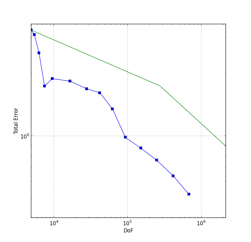
Figure 1: Total error for uniform (green line) and adaptive mesh refinement (blue line).

DoF	Error in $H$	Error in $j$	Total Error	$\mathcal{M}_{h}$
$4940$	$0.864259760285$	$3.15539577688$	$3.2716154178$	$63.4376616999$
$5436$	$0.694612463498$	$3.02692021715$	$3.10559695959$	$58.5220353976$
$6280$	$0.560747440261$	$2.46658970377$	$2.52952613319$	$46.1596277893$
$7480$	$0.517270941002$	$1.66980235746$	$1.74808728025$	$29.9835458365$
$9506$	$0.486958908788$	$1.83890409144$	$1.90228736955$	$33.7781950898$
$16593$	$0.409942119878$	$1.79996131396$	$1.8460534319$	$27.7781692767$
$27622$	$0.322357401619$	$1.66560722229$	$1.69651457799$	$22.1793926139$
$42000$	$0.284583422125$	$1.59619732314$	$1.62136782334$	$20.1292192945$
$62424$	$0.234023588085$	$1.33186688758$	$1.35227084788$	$16.7472327351$
$92730$	$0.196145507066$	$0.963057265783$	$0.982828752692$	$12.4090773249$
$150802$	$0.166713389106$	$0.857068785338$	$0.873132439501$	$10.621022309$
$248269$	$0.143328090061$	$0.747991599295$	$0.761599877899$	$9.09719391479$
$414395$	$0.120042829228$	$0.630681094598$	$0.642003834827$	$7.62309929568$
$674856$	$0.102521829252$	$0.510228751611$	$0.520426848311$	$6.30611525921$

Table 1: Convergence history.

In Figure 2, we plot the finest mesh as the result of the adaptive method. It is noticeable that the adaptive mesh refinement is mainly concentrated in the control domain. Moreover, the computed optimal control and optimal magnetic field are depicted in Figure 3. We see that they are already close to the optimal one.

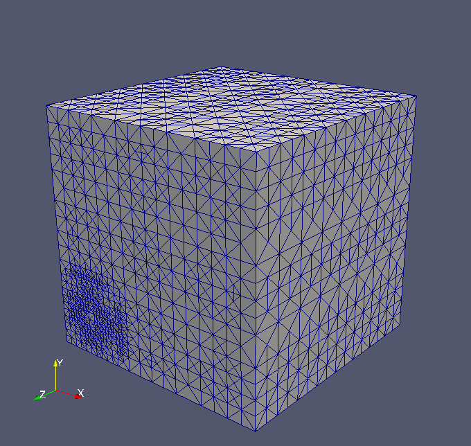
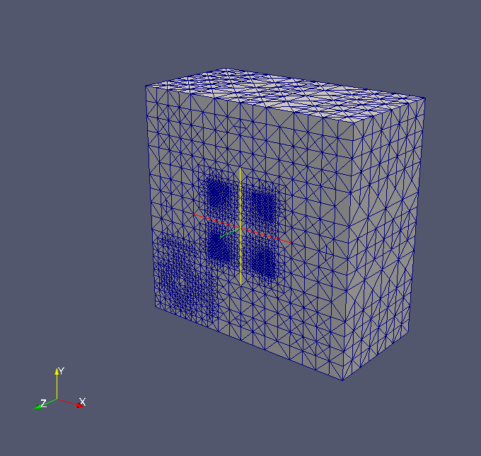
Figure 2: Adaptive mesh.

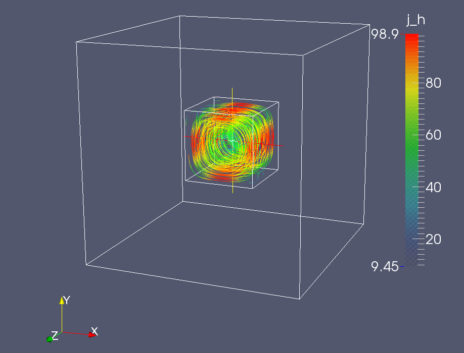
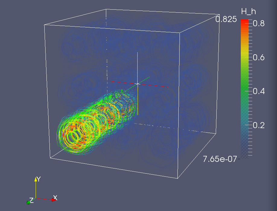
Figure 3: Computed optimal control (left plot) and optimal magnetic field (right plot) on the finest adaptive mesh.

In our second test, we carried out a numerical experiment by making use of the exact total error $|||(\bar{H}-\bar{H}_{h},\bar{j}-\bar{j}_{h})|||$ as the estimator (exact estimator) in the adaptive mesh refinement. More precisely, we replaced $\mathcal{M}_{T}$ in the Dörfler marking strategy (7.14) by the exact total error over each element $T\in\mathcal{T}_{h}(\Omega)$. Figure 4 depicts the computed total error resulting from this adaptive technique compared with our method. Here, the convergence performance of the mesh refinement strategy using the exact estimator turns out to be quite similar to the one based on the estimator $\mathcal{M}_{h}$. Also, the resulting adaptive meshes from these two methods exhibit a similar structure, see Figure 5. Based on these numerical results, we finally conclude that the proposed a posteriori estimator $\mathcal{M}_{h}$ is indeed suitable for an adaptive mesh refinement strategy, in order to improve the convergence performance of the finite element solution towards the optimal one.

DoF	Error in $H$	Error in $j$	Total Error
$4940$	$0.864259760285$	$3.15539577688$	$3.2716154178$
$5372$	$0.700582925336$	$3.0269236357$	$3.10694112137$
$5956$	$0.567880369596$	$2.59095417982$	$2.65245766717$
$6866$	$0.525899386428$	$1.65477728914$	$1.73633465706$
$7975$	$0.491051451195$	$1.79991321699$	$1.86569534395$
$13420$	$0.475834638164$	$1.68710457122$	$1.75292339739$
$21122$	$0.469036197488$	$1.76583157736$	$1.82706215389$
$31404$	$0.459163475711$	$1.65610319012$	$1.71857757281$
$44722$	$0.438814299362$	$1.41717667783$	$1.48355914123$
$62092$	$0.377265302988$	$1.09347162408$	$1.15672351991$
$88972$	$0.297757792322$	$0.883606131143$	$0.932426671584$
$129694$	$0.268987264855$	$0.837765084641$	$0.879888905316$
$215804$	$0.208852836651$	$0.721694386498$	$0.751307057654$
$334072$	$0.194097809391$	$0.587416582193$	$0.618653538457$
$538189$	$0.157893445276$	$0.494322025147$	$0.518926396136$

Table 2: Convergence history for the adaptive refinement using the exact estimator.

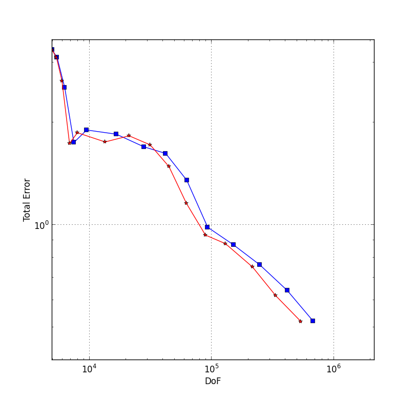
Figure 4: Total error for the adaptive refinement strategies based on the exact estimator (red line) and the estimator $\mathcal{M}_{h}$ (blue line).

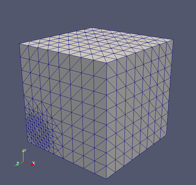
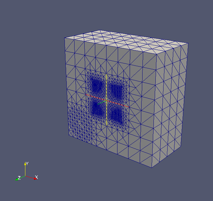
Figure 5: Adaptive mesh resulting from the estimator $\mathcal{M}_{h}$ (upper plot) and the exact estimator (lower plot).

References

- [1] S. Bauer, D. Pauly, and M. Schomburg. The Maxwell compactness property in bounded weak Lipschitz domains with mixed boundary conditions. SIAM J. Math. Anal., 2016.
- [2] M. Bebendorf. A note on the Poincaré inequality for convex domains. Z. Anal. Anwendungen, 22(4):751–756, 2003.
- [3] W. Dörfler. A convergent adaptive algorithm for Poisson’s equation. SIAM J. Numer. Anal., 33(3):1106–1124, 1996.
- [4] V. Girault and P.-A. Raviart. Finite Element Methods for Navier-Stokes Equations: Theory and Algorithms. Springer (Series in Computational Mathematics), Heidelberg, 1986.
- [5] R. Hiptmair. Finite elements in computational electromagnetism. Acta Numer., 11:237–339, 2002.
- [6] R. H. W. Hoppe and I. Yousept. Adaptive edge element approximation of H(curl)-elliptic optimal control problems with control constraints. BIT, 55(1):255–277, 2015.
- [7] F. Jochmann. A compactness result for vector fields with divergence and curl in involving mixed boundary conditions. Appl. Anal., 66:189–203, 1997.
- [8] M. Kolmbauer and U. Langer. Efficient solvers for some classes of time-periodic eddy current optimal control problems. In Oleg P. Iliev, Svetozar D. Margenov, Peter D Minev, Panayot S. Vassilevski, and Ludmil T Zikatanov, editors, Numerical Solution of Partial Differential Equations: Theory, Algorithms, and Their Applications, volume 45, pages 203–216. Springer New York, 2013.
- [9] M. Kolmbauer and U. Langer. A robust preconditioned MinRes solver for time-periodic eddy current problems. Comput. Methods Appl. Math., 13(1):1–20, 2013.
- [10] R. Leis. Initial Boundary Value Problems in Mathematical Physics. Teubner, Stuttgart, 1986.
- [11] A. Logg, K.-A. Mardal, and G. N. Wells. Automated Solution of Differential Equations by the Finite Element Method. Springer, Boston, 2012.
- [12] J.-C. Nédélec. Mixed finite elements in . Numer. Math., 35(3):315–341, 1980.
- [13] P. Neittaanmäki and S. Repin. Reliable methods for computer simulation, error control and a posteriori estimates. Elsevier, New York, 2004.
- [14] S. Nicaise, S. Stingelin, and F. Tröltzsch. On two optimal control problems for magnetic fields. Computational Methods in Applied Mathematics, 14(4):555–573, 2014.
- [15] S. Nicaise, S. Stingelin, and F. Tröltzsch. Optimal control of magnetic fields in flow measurement. Discrete Contin. Dyn. Syst. Ser. S, 8(3):579–605, 2015.
- [16] D. Pauly. On constants in Maxwell inequalities for bounded and convex domains. Zapiski POMI, 435:46-54, 2014, & J. Math. Sci. (N.Y.), 2014.
- [17] D. Pauly. On Maxwell’s and Poincaré’s constants. Discrete Contin. Dyn. Syst. Ser. S, 8(3):607–618, 2015.
- [18] D. Pauly. On the Maxwell constants in 3D. Math. Methods Appl. Sci., 2015.
- [19] D. Pauly and S. Repin. Two-sided a posteriori error bounds for electro-magneto static problems. J. Math. Sci. (N.Y.), 166(1):53–62, 2010.
- [20] L.E. Payne and H.F. Weinberger. An optimal Poincaré inequality for convex domains. Arch. Rational Mech. Anal., 5:286–292, 1960.
- [21] R. Picard. An elementary proof for a compact imbedding result in generalized electromagnetic theory. Math. Z., 187:151–164, 1984.
- [22] R. Picard, N. Weck, and K.-J. Witsch. Time-harmonic Maxwell equations in the exterior of perfectly conducting, irregular obstacles. Analysis (Munich), 21:231–263, 2001.
- [23] S. Repin. A posteriori estimates for partial differential equations. Walter de Gruyter (Radon Series Comp. Appl. Math.), Berlin, 2008.
- [24] F. Tröltzsch and A. Valli. Optimal control of low-frequency electromagnetic fields in multiply connected conductors. To appear in Optimization, DOI:10.1080/02331934.2016.1179301.
- [25] F. Tröltzsch and I. Yousept. PDE-constrained optimization of time-dependent 3D electromagnetic induction heating by alternating voltages. ESAIM Math. Model. Numer. Anal., 46(4):709–729, 2012.
- [26] C. Weber. A local compactness theorem for Maxwell’s equations. Math. Methods Appl. Sci., 2:12–25, 1980.
- [27] N. Weck. Maxwell’s boundary value problems on Riemannian manifolds with nonsmooth boundaries. J. Math. Anal. Appl., 46:410–437, 1974.
- [28] K.-J. Witsch. A remark on a compactness result in electromagnetic theory. Math. Methods Appl. Sci., 16:123–129, 1993.
- [29] Y. Xu and J. Zou. A convergent adaptive edge element method for an optimal control problem in magnetostatics. To appear in ESAIM: M2AN, DOI: http://dx.doi.org/10.1051/m2an/2016030, 2006.
- [30] K. Yosida. Functional Analysis. Springer, Heidelberg, 1980.
- [31] I. Yousept. Finite Element Analysis of an Optimal Control Problem in the Coefficients of Time-Harmonic Eddy Current Equations. Journal of Optimization Theory and Applications, 154(3):879–903, 2012.
- [32] I. Yousept. Optimal control of Maxwell’s equations with regularized state constraints. Computational Optimization and Applications, 52(2):559–581, 2012.
- [33] I. Yousept. Optimal Control of Quasilinear -Elliptic Partial Differential Equations in Magnetostatic Field Problems. SIAM J. Control Optim., 51(5):3624–3651, 2013.