Enumerating secondary structures and structural moieties for circular RNAs

Abstract

A quantitative characterization of the relationship between molecular sequence and structure is essential to improve our understanding of how function emerges. This particular genotype-phenotype map has been often studied in the context of RNA sequences, with the folded configurations standing as a proxy for the phenotype. Here, we count the secondary structures of circular RNAs of length $n$ and calculate the asymptotic distributions of different structural moieties, such as stems or hairpin loops, by means of symbolic combinatorics. Circular RNAs differ in essential ways from their linear counterparts. From the mathematical viewpoint, the enumeration of the corresponding secondary structures demands the use of combinatorial techniques additional to those used for linear RNAs. The asymptotic number of secondary structures for circular RNAs grows as $a^{n}n^{-5/2}$, with $a$ depending on particular constraints applied to the secondary structure. As it occurs with linear RNA, the abundance of any structural moiety is normally distributed in the limit $n\to\infty$, with a mean and a variance that increase linearly with $n$.

1 Introduction

Notwithstanding the important role that selection has traditionally played in evolutionary theory, evolution is not possible if selection has not variation to act upon. Thus mutations —widely understood as imperfect replications— are the fuel to evolutionary dynamics. But mutations act at the level of the genotype whereas selection acts at the level of the phenotype —the physical manifestation of the genotype—, and the translation from one to the other —the so-called genotype-phenotype (GP) map— is far from trivial [1]. Most mutations have no effect on the phenotype (they are neutral), whereas occasionally a mutation has a dramatic (mostly deleterious but sometimes beneficial) phenotypic effect. Thus, evolutionary dynamics is critically affected by the structure of the GP map [2].

Understanding the GP map is a challenge for the evolutionary community, overall because addressing this problem in real systems is of an overwhelming complexity. Accordingly, several simplified models have been studied to gain insights into this difficult issue [3]. Computationally tractable models incorporate only a few levels among those involved in an actual GP map. They have considered protein folding [4, 5] or protein aggregation [6] at basic molecular levels, and gene-regulatory [7] or metabolic [8] networks at higher functional levels. Recent models encompass different levels at the same time [9]: In contrast with simple sequence-structure GP maps, the inclusion of different levels from genotype to phenotype permits the emergence of properties such as environment-dependent molecular function.

Pioneer among those models was the folding of sequences of RNA into their secondary structure —taken as a proxy for function [10, 11], which likely represents the most studied GP map to date. Folding is driven by base pair stacking mainly and also by the formation of hydrogen bonds between CG, AU, and GU base pairs, and the secondary structure of the molecule is determined by its minimum free-energy configuration. Despite its apparent simplicity and the inherent impossibility to capture all features of natural GP relationships, RNA sequence-to-secondary structure maps have properties shared by all GP maps studied to date, as the relationship between the number of genotypes yielding the same phenotype and the neutrality of the latter [12, 13].

An important question in characterizing this GP map is how many different secondary structures an RNA molecule $n$ base pairs long can form. That problem was solved long ago, with the help of recurrence equations and subsequent generating functions, for several variants of the model [14, 15, 16]. Asymptotic expressions were provided when $n$ is large under different constraints imposed to the secondary structure —such as having a minimum number of unpaired nucleotides in hairpin loops or stems of a minimal given length. Another relevant question, which represents a step forward in the relation between structure and function, is how many secondary structures present particular structural moieties [17, 18]. A prominent example is that of short sequences with hairpin loops, which have been shown to act as ribozymes with ligase catalytic activity under general conditions [19]. This undemanding phenotype-to-function map could have been essential in the emergence of RNA molecules with complex activity in a prebiotic RNA world [20]. Beyond characterizing the GP map, having closed-form expressions for the number of RNA structures with specific structural moieties is important when comparing structure formation by natural sequences with that of shuffled versions of the same sequence [21, 22].

The distribution of the number of different structural motifs (stems and hairpin loops among others) in the limit of $n$ large has been shown to converge to a Gaussian in the limit of large $n$ [23, 24]. Two different techniques employed to reach that goal are symbolic methods introduced in modern combinatorics [25], as in [23], and Knudsen-Hein stochastic context-free grammars [26], as in [24]. In an exhaustive work [23], Reidys tackled in depth the properties of RNA folded structures bearing a type of tertiary interactions known as pseudoknots. The functional form of the number of structures with pseudoknots as a function of sequence length $n$ is of the general form $a^{n}n^{-b}$, with $a\in\mathbb{R}^{+}$ and $b\in\mathbb{Q}^{+}$ —their values depending on restrictions put on the folded structure. An important constraint is the complexity of pseudoknots, which conditions the mathematical description of the problem. Specifically, folded RNA molecules are first reduced to a core skeleton containing information only on the pseudoknot architecture of the fold. Generating functions for the number of possible alternative core structures with the previous architecture are derived and, subsequently, full folds are recovered by reintroducing stems and unpaired nucleotides in all possible compatible positions —through composition of suitably defined generating functions. Eventually, the total number of structures with the required pseudoknot properties and other possible structural constraints is obtained. Further details can be found in [23]. This tricky procedure for structures with pseudoknots is not necessary in the case of plain secondary structures, as we show here. Application of symbolic combinatorics to the latter case serves as an introduction to the calculation of the number of secondary structures for circular RNA sequences. As will be shown, particular properties of circular RNA demand the introduction of combinatorial techniques beyond those needed to enumerate open RNA sequences —with or without pseudoknots.

Circular RNAs form covalently closed continuous loops with specific properties that distinguish them from linear RNAs. Among others, circular RNAs are small and non-coding in most cases, and have higher resistance to exonuclease-mediated degradation and higher structural stability. Viroids, first described half a century ago [27], are a relevant example of circular RNA. These pathogenic, naked RNA molecules of a few hundred nucleotides in length infect plants, occasionally causing strong symptoms. The mechanisms implied in cell entry, replication and propagation are still partly unknown. Viroids present secondary structures with highly conserved regions that fall within two structural classes: rod-like and branched folds. The secondary structure of viroids plays an essential role in chemical function [28] and acts as a buffer to control the structural effect of point mutations [29]. Virusoids are another class of circular RNAs that depend on helper viruses for replication and encapsidation. They are related to viroids, though virusoids code for some proteins. Two interesting examples in this class of hyperpathogens are Hepatitis delta virus [30] and the smallest known circular RNA in the viroid-virusoid class, with 220nt [31]. As in viroids, the secondary structure of virusoids is highly compact and constrained by function. Circular RNAs encoded in animal genomes, on the other hand, are currently a hot topic [32]. Indeed, recent studies report a previously unsuspected abundance of circular RNAs, which awakes the hunch that they must play main functional roles in the cell [33]. While some of those circular RNAs have gene regulatory activity, the function performed by thousand of others is as yet unknown [32, 34]. Therefore, a theoretical understanding of the structural diversity of secondary structures of circular RNAs appears as a timely endeavor, further considering that closed RNA sequences have folding restrictions different from those of their linear counterparts. Formal studies on the folding properties of circular RNAs are limited, to the best of our knowledge, to the case of symmetric sequences [35], whose contribution to the total number of sequences and folds asymptotically vanishes as $n$ grows. As we demonstrate here, specific properties of circular RNA entail a comparatively lower number of secondary structures and lead to different asymptotic behavior.

The paper is organized as follows. Section 2 briefly introduces those aspects of the symbolic method [25] relevant for our study. In Section 3.1 we derive the generating function for the number of secondary structures with stems of length at least $s$ and hairpins with at least $m$ unpaired nucleotides, and recover the known expressions in the limit $n\to\infty$. Section 3.2 contains the calculation of the frequency of structures with a given number of base pairs and is followed by the simultaneous count of the number of hairpins in Section 3.3. The method extends to multivariate analysis suitable for counting combinatorial structures with any number of constraints, in agreement with results obtained in [24]. Though these sections mostly review results that in one or another form can be found in the mathematics literature, we believe it is convenient to rephrase certain aspects that are later used, in order to convey a biological intuition of how calculations are performed and to make this work self-contained. Section 3.4 introduces the main novelty of this work, that is, the enumeration of secondary structures in circular RNAs, followed by a derivation of the distributions of base pairs and hairpins as a function of $n$ in Section 3.5. We close with a brief discussion.

2 Methods

A full account of symbolic methods in combinatorics can be found in Part A of Ref. [25]. We provide a very brief account in this section. Readers familiar with this method can safely skip this section.

A combinatorial class $\mathcal{A}$ will be a set of elements on which a size function $|\cdot|$ is defined. The counting problem is to obtain $a_{n}$, the number of elements $a\in\mathcal{A}$ such that $|a|=n$. A related problem is to obtain the generating function

$$A(z)=\sum_{n}a_{n}z^{n}=\sum_{a\in\mathcal{A}}z^{|a|}$$ (1)

($n$ runs on all possible sizes) whose coefficients yield the sequence $\{a_{n}\}$. The second writing for $A(z)$ turns out to be very useful when thinking about these problems, because it means that every element of $\mathcal{A}$ contributes to the sum defining $A(z)$ with as many factors $z$ as its size.

If a second function is defined on the elements of $\mathcal{A}$, namely $\varphi(a)=l$ (representing any other feature of $a$), we can introduce the bivariate generating function

$$A(z,u)=\sum_{n}\sum_{l}a_{n,l}z^{n}u^{l}=\sum_{a\in\mathcal{A}}z^{|a|}u^{\varphi(a)}.$$ (2)

Clearly $a_{n,l}$ counts the number of elements in $\mathcal{A}$ of size $n$ and feature value $l$, and the second writing can be interpreted as every element $a\in\mathcal{A}$ adding to the generating function —besides the factor $z^{n}$— as many factors $u$ as the value of the feature.

We can combine combinatorial classes to obtain new combinatorial classes. We first have the combinatorial product $\mathcal{C}=\mathcal{A}\times\mathcal{B}$, which is the set made of the ‘composite objects’ $ab$, where $a\in\mathcal{A}$ and $b\in\mathcal{B}$ (notice that $ab$ and $ba$ are in general different objects). The size of the set $\mathcal{C}$ is defined as $|ab|=|a|+|b|$ (the size of the composite object is the sum of the sizes of the components). Accordingly,

$$C(z)=\sum_{c\in\mathcal{C}}z^{|c|}=\sum_{a\in\mathcal{A}}\sum_{b\in\mathcal{B}}z^{|ab|}=\sum_{a\in\mathcal{A}}\sum_{b\in\mathcal{B}}z^{|a|+|b|}=A(z)B(z).$$ (3)

Another operation is the combinatorial sum, $\mathcal{C}=\mathcal{A}+\mathcal{B}$, also referred to as disjoint union. $\mathcal{C}$ is the union of $\mathcal{A}$ and $\mathcal{B}$ provided the elements of these two sets are distinguishable (in other words, it is as if we paint the elements of these two sets with two different colors and then make the union of them both). Therefore $c\in\mathcal{C}$ is either an element of $\mathcal{A}$ or an element of $\mathcal{B}$ and inherits the corresponding size. Hence,

$$C(z)=\sum_{c\in\mathcal{C}}z^{|c|}=\sum_{a\in\mathcal{A}}z^{|a|}+\sum_{b\in\mathcal{B}}z^{|b|}=A(z)+B(z).$$ (4)

There are further more complex operations with combinatorial classes. Thus

$$\mathcal{C}=\mathsf{SEQ}(\mathcal{A}):=\mathcal{E}+\mathcal{A}+\mathcal{A}\times\mathcal{A}+\mathcal{A}\times\mathcal{A}\times\mathcal{A}+\cdots,$$ (5)

where $\mathcal{E}=\{\varepsilon\}$, the class made of the null element alone ($|\varepsilon|=0$), is referred to as the sequence of $\mathcal{A}$, i.e., the combinatorial class made of the null element, plus all elements of $\mathcal{A}$, plus all pairs of elements of $\mathcal{A}$, and so on. By applying the transformation rules for the sum and the product

$$C(z)=1+A(z)+A(z)^{2}+A(z)^{3}+\cdots=\frac{1}{1-A(z)}.$$ (6)

Sequences can be constrained to have composite elements just of certain specific compositions. For instance, $\mathsf{SEQ}_{k}(\mathcal{A}):=\mathcal{A}\times\mathcal{A}\times\cdots\times\mathcal{A}$ ($k$ times) is restricted to sequences made of exactly $k$ elements of $\mathcal{A}$ —its generating function being $A(z)^{k}$. Likewise

$$\begin{split}\mathcal{C}_{\geqslant k}&=\mathsf{SEQ}_{\geqslant k}(\mathcal{A})=\sum_{j=k}^{\infty}\mathsf{SEQ}_{k}(\mathcal{A}),\\ \mathcal{C}_{<k}&=\mathsf{SEQ}_{<k}(\mathcal{A})=\sum_{j=0}^{k-1}\mathsf{SEQ}_{k}(\mathcal{A}),\end{split}$$ (7)

define sequences containing at least $k$ and less than $k$ elements of $\mathcal{A}$ respectively. Then

$$\begin{split}C_{\geqslant k}(z)&=\frac{A(z)^{k}}{1-A(z)},\\ C_{<k}(z)&=1+A(z)+A(z)^{2}+\cdots+A(z)^{k-1}\\ &=\frac{1-A(z)^{k}}{1-A(z)},\end{split}$$ (8)

are their corresponding generating functions.

Other interesting operations with combinatorial classes are power sets ($\mathsf{PSET}$), multisets ($\mathsf{MSET}$), and cycles ($\mathsf{CYC}$) [25].

$\mathsf{PSET}(\mathcal{A})$ is the class whose members are made of subsets of elements of $\mathcal{A}$. Thus

$$\mathcal{C}=\mathsf{PSET}(\mathcal{A}):=\prod_{a\in\mathcal{A}}\big{(}\mathcal{E}+\{a\}\big{)}$$ (9)

and therefore

$$\begin{split}C(z)&=\prod_{a\in\mathcal{A}}\left(1+z^{|a|}\right)=\prod_{n=1}^{\infty}\left(1+z^{n}\right)^{a_{n}}\\ &=\exp\left\{\sum_{k=1}^{\infty}\frac{(-1)^{k+1}}{k}A\big{(}z^{k}\big{)}\right\}.\end{split}$$ (10)

(The last step follows by writing the product as the exponential of a sum of logarithms and then Taylor-expanding those logarithms.)

$\mathsf{MSET}(\mathcal{A})$ is the class whose members are made of sequences of arbitrary length of elements of $\mathcal{A}$. Thus

$$\mathcal{C}=\mathsf{MSET}(\mathcal{A}):=\prod_{a\in\mathcal{A}}\mathsf{SEQ}\big{(}\{a\}\big{)}$$ (11)

and therefore

$$\begin{split}C(z)&=\prod_{a\in\mathcal{A}}\left(1-z^{|a|}\right)^{-1}=\prod_{n=1}^{\infty}\left(1-z^{n}\right)^{-a_{n}}\\ &=\exp\left\{\sum_{k=1}^{\infty}\frac{1}{k}A\big{(}z^{k}\big{)}\right\}.\end{split}$$ (12)

$\mathsf{CYC}(\mathcal{A})$ is the class whose members are made of circular sequences of arbitrary length of elements of $\mathcal{A}$. The derivation of the generating function of $\mathcal{C}=\mathsf{CYC}(\mathcal{A})$ is more involved [25, §A.4], but can be written in terms of Euler’s totient function $\varphi(k)$ as

$$C(z)=-\sum_{k=1}^{\infty}\frac{\varphi(k)}{k}\log\left[1-A\big{(}z^{k}\big{)}\right].$$ (13)

One last class we will need is $\mathsf{MSET}_{2}(\mathcal{A})=\mathsf{CYC}_{2}(\mathcal{A})$, whose members are pairs of elements of $\mathcal{A}$ regardless of the order (when the order matters the class is $\mathcal{A}\times\mathcal{A}$). There are many ways to obtain its corresponding generating function, but perhaps the easiest is to first introduce $\mathsf{DIAG}(\mathcal{A})$, the class of pairs of identical elements of $\mathcal{A}$. Its corresponding generating function is $A\big{(}z^{2}\big{)}$ —because it contains one element per element of $\mathcal{A}$, but its size is double. Then, $\mathcal{C}=\mathsf{CYC}_{2}(\mathcal{A}):=\frac{1}{2}\big{[}\mathcal{A}\times\mathcal{A}+\mathsf{DIAG}(\mathcal{A})\big{]}$, and its generating function will be

$$C(z)=\frac{1}{2}\big{[}A(z)^{2}+A\big{(}z^{2}\big{)}\big{]}.$$ (14)

Further classes and development can be found in [25].

By way of illustration, consider the class $\mathcal{T}$ of all binary trees with $n$ interior nodes. This class contains the tree with no interior nodes $\mathcal{E}$ plus all trees made of a root node $\mathcal{U}=\{\bullet\}$ from which two new trees of $\mathcal{T}$ hang. Thus

$$\mathcal{T}=\mathcal{E}+\mathcal{T}\times\mathcal{U}\times\mathcal{T}.$$ (15)

The size of the tree in $\mathcal{E}$ is zero, whereas the root node $\mathcal{U}$ —obviously interior— contributes $z$ to $T(z)$. Therefore (15) translates into $T(z)=1+zT(z)^{2}$, whence

$$T(z)=\frac{1-\sqrt{1-4z}}{2z}=\sum_{n=0}^{\infty}\frac{1}{n+1}\binom{2n}{n}z^{n},$$ (16)

the generating function of Catalan’s numbers. A nice property of generating functions is that we do not need to know the coefficients to obtain their asymptotic expression. For that we can resort to an extension of Darboux’s theorem [25, 17]:

Theorem 1 (Darboux)

Let $f(z)=\sum\limits_{n=0}^{\infty}f_{n}z^{n}$, with $f_{n}\geqslant 0$, be an analytic function in the circle $|z|<\zeta$ of the form

$$f(z)=g(z)+h(z)\left(1-\frac{z}{\zeta}\right)^{\alpha}+O\left(\left(1-\frac{z}{\zeta}\right)^{\alpha+1}\right),\quad\alpha\notin\mathbb{N},$$ (17)

where $g(z)$ and $h(z)$ are analytic around $\zeta$. Then, as $n\to\infty$,

$$f_{n}=\frac{h(\zeta)}{\Gamma(-\alpha)}n^{-1-\alpha}\zeta^{-n}\left[1+O\left(n^{-1}\right)\right].$$ (18)

Applied to $T(z)$, Darboux’s theorem implies $t_{n}=4^{n}/\sqrt{\pi n^{3}}+O\left(n^{-5/2}\right)$ as $n\to\infty$.

3 Results

3.1 Counting secondary structures in RNA

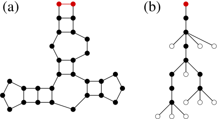
Figure 1: Tree representation of the secondary structure of RNA sequences. (a) Secondary structure of an RNA sequence that starts with a stem. Stems cannot contain less that two pairs of bases, and hairpin loops cannot be made of less than three bases. (b) Tree representation of the structure in (a). Filled circles represent paired bases; empty circles stand for unpaired bases. For the sake of clarity, the root of the tree in (b) and the corresponding base pair in the secondary structure (a) are colored.

Figure 1(a) illustrates one possible secondary structure for an RNA molecule $n=30$ bases long. Some bases are complementary and can pair up forming a hydrogen bond, some others are not and remain unbound. Sequences of contiguous paired bases form stems; unpaired bases form loops of different kinds (hairpins, bulges, mutiloops, interior loops…). A description of these structures along with an illustration of them can be found in [17].

Determining the specific secondary structure of an RNA molecule is a complex problem that requires not only a careful energetic minimization, but also considerations on the environmental conditions and folding kinetics, among others [36]. However, some folding constraints arise as a consequence of local conditions for energetic stability. Among them, two are especially important and were taken into account in early calculations of the number of realistic RNA secondary structures [11]. Here we use two general assumptions in agreement with those restrictions: (1) no stem can contain less than $s$ pairs, and (2) no hairpin loop can contain less than $m$ bases. This notwithstanding, the combinatorial calculations we will be performing here disregard any further energetic constraints, so the estimation provided by this method is only an upper bound to the true number of feasible structures —because some structures are forbidden on energetic grounds. The same holds for the circular RNA structures that we will compute later.

We will divide our counting problem in two steps. First, we will count those foldings starting with a stem —as the one illustrated in Figure 1(a). Second, we will take into account that a general folding consists of several of the former ones joined by free chains —possibly with chains also at the beginning and/or at the end.

A tree representation of the folding turns out to be more suitable for the symbolic method. In this representation stems appear as chains of filled dots ($\bullet$) and loops are represented as branches containing an empty dot ($\circ$) per unpaired base and a chain of filled dots per stem branching off the loop (see Figure 1(b)).

Let $\mathcal{B}$ denote the combinatorial class of all trees representing an RNA secondary structure starting with a stem and subject to the two above constraints. Then

$$\mathcal{B}=\mathsf{SEQ}_{\geqslant s}\big{[}\{\bullet\}\big{]}\times\left(\mathsf{SEQ}\big{[}\{\circ\}+\mathcal{B}\big{]}-\mathcal{B}-\mathsf{SEQ}_{<m}[\{\circ\}]\right).$$ (19)

The first factor $\mathsf{SEQ}_{\geqslant s}\big{[}\{\bullet\}\big{]}$ stands for the sequence of $\bullet$ from the root of the tree to the first branching point. This sequence must have at least $s$ $\bullet$, but its length is otherwise unlimited —hence the $\mathsf{SEQ}_{\geqslant s}$ operator. What one can find at the first branching event is described by the next factor $\mathsf{SEQ}\big{[}\{\circ\}+\mathcal{B}\big{]}-\mathcal{B}-\mathsf{SEQ}_{<m}[\{\circ\}]$. The first SEQ operator means that the number of branches is arbitrary and each branch can either be a $\circ$ or another tree from the class $\mathcal{B}$ —hence the argument $\{\circ\}+\mathcal{B}$. Finally, the term $-\mathcal{B}-\mathsf{SEQ}_{<m}[\{\circ\}]$ excludes branchings that are not allowed: there can be neither a single $\mathcal{B}$ branch —that would mean extending the previous stem— nor less than $m$ $\circ$ and nothing else —that would mean a hairpin loop with less than $m$ unpaired bases.

Let $B(z)=\sum_{n=0}^{\infty}b_{n}z^{n}$ be the generating function of $b_{n}$, the number of different $n$-long secondary structures starting with a stem. Since every $\circ$ (unbounded base) in (19) contributes $z$ to $B(z)$ and every $\bullet$ (pair of bonded bases) contributes $z^{2}$ to $B(z)$, we can translate (19) as

$$B(z)=\frac{z^{2s}}{1-z^{2}}\left(\frac{1}{1-z-B(z)}-B(z)-T_{m}(z)\right),$$ (20)

where $T_{m}(z)=1+z+\cdots+z^{m-1}$ is the generating function of $\mathsf{SEQ}_{<m}[\{\circ\}]$.

Once we have characterized the class $\mathcal{B}$, the class of possible RNA foldings $\mathcal{R}$ can be constructed as

$$\mathcal{R}=\mathsf{SEQ}\big{[}\{\circ\}+\mathcal{B}\big{]},$$ (21)

i.e., a sequence of arbitrary length (including $n=0$) each of whose components is either an unpaired base ($\circ$) or a folded structure from $\mathcal{B}$. In terms of generating functions,

$$R(z)=\frac{1}{1-z-B(z)},$$ (22)

where $R(z)=\sum_{n=0}^{\infty}r_{n}z^{n}$, $r_{n}$ being the number of different $n$-long RNA secondary structures. Eliminating $B(z)$ in this equation and substituting into (20) leads to the quadratic equation

$$z^{2s}R(z)^{2}-\big{[}(1-z)(1-z^{2}+z^{2s})+z^{2s}T_{m}(z)\big{]}R(z)+1-z^{2}+z^{2s}=0,$$ (23)

whose solution is

$$R(z)= \frac{(1-z)(1-z^{2}+z^{2s})+z^{2s}T_{m}(z)-\Delta(z)^{1/2}}{2z^{2s}},$$ (24)

$$\Delta(z):= \big{[}(1-z)(1-z^{2}+z^{2s})+z^{2s}T_{m}(z)\big{]}^{2}$$

$$-4z^{2s}(1-z^{2}+z^{2s}).$$ (25)

This is Eq. (43) of Ref. [17] (beware of a missing factor $2$ in the left-hand side of that equation).

Suppose $z_{*}$ is the (single) root of $\Delta(z)$ with the smallest absolute value. Then $\Delta(z)=(z_{*}-z)Q(z)$ and the singular part of $R(z)$ will have the form

$$-\frac{[z_{*}Q(z)]^{1/2}}{2z^{2s}}\left(1-\frac{z}{z_{*}}\right)^{1/2}.$$ (26)

Thus, applying Darboux’s theorem we can conclude

$$r_{n}=\frac{C_{s}}{2\sqrt{\pi n^{3}}}z_{*}^{-n}\left[1+O\left(\frac{1}{n}\right)\right],\quad C_{s}:=\frac{Q(z_{*})^{1/2}}{2z_{*}^{2s-1/2}}.$$ (27)

For $s=2$, $m=3$ we obtain $z_{*}=0.540857\dots$ and $C_{2}=5.263602\dots$, leading to the well-known result [17, Table 1] $r_{n}\sim 1.48483n^{-3/2}(1.84892)^{n}$.

3.2 Asymptotic distribution of the number of base pairs

Now we aim to obtain the asymptotic behavior, when $n,l\to\infty$, of the distribution $p_{n,l}:=r_{n,l}/r_{n}$, where $r_{n,l}$ counts the number of RNA secondary structures having exactly $l$ base pairs. The symbolic method is easily adapted to obtain $p_{n,l}$. To this end we need to introduce the bivariate generating functions

$$R(z,w)=\sum_{n=0}^{\infty}\sum_{l=0}^{\infty}r_{n,l}z^{n}w^{l},\quad B(z,w)=\sum_{n=0}^{\infty}\sum_{l=0}^{\infty}b_{n,l}z^{n}w^{l},$$ (28)

where $b_{n,l}$ counts only secondary structures starting with a stem.

Equations (19) and (21) remain valid, but now every $\circ$ contributes $z$ whereas every $\bullet$ contributes $z^{2}w$ to both generating functions (a $\bullet$ is both two bases and a base pair). Thus, Eqs. (20) and (22) become

$$B(z,w) =\frac{z^{2s}w^{s}}{1-z^{2}w}\left(\frac{1}{1-z-B(z,w)}-B(z,w)-T_{m}(z)\right),$$ (29)

$$R(z,w) =\frac{1}{1-z-B(z,w)},$$ (30)

and we obtain the modified quadratic equation for $R(z,w)$

$$\begin{split}z^{2s}&w^{s}R(z,w)^{2}-\big{[}(1-z)(1-z^{2}w+z^{2s}w^{s})\\ &+z^{2s}w^{s}T_{m}(z)\big{]}R(z,w)+1-z^{2}w+z^{2s}w^{s}=0.\end{split}$$ (31)

We can interpret $R(z,w)$ as the generating function of the sequence of polynomials

$$r_{n}(w):=\sum_{l=0}^{\infty}r_{n,l}w^{l}$$ (32)

(notice that $r_{n,l}=0$ if $l>n/2$) and repeat the arguments of the previous section. Thus, if $z_{*}(w)$ is the root with smallest absolute value of

$$\begin{split}\Delta(z,w):=&\big{[}(1-z)(1-z^{2}w+z^{2s}w^{s})+z^{2s}w^{s}T_{m}(z)\big{]}^{2}\\ &-4z^{2s}w^{s}(1-z^{2}w+z^{2s}w^{s})\end{split}$$ (33)

and $\Delta(z,w)=\big{(}z_{*}(w)-z\big{)}Q(z,w)$, then the singular part of $R(z,w)$ will be

$$-\frac{1}{2z^{2s}w^{s}}(z_{*}(w)-z)^{1/2}Q(z,w)^{1/2},$$ (34)

so Darboux’s theorem implies (when $n\to\infty$)

$$\begin{split}r_{n}(w)&=\frac{C_{s}(w)}{2\sqrt{\pi n^{3}}}z_{*}(w)^{-n}\left[1+O\left(\frac{1}{n}\right)\right],\\ C_{s}(w)&:=\frac{Q\big{(}z_{*}(w),w\big{)}^{1/2}}{2z_{*}(w)^{2s-1/2}w^{s}}.\end{split}$$ (35)

Using this information we can obtain the characteristic function of the probability distribution $p_{n,l}$, for a given $n$, as

$$\phi_{n}(q):=\sum_{l=0}^{\infty}p_{n,l}e^{iql}=\frac{r_{n}\left(e^{iq}\right)}{r_{n}(1)},$$ (36)

which, according to eq. (35), will behave, asymptotically in $n$, as

$$\phi_{n}(q)=A_{s}\left(e^{iq}\right)\left(\frac{z_{*}(1)}{z_{*}\left(e^{iq}\right)}\right)^{n+2s-\frac{1}{2}}\left[1+O\left(\frac{1}{n}\right)\right],$$ (37)

where

$$A_{s}(w):=\frac{1}{w^{s}}\left(\frac{Q\big{(}z_{*}(w),w\big{)}}{Q\big{(}z_{*}(1),1\big{)}}\right)^{1/2}.$$ (38)

The values of $r_{n}(1)$, $z_{*}(1)$, and $Q\big{(}z_{*}(1),1\big{)}$ are those obtained in Section 3.1.

From (37) it follows

$$\begin{split}\log\phi_{n}(q)=&\left(n+2s-\frac{1}{2}\right)\log\left(\frac{z_{*}(1)}{z_{*}\left(e^{iq}\right)}\right)\\ &+\log A_{s}\left(e^{iq}\right)+O\left(\frac{1}{n}\right)\\ =&\mu_{n}iq-\frac{\sigma_{n}^{2}}{2}q^{2}+O(q^{3}).\end{split}$$ (39)

In other words, the distribution $p_{n,l}$ behaves, as $n\to\infty$, as a normal distribution in $l$ with mean $\mu_{n}=\mu n+\mu_{0}+O\left(n^{-1}\right)$ and standard deviation $\sigma_{n}=\sigma n^{1/2}+\sigma_{0}n^{-1/2}+O\left(n^{-3/2}\right)$. The precise values depend on $s$ and $m$. For $s=2$, $m=3$ we obtain $\mu\approx 0.286472\dots$, $\mu_{0}\approx-0.792076\dots$, $\sigma\approx 0.255103\dots$, and $\sigma_{0}\approx 0.247963\dots$ Accordingly, the number of different phenotypes of a sequence of length $n$ with $l$ paired bases is given, in the limit $n,l\to\infty$, by

$$r_{n,l}\sim\frac{r_{n}}{\sqrt{2\pi}\sigma_{n}}e^{-(l-\mu_{n})^{2}/2\sigma_{n}^{2}},$$ (40)

with $r_{n}$ as in (27). Equivalent results were obtained in [23] and [24].

3.3 Counting more than one structural element

In this section we are going to count the number of secondary structures with fixed numbers of base pairs and hairpins. Hairpins are going to be counted with a variable $u$ —each hairpin will contribute $u$ to the generating function. Hairpins are elements of $\mathsf{SEQ}_{\geqslant m}[\{\circ\}]$, so we have to separate them out in (19) and reintroduce them with a mark $u$. In other words, we need to replace $\mathsf{SEQ}_{<m}[\{\circ\}]$ by $\mathsf{SEQ}[\{\circ\}]-u\mathsf{SEQ}_{\geqslant m}[\{\circ\}]$. Since the former gives rise to the term $T_{m}(z)$ in (29), this operation amounts to replacing $T_{m}(z)$ by

$$T_{m}(z,u)=\frac{1-uz^{m}}{1-z}$$ (41)

in this and subsequent equations.

Now, interpreting $R(z,w,u)$ as the generating function of the bivariate polynomials

$$r_{n}(w,u):=\sum_{l=0}^{\infty}\sum_{k=0}^{\infty}r_{n,l,k}w^{l}u^{k},$$ (42)

$r_{n,l,k}$ being the number of RNA secondary structures with $l$ base pairs and $k$ hairpins, we can obtain the asymptotic behavior of the probability distribution $p_{n,l,k}:=r_{n,l,k}/r_{n}$ through that of its characteristic function

$$\phi_{n}(\vec{q})=\frac{r_{n}\left(e^{iq_{p}},e^{iq_{h}}\right)}{r_{n}(1,1)},\qquad\vec{q}:=(q_{p},q_{h}).$$ (43)

Following the procedure explained in the previous section we find

$$\begin{split}\log\phi_{n}(\vec{q})=&\left(n+2s-\frac{1}{2}\right)\log\left(\frac{z_{*}(1,1)}{z_{*}\left(e^{iq_{p}},e^{iq_{h}}\right)}\right)\\ &+\log A_{s}\left(e^{iq_{p}},e^{iq_{h}}\right)+O\left(\frac{1}{n}\right),\end{split}$$ (44)

with

$$A_{s}(w,u):=\frac{1}{w^{s}}\left(\frac{Q\big{(}z_{*}(w,u),w,u\big{)}}{Q\big{(}z_{*}(1,1),1,1\big{)}}\right)^{1/2},$$ (45)

$z_{*}(w,u)$ being the singularity of $R(z,w,u)$ with smallest absolute value, and $Q(z,w,u)$ defined as in (33), (34), with $T_{m}(z)$ replaced by $T_{m}(z,u)$ defined in Eq. (41). If we now identify

$$\log\phi_{n}(\vec{q})=\mu^{p}_{n}iq_{p}+\mu^{h}_{n}iq_{h}-\frac{1}{2}\vec{q}\cdot\mathsf{\Sigma}_{n}\cdot\vec{q}^{\mathsf{T}}+O\left(\|\vec{q}\|^{3}\right),$$ (46)

we obtain the mean vector $(\mu^{p}_{n},\mu^{h}_{n})$ and covariance matrix $\mathsf{\Sigma}_{n}$ of a bivariate normal distribution. For instance, setting $s=2$, $m=3$ we get

$$\begin{split}&\mu_{n}^{p}=(0.286472\dots)n-(0.792076\dots)+O\left(n^{-1}\right),\\ &\mu_{n}^{h}=(0.0378631\dots)n+(0.308604\dots)+O\left(n^{-1}\right),\\ &\mathsf{\Sigma}_{n}^{pp}=(0.0650779\dots)n+(0.126513\dots)+O\left(n^{-1}\right),\\ &\mathsf{\Sigma}_{n}^{hh}=(0.0115908\dots)n+(0.0164609\dots)+O\left(n^{-1}\right),\\ &\mathsf{\Sigma}_{n}^{ph}=(-0.00274347\dots)n+(0.00918949\dots)+O\left(n^{-1}\right).\end{split}$$ (47)

Thus, asymptotically,

$$\begin{split}r_{n,l,k}\sim&\frac{r_{n}}{2\pi|\mathsf{\Sigma}_{n}|^{1/2}}\\ &\times\exp\left\{-\frac{1}{2}(l-\mu^{p}_{n},k-\mu^{h}_{n})\cdot\mathsf{\Sigma}_{n}^{-1}\cdot(l-\mu^{p}_{n},k-\mu^{h}_{n})^{\mathsf{T}}\right\}.\end{split}$$ (48)

Obtaining the marginal distribution of base pairs amounts to setting $q_{h}=0$ in (46). One can easily check that it correspond to the distribution (40). Likewise, the marginal distribution of hairpins follows from setting $q_{p}=0$ in (46). It turns out to be a normal distribution with mean $\mu_{n}^{h}$ and variance $\mathsf{\Sigma}_{n}^{hh}$.

New structural elements can be counted in a similar vein, and their corresponding asymptotic distribution will be multivariate normal distributions whose parameters can be determined as we have done in this section. Analogous results for multivariate distributions of structural motifs can be found in [24].

3.4 Counting secondary structures of circular RNAs

Let now $\mathcal{V}$ denote the combinatorial class containing all secondary structures of circular RNAs. As for open sequences, counting is better done using the tree representation of Fig. 1. If secondary structures of linear sequences are encoded in rooted trees, those of circular sequences, for which any base pair can act as a root, would correspond to unrooted trees. There is an ambiguity though when transforming the rooted tree representation into an unrooted one. The rules to transform structures into trees are directional, as illustrated in Fig. 2. To avoid that we introduce a new type of node, a square, to mark the extremes of all stems meeting at a hairpin, a multiloop, or a bulge. The square is understood to represent a base pair for each stem meeting at it. With this new representation each secondary structure of a circular RNA uniquely determines a tree with two types of inner nodes —filled circles and squares— and empty circles for leaves, regardless of the direction we choose to read the structure.

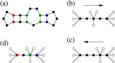
Figure 2: Tree representation of the secondary structure of circular RNAs. (a) Secondary structure of a circular RNA sequence. (b) Tree representation of the structure in (a) as read starting from the leftmost hairpin. (c) Tree representation of the same structure but read from the rightmost hairpin. (d) New tree representation in which square nodes mark the extremes of the stems —hence leaves (empty circles) hang from these nodes. Each square counts one base pair for each stem meeting at it. (Colors are meant to help understand the association between base pairs and square nodes.) Notice that this tree is uniquely defined by the RNA structure regardless of the way we read it.

We will need a new combinatorial class to obtain $\mathcal{V}$, namely

$$\mathcal{B}_{k}=\mathsf{SEQ}_{k}\big{[}\{\bullet\}\big{]}\times\left(\mathsf{SEQ}\big{[}\{\circ\}+\mathcal{B}\big{]}-\mathcal{B}-\mathsf{SEQ}_{<m}[\{\circ\}]\right),$$ (49)

the class of secondary RNA structures starting with a stem of exactly $k$ base pairs. Notice that (19) implies that $\mathcal{B}=\sum_{k\geqslant s}\mathcal{B}_{k}$, and it follows from (19) and (49) that

$$B_{k}(z)=z^{2k-2s}(1-z^{2})B(z).$$ (50)

Counting unrooted trees is a more complicated issue than counting rooted trees. As a matter of fact, the strategy to do it is to reduce the problem to counting rooted trees. This is achieved thanks to a so-called dissymetry theorem that relates both classes of trees [37, §4.1]. If $\mathcal{F}$ denotes a class of rooted trees and $\mathcal{G}$ denotes that of their corresponding unrooted trees, then

$$\mathcal{G}^{\bullet}+\mathcal{G}^{\bullet\!\!-\!\!\bullet}=\mathcal{G}+\mathcal{F}\times\mathcal{F},$$ (51)

where $\mathcal{G}^{\bullet}$ denotes the class of unrooted trees with a marked node, and $\mathcal{G}^{\bullet\!\!-\!\!\bullet}$ denotes the class of unrooted trees with a marked link. In our case, $\mathcal{G}$ stands for $\mathcal{V}$, the class we want to count. As for $\mathcal{F}\times\mathcal{F}$, an analysis of the proof of the theorem reveals that the $\mathcal{F}$s involved arise as a result of removing links in trees of $\mathcal{G}$. Thus, for the kind of trees we aim at counting we need to adapt this result, because links in $\mathcal{V}$ are part of a stem, and stems must have at least $s$ base pairs. Also, as leaves (empty circles) are never the root of a tree, the argument can focus on inner nodes and inner links.

Consider $v\in\mathcal{V}$. Removing an inner link in $v$ yields two trees, one belonging to $\mathcal{B}_{j}$ and another one belonging to $\mathcal{B}_{k}$, such that $j,k\geqslant 1$ and $j+k\geqslant s$. Therefore

$$\mathcal{F}_{s}:=\mathcal{F}\times\mathcal{F}=\sum_{j+k\geqslant s\atop j,k\geqslant 1}\mathcal{B}_{j}\times\mathcal{B}_{k}.$$ (52)

Let us now mark a link of $v$ to transform it into an element of $\mathcal{V}^{\bullet\!\!-\!\!\bullet}$. Two rooted trees from $\mathcal{B}_{j}$ and $\mathcal{B}_{k}$ —with the same index constraints— hang from both sides of the marked link. Since the order of these two trees is irrelevant,

$$\mathcal{V}^{\bullet\!\!-\!\!\bullet}=\frac{1}{2}(\mathcal{F}_{s}+\mathcal{D}_{s}),\qquad\mathcal{D}_{s}:=\sum_{2j\geqslant s}\mathsf{DIAG}(\mathcal{B}_{j}),$$ (53)

using the idea behind the definition of $\mathsf{CYC}_{2}$ (Sec. 2). Finally, if we mark a $\bullet$ node as root, the two hanging branches are one tree from $\mathcal{B}_{j}$ and another one from $\mathcal{B}_{k}$, such that $j,k\geqslant 1$ and $j+k\geqslant s-1$; but if we mark a $\blacksquare$ node as root, the resulting tree is formed by a ring from which either leaves ($\circ$) or $\mathcal{B}$ trees hang. Thus

$$\begin{split}\mathcal{V}^{\bullet}=&\{\bullet\}\times\frac{1}{2}(\mathcal{F}_{s-1}+\mathcal{D}_{s-1})+\mathsf{CYC}\big{[}\{\circ\}+\mathcal{B}\big{]}\\ &-\mathcal{B}\times\mathsf{SEQ}_{<m}\big{[}\{\circ\}\big{]}-\mathsf{CYC}_{2}[\mathcal{B}],\end{split}$$ (54)

where the two last terms stand for the removal of hairpins not allowed by the constraints ($\mathcal{B}\times\mathsf{SEQ}_{<m}\big{[}\{\circ\}\big{]}$) and of cycles containing just two $\mathcal{B}$ trees and no $\circ$ leave ($\mathsf{CYC}_{2}[\mathcal{B}]$) —which would be indistinguishable from longer stems. Summarizing,

$$\begin{split}\mathcal{V}=&\frac{1}{2}\big{(}\{\bullet\}\times\mathcal{F}_{s-1}-\mathcal{F}_{s}+\{\bullet\}\times\mathcal{D}_{s-1}+\mathcal{D}_{s}\big{)}\\ &+\mathsf{CYC}\big{[}\{\circ\}+\mathcal{B}\big{]}-\mathcal{B}\times\mathsf{SEQ}_{<m}\big{[}\{\circ\}\big{]}-\mathsf{CYC}_{2}[\mathcal{B}].\end{split}$$ (55)

Now,

$$\begin{split}F_{s}(z)&=\frac{B(z)^{2}\big{(}1-z^{2}\big{)}^{2}}{z^{4s}}\sum_{j+k\geqslant s\atop j,k\geqslant 1}z^{2(j+k)}\\ &=\frac{B(z)^{2}\big{(}1-z^{2}\big{)}^{2}}{z^{4s}}\sum_{l=s}^{\infty}(l-1)z^{2l}\\ &=\frac{B(z)^{2}}{z^{2s}}\left[s-1-(s-2)z^{2}\right],\end{split}$$ (56)

and similarly

$$\begin{split}F_{s-1}(z)&=\frac{B(z)^{2}\big{(}1-z^{2}\big{)}^{2}}{z^{4s}}\sum_{l=s-1}^{\infty}(l-1)z^{2l}\\ &=\frac{B(z)^{2}}{z^{2s+2}}\left[s-2-(s-3)z^{2}\right],\end{split}$$ (57)

so the generating function of $\{\bullet\}\times\mathcal{F}_{s-1}-\mathcal{F}_{s}$ is

$$\begin{split}\frac{B(z)^{2}}{z^{2s}}&\left[s-2-(s-3)z^{2}\right]-\frac{B(z)^{2}}{z^{2s}}\left[s-1-(s-2)z^{2}\right]\\ &=-\frac{B(z)^{2}}{z^{2s}}\big{(}1-z^{2}\big{)}.\end{split}$$ (58)

On the other hand,

$$D_{s}(z)=\sum_{2k\geqslant s}B_{k}\big{(}z^{2}\big{)}=\frac{B\big{(}z^{2}\big{)}\big{(}1-z^{4}\big{)}}{z^{4s}}\sum_{2k\geqslant s}z^{4k}$$ (59)

and

$$D_{s-1}(z)=\frac{B\big{(}z^{2}\big{)}\big{(}1-z^{4}\big{)}}{z^{4s}}\sum_{2k+1\geqslant s}z^{4k},$$ (60)

so the generating function of $\{\bullet\}\times\mathcal{D}_{s-1}+\mathcal{D}_{s}$ is

$$\begin{split}\frac{B\big{(}z^{2}\big{)}\big{(}1-z^{4}\big{)}}{z^{4s}}&\left(\sum_{2k+1\geqslant s}z^{2(2k+1)}+\sum_{2k\geqslant s}z^{2(2k)}\right)\\ &=\frac{B\big{(}z^{2}\big{)}\big{(}1-z^{4}\big{)}}{z^{4s}}\sum_{l=s}^{\infty}z^{2l}=\frac{B\big{(}z^{2}\big{)}\big{(}1+z^{2}\big{)}}{z^{2s}}.\end{split}$$ (61)

If we take into account that the generating function of $\mathsf{CYC}_{2}[\mathcal{B}]$ is

$$\frac{1}{2}\left[B(z)^{2}+B\big{(}z^{2}\big{)}\right],$$ (62)

we finally obtain

$$\begin{split}V(z)=&\frac{1}{2z^{2s}}\Big{[}B\big{(}z^{2}\big{)}\big{(}1+z^{2}-z^{2s}\big{)}-B(z)^{2}\big{(}1-z^{2}+z^{2s}\big{)}\Big{]}\\ &-\sum_{k=1}^{\infty}\frac{\varphi(k)}{k}\log\left[1-z^{k}-B\big{(}z^{k}\big{)}\right]-B(z)T_{m}(z),\end{split}$$ (63)

or using (22),

$$\begin{split}V(z)=&\frac{1}{2z^{2s}}\Big{[}B\big{(}z^{2}\big{)}\big{(}1+z^{2}-z^{2s}\big{)}-B(z)^{2}\big{(}1-z^{2}+z^{2s}\big{)}\Big{]}\\ &+\sum_{k=1}^{\infty}\frac{\varphi(k)}{k}\log R\big{(}z^{k}\big{)}-B(z)T_{m}(z).\end{split}$$ (64)

Incidentally, $B(z)$ is derived straight away from (22) as

$$B(z)=\frac{(1-z)(1-z^{2}+z^{2s})-z^{2s}T_{m}(z)-\Delta(z)^{1/2}}{2(1-z^{2}+z^{2s})}.$$ (65)

Table 1: Number of secondary structures —excluding the unfolded chain— of a circular RNA sequence of length $n$ (we have set $s=2$ and $m=3$).

$n$	# struct.	$n$	# struct.	$n$	# struct.
10	1	20	105	30	20423
11	1	21	166	31	35091
12	3	22	287	32	60838
13	3	23	486	33	105169
14	6	24	816	34	182728
15	7	25	1364	35	317068
16	14	26	2368	36	552059
17	20	27	4011	37	961008
18	38	28	6972	38	1677222
19	59	29	11811	39	2928607

Table 1 lists the coefficients of $V(z)$ up to $n=39$ —discounting 1 for the unfolded chain. For long chains we can obtain an asymptotic formula out of (64). Despite its appearance —especially because of the presence of an infinite series—, finding the singularity $z_{*}$ closest to the origin of $V(z)$ is an easy task. That singularity is to be found in the functions $B(z)$ and $R(z)$, as a root of $\Delta(z)$. We know $0<z_{*}<1$ because all coefficients in the power series $V(z)$ are larger than $1$ (as a matter of fact, for $s=2$, $m=3$ we already found $z_{*}=0.540857\dots$). This means that the corresponding root of terms of the form $\Delta\big{(}z^{k}\big{)}$, with $k>1$, will be $z_{*}^{1/k}>z_{*}$. In other words, all terms $B\big{(}z^{2}\big{)}$ and $R\big{(}z^{k}\big{)}$ with $k>1$ are analytic at $z_{*}$. The only possibly competing singularity would come from a root of $R(z)$ in $\log R(z)$. But $R(z)=0$ implies $1-z^{2}+z^{2s}=0$, whose solutions for $s=2$ are $\pm e^{\pm i\pi/6}$ and therefore their modulus is larger than $z_{*}$.

From this discussion we conclude that the singular terms of $V(z)$ that will contribute to the asymptotic behavior of its coefficients are those containing $B(z)$, $B(z)^{2}$ and $\log R(z)$. Accordingly, $V(z)$ can be written, when $\Delta(z)\to 0$, as

$$V(z)= \,\zeta(z)+\frac{\big{[}(1-z)(1-z^{2}+z^{2s})-z^{2s}T_{m}(z)\big{]}\Delta(z)^{1/2}}{4z^{2s}(1-z^{2}+z^{2s})}$$

$$+\frac{T_{m}(z)\Delta(z)^{1/2}}{2(1-z^{2}+z^{2s})}-\frac{\Delta(z)^{1/2}}{(1-z)(1-z^{2}+z^{2s})+z^{2s}T_{m}(z)}$$

$$-\frac{\Delta(z)^{3/2}}{3\big{[}(1-z)(1-z^{2}+z^{2s})+z^{2s}T_{m}(z)\big{]}^{3}}+O\left(\Delta(z)^{5/2}\right)$$

$$= \,\zeta(z)$$

$$+\frac{\Delta(z)^{3/2}}{4z^{2s}(1-z^{2}+z^{2s})\big{[}(1-z)(1-z^{2}+z^{2s})+z^{2s}T_{m}(z)\big{]}}$$

$$-\frac{\Delta(z)^{3/2}}{3\big{[}(1-z)(1-z^{2}+z^{2s})+z^{2s}T_{m}(z)\big{]}^{3}}+O\left(\Delta(z)^{5/2}\right),$$

where $\zeta(z)$ is an analytic function in a circle containing $z_{*}$. Now, since $(1-z)(1-z^{2}+z^{2s})+z^{2s}T_{m}(z)=2z^{s}(1-z^{2}+z^{2s})^{1/2}+O\big{(}\Delta(z)\big{)}$ follows from the very definition of $\Delta(z)$, the expression above simplifies to

$$V(z)=\zeta(z)+\frac{\Delta(z)^{3/2}}{12z^{3s}(1-z^{2}+z^{2s})^{3/2}}+O\left(\Delta(z)^{5/2}\right).$$ (66)

As in Sec. 3.1 we can write $\Delta(z)=(z_{*}-z)Q(z)$, so near $z_{*}$

$$\begin{split}V(z)=&\zeta(z_{*})+\frac{Q(z_{*})^{3/2}}{12z_{*}^{3s-\frac{3}{2}}(1-z_{*}^{2}+z_{*}^{2s})^{3/2}}\left(1-\frac{z}{z_{*}}\right)^{3/2}\\ &+O\left(\left(1-\frac{z}{z_{*}}\right)^{5/2}\right),\end{split}$$ (67)

and then Darboux’s theorem yields

$$\begin{split}v_{n}&=\frac{3K_{s}}{4\sqrt{\pi n^{5}}}z_{*}^{-n}\left[1+O\left(\frac{1}{n}\right)\right],\\ K_{s}&:=\frac{Q(z_{*})^{3/2}}{12z_{*}^{3s-\frac{3}{2}}(1-z_{*}^{2}+z_{*}^{2s})^{3/2}}.\end{split}$$ (68)

For $s=2$, $m=3$ we obtain $K_{2}=3.445906\dots$, so we find the asymptotic estimate for the number of structures of circular RNA sequences $v_{n}\sim 1.45811n^{-5/2}(1.84892)^{n}$.

3.5 Base pairs and hairpins in circular RNAs

We can introduce $v_{n,l,k}$, the number of circular RNAs with $l$ base pairs and $k$ hairpins, and $V(z,w,u)$, the generating function of the bivariate polynomials

$$v_{n}(w,u)=\sum_{l=0}^{\infty}\sum_{k=0}^{\infty}v_{n,l,k}w^{l}u^{k}.$$ (69)

This generating function can be obtained, following the steps in sections 3.2 and 3.3, to be

$$\begin{split}V(z,w,u)=&\frac{1}{2z^{2s}w^{s}}\Big{[}B\big{(}z^{2},w^{2},u^{2}\big{)}\big{(}1+z^{2}w-z^{2s}w^{s}\big{)}\\ &-B(z,w,u)^{2}\big{(}1-z^{2}w+z^{2s}w^{s}\big{)}\Big{]}\\ &+\sum_{k=1}^{\infty}\frac{\varphi(k)}{k}\log R\big{(}z^{k},w^{k},u^{k}\big{)}\\ &-B(z,w,u)T_{m}(z,u).\end{split}$$ (70)

It follows from this equation and the asymptotic analysis in the previous section that the characteristic function $\phi_{n}(\vec{q})$ of the probability distribution $p_{n,l,k}:=v_{n,l,k}/v_{n}$ is asymptotically given by

$$\begin{split}\log\phi_{n}(\vec{q})=&\left(n+3s-\frac{3}{2}\right)\log\left(\frac{z_{*}(1,1)}{z_{*}\left(e^{iq_{p}},e^{iq_{h}}\right)}\right)\\ &+\log D_{s}\left(e^{iq_{p}},e^{iq_{h}}\right)+O\left(\frac{1}{n}\right),\end{split}$$ (71)

where

$$D_{s}(w,u):=\left[\frac{Q\big{(}z_{*}(w,u),w,u\big{)}\big{(}1-z_{*}(1,1)^{2}+z_{*}(1,1)^{2s}\big{)}}{w^{s}Q\big{(}z_{*}(1,1),1,1\big{)}\big{(}1-z_{*}(w,u)^{2}+z_{*}(w,u)^{2s}\big{)}}\right]^{3/2}.$$ (72)

As expected, the leading term is the same as in (44).

Identifying this expression with the expansion (46) we obtain, for $s=2$, $m=3$, the probability distribution (48) with

$$\begin{split}&\mu_{n}^{p}=(0.286472\dots)n+(0.773395\dots)+O\left(n^{-1}\right),\\ &\mu_{n}^{h}=(0.0378631\dots)n+(0.681247\dots)+O\left(n^{-1}\right),\\ &\mathsf{\Sigma}_{n}^{pp}=(0.0650779\dots)n-(0.060170\dots)+O\left(n^{-1}\right),\\ &\mathsf{\Sigma}_{n}^{hh}=(0.0115908\dots)n-(0.0258221\dots)+O\left(n^{-1}\right),\\ &\mathsf{\Sigma}_{n}^{ph}=(-0.00274347\dots)n+(0.0427301\dots)+O\left(n^{-1}\right).\end{split}$$ (73)

4 Discussion and conclusions

The symbolic method can be extended to the case of circular RNAs in order to calculate the total number of closed secondary structures for sequences of length $n$ and the asymptotic distributions of the number of structures with specific moieties. Circularization of RNA eliminates some degrees of freedom that translate into a number of secondary structures $n$-fold lower, as compared to the open linear counterpart. The exponent $b=5/2$ also appears in the enumeration of unrooted trees [25], of which circular RNAs are a particular case.

The relationship between structure and function in circular RNAs has to be stronger than in linear RNAs, due at least to the non-coding nature of most of the former. From an evolutionary viewpoint, circularization of RNAs might be a low-cost procedure to seek new molecular functions. Closed structures differ in essential ways from their open counterparts in their stability properties, and may as well bind different molecules due, for instance, to the sequences brought together when open ends are covalently closed [34]. At the same time, the number of available folds decreases under circularization by essentially a factor $n$. This severe decrease in structural repertoire with respect to the open molecule implies that, on average, there are $n$ times more sequences that fold into a closed structure than into an open structure of the same length. The mutational robustness of closed structures is therefore very much enhanced.

The enumeration of circular RNA structures with pseudoknots is an open problem with relevance, among others, to better understand the in vivo conformations adopted by viroids [28] and other circular RNAs encoded in genomes, and the identification of their hypothetical interacting sites. A combination of the symbolic method and the additional techniques here used for circular RNA might facilitate the achievement of that goal.

5 Acknowledgements

The authors acknowledge conversations with Christine Heitsch. This work was supported by the Spanish Ministerio de Economía y Competitividad and FEDER funds from the EU (grant numbers FIS2014-57686-P and FIS2015-64349-P).

References

References

- [1] G. P. Wagner, J. Zhang, The pleiotropic structure of the genotype-phenotype map: the evolvability of complex organisms, Nat. Rev. Genet. 12 (2011) 204–213.
- [2] P. Alberch, From genes to phenotype: dynamical systems and evolvability, Genetica 84 (1991) 5–11.
- [3] A. Wagner, The origins of evolutionary innovations, Oxford University Press, 2011.
- [4] K. A. Dill, Theory for the folding and stability of globular proteins, Biochemistry 24 (1985) 1501–1509.
- [5] H. Li, R. Helling, C. Tang, N. Wingreen, Emergence of preferred structures in a simple model of protein folding, Science 273 (1996) 666–669.
- [6] S. E. Ahnert, I. G. Johnston, T. M. A. Fink, J. P. K. Doye, A. A. Louis, Self-assembly, modularity, and physical complexity, Phys. Rev. E 82 (2010) 026117.
- [7] S. Ciliberti, O. C. Martin, A. Wagner, Innovation and robustness in complex regulatory gene networks, Proc. Natl. Acad. Sci. USA 104 (2007) 13591–13596.
- [8] J. F. M. Rodrigues, A. Wagner, Evolutionary plasticity and innovations in complex metabolic reaction networks, PLoS Comp. Biol. 5 (12) (2009) e1000613.
- [9] C. F. Arias, P. Catalán, S. Manrubia, J. A. Cuesta, toyLIFE: a computational framework to study the multi-level organization of the genotype-phenotype map, Sci. Rep. 4 (2014) 7549.
- [10] W. Fontana, D. A. M. Konings, P. F. Stadler, P. Schuster, Statistics of RNA secondary structures, Biopolymers 33 (1993) 1389–1404.
- [11] P. Schuster, W. Fontana, P. F. Stadler, I. L. Hofacker, From sequences to shapes and back: A case study in RNA secondary structures, Proc. Roy. Soc. London B 255 (1994) 279–284.
- [12] J. Aguirre, J. M. Buldú, M. Stich, S. C. Manrubia, Topological structure of the space of phenotypes: the case of RNA neutral networks, PLoS ONE 6 (2011) e26324.
- [13] S. F. Greenbury, S. E. Ahnert, The organization of biological sequences into constrained and unconstrained parts determines fundamental properties of genotype-phenotype maps, J. R. Soc. Interface 12 (2015) 20150724.
- [14] M. S. Waterman, Secondary structure of single-stranded nucleic acids, Adv. Math. Suppl. Studies 1 (1978) 167–212.
- [15] M. S. Waterman, T. F. Smith, RNA secondary structure: a complete mathematical analysis, Math. Biosci. 42 (1978) 257–266.
- [16] J. A. Howell, T. F. Smith, M. S. Waterman, Computation of generating functions for biological molecules, SIAM J. Appl. Math. 39 (1980) 119–133.
- [17] I. L. Hofacker, P. Schuster, P. F. Stadler, Combinatorics of RNA secondary structures, Disc. App. Math. 88 (1998) 207–237.
- [18] M. E. Nebel, Combinatorial properties of RNA secondary structures, J. Comp. Biol. 9 (2002) 541–573.
- [19] M. J. Fedor, Tertiary structure stabilization promotes hairpin ribozyme ligation, Biochemistry 38 (1999) 11040–11050.
- [20] C. Briones, M. Stich, S. C. Manrubia, The dawn of the RNA World: Toward functional complexity through ligation of random RNA oligomers, RNA 15 (2009) 743–749.
- [21] H. Seligmann, Swinger RNA self-hybridization and mitochondrial non-canonical swinger transcription, transcription systematically exchanging nucleotides, J. Theor. Biol. 399 (2016) 84–91.
- [22] H. Seligmann, Systematically frameshifting by deletion of every 4th or 4th and 5th nucleotides during mitochondrial transcription: RNA self-hybridization regulates delRNA expression, BioSystems 142–143 (2016) 43–51.
- [23] C. M. Reidys, Combinatorial Computational Biology of RNA, Springer, New York, 2002.
- [24] S. Poznanovi,̧ C. E. Heitsch, Asymptotic distribution of motifs in a stochastic context-free grammar model of RNA folding, J. Math. Biol. 69 (2014) 1743–1772.
- [25] P. Flajolet, R. Sedgewick, Analytic Combinatorics, Cambridge University Press, Cambridge, 2009.
- [26] B. Knudsen, J. J. Hein, Pfold: RNA secondary structure prediction using stochastic context-free grammars, Nucl. Acids Res. 31 (2003) 3423–3428.
- [27] T. O. Diener, W. B. Raymer, Potato spindle tuber virus: a plant virus with properties of a free nucleic acid, Science 158 (1967) 378–381.
- [28] R. Flores, P. Serra, S. Minoia, F. D. Serio, B. Navarro, Viroids: From genotype to phenotype just relying on RNA sequence and structural motifs, Front. Microbio. 3 (2012) 217.
- [29] S. C. Manrubia, R. Sanjuán, Shape matters: Effect of point mutations on RNA secondary structure, Adv. Compl. Syst. 16 (2013) 1250052.
- [30] J. A. Saldanha, H. C. Thomas, J. P. Monjardino, Cloning and sequencing of rna of hepatitis delta virus isolated from human serum, J. Gen. Virol. 71 (1990) 1603–1606.
- [31] M. G. AbouHaidar, S. Venkataraman, A. Golshani, B. Liu, T. Ahmad, Novel coding, translation, and gene expression of a replicating covalently closed circular RNA of 220nt, Proc. Natl. Acad. Sci. USA 111 (2014) 14542–14547.
- [32] S. Memczak, M. Jens, A. Elefsinioti, F. Torti, J. Krueger, A. Rybak, L. Maier, S. D. Mackowiak, L. H. Gregersen, M. Munschauer, A. Loewer, U. Ziebold, M. Landthaler, C. Kocks, F. le Noble, N. Rajewsky, Circular RNAs are a large class of animal RNAs with regulatory potency, Nature 495 (2013) 333–342.
- [33] J. Salzman, Circular RNA expression: Its potential regulation and function, Trends in Genetics 32 (2016) 309.
- [34] W. R. Jeck, N. E. Sharpless, Detecting and characterizing circular RNAs, Nat. Biotechnol. 32 (2014) 453–461.
- [35] I. L. Hofacker, C. M. Reidys, P. F. Stadler, Symmetric circular matchings and RNA folding, Disc. Math. 312 (2012) 100–112.
- [36] S.-J. Chen, RNA folding: Conformational statistics, folding kinetics, and ion electrostatics, Annu. Rev. Biophys. 37 (2008) 197–214.
- [37] F. Bergeron, G. Labelle, P. Leroux, Combinatorial Species and Tree-like Structures, Cambridge University Press, 1998.