Diffractive and non-diffractive wounded nucleons and final states in pA collisions

Abstract:

We review the state-of-the-art of Glauber-inspired models for estimating the distribution of the number of participating nucleons in $\mathrm{p}A$ and $AA$ collisions. We argue that there is room for improvement in these model when it comes to the treatment of diffractive excitation processes, and present a new simple Glauber-like model where these processes are better taken into account. We also suggest a new way of using the number of participating, or wounded, nucleons to extrapolate event characteristics from $\mathrm{pp}$ collisions, and hence get an estimate of basic hadronic final-state properties in $\mathrm{p}A$ collisions, which may be used to extract possible nuclear effects. The new method is inspired by the Fritiof model, but based on the full, semi-hard multiparton interaction model of P YTHIA 8.

1 Introduction

An important topic in the studies of the strong interaction is the understanding of the features of hot and dense nuclear matter. To correctly interpret signals for collective behaviour in high energy nucleus–nucleus collisions, it is necessary to have a realistic extrapolation of the dynamics in $\mathrm{pp}$ collisions. Here experiments on $\mathrm{p}A$ collisions have been regarded as an important intermediate step. As an example refs. [1, 2] have discussed the possibility to discriminate between the dynamics of the wounded nucleon model and that of the Color Glass Condensate formalism in $\mathrm{pPb}$ collisions at the LHC.

An extrapolation of results from $\mathrm{pp}$ to $\mathrm{p}A$ and $AA$ collisions is generally performed using the Glauber formalism [3, 4]. This model is based on the eikonal approximation, where the interaction is driven by absorption into inelastic channels. Elastic scattering is then the shadow of absorption, and determined by the optical theorem. The projectile nucleon(s) are assumed to travel along straight lines and undergo multiple sub-collisions with nucleons in the target. The Glauber model has been commonly used in experiments at RHIC and LHC, e.g. to estimate the number of participant nucleons, $N_{\mathrm{part}}$, and the number of binary nucleon–nucleon collisions, $N_{\mathrm{coll}}$, as a function of centrality. A basic assumption is then that one can compare a $\mathrm{p}A$ or an $AA$ collision, at a certain centrality with, e.g., $N_{\mathrm{part}}$/2 or $N_{\mathrm{coll}}$ times the corresponding result in $\mathrm{pp}$ collisions (for which $N_{\mathrm{part}}$ = 2). A comparison with a fit to $\mathrm{pp}$ collision data, folded by the distribution in $N_{\mathrm{part}}$/2 or $N_{\mathrm{coll}}$, can then be used to investigate nuclear effects on various observables.

There are several problems related to such analyses, and in this paper we will concentrate on two of them:

• Since the actual impact parameter is not a physical observable, the experiments typically select an observable, which is expected to be strongly correlated with the impact parameter (such as a forward energy or particle flow). This implies that the definition of centrality becomes detector dependent, which, among other problems, also implies difficulties when comparing experimental results with each other and with theoretical calculations.

• When the interaction is driven by absorption, shadow scattering (meaning diffraction) can contain elastic as well as single and double diffractive excitation. This is important since experiments at high energy colliders show, that diffractive excitation is a significant fraction of the total cross section, and not limited to low masses (see e.g. [5, 6, 7]). Thus the driving force in Glauber’s formalism should be the absorptive, meaning the non-diffractive inelastic cross section, and not the total inelastic cross section.

In the following we will argue that the approximations normally used in this procedure are much too crude, and we will present a number of suggestions for how they can be improved, both in the way $N_{\mathrm{part}}$ and $N_{\mathrm{coll}}$ are calculated and the way $\mathrm{pp}$ event characteristics are extrapolated to get reference distributions. In both cases we will show that diffractive processes play an important role.

In Glauber’s original analysis only elastic scattering was taken into account, but it was early pointed out by Gribov [8], that diffractive excitation of the intermediate nucleons gives a significant contribution. However, problems encountered when taking diffractive excitation into account have implied, that this has frequently been neglected, also in recent applications (see e.g. the review by Miller et al. [4]). Thus the “black disk” approximation, and other simplifying treatments, are still frequently used in analyses of experimental results.

A way to include diffractive excitation in a Glauber analysis, using the Good–Walker formalism, was formulated by Heiselberg et al. [10]. It was further developed in several papers (see refs. [11, 12, 13, 14] and further references in there) and is often called the “Glauber–Gribov” (GG) model. In the Good–Walker formalism [15], diffractive excitation is described as the result of fluctuations in the nucleon’s partonic substructure. When used in impact parameter space, it has the advantage that saturation effects can easily be taken into account, which makes it particularly suited for applications in collisions with nuclei.

The “Glauber–Gribov” model has been applied both to data from RHIC and in recent analyses of data from the LHC, e.g. in refs. [16, 17] However, although this formalism implies a significant improvement of the data analyses, also in this formulation the treatment of diffractive excitation is simplified, as the full structure of single excitation of either the projectile or the target, and of double diffraction, is not taken into account. As we will show in this paper, this simplification causes important problems, and we will here present a very simple model which separates the fluctuations in the projectile and the target nucleons.

To guide us in our investigation of conventional Glauber models we use the DIPSY Monte Carlo program [18, 19, 20], which is based on Mueller’s dipole approach to BFKL evolution [21, 22], but also includes important non-leading effects, saturation and confinement. It reproduces fairly well both total, elastic, and diffractive $\mathrm{pp}$ cross sections, and has also recently been applied to $\mathrm{p}A$ collisions [9]. The DIPSY model gives a very detailed picture of correlations and fluctuations in the initial state of a nucleon, and by combining it with a simple geometrical picture of the distribution of nucleons in a nucleus in its ground state, we can build up an equally detailed picture of the initial states in $\mathrm{p}A$ and $AA$ collisions. This allows us to gain new insights into the pros and cons of the approximations made in conventional Glauber Models.

The DIPSY program is also able to produce fully exclusive hadronic final states in $\mathrm{pp}$ collisions, giving a reasonable description of minimum bias data from e.g. the LHC [20]. It could, in principle also be used to directly model final states in $\mathrm{p}A$ and $AA$, but due to some shortcomings, we will in this paper instead only use general features of these final states to motivate a revival of the old Fritiof model [23, 24] with great similarities with the original ”wounded nucleon” model [25]. (For a more recent update of the wounded nucleon model see ref. [26].)

For energies up to (and including) those at fixed target experiments at CERN, the particle density at mid-rapidity in $\mathrm{pp}$ collisions is almost energy independent. For higher energies the density increases, and the $p_{\perp}$ distribution gets a tail to larger values. However, for minimum bias events with lower $p_{\perp}$, the wounded nucleon model still works with the multiplicity scaling with the number of participating (wounded) nucleons, both at RHIC [27, 28] and LHC [29]. For higher $p_{\perp}$ the distributions scale, however, better with the number of binary $NN$ collisions, indicating the effect of hard parton-parton sub-collisions [17].

We will here argue that, due to the relatively flat distribution in rapidity of high-mass diffractive processes, absorbed and diffractively excited nucleons will contribute to the $\mathrm{p}A$ (and in principle also $AA$) final states in very similar ways, as wounded nucleons. We will also present preliminary results where we use our modified GG model to calculate the number distribution of wounded nucleons in $\mathrm{p}A$, and from that construct hadronic final states by stacking diffractive excitation events, on top of a primary non-diffractive scattering, using P YTHIA 8 with its semi-hard multi-parton interaction picture of hadronic collisions.

Although this remarkably simple picture gives very promising results, we find that there is a need for differentiating between diffractively and non-diffractively wounded nucleons. We will here be helped by the simple model mentioned above, in which fluctuations in the projectile and the target nucleon are treated separately. The model involves treating both the projectile and target as semi-transparent disks, separately fluctuating between two sizes according to a given probability. The radii, the transparency and the fluctuation probability is then adjusted to fit the non-diffractive nucleon–nucleon cross section, as well as the elastic, single diffractive and double diffractive cross sections. Even though this is a rather crude model, it will allow us to investigate effects of the difference between diffractively and non-diffractively wounded nucleons.

We will begin this article by establishing in section 2 the framework we will use to describe high energy nucleon–nucleon scattering, with special emphasis on the Good–Walker formalism for diffractive excitation. In section 3 we will then use this framework to analyse the Glauber formalism in general and define the concept of a wounded target cross section. In section 4 we dissect the conventional Glauber models and the Glauber–Gribov model together with the DIPSY model and present some comparisons of the resulting number distributions of wounded nucleons in $\mathrm{p}A$. In section 5 we then go on to present our proposed model for constructing fully exclusive hadronic final states, and compare the procedure to recent results on particle distributions in $\mathrm{p}A$ collisions from the LHC, before we present conclusions and an outlook in section 6.

2 Dynamics of high energy $\mathrm{pp}$ scattering

2.1 Multiple sub-collisions and perturbative parton–parton interaction

As mentioned in the introduction, at energies up to those at fixed target experiments and the ISR at CERN, the $\mathrm{pp}$ cross sections and particle density, $dn/dy$ are relatively independent of energy. For collisions with nuclei the wounded nucleon model works quite well [25], which formed the basis for the development of the Fritiof model [23]. This model worked very well within that energy range, but at higher energies it could not in a satisfactory way reproduce the development of a high $p_{\perp}$ tail caused by hard parton-parton interactions. Nevertheless the wounded nucleon model works well for minimum bias events even at LHC energies, if the rising rapidity plateau in $\mathrm{pp}$ collisions is taken into account, although the production of high $p_{\perp}$ particles appear to scale better with the number of $NN$ collisions. These features may be interpreted as signals for dominance of soft interactions, and were the basis for the development of the Fritiof model [23]. This model worked very well within that energy range, but at higher energies, available at $\bar{\mathrm{p}}\mathrm{p}$ colliders at CERN and Fermilab, the effects of (multiple) hard parton–parton sub-collisions became increasingly important, and not so easily incorporated in the Fritiof model.

Today high energy collisions (above $\sqrt{s}\sim$ 100 GeV) are more often described as the result of multiple partonic sub-collisions, described by perturbative QCD. This picture was early proposed by Sjöstrand and van Zijl [30], and is implemented in the P YTHIA 8 event generator [31]. This picture has also been applied in other generators such as HERWIG [32], S HERPA [33], DIPSY [18, 20], and others. The dominance of perturbative effects can here be understood from the suppression of low-$p_{\perp}$ partons due to saturation, as expressed e.g. in the Color Glass Condensate formalism [34].

2.2 Saturation and the transverse coordinate space

2.2.1 The eikonal approximation

The large cross sections in hadronic collisions imply that unitarity constraints are important, and the elastic amplitude has to satisfy the optical theorem, which with convenient normalisation reads

$$\mathrm{Im}\,A_{\mathrm{el}}=\frac{1}{2}\left\{|A_{\mathrm{el}}|^{2}+\sum_{j}|A_{j}|^{2}\right\}.$$ (1)

Here the sum runs over all inelastic channels $j$. In high energy $\mathrm{pp}$ collisions the real part of the elastic amplitude is small, which indicates that the interaction is dominated by absorption into inelastic channels, with elastic scattering formed as the diffractive shadow of this absorption. This diffractive scattering is dominated by small $p_{\perp}$, and the scattered proton continues essentially along its initial direction.

At high energies and small transverse momenta, multiple scattering corresponds to a convolution in transverse momentum space, which is represented by a product in transverse coordinate space. This implies that diffraction and rescattering is more easily described in impact parameter space. In a situation where all inelastic channels correspond to absorption (meaning no diffractive excitation), the optical theorem in eq. (1) implies that the elastic amplitude in impact parameter space is given by

$$A_{\mathrm{el}}(b)=i\left\{1-\sqrt{1-P_{\mathrm{abs}}(b)}\right\}.$$ (2)

Here $P_{\mathrm{abs}}(b)=\sum_{j}|A_{j}(b)|^{2}$ represents the probability for absorption into inelastic channels.

If the absorption probability in the Born approximation is given by $2F(b)$, then unitarity is restored by rescattering effects, which exponentiates in $\mathbf{b}$-space and give the eikonal approximation:

$$P_{\mathrm{abs}}=d\sigma_{\mathrm{abs}}/d^{2}b=1-e^{-2F(b)},$$ (3)

To simplify the notation we introduce the nearly real amplitude $T=-iA_{\mathrm{el}}=1-S$. The relation in eq. (2) then gives $S(b)=e^{-F(b)}$ and $T(b)=1-e^{-F(b)}$. The optical theorem then gives

$$T=1- S =1-e^{-F}$$

$$d\sigma_{\mathrm{el}}/d^{2}b = T^{2}=(1-e^{-F})^{2}$$

$$d\sigma_{\mathrm{tot}}/d^{2}b = 2T=2(1-e^{-F}).$$ (4)

We note that the possibility of diffractive excitation is not included here. Therefore the absorptive cross section in eq. (3) is the same as the inelastic cross section.

How to include diffractive excitation and its relation to fluctuations will be discussed below in section 2.3. We then also note that diffractive excitation is very sensitive to saturation effects, as the fluctuations go to zero when saturation drives the interaction towards the black limit.

That rescattering exponentiates in transverse coordinate space also makes this formulation suitable for generalisations to collisions with nuclei.

2.2.2 Dipole models in transverse coordinate space

In this paper we will use our implementation of Mueller’s dipole model, called DIPSY , in order to have a model which gives a realistic picture of correlations and fluctuations in the colliding nucleons. In this way we can evaluate to what extent Glauber-like models are able to take such effects into account. The DIPSY model has been described in a series of papers [18, 19, 20] and we will here only give a very brief description. Mueller’s dipole model [21, 22] is a formulation of LL BFKL evolution in impact parameter space. A colour charge is always screened by an accompanying anti-charge. A charge–anti-charge pair can emit bremsstrahlung gluons in the same way as an electric dipole, with a probability per unit rapidity for a dipole ($\mathbf{r}_{0},\mathbf{r}_{1})$ to emit a gluon in the point $\mathbf{r}_{2}$, given by (c.f. figure 1)

$$\frac{d\mathcal{P}}{dy}=\frac{\bar{\alpha}}{2\pi}d^{2}\mathbf{r}_{2}\frac{r_{01}^{2}}{r_{02}^{2}\,r_{12}^{2}}.$$ (5)

The important difference from electro-magnetism is that the emitted gluon carries away colour, which implies that the dipole splits in two dipoles. These dipoles can then emit further gluons in a cascade, producing a chain of dipoles as illustrated in figure 1.

Figure 1: A colour dipole cascade in transverse coordinate space. A dipole can radiate a gluon. The gluon carries away colour, which implies that the dipole is split in two dipoles, which in the large $N_{c}$ limit radiate further gluons independently.

When two such chains, accelerated in opposite directions, meet, they can interact via gluon exchange. This implies exchange of colour, and thus a reconnection of the chains as shown in figure 2.

Figure 2: In a collision between two dipole cascades, two dipoles can interact via gluon exchange. As the exchanged gluon carries colour, the two dipole chains become recoupled.

The elastic scattering amplitude for gluon exchange is in the Born approximation given by

$$f_{ij}=\frac{\alpha_{s}^{2}}{2}\ln^{2}\left(\frac{r_{13}r_{24}}{r_{14}r_{23}}\right).$$ (6)

BFKL evolution is a stochastic process, and many sub-collisions may occur independently. Summing over all possible pairs gives the total Born amplitude

$$F=\sum_{ij}f_{ij}.$$ (7)

The unitarised amplitude then becomes

$$T=1-e^{-\sum f_{ij}},$$ (8)

and the cross sections are given by

$$d\sigma_{\mathrm{el}}/d^{2}b=T^{2},\,\,\,\,\,\,\,\,d\sigma_{\mathrm{tot}}/d^{2}b=2T$$ (9)

2.2.3 The Lund dipole model DIPSY

The DIPSY model [18, 19, 20] is a generalisation of Mueller’s cascade, which includes a set of corrections:

• Important non-leading effects in BFKL evolution.
  Most essential are those related to energy conservation and running $\alpha_{s}$.

• Saturation from Pomeron loops in the evolution.
  Dipoles with identical colours form colour quadrupoles, which give Pomeron loops in the evolution. These are not included in Mueller’s model or in the BK equation.

• Confinement via a gluon mass satisfies $t$-channel unitarity.

• It can be applied to collisions between electrons, protons, and nuclei.

Some results for $\mathrm{pp}$ total and elastic cross sections are shown in refs. [35, 36]. We note that there is no input structure functions in the model; the gluon distributions are generated within the model. We also note that the elastic cross section goes to zero in the dip of the $t$-distribution, as the real part of the amplitude is neglected.

2.3 Diffractive excitation and the Good–Walker formalism

In his analysis of the Glauber formalism, Gribov considered low mass excitation in the resonance region, but experiments at high energy colliders have shown, that diffractive excitation is not limited to low masses, and that high mass diffraction is a significant fraction of the $\mathrm{pp}$ cross section also at high energies (see e.g. [5, 6, 7]). Diffractive excitation is often described within the Mueller–Regge formalism [37], where high-mass diffraction is given by a triple-Pomeron diagram. Saturation effects imply, however, that complicated diagrams with Pomeron loops have to be included, which leads to complicated resummation schemes, see e.g. refs. [38, 39, 40]. These effects make the application in Glauber calculations quite difficult.

High mass diffraction can also be described, within the Good–Walker formalism [15], as the result of fluctuations in the nucleon’s partonic substructure. Diffractive excitation is here obtained when the projectile is a linear combination of states with different absorption probabilities. This formalism was first applied to $\mathrm{pp}$ collisions by Miettinen and Pumplin [41], and later within the formalism for QCD cascades by Hatta et al. [42] and by Avsar and coworkers [43, 36]. When used in impact parameter space, this formulation has the advantage that saturation effects can easily be taken into account, and this feature makes it particularly suited in applications for collisions with nuclei. (For a BFKL Pomeron, the Good–Walker and the Mueller–Regge formalisms describe the same physics, seen from different sides [44].)

As an illustration of the Good–Walker mechanism, we can study a photon in an optically active medium. For a photon beam passing a black absorber, the waves around the absorber are scattered elastically, within a narrow forward cone. In the optically active medium, right-handed and left-handed photons move with different velocities, meaning that they propagate as particles with different mass. Study a beam of right-handed photons hitting a polarised target, which absorbs photons polarised in the $x$-direction. The diffractively scattered beam is then a mixture of right- and left-handed photons. If the right-handed photons have lower mass, this means that the diffractive beam contains also photons excited to a state with higher mass.

2.3.1 A projectile with substructure colliding with a structureless target

For a projectile with a substructure, the mass eigenstates can differ from the eigenstates of diffraction. Call the diffractive eigenstates $\Phi_{k}$, with elastic scattering amplitudes $T_{k}$. The mass eigenstates $\Psi_{i}$ are linear combinations of the states $\Phi_{k}$:

$$\Psi_{i}=\sum_{k}c_{ik}\Phi_{k}\,\,\,\,\,\,(\mathrm{with}\,\,\Psi_{in}=\Psi_{1}).$$ (10)

The elastic scattering amplitude is given by

$$\left\langle\Psi_{1}|T|\Psi_{1}\right\rangle=\sum c_{1k}^{2}T_{k}=\left\langle T\right\rangle,$$ (11)

and the elastic cross section

$$d\sigma_{\mathrm{el}}/d^{2}b=\left(\sum c_{1k}^{2}T_{k}\right)^{2}=\left\langle T\right\rangle^{2}.$$ (12)

The amplitude for diffractive transition to the mass eigenstate $\Psi_{k}$ is given by

$$\left\langle\Psi_{i}|T|\Psi_{1}\right\rangle=\sum_{k}c_{ik}T_{k}c_{1k},$$ (13)

which gives a total diffractive cross section (including elastic scattering)

$$d\sigma_{\mathrm{diff}}/d^{2}b=\sum_{i}\left\langle\Psi_{1}|T|\Psi_{i}\right\rangle\left\langle\Psi_{i}|T|\Psi_{1}\right\rangle=\left\langle T^{2}\right\rangle.$$ (14)

Consequently the cross section for diffractive excitation is given by the fluctuations:

$$d\sigma_{\mathrm{D}}/d^{2}b=d\sigma_{\mathrm{diff}}-d\sigma_{\mathrm{el}}=\left\langle T^{2}\right\rangle-\left\langle T\right\rangle^{2}.$$ (15)

We note in particular that in this case the absorptive cross section equals the inelastic non-diffractive cross section. Averaging over different eigenstates eq. (3) gives

$$d\sigma_{\mathrm{abs}}/d^{2}b = \left\langle 1-e^{-2F(b)}\right\rangle=\left\langle 1-(1-T)^{2}\right\rangle=2\left\langle T\right\rangle-\left\langle T^{2}\right\rangle$$ (16)

$$= d\sigma_{\mathrm{tot}}/d^{2}b-d\sigma_{\mathrm{diff}}/d^{2}b.$$

2.3.2 A target with a substructure

If also the target has a substructure, it is possible to have either single excitation of the projectile, of the target, or double diffractive excitation. Let $\Psi_{k}^{(p)}$ and $\Psi_{l}^{(t)}$ be the diffractive eigenstates for the projectile and the target respectively, and $T_{kl}$ the corresponding eigenvalue. (We here make the assumption that the set of eigenstates for the projectile are the same, for all possible target states. This assumption is also made in the DIPSY model discussed above.) The total diffractive cross section, including elastic scattering, is then obtained by taking the average of $T_{kl}^{2}$ over all possible states for the projectile and the target. Subtracting the elastic scattering then gives the total cross section for diffractive excitation:

$$d\sigma_{\mathrm{D}}/d^{2}b=\left\langle T^{2}\right\rangle_{p,t}-(\left\langle T\right\rangle_{p,t})^{2}.$$ (17)

Here the subscripts $p$ and $t$ denote averages over the projectile and target respectively.

Taking the average over target states before squaring gives the probability for an elastic interaction for the target. Subtracting single diffraction of the projectile and the target from the total in eq. (17) will finally give the double diffraction. Thus we get the following relations:

$$d\sigma_{\mathrm{tot}}/d^{2}b = 2\,\left\langle T\right\rangle_{p,t}$$

$$d\sigma_{\mathrm{el}}/d^{2}b = \left\langle T\right\rangle_{p,t}^{2}$$

$$d\sigma_{\mathrm{Dp}}/d^{2}b = \left\langle\left\langle T\right\rangle_{t}^{2}\right\rangle_{p}-\left\langle T\right\rangle_{p,t}^{2}$$

$$d\sigma_{\mathrm{Dt}}/d^{2}b = \left\langle\left\langle T\right\rangle_{p}^{2}\right\rangle_{t}-\left\langle T\right\rangle_{p,t}^{2}$$

$$d\sigma_{\mathrm{DD}}/d^{2}b = \left\langle T^{2}\right\rangle_{p,t}-\left\langle\left\langle T\right\rangle_{t}^{2}\right\rangle_{p}-\left\langle\left\langle T\right\rangle_{p}^{2}\right\rangle_{t}+\left\langle T\right\rangle_{p,t}^{2},$$ (18)

where $\sigma_{\mathrm{Dp}}$ and $\sigma_{\mathrm{Dt}}$ is single diffractive excitation of the projectile and target respectively and $\sigma_{\mathrm{DD}}$ is double diffractive excitation. Also here the absorptive cross section, which will be important in the following discussion of the Glauber model, corresponds to the non-diffractive inelastic cross section:

$$d\sigma_{\mathrm{abs}}/d^{2}b=2\left\langle T\right\rangle_{p,t}-\left\langle T^{2}\right\rangle_{p,t}.$$ (19)

2.3.3 Diffractive eigenstates at high energies

In the early work by Miettinen and Pumplin [41], the authors suggested that the diffractive eigenstates correspond to different geometrical configurations of the valence quarks, as a result of their relative motion within a hadron. At higher energies the proton’s partonic structure is dominated by gluons. The BFKL evolution is a stochastic process, and it is then natural to interpret the perturbative parton cascades as the diffractive eigenstates (which may also depend on the positions of the emitting valence partons). This was the assumption in the work by Hatta et al. [42] and in the DIPSY model. Within the DIPSY model, based on BFKL dynamics, it was possible to obtain a fair description of both the experimental cross section [43, 36] and final state properties [45] for diffractive excitation. In the GG model two sources to fluctuations are considered; first fluctuations in the geometric distribution of valence quarks, and secondly fluctuations in the emitted gluon cascades, called colour fluctuations or flickering. In ref. [13] it was concluded that the latter is expected to dominate at high energies.

We here also note that at very high energies, when saturation drives the interaction towards the black limit, the fluctuations go to zero. This implies that diffractive excitation is largest in peripheral collisions, where saturation is less effective. This is true both for $\mathrm{pp}$ collisions and collisions with nuclei. (Although diffractive excitation of the projectile is almost zero in central $\mathrm{p}A$ collisions, this is not the case for nucleons in the target.)

3 Glauber formalism for collisions with nuclei

3.1 General formalism

High energy nuclear collisions are usually analysed within the Glauber formalism [3] (for a more recent overview see [4]). In this formalism, target nucleons are treated as independent, and any interaction between them is neglected. The projectile nucleon(s) travel along straight lines, and undergo multiple diffractive sub-collisions with small transverse momenta. As mentioned in the introduction, multiple scattering, which in transverse momentum space corresponds to a convolution of the scattering $S$-matrices, corresponds to a product in transverse coordinate space. Thus the matrices $S^{(\mathrm{p}N_{\nu})}$, for the encounters of the proton with the different nucleons in the target nucleus, factorise:

$$S^{(\mathrm{p}A)}=\prod_{\nu=1}^{A}S^{(\mathrm{p}N_{\nu})}.$$ (20)

We denote the impact parameters for the projectile and for the different nucleons in the target nucleus by $\mathbf{b}$ and $\mathbf{b}_{\nu}$ respectively, and define $\mathbf{\tilde{b}}_{\nu}\equiv\mathbf{b}-\mathbf{b}_{\nu}$. Using the notation in eq. (4), we then get the following elastic scattering amplitude for a proton hitting a nucleus with $A$ nucleons:

$$T^{(\mathrm{p}A)}(\mathbf{b})=1-\prod_{\nu=1}^{A}S^{(\mathrm{p}N_{\nu})}(\mathbf{\tilde{b}}_{\nu})=1-\prod_{\nu}\left(1-T^{(\mathrm{p}N_{\nu})}(\mathbf{\tilde{b}}_{\nu})\right)=1-e^{-\sum_{\nu}F^{(\mathrm{p}N_{\nu})}(\mathbf{\tilde{b}}_{\nu})}.$$ (21)

If there are no fluctuations, neither in the $\mathrm{pp}$ interaction nor in the distribution of nucleons in the nucleus, a knowledge of the positions $\mathbf{b}_{\nu}$ and the $\mathrm{pp}$ elastic amplitude $T^{(\mathrm{pp})}(\mathbf{\tilde{b}})$ would give the total and elastic $\mathrm{p}A$ cross sections via the relations in eq. (4):

$$\sigma_{\mathrm{tot}}^{(\mathrm{p}A)} = 2\int d^{2}b\,T^{(\mathrm{p}A)}(\mathbf{b})$$ (22)

$$\sigma_{\mathrm{el}}^{(\mathrm{p}A)} = \int d^{2}b\,\left(T^{(\mathrm{p}A)}(\mathbf{b})\right)^{2}$$ (23)

The inelastic cross section (now equal to the absorptive) would be equal to the difference between these two, in accordance with eq. (3).

Fluctuations in the $\mathrm{pp}$ interaction are discussed in the following subsection. Fluctuations and correlations in the nucleon distribution within the nucleus are difficult to treat analytically, and therefore most easily studied by means of a Monte Carlo, as discussed further in sections 3.4, 4 and 5 below. Valuable physical insight can, however, be gained in an approximation where all correlations between target nucleons are neglected. Such an approximation, called the optical limit, is discussed in section 3.5.

3.2 Gribov corrections. Fluctuations in the $\mathrm{pp}$ interaction

Gribov pointed out that the original Glauber model gets significant corrections due to possible diffractive excitation. In the literature it is, however, common to take only diffractive excitation of the projectile into account, disregarding possible excitation of the target nucleons. In this section we will develop the formalism to account for excitations of nucleons in both projectile and target. We will then see that in many cases fluctuations in the target nucleons will average out, while in other cases they may give important effects. (Fluctuations in both projectile and target will, however, be even more essential in nucleus–nucleus collisions, which we plan to discuss in a future publication.)

3.2.1 Total and elastic cross sections

When the nucleons can be in different diffractive eigenstates, the amplitudes $T^{(\mathrm{p}N_{\nu})}$ in eq. (21) are matrices $T^{(\mathrm{p}N_{\nu})}_{k,l_{\nu}}$, depending on the states $k$ for the projectile and $l_{\nu}$ for the target nucleon $\nu$. The elastic $\mathrm{p}A$ amplitude, $\left\langle T^{(\mathrm{p}A)}(\mathbf{b})\right\rangle$, can then still be calculated from eq. (21), by averaging over all values for $k$ and $l_{\nu}$, with $\nu$ running from 1 to $A$. Thus

$$d\sigma_{\mathrm{tot}}^{(\mathrm{p}A)}/d^{2}b = 2\,\left\langle T^{(\mathrm{p}A)}(\mathbf{b})\right\rangle=2\left\{1-\left\langle S^{(\mathrm{p}A)}(\mathbf{b})\right\rangle\right\},$$ (24)

$$d\sigma_{\mathrm{el}}^{(\mathrm{p}A)}/d^{2}b = \left\langle T^{(\mathrm{p}A)}(\mathbf{b})\right\rangle^{2}.$$ (25)

When evaluating the averages in these equations, it is essential that the projectile proton stays in the same diffractive eigenstate, $\Phi_{k}$, throughout the whole passage through the target nucleus, while the states, $\Phi_{l_{\nu}}$, for the nucleons in the target nucleus are uncorrelated from each other. This implies that for a fixed projectile state $k$, the average of the $S$-matrix over different states, $l_{\nu}$, for the target nucleons factorise in eq. (20) or (24). Thus we have

$$\left\langle\,S^{(\mathrm{p}A)}(\mathbf{b})\right\rangle=\left\langle\,\left\langle\prod_{\nu}\left\langle S^{(\mathrm{pp},\nu)}_{k,l_{\nu}}(\mathbf{\tilde{b}}_{\nu})\right\rangle_{l_{\nu}}\right\rangle_{\mathbf{b}_{\nu}}\right\rangle_{k}.$$ (26)

Here $\left\langle\cdots\right\rangle_{k}$ ($\left\langle\cdots\right\rangle_{l_{\nu}}$) denotes average over projectile (target nucleon) substructures $k$ ($l_{\nu}$), while $\left\langle\cdots\right\rangle_{\mathbf{b}_{\nu}}$ denotes average over the target nucleon positions $\mathbf{b}_{\nu}$, an as before $\mathbf{\tilde{b}}_{\nu}\equiv\mathbf{b}-\mathbf{b}_{\nu}$. We introduce the following notation for the average of the $\mathrm{pp}$ amplitude over target states:

$$T^{(\mathrm{pp})}_{k}(\mathbf{\tilde{b}}_{\nu})\equiv\left\langle T^{(\mathrm{pp})}_{k,l}(\mathbf{\tilde{b}}_{\nu})\,\right\rangle_{l}=\left\langle(1-S^{(\mathrm{pp})}_{k,l}(\mathbf{\tilde{b}}_{\nu}))\,\right\rangle_{l}.$$ (27)

The $\mathrm{p}A$ amplitude can then be written in the form

$$\left\langle T_{k}^{(\mathrm{p}A)}(\mathbf{b})\right\rangle_{k}=\left\langle\,\left\{1-\prod_{\nu}S^{(\mathrm{pp})}_{k}(\mathbf{\tilde{b}}_{\nu})\right\}\,\right\rangle_{\!\mathbf{b}_{\nu},k}=\left\langle\,\left\{1-\prod_{\nu}\left(1-T^{(\mathrm{pp})}_{k}(\mathbf{\tilde{b}}_{\nu})\right)\right\}\,\right\rangle_{\!\mathbf{b}_{\nu},k},$$ (28)

where the average is taken over the target nucleon positions $\mathbf{b}_{\nu}$ and the projectile states, $k$. The total and elastic cross sections in eqs. (24) and (25) are finally obtained from eq. (4). We want here to emphasise that these expressions only contain the first moment with respect to the fluctuations in the target states, $l_{\nu}$, but also all higher moments of the fluctuations in the projectile states, $k$.

To evaluate the $b$-integrated cross sections, we must know both the distribution of the (correlated) nucleon positions, $\mathbf{b}_{\nu}$, and the $b$-dependence of the $\mathrm{pp}$ amplitude $T^{(\mathrm{pp})}_{k}(b)$. The distribution of nucleon positions is normally handled by a Monte Carlo, as will be discussed in section 3.4. When fluctuations and diffractive excitation was neglected in section 3.1, the $b$-dependence of $T^{(\mathrm{pp})}(b)$ could be well approximated by a Gaussian distribution $C\exp{(-b^{2}/2B)}$, corresponding to an exponential elastic cross section $d\sigma/dt\propto\exp{(Bt)}$. With fluctuations it is necessary to take the unitarity constraint $T\leq 1$ into account, which implies that a large cross section must be associated with a wider distribution. One should then check that after averaging the differential elastic cross section reproduces the observed slope.

3.3 Interacting nucleons

3.3.1 Specification of ”wounded” nucleons

The notion of “wounded” nucleons was introduced by Białas, Bleszyński, and Czyż in 1976 [25], based on the idea that inelastic $\mathrm{p}A$ or $AA$ collisions can be described as a sum of independent contributions from the different participating nucleons. In ref. [25] diffractive excitation was neglected, and thus “wounded nucleons” was identical to inelastically interacting nucleons.

Although the importance of diffractive excitation was pointed out by Gribov already in 1968 [8], it has, as far as we know, never been discussed whether or not diffractively excited nucleons should be regarded as wounded. These nucleons contribute to the inelastic, but not to the absorptive cross section, as defined in eq. (19).

Diffractive excitation is usually fitted to a distribution proportional to $dM_{X}^{2}/(M_{X}^{2})^{1+\epsilon}$. A bare triple-Pomeron diagram would give $\epsilon=\alpha_{\mathbb{P}}(0)-1$, where $\alpha_{\mathbb{P}}(0)$ is the intercept of the Pomeron trajectory, estimated to around 1.2 from the HERA structure functions at small $x$. More complicated diagrams tend, however, to reduce $\epsilon$. (In ref. [40] it is shown that the largest correction is a four-Pomeron diagram, which gives a contribution with $\epsilon=0$.) Fits to LHC data [6, 7] give $\epsilon\approx 0.1$, but with rather large uncertainties.

If $\epsilon$ is small, diffractively excited target nucleons can contribute to particle production both in the forward and in the central region. If $\epsilon$ instead is large, diffraction would contribute mainly close to the nucleus fragmentation region. For $\epsilon\approx 0.1$, the experimentally favoured value, the contribution in the central region would be suppressed by a factor $\exp(-0.1\cdot\Delta\eta)\sim 1/2$ for $\mathrm{pPb}$ collisions at LHC. We conclude that the definition of wounded nucleons should depend critically upon both the experimental observable studied in a certain analyses, and upon the still uncertain $M_{X}$-dependence of diffractive excitation at LHC energies. (In section 5.1 we will show that a simple model, assuming similar contributions from absorbed and diffractively excited nucleons actually quite successfully describes the final state in $\mathrm{pPb}$ collisions at LHC.)

Below we present first results for the absorbed, non-diffractive, nucleons, followed by results when diffractively excited nucleons are included.

3.3.2 Wounded nucleon cross sections

Absorptive cross section

We first assume that wounded nucleons correspond to nucleons absorbed via gluon exchange, which for large values of $\epsilon$ would be relevant for observables in the central region, away from the nucleus fragmentation region. Due to the relation $T=1-S$, the absorptive cross section in eq. (19) can also be written $d\sigma_{\mathrm{abs}}/d^{2}b=\left\langle 1-S^{2}\right\rangle$. We here note that, as the $S$-matrix factorises in the elastic amplitude in eqs. (20) and (24), this is also the case for $S^{2}$. This implies that

$$\left(S^{(\mathrm{p}A)}_{k,\{l_{\nu}\}}\right)^{2}=\prod_{\nu=1}^{A}\left(S^{(\mathrm{p}N_{\nu})}_{k,l_{\nu}}\right)^{2}.$$ (29)

In analogy with eq. (27) for $\sigma_{\mathrm{tot}}$, also here, when taking the average over the target states $l_{\nu}$, the factors in the product depend only on the projectile state $k$ and the positions $\mathbf{\tilde{b}}_{\nu}$. We here introduce the notation

$$W^{(w_{\mathrm{abs}})}_{k}(\mathbf{\tilde{b}}_{\nu})\equiv\left\langle\,1-\left(\,S^{(\mathrm{pp})}_{k,l}(\mathbf{\tilde{b}}_{\nu})\,\right)^{2}\,\right\rangle_{l}.$$ (30)

This quantity represents the probability that nucleon $\nu$ is absorbed by a projectile in state $k$. Averaging over all values for $k$ and $\mathbf{b}_{\nu}$, it gives the total $\mathrm{p}A$ absorptive, meaning inelastic non-diffractive, cross section

$$d\sigma^{\mathrm{p}A}_{\mathrm{abs}}(\mathbf{b})/d^{2}b=\left\langle\,\left\langle\,\left\{1-\prod_{\nu}\left(1-W^{(w_{\mathrm{abs}})}_{k}(\mathbf{\tilde{b}}_{\nu})\right)\right\}\,\right\rangle_{\mathbf{b}_{\nu}}\,\right\rangle_{k}.$$ (31)

This expression equals the probability that at least one target nucleon is absorbed.

Cross section including diffractively excited target nucleons

We now discuss the situation when also diffractively excited target nucleons should be counted as wounded. (The case with an excited projectile proton is discussed below.) The probability for a nucleon, $\nu$, in the nucleus to be diffractively excited is obtained from eq. (18) by adding single and double diffraction:

$$P_{\mathrm{D,\nu}} = \left\langle\left(T^{(\mathrm{pp})}(\mathbf{\tilde{b}}_{\nu})\right)^{2}\right\rangle_{k,l_{\nu}}-\left\langle\left(\left\langle\,T^{(\mathrm{pp})}(\mathbf{\tilde{b}}_{\nu})\,\right\rangle_{l_{\nu}}\right)^{2}\right\rangle_{k}$$ (32)

$$= \left\langle\,\left\langle\,S^{2}\right\rangle_{l_{\nu}}-\left\langle S\right\rangle_{l_{\nu}}^{2}\,\right\rangle_{k}.$$

Adding the absorptive cross section in eq. (19) we obtain the total probability that a target nucleon, $\nu$, is excited or broken up by either diffraction or absorption,

$$P_{w_{\mathrm{inc}},\nu}=1-\left\langle\,\left\langle S\right\rangle_{l_{\nu}}^{2}\,\right\rangle_{k},$$ (33)

and we will call such nucleons inclusively wounded ($w_{\mathrm{inc}}$), as opposed to absorptively wounded ($w_{\mathrm{abs}}$).

In analogy with eq. (30) we define $W^{(w_{\mathrm{inc}})}_{k}$ by the relation

$$W^{(w_{\mathrm{inc}})}_{k}(\mathbf{\tilde{b}}_{\nu})\equiv 1-\left\langle\,S^{(\mathrm{pp})}_{k,l}(\mathbf{\tilde{b}}_{\nu})\,\right\rangle_{l_{\nu}}^{2}=1-\left(1-T_{k}^{(\mathrm{pp})}(\mathbf{\tilde{b}}_{\nu})\right)^{2},$$ (34)

which gives the probability that the target nucleon $\nu$ is either absorbed or diffractively excited, by a projectile in state $k$. Thus, if these target nucleons are counted as wounded, the cross section is also given by eq. (31), when $W_{k}^{(w_{\mathrm{abs}})}$ is replaced by $W^{(w_{\mathrm{inc}})}_{k}$. We note that the expression for the wounded nucleon cross section resembles the total one in eqs. (28) and (25), with $T_{k}^{(\mathrm{pp})}$ replaced by $W_{k}^{(w_{\mathrm{abs}})}$ or $W_{k}^{(w_{\mathrm{exc}})}$. Note also that as $W^{(w_{\mathrm{inc}})}_{k}$ is determined via eq. (34), when $T_{k}^{(\mathrm{pp})}$ is known including its $\mathbf{b}$-dependence. This is not the case for $W^{(w_{\mathrm{abs}})}_{k}$, which contains the average over target states of the square of the amplitude $T^{(\mathrm{pp})}_{k,l}$.

Elastically scattered projectile protons

We should note that the probabilities given above include events, where the projectile is elastically scattered, and thus not regarded as a wounded nucleon. The probability for this to happen in an event with diffractively excited target nucleons, is given by the relation ($\langle\cdots\rangle_{p}$ and $\langle\cdots\rangle_{t}$ denote averages over projectile and target states respectively)

$$\left\langle\,\left\langle\,S\,\right\rangle_{p}^{2}\,\right\rangle_{t}-\left(\left\langle S\,\right\rangle_{p,t}\right)^{2}=\left\langle\,\left\langle\,\prod_{\nu}S_{k,l_{\nu}}\,\right\rangle_{k}^{2}\,\right\rangle_{l_{\nu}}-\left\{\,\left\langle\,\left\langle\,\,\prod_{\nu}S_{k,l_{\nu}}\,\right\rangle_{k}\,\right\rangle_{l_{\nu}}\,\right\}^{2}.$$ (35)

In case these events do not contribute to the observable under study, this contribution should thus be removed. For a large target nucleus, this is generally a small contribution.

3.3.3 Wounded nucleon multiplicity

In the following we let $W_{k}$ denote either $W^{(w_{\mathrm{inc}})}_{k}$ or $W^{(w_{\mathrm{abs}})}_{k}$, depending upon whether or not diffractively excited target nucleons should be counted as wounded.

Average number of wounded nucleons

As $W_{k}(\mathbf{\tilde{b}}_{\nu})$ denotes the probability that target nucleon $\nu$ is wounded, the average number of wounded nucleons in the target is then (for fixed $\mathbf{b}$) given by $\langle\sum_{\nu}W_{k}(\mathbf{\tilde{b}}_{\nu})\rangle_{k,\mathbf{b}_{\nu}}$, obtained by summing over target nucleons $\nu$, and averaging also over projectile states $k$ and all target positions $\mathbf{b}_{\nu}$. Averaging over impact parameters, $\mathbf{b}$, is only meaningful, when we calculate the average number of wounded target nucleons per event with at least one wounded nucleon, which we denote $\langle N_{w}^{t}\rangle$. This is obtained by dividing by the probability in eq. (31). Integrating over $\mathbf{b}$, weighting by the same absorptive probability, and normalising by the total absorptive cross section (also integrated over $\mathbf{b}$) we get

$$\left\langle N_{w}^{t}\right\rangle=\frac{\int d^{2}b\sum_{\nu}\left\langle\,\left\langle\,W_{k}(\mathbf{\tilde{b}}_{\nu})\right\rangle_{k}\,\right\rangle_{\mathbf{b}_{\nu}}}{\int d^{2}b\,\left\langle\,\left\langle\,1-\prod_{\nu}\left(1-W_{k}(\mathbf{\tilde{b}}_{\nu})\right)\,\right\rangle_{k}\,\right\rangle_{\mathbf{b}_{\nu}}}.$$ (36)

Note that the total number of wounded nucleons is given by $N_{w}=N_{w}^{t}+1$, as the projectile proton should be added, provided the projectile proton is not elastically scattered (in which case all wounded target nucleons have to be diffractively excited).

Multiplicity distribution for wounded nucleons

It is also possible to calculate the probability distribution in the number of wounded target nucleons $N_{w}^{t}$. For fixed projectile states $k$ and target nucleon positions $\mathbf{\tilde{b}}_{\nu}$, the probability for target nucleon $\nu$ to be wounded, or not wounded, is $W_{k}(\mathbf{\tilde{b}}_{\nu})$ and $1-W_{k}(\mathbf{\tilde{b}}_{\nu})$ respectively. For fixed $k$ the probability distribution in the number of absorbed target nucleons is then given by

$$\frac{d\,P_{k}(\mathbf{b})}{d\,N_{w}^{t}}=\sum_{\mathcal{C}_{N_{w}^{t}}}\prod_{\nu\in\mathcal{C}_{N_{w}^{t}}}W_{k}(\mathbf{\tilde{b}}_{\nu})\prod_{\mu\in\overline{\mathcal{C}}_{N_{w}^{t}}}\left\{1-W_{k}(\mathbf{\tilde{b}}_{\mu})\right\}.$$ (37)

Here the sum goes over all subsets $\mathcal{C}_{N_{w}^{t}}$ of ${}_{w}^{t}$ wounded target nucleons, and $\overline{\mathcal{C}}_{N_{w}^{t}}$ is the set of the remaining $A-N_{w}^{t}$ target nucleons, which thus are not wounded. The states of the target nucleons can be assumed to be uncorrelated, and the averages could therefore be taken separately, as in eq. (30). The state $k$ and positions $\mathbf{b}_{\nu}$ or $\mathbf{b}_{\mu}$ give, however, correlations between the different factors, and these averages must be taken after the multiplication, which gives the result

$$\frac{d\,P(\mathbf{b})}{d\,N_{w}^{t}}=\left\langle\,\left\langle\,\left\{\sum_{\mathcal{C}_{N_{w}^{t}}}\prod_{\nu\in\mathcal{C}_{N_{w}^{t}}}W_{k}(\mathbf{\tilde{b}}_{\nu})\prod_{\mu\in\overline{\mathcal{C}}_{N_{w}^{t}}}\left\{1-W_{k}(\mathbf{\tilde{b}}_{\mu})\right\}\right\}\,\right\rangle_{\mathbf{b}_{\nu}}\,\right\rangle_{k}.$$ (38)

The distribution in eq. (38) includes the possibility for $N_{w}^{t}=0$. As for the average number of wounded nucleons above, to get the normalised multiplicity distribution for events, with $N_{w}^{t}\geq 1$, we should divide by the probability in eq. (31). The final distribution is then obtained by integrating over $\mathbf{b}$, with a weight given by the same absorption probability. This gives the result

$$\left.\frac{d\,P}{d\,N_{w}^{t}}\right|_{\mathrm{ev}}=\frac{\int d^{2}b\,\,d\,P(\mathbf{b})/d\,N_{w}^{t}}{\int d^{2}b\,\,d\sigma^{\mathrm{p}A}_{w}(\mathbf{b})/d^{2}b},$$ (39)

where $dP/d\,N_{w}^{t}(\mathbf{b})$ and $d\sigma^{\mathrm{p}A}_{w}(\mathbf{b})/d^{2}b$ are the expressions in eqs. (38)) and (31).

We want here to emphasise that the quantity $W^{(w_{\mathrm{abs}})}_{k}$ contains the average of the square of the amplitude $T^{(\mathrm{pp})}$, and is therefore not simply determined from the average $\langle T^{(\mathrm{pp})}\rangle_{l}=\langle 1-S^{(\mathrm{pp})}\rangle_{l}$, which appears in the expression for the total and elastic cross sections in eqs. (28) and (25). This contrasts to the situation for inclusively wounded nucleons, where $W_{k}^{(w_{\mathrm{inc}})}$ in eq. (34) actually is directly determined by $\langle T_{k,l}^{(\mathrm{pp})}\rangle_{l}$.

3.4 Nucleus geometry and quasi-elastic scattering

In a real nucleus the nucleons are subject to forces with a hard repulsive core, and their different points $\mathbf{r}_{\nu}$ are therefore not uncorrelated. In Glauber’s original papers this correlation was neglected, and this approximation is discussed in the subsequent section.

In addition to the suppression of nucleons at small separations, the geometrical structure will fluctuate from event to event. These fluctuations are not only a computational problem, but have also physical consequences. Just as fluctuations in the nucleon substructure can induce diffractive excitation of the nucleon, fluctuations in the nucleus substructure induces diffractive excitation of the nucleus. If the projectile is elastically scattered these events are called quasi-elastic. The fluctuations in the target nucleon positions are also directly reproduced by the Monte Carlo programs mentioned above, and within the Good–Walker formalism the quasi-elastic cross section, $\sigma_{\mathrm{el*}}$, is given by (c.f. eq. (18)):

$$d\sigma_{\mathrm{el*}}/d^{2}b=\left\langle\left\langle T\right\rangle_{p}^{2}\right\rangle_{t}\,\,.$$ (40)

The average over the target states here includes averaging over all geometric distributions of nucleons in the nucleus, and all partonic states of these nucleons. Note that this expression includes the elastic proton–nucleus scattering (given by $\left\langle T\right\rangle_{p,t}^{2}$). Some results for quasi-elastic $\mathrm{pPb}$ collisions are presented in ref. [46, 9].

3.5 Optical limit – uncorrelated nucleons and large nucleus approximations

Even though the averages in eqs. (24) and (31) factorise, they are still complicated by the fact that all factors $S^{(\mathrm{p}N_{\nu})}$ are different, due to the different values for the impact parameters. It is interesting to study simplifying approximations, assuming uncorrelated nucleon positions and large nuclei. This is generally called the optical limit. It was used by Glauber in his initial study [3], and is also described in the review by Miller et al. [4], for a situation when diffractive excitation is neglected. We here discuss the modifications necessary when diffractive excitation is included, also separating single excitation of projectile and target, and double diffraction.

3.5.1 Uncorrelated nucleons

Neglecting the correlations between the nucleon positions in the target nucleus, the individual nucleons can be described by a smooth density $A\cdot\rho(b_{\nu})$ (normalised so that $\int d^{2}b\,\rho(b)=1$). In this approximation all factors $\left\langle S^{(\mathrm{p}N_{\nu})}_{k,l_{\nu}}\right\rangle_{t}=1-\left\langle T^{(\mathrm{p}N_{\nu})}_{k,l_{\nu}}\right\rangle_{t}$ in eq. (26), which enter the total $\mathrm{p}A$ cross section in eq. (24), are uncorrelated and give the same result, depending only on projectile state and impact parameter $k$ and $\mathbf{b}$:

$$\left\langle T^{(\mathrm{p}N_{\nu})}_{k,l_{\nu}}(\mathbf{b}-\mathbf{b}_{\nu})\right\rangle_{t}=\int d^{2}b_{\nu}\,\rho(\mathbf{b}_{\nu})\left\langle T^{(\mathrm{pp})}_{k,l}(\mathbf{b}-\mathbf{b}_{\nu})\right\rangle_{l}.$$ (41)

In the same way all factors $W_{k}(\mathbf{\tilde{b}}_{\nu})$, entering the wounded nucleon cross sections in eqs. (30) and (34), give equal contributions:

$$\left\langle W_{k}^{(w_{\mathrm{abs}})}(\mathbf{\tilde{b}}_{\nu})\right\rangle_{\mathbf{b}_{\nu}}=\int d^{2}b_{\nu}\,\rho(\mathbf{b}_{\nu})\left(1-\left\langle\left(S_{k,l}^{(\mathrm{pp})}(\mathbf{b}-\mathbf{b}_{\nu})\right)^{2}\right\rangle_{l}\right);$$

$$\left\langle W_{k}^{(w_{\mathrm{inc}})}(\mathbf{\tilde{b}}_{\nu})\right\rangle_{\mathbf{b}_{\nu}}=\int d^{2}b_{\nu}\,\rho(\mathbf{b}_{\nu})\left(1-\left\langle S_{k,l}^{(\mathrm{pp})}(\mathbf{b}-\mathbf{b}_{\nu})\right\rangle_{l}^{2}\right).$$ (42)

3.5.2 Large nucleus

If, in addition to the approximations in eqs. (41) and (42), the width of the nucleus (specified by $\rho$) is much larger than the extension of the $\mathrm{pp}$ interaction (specified by $T^{(\mathrm{pp})}$), further simplifications are possible. For the amplitude in eq. (41) we can integrate over $\mathbf{b}_{\nu}$, and get the approximation

$$\left\langle T^{(\mathrm{p}N_{\nu})}_{k,l_{\nu}}(\mathbf{b}-\mathbf{b}_{\nu})\right\rangle_{t}\approx\rho(\mathbf{b})\int d^{2}\tilde{b}\,\left\langle T^{(\mathrm{pp})}_{k,l}(\tilde{b})\right\rangle_{l}=\rho(\mathbf{b})\,\sigma^{\mathrm{pp}}_{\mathrm{tot},k}\,/2.$$ (43)

We have here introduced the notation $\sigma^{\mathrm{pp}}_{\mathrm{tot},k}$ for the total cross section for a projectile proton in state $k$, averaged over all states for a target proton.

In the same way we get

$$\left\langle W_{k}(\mathbf{\tilde{b}}_{\nu})\right\rangle_{t}\approx\rho(\mathbf{b})\int d^{2}\tilde{b}\,W_{k}(\tilde{b})=\rho(\mathbf{b})\,\sigma^{\mathrm{pp}}_{w,k},$$ (44)

where $W_{k}$ is either $W_{k}^{(w_{\mathrm{abs}})}$ or $W_{k}^{(w_{\mathrm{inc}})}$, and $\sigma^{\mathrm{pp}}_{w,k}$ is the corresponding $\mathrm{pp}$ cross section for a projectile in state $k$.

3.5.3 Total cross section

Inserting eq. (43) into eqs. (24) - (25) gives the total cross section for a projectile in state $k$ hitting a nucleus:

$$d\sigma^{(\mathrm{p}A)}_{\mathrm{tot},k}/d^{2}b = 2\left\langle T^{(\mathrm{p}A)}_{k,l}(\mathbf{b})\right\rangle_{t}=2\left\{1-\left(1-\rho(\mathbf{b})\,\sigma^{\mathrm{pp}}_{\mathrm{tot},k}\,/2\right)^{A}\right\}=$$ (45)

$$= -2\sum_{N=1}^{A}\binom{A}{N}\left(-\,\rho(b)\,\sigma^{\mathrm{pp}}_{\mathrm{tot},k}/2\,\right)^{N}.$$

The total $\mathrm{p}A$ cross section is then finally obtained by averaging over projectile states, $k$, and integrating over impact parameters, $\mathbf{b}$:

$$\sigma^{(\mathrm{p}A)}_{\mathrm{tot}}=\int d^{2}b\,\left\langle\,d\sigma^{(\mathrm{p}A)}_{\mathrm{tot},k}/d^{2}b\,\right\rangle_{k}.$$ (46)

We note here in particular, that in this approximation the $b$-dependence of $T^{(\mathrm{pp})}_{k}(b)$ is unimportant, and the result depends only on its integral $\sigma^{\mathrm{pp}}_{\mathrm{tot},k}/2$. We also note that to calculate the elastic $\mathrm{p}A$ cross section $\sim\int d^{2}b\,(T(b))^{2}$, which has a steeper $b$-dependence, a knowledge about this dependence is also needed.

Proton-deuteron cross section

Neglecting fluctuations, eqs. (45) and (46) would give the simpler result

$$\sigma^{(\mathrm{p}A)}_{\mathrm{tot}}=-2\sum_{N=1}^{A}\binom{A}{N}\left(\left(-\frac{\sigma_{\mathrm{tot}}}{2}\right)^{N}\int d^{2}b\,\rho^{N}(b)\right).$$ (47)

For the special case with a deuteron target we then get the result

$$\sigma^{\mathrm{pd}}_{\mathrm{tot}}=2\sigma_{\mathrm{tot}}^{\mathrm{pp}}-\frac{1}{2}\left(\int d^{2}b\,\rho^{2}(b)\right)\,\left(\sigma_{\mathrm{tot}}^{\mathrm{pp}}\right)^{2},$$ (48)

and with the estimate $\int d^{2}b\,\rho^{2}(b)=1/(2\pi\langle b^{2}\rangle)$ describing the deuteron wavefunction, we recognise Glauber’s original result.

For a non-fluctuating amplitude, the optical theorem gives a direct connection between the total and elastic cross sections. As the integral over $d^{2}b$ gives the Fourier transform at $q=0$, we have

$$\sigma_{\mathrm{tot}}^{\mathrm{pp}}=2\int d^{2}b\,T^{(\mathrm{pp})}_{k,l}(b)=4\pi\tilde{T}^{(\mathrm{pp})}_{k,l}(q=0)=\sqrt{16\pi\left.\frac{d}{dt}\sigma^{\mathrm{pp}}_{\mathrm{el}}(t)\right|_{t=0}}.$$ (49)

Here $\tilde{T}(q)$ denotes the Fourier transform of the amplitude $T(b)$. For a Gaussian interaction profile we get

$$(\sigma_{\mathrm{tot}}^{(\mathrm{pp})})^{2}\propto\sigma^{\mathrm{pp}}_{\mathrm{el}}\cdot B,$$ (50)

where the slope $B$ is a measure of the width of the interaction. As $\sigma_{\mathrm{el}}$ is determined by the squared amplitude, the ratio $\sigma_{\mathrm{el}}/\sigma_{\mathrm{tot}}$ will be larger for a strong interaction with a short range, than for a weaker interaction with a wider range.

For the general case with fluctuating amplitudes, we can using the results in eq. (18), in an analogous way rewrite $(\sigma^{(\mathrm{pp})}_{\mathrm{tot},k})^{2}$ in eq. (45) in the following form

$$\left(\sigma^{(\mathrm{pp})}_{\mathrm{tot},k}\right)^{2}=16\pi^{2}\langle\langle\tilde{T}^{(\mathrm{pp})}_{k,l}(q=0)\rangle_{l}^{2}\rangle_{k}=16\pi\left.\frac{d}{dt}\left(\sigma^{\mathrm{pp}}_{\mathrm{el}}(t)+\sigma^{\mathrm{pp}}_{\mathrm{Dp}}(t)\right)\right|_{t=0}.$$ (51)

Here $\sigma^{\mathrm{pp}}_{\mathrm{Dp}}$ denotes the cross section for single diffractive excitation of the projectile proton (i.e. on one side only). For a fluctuating amplitude we then get instead of eq. (48)

$$\sigma^{\mathrm{pd}}_{\mathrm{tot}}=2\,\sigma^{{}_{(}\mathrm{pp})}_{\mathrm{tot}}-8\pi\left(\int d^{2}b\,\rho^{2}(b)\right)\left.\frac{d}{dt}\left(\sigma_{\mathrm{el}}^{\mathrm{pp}}(t)+\sigma^{\mathrm{pp}}_{\mathrm{Dp}}(t)\right)\right|_{t=0}.$$ (52)

The negative term in eq. (52) represents a shadowing effect, which for a deuteron target has one contribution from the elastic proton–nucleon cross section, and another from diffractive excitation. Note in particular, that it is only single diffraction which enters, with an excited projectile but an elastically scattered target nucleon. (This would be particularly important in case of a photon or a pion projectile.)

Larger target nuclei For a larger target higher moments, $\left\langle\left\langle T^{(\mathrm{pp})}\right\rangle_{t}^{n}\right\rangle_{p}$ ($n=$ 1, 2, …, A), of the $\mathrm{pp}$ amplitude, averaged over target states, are needed. These moments cannot be determined from the total cross section and the cross section for diffractive excitation. They can be calculated if we know the full probability distribution, $dP/d\left\langle T^{(\mathrm{pp})}\right\rangle_{t}$, for the $\mathrm{pp}$ amplitude averaged over target states, but for varying projectile states. In addition also higher moments of the nucleus density, $\int d^{2}b\,\rho^{n}(b)$, are needed.

We also note here that the factorisation feature in eq. (21) is not realised in $AA$ collisions. This implies that also in the optical limit, the $AA$-results cannot be directly expressed in terms of the moments $\left\langle\left\langle T^{(\mathrm{pp})}\right\rangle_{t}^{n}\right\rangle_{p}$.

3.5.4 Wounded nucleon cross sections

Also for cross sections corresponding to wounded (absorptively or inclusively) nucleons, approximations analogous to eqs. (41) and (43) are possible. Integrating the expressions in eq. (44) over $\mathbf{b}_{\nu}$, and averaging also over projectile states $k$ gives, in analogy with eqs. (45) and (46), the following result

$$d\sigma^{\mathrm{p}A}_{w}/d^{2}b=1-\left\langle\,\left(1-\rho(b)\,\sigma^{\mathrm{pp}}_{w,k}\right)^{A}\,\right\rangle_{k}.$$ (53)

The average in eq. (53) includes averages of all possible powers $\left\langle(\sigma^{\mathrm{pp}}_{w,k})^{n}\right\rangle_{k}$. For $n=1$ this is just equal to the $\mathrm{pp}$ cross section $\sigma^{\mathrm{pp}}_{w}$ for (with $w$ denoting either absorptively or inclusively wounded), but for higher moments a knowledge of the full probability distribution for $\sigma^{\mathrm{pp}}_{w,k}$ is needed, in analogy with eq. (46) for the total $\mathrm{p}A$ cross section. Note, however, that a similar relation is not satisfied for the elastic or total inelastic cross sections, $\sigma_{\mathrm{el}}$ and $\sigma_{\mathrm{in}}=\sigma_{\mathrm{tot}}-\sigma_{\mathrm{el}}$, which as seen in eq. (18) contain the average over projectile states $k$ before squaring.

3.5.5 Average number of wounded nucleons

In eq. (53) $\rho(b)\sigma^{\mathrm{pp}}_{w,k}$ represents the probability that a specific target nucleon is wounded, in a collision with a projectile in state $k$ at an impact parameter $\mathbf{b}$. In the optical limit this probability is the same for all $A$ target nucleons. Averaging over projectile states $k$ then gives the average number of wounded target nucleons for an encounter at this $b$-value. Dividing by the probability for a “wounded” event, we get the average number of wounded target nucleons per wounded event for this $b$:

$$\left\langle\,N_{w}^{t}(b)\,\right\rangle=\frac{A\,\rho(b)\,\sigma^{\mathrm{pp}}_{w}}{1-\left\langle\,\left(1-\rho(b)\sigma^{\mathrm{pp}}_{w,k}\right)^{A}\,\right\rangle_{k}}.$$ (54)

Normalising by the probability for absorption in eq. (53), and integrating over $b$ with a weight given by the same probability, then gives

$$\left\langle\,N_{w}^{t}\,\right\rangle=\frac{\int d^{2}b\,A\,\rho(b)\,\sigma^{\mathrm{pp}}_{w}}{\int d^{2}b\,d\sigma^{\mathrm{p}A}_{w}/d^{2}b},$$ (55)

with $d\sigma^{\mathrm{p}A}_{w}/d^{2}b$ given by eq. (53). As noted above, this needs knowledge of the full probability distribution for $\sigma^{\mathrm{pp}}_{w,k}$.

3.5.6 Multiplicity distribution for wounded nucleons

As in section 3.3, when calculating the full distribution in $N_{w}^{t}(b)$, it is important to take the average over projectile states $k$ after multiplication of the different nucleon absorption probabilities, which gives

$$\frac{dP(b)}{d\,N_{w}^{t}}=\binom{A}{N_{w}^{t}}\left\langle\,\left(\rho(b)\,\sigma^{\mathrm{pp}}_{w,k}\right)^{N_{w}^{t}}\cdot\left(1-\rho(b)\,\sigma^{\mathrm{pp}}_{w,k}\right)^{A-N_{w}^{t}}\,\right\rangle_{k}.$$ (56)

Similar to the general result in eq. (38), this expression includes the probability for zero target participants. Normalising by the probability for absorption in eq. (53), and integrating over $b$ with a weight given by the same probability, gives finally

$$\frac{dP}{d\,N_{w}^{t}}=\frac{\int d^{2}b\,\,dP(b)/d\,N_{w}^{t}}{\int d^{2}b\,\,d\sigma^{\mathrm{p}A}_{w}/d^{2}b}.$$ (57)

Here $dP(b)/d\,N_{w}^{t}$ and $d\sigma^{\mathrm{p}A}_{w}/d^{2}b$ are the expressions in eqs. (56) and (53).

4 Models for $\mathrm{pp}$ scattering used in Glauber calculations

As mentioned in section 3.4, most analyses today use a Monte Carlo simulation to generate a realistic distribution of nucleons within the nucleus, including fluctuations which cause quasi-elastic scattering of the nucleus [46, 9] as well as initial state anisotropies (e.g. [47]). In contrast most Glauber Monte Carlos use a rather simple model for the $\mathrm{pp}$ interaction. In this section we discuss some models which have been used in analyses of experimental data. We will also comment on the pros and cons, when these models are applied to $\mathrm{p}A$ collisions.

In the optical approximation, where the extension of the nucleus is much larger than the range of the $\mathrm{pp}$ interaction, the results for $\mathrm{p}A$ collisions can be expressed in terms of integrated $\mathrm{pp}$ amplitudes, without knowledge of their respective impact parameter dependence (see eq. (43)). It is therefore most essential to use a model, where the integrated $\mathrm{pp}$ cross sections are well reproduced. Note, however, that although the total $\mathrm{p}A$ cross section is most sensitive to the integrated total $\mathrm{pp}$ cross section, the $b$-dependence is very important for the ratio between the elastic and total cross sections (see eq. (50)). This feature naturally also affects the ratio between the inelastic and the total cross sections.

As mentioned in the introduction, the problems encountered when taking fluctuations and diffractive excitation of the nucleons properly into account in the Glauber model, have implied that these effects are neglected or severely approximated in many applications, see e.g. ref. [4]. However also in models which do include fluctuations, as far as we know no published analysis uses a model which can separate single excitation of the projectile from that of the target, and from double excitation. This is a problem as the various $\mathrm{p}A$ cross sections in section 3 contain powers of $\mathrm{pp}$ amplitudes averaged in different ways over projectile and target fluctuation.

We first discuss some simple models determined by just a few parameters, and then the more ambitious approach by Strikman and coworkers, using a continuous distribution for the fluctuations.

4.1 Simple approximations

4.1.1 Non-fluctuating models

i) Black disk model

The simplest approximation is the “black disk model” with a fixed radius. Here diffractive excitation is completely neglected, and the target in a nucleon–nucleon collision acts as a black absorber. The projectile nucleon travels along a straight line, and interacts inelastically if the transverse distance to a nucleon in the target is smaller than a distance $R$, which gives

$$T^{(\mathrm{pp})}(b)=\Theta(R-b)$$ (58)

This results in the following cross sections:

$$\sigma_{\mathrm{el}}=\sigma_{\mathrm{in}}=\sigma_{\mathrm{tot}}/2=\pi R^{2},\,\,\,\,\,\,\sigma_{D}=0.$$ (59)

Here $\sigma_{\mathrm{D}}$ denotes the cross section for diffractive excitation. (See eq. (4) with $F=\infty$.) This is in clear contrast to the experimental result $\sigma_{\mathrm{el}}\approx\sigma_{\mathrm{tot}}/4$ and the total diffractive excitation of the same order of magnitude as $\sigma_{\mathrm{el}}$. This again illustrates how a short range amplitude gives a large $\sigma_{\mathrm{el}}/\sigma_{\mathrm{tot}}$ ratio. The radius can therefore be adjusted to reproduce the experimental value for one of these three cross sections, at the cost of not reproducing the other two.

As discussed in ref. [9], choosing to reproduce $\sigma_{\mathrm{tot}}^{\mathrm{pp}}$, the simple black-disk result for $\mathrm{pPb}$ collisions agrees rather well with the DIPSY model for $\sigma_{\mathrm{tot}}^{\mathrm{pPb}}$, but not so well for $\sigma_{\mathrm{el}}^{\mathrm{pPb}}$ or $\sigma_{\mathrm{in}}^{\mathrm{pPb}}$. Similarly adjusting $R$ to reproduce $\sigma_{\mathrm{in}}^{\mathrm{pp}}$ or $\sigma_{\mathrm{abs}}^{\mathrm{pp}}$ gives results which agree with DIPSY for the corresponding $\mathrm{pPb}$ cross section, but not for the other.

The black disk model is implemented in many Monte Carlos, e.g. in the PHOBOS Monte Carlo [48, 49]. It is also used in refs. [46, 47] where the authors study fluctuations in the distribution of nucleons within the nucleus, but do not address the fluctuations in the $\mathrm{pp}$ interaction.

ii) Grey disk and Gaussian profile

Also other shapes for a non-fluctuating $\mathrm{pp}$ interaction have been used in the literature [50, 24, 4]. The simplest example is a fixed semi-transparent “grey disk”, with opacity given by the parameter $\alpha$:

$$T^{(\mathrm{pp})}(b)=\alpha\Theta(R-b),$$ (60)

which gives $\sigma_{\mathrm{el}}:\sigma_{\mathrm{tot}}:\sigma_{\mathrm{in}}=\alpha:2:2-\alpha$.

Another example is a Gaussian profile

$$T^{(\mathrm{pp})}(b)=\alpha\,\exp(-b^{2}/2B)$$ (61)

giving $\sigma_{\mathrm{el}}:\sigma_{\mathrm{tot}}:\sigma_{\mathrm{in}}=\alpha:4:4-\alpha$.

These models contain two parameters (with $\alpha\leq 1$ to satisfy the unitarity constraint $T\leq 1$), and it is therefore possible to fit e.g. the total and the elastic cross sections, with the inelastic (non-diffractive) cross section given by the difference between these two. The lower ratio $\sigma_{\mathrm{el}}/\sigma_{\mathrm{tot}}$ is a consequence of the wider interaction range. We note, however, that even if typical events are well reproduced it is often interesting to study rare events in the tail of a distribution. As an example the tail of the $\mathrm{pp}$ amplitude out to large $b$-values may be important for the probability to produce rare events with many $\mathrm{p}N$ sub-collisions at large impact separation. The Gaussian profile may e.g. thus give a larger tail than the gray disk, also when they give very similar averages.

4.1.2 Models including fluctuations

To account for diffractive excitation, we must allow the $\mathrm{pp}$ amplitude to fluctuate. Models used in the literature do, however, not separate fluctuations in the projectile and the target. From eqs. (28) and (25) we see that if the amplitude is adjusted to reproduce the amplitude averaged over target states, $\langle T^{(\mathrm{pp})}(b)\rangle_{t}$, then the correct result for the $\mathrm{p}A$ total cross section will be obtained. The fluctuations included in the model should then only describe fluctuations in the projectile state, and should thus reproduce the cross section for single excitation of the projectile. Such a model will, however, not reproduce cross sections for absorptively wounded nucleons properly, as will be discussed further below. iii) Fluctuating grey disk

The simplest model accounting for diffractive excitation is the fluctuating “grey disk model”. Here it is assumed that within a radius $R$ the projectile is absorbed with probability $a$, with $0<a<1$. This implies that $\langle T(b)^{2}\rangle=\langle T(b)\rangle$, and the resulting $\mathrm{pp}$ cross sections are here

$$\sigma_{\mathrm{tot}} = 2\int d^{2}b\left\langle T^{(\mathrm{pp})}(b)\right\rangle=2\pi R^{2}a$$

$$\sigma_{\mathrm{el}} = \int d^{2}b\left\langle T^{(\mathrm{pp})}(b)\right\rangle^{2}=\pi R^{2}a^{2}$$

$$\sigma_{\mathrm{D}} = \int d^{2}b\left(\left\langle T^{(\mathrm{pp})}(b)^{2}\right\rangle-\left\langle T^{(\mathrm{pp})}(b)\right\rangle^{2}\right)=\pi R^{2}a(1-a)$$

$$\sigma_{\mathrm{abs}} = \int d^{2}b\left\langle 1-\left(1-T^{(\mathrm{pp})}(b)\right)^{2}\right\rangle=\pi R^{2}a.$$ (62)

The two parameters $R$ and $a$ can now be adjusted to reproduce e.g. the total and the elastic $\mathrm{pp}$ cross sections. At LHC this would give $a\approx 1/2$. The cross section for diffractive excitation should here be interpreted as representing only the single excitation of the projectile, while target excitation is part of the absorptive cross section. With $a=1/2$ this is quite an overestimate. It corresponds rather to the total diffractive excitation, which implies that the results for $\sigma_{\mathrm{abs}}/\sigma_{\mathrm{tot}}$ is close to the experimental value. The relation between the absorptive and diffractive cross section, which together make up the inelastic cross section, is also fixed in this model.

The agreement of the fluctuating gray disk with DIPSY results for $\mathrm{pPb}$ collisions are not superior to those of the black disk model [9].

iv) Fluctuating Gaussian profile

Here the profile in eq. (61) gives the probability for absorption. Thus $T=1$ with probability $\alpha\,\exp(-b^{2}/2B)$ while $T=0$ with probability $1-\alpha\,\exp(-b^{2}/2B)$. As for the fluctuating gray disk this implies that $\langle T(b)^{2}\rangle=\langle T(b)\rangle$. This does not change the total and elastic cross sections, but it splits the inelastic one into relative fractions a non-diffractive (absorptive) and a diffractive part, with the result $\sigma_{\mathrm{tot}}:\sigma_{\mathrm{el}}:\sigma_{\mathrm{D}}:\sigma_{\mathrm{abs}}=4:\alpha:2-\alpha:2$. For $\alpha\approx 1$ this gives the same result as the fluctuating gray disk. (Although this implies that the results will be very similar in the optical limit, it does not mean that the results are identical for a more realistic nucleus. This will be particularly true for the tail at very large numbers of wounded nucleons.)

This model is also an option in the PHENIX Monte Carlo.

v) Fluctuating black disk model

It is possible to let the radius of the black disk fluctuate. As for the two previous model, the fact that $T(b)$ is either 1 or 0 implies that $\langle T(b)^{2}\rangle=\langle T(b)\rangle$, which gives $\sigma_{\mathrm{abs}}=\sigma_{\mathrm{tot}}/2$. Such a fluctuating black disk model has sometimes been used in connection with the GG model described in section 4.2, and will be further described below.

vi) A new simple model allowing for separate projectile and target excitations

The main reason neither of the above models are able to properly take into account the diffractive aspects of nucleon collisions, is that the fluctuations in the cross sections are not treated in terms of fluctuations in the projectile and target separately. Interpreting the amplitude $T$ as the average over target states, which as mentioned above can give a correct total cross section, excitation of target nucleons will not be separated from the absorptive cross section.

To redeem this we have constructed a new model, which in some sense is the minimal possible extension needed to reproduce all relevant semi-inclusive cross sections. The basis of the model is having fluctuating sizes of the colliding nucleons. With some probability, $c$, a nucleon with radius $r_{1}$, can fluctuate into a larger radius $r_{2}$. This will then give us the elastic amplitude for a projectile with radius $R_{p}$ colliding with a target with radius, $R_{t}$,

$$T(b)=\alpha\,\Theta(R_{p}+R_{t}-b).$$ (63)

Here $\alpha$ is again an opacity parameter between zero and one, which together with $c$, $r_{1}$ and $r_{2}$ gives us four parameters which can be adjusted to reproduce the relevant nucleon–nucleon cross sections $\sigma_{\mathrm{abs}}$, $\sigma_{\mathrm{el}}$, $\sigma_{\mathrm{Dp}}=\sigma_{\mathrm{Dt}}$ and $\sigma_{\mathrm{DD}}$. Below we will refer to this model as 2$\times 2$-disk.

4.2 The approach by Strikman and coworkers

An ambitious approach to describe fluctuations in $\mathrm{pp}$ scattering, for use in the Glauber model, was presented in refs. [10, 11]. This model has been further extended in several papers by Alvioli, Strikman and coworkers; for a general overview see ref. [12] and further references in there. Recent studies, with applications to the LHC, discuss effects of colour fluctuations (or flickering) [13], and evidence for $x$-dependent proton colour fluctuations [14]. The model does not take into account the possibility of separate excitations of the projectile and the target, and the fluctuations in the target are not considered. In this section we will also discuss how the model can be modified to take the target fluctuations into account. (Note that our amplitude $T$ is in ref. [12] denoted $\Gamma$.)

4.2.1 $\mathrm{pp}$ total cross section

The basic feature of the model is a description of the fluctuations in the $NN$ total cross section, as a smooth function, which has the form

$$P_{\mathrm{tot}}(\sigma) = \rho\,\frac{\sigma}{\sigma+\sigma_{0}}\exp\left\{-\frac{(\sigma/\sigma_{0}-1)^{2}}{\Omega^{2}}\right\},$$ (64)

$$\sigma_{\mathrm{tot}} = \int d\sigma\,\sigma\,P_{\mathrm{tot}}(\sigma).$$ (65)

Here $\sigma$ is regarded as the total $\mathrm{pp}$ cross section in a single event, with the probability distribution $P_{\mathrm{tot}}(\sigma)$, while the observed total cross section $\sigma_{\mathrm{tot}}$ is given by the average in eq. (65). For the functional form in eq. (64), the average and the width of the distribution are related to (but not identical to) the parameters $\sigma_{0}$ and $\Omega$, while $\rho$ is a normalisation constant.

In eqs. (25) and (28) we see that the total $\mathrm{p}A$ cross section contains all possible moments with respect to the fluctuations in the projectile state, but only the average (the first moment) with respect to the fluctuations in the target state. Thus, although target fluctuations are not considered explicitely, we conclude that if $\sigma$ is interpreted as the average over target states

$$\sigma=2\int d^{2}b\langle T^{(\mathrm{pp})}_{k,l}\rangle_{l},$$ (66)

and only the average over projectile states is described by the distribution in eq. (64), then the total $\mathrm{p}A$ cross sections will (in the large nucleus approximation) be determined in terms of all possible moments $\langle\sigma^{N}\rangle$, obtained from the distribution $P_{\mathrm{tot}}(\sigma)$, and the average in eq. (65) will correctly give the total $\mathrm{pp}$ cross section.

With this interpretation the width of the distribution can also be determined from eq. (51), which gives the second moment

$$\langle\sigma^{2}\rangle=16\pi^{2}\langle\langle\tilde{T}^{(\mathrm{pp})}_{k,l}(t=0)\rangle_{l}^{2}\rangle_{k}=16\pi\left.\frac{d}{dt}\left(\sigma_{\mathrm{el}}^{\mathrm{pp}}(t)+\sigma^{\mathrm{pp}}_{\mathrm{Dp}}(t)\right)\right|_{t=0}.$$ (67)

Here the first term in the parenthesis would give $\langle\sigma\rangle^{2}$ corresponding to Glauber’s result, while the second, determined by single excitation of the projectile, is the result of fluctuations in the projectile state.

Eq. (67) has been used by Blaettel et al. [11] together with eq. (52) to estimate the width from shadowing in $\mathrm{pd}$ collisions at fixed target energies. They also estimated the width from diffractive excitation data at the CERN $\bar{\mathrm{p}}\mathrm{p}$ collider. With data from TOTEM [51, 52, 53] and ALICE [54] for elastic and single diffractive cross sections and elastic forward slope, supplemented by the assumption that the diffractive slope is approximately half the elastic (as is the case at 560 GeV [55]), we get for 7 TeV the estimated width $\sqrt{\langle\sigma^{2}\rangle-\langle\sigma\rangle^{2}}\approx 0.4\langle\sigma\rangle$. As mentioned above, the amplitude for larger nuclei the amplitude in eq. (45) contains also higher moments of the $\mathrm{pp}$ amplitude. Blaettel et al. estimated also the third moment, $\left\langle\sigma^{3}\right\rangle$ from data for diffractive excitation in $\mathrm{pd}$ scattering, and they also studied other analytic forms. Most recent applications use, however, the form in eq. (64), in which the higher moments are fixed by a determination of the width.

4.2.2 Elastic cross section

We use the notation

$$T^{(\mathrm{pp})}(b,\sigma)\equiv\left\langle T^{(\mathrm{pp})}_{k,l}(b)\right\rangle_{l}$$ (68)

to describe the $b$-dependence of the fluctuating cross section $\sigma$ in eq. (66). This gives

$$\sigma = \int d^{2}b\,2\,T^{(\mathrm{pp})}(b,\sigma)$$

$$d\sigma_{\mathrm{tot}}/d^{2}b = \int d\sigma\,P_{\mathrm{tot}}(\sigma)\,2\,T^{(\mathrm{pp})}(b,\sigma),$$

$$d\sigma_{\mathrm{el}}/d^{2}b = \left|\int d\sigma\,P_{\mathrm{tot}}(\sigma)\,T^{(\mathrm{pp})}(b,\sigma)\right|^{2}.$$ (69)

As pointed out earlier, the relation between $\sigma_{\mathrm{el}}$ and $\sigma_{\mathrm{tot}}$ depends on the width of the interaction. Thus, although the elastic and total cross sections for fixed $b$ are given by the same average over target fluctuations, the elastic cross section is not determined by the $\sigma$-distribution in eq. (64), unless it is supplemented by a knowledge of the $b$-dependence (for all values of $\sigma$).

We here note that the distribution in eq. (64) has a tail out to large cross sections. The unitarity constraint $T(b)<1$, or $d\sigma_{\mathrm{tot}}/d^{2}b<2$, therefore implies that a large value for $\sigma$ must be associated with a wider $b$-distribution. The effect of different assumptions about the $b$-dependence will be discussed in section 4.2.4.

This feature implies of course that also the inelastic cross section cannot be directly determined from eq. (64).

4.2.3 Wounded nucleon cross section

As discussed in section 3.3.2, the definition of a wounded nucleon may depend upon the specific observables under consideration. As pointed out earlier, in cases where the absorptive cross section is the most relevant, this is given by

$$d\sigma_{\mathrm{abs}}/d^{2}b=2\,\langle T(b)\rangle_{p,t}-\langle T(b)^{2}\rangle_{p,t},$$ (70)

which cannot be determined without knowing how the separate fluctuations in the projectile and target result in single and double diffractive excitation. We see that in contrast to the expressions entering the total and elastic cross sections in eq. (69), this expression contains also the second moment with respect to the target fluctuations.

In ref. [12] Alvioli and Strikman identify the differential wounded nucleon cross section with the total inelastic $\mathrm{pp}$ cross section (which includes diffractive excitation). In the hypothetical situation where the target did not fluctuate, after averaging over projectile fluctuations this also gives the absorptive (inelastic non-diffractive) cross section.

However, if $T$ is identified with the amplitude averaged over target states, as in eq. (68) (which gives the correct result for the total cross section), then we get instead

$$\left\langle 2T(b)-T(b)^{2}\right\rangle_{p}=\left\langle T^{(\mathrm{pp})}_{k,l}(b)\right\rangle_{l,k}-\left\langle\left(\left\langle T^{(\mathrm{pp})}_{k,l}(b)\right\rangle_{l}\right)^{2}\right\rangle_{k}=d\sigma_{w}/d^{2}b.$$ (71)

From eq. (18) we see that this corresponds exactly to the inclusively wounded nucleon cross section $d\sigma_{w_{\mathrm{inc}}}/d^{2}b$, where $\sigma_{w_{\mathrm{inc}}}$ now includes diffractively excited target nucleons:

$$\sigma_{w_{\mathrm{inc}}}=\sigma_{\mathrm{abs}}+\sigma_{\mathrm{DD}}+\sigma_{\mathrm{Dt}}=\sigma_{\mathrm{tot}}-\sigma_{\mathrm{el}}-\sigma_{\mathrm{Dp}}.$$ (72)

We here note that, although $d\sigma_{w}/d^{2}b$ in eq. (71) contains the same average of $T^{(\mathrm{pp})}_{k,l}(b)$ over target states, to integrate this expression over $b$ we also need to know the $b$-dependence of $T^{(\mathrm{pp})}(b,\sigma)$ for all $\sigma$. We also note that the integral $\int d^{2}b\int d\sigma P(\sigma)T^{2}(b,\sigma)$ appearing in $\sigma_{w}$ is different from $\int d^{2}b[\int d\sigma P(\sigma)T(b,\sigma)]^{2}$ appearing in $\sigma_{\mathrm{el}}$.

The distribution $P_{w}(\sigma_{w})$ is consequently not easily related to the distribution in the total cross section $P_{\mathrm{tot}}(\sigma_{\mathrm{tot}})$. Lacking a detailed description, Strikman et al. use an approximation assuming the proportional distribution which for the absorption probability would mean

$$P_{\mathrm{abs}}(\sigma)\propto P_{\mathrm{tot}}(\sigma/\lambda_{\mathrm{abs}}),$$ (73)

where $\lambda_{\mathrm{abs}}=\sigma_{\mathrm{abs}}/\sigma_{\mathrm{tot}}$. This approximation may be less accurate, since for non-peripheral collisions $T(b)$ is rather close to 1, where $dP_{\mathrm{abs}}(b)/dT(b)\equiv d(2T(b)-T(b)^{2})/dT(b)=0$, while for peripheral collisions with small $T$ we have $dP_{\mathrm{abs}}(b)/dT(b)=2$. Also, even if the analytic form in eq. (64) may give a satisfying result, there is no obvious reason why the same value of the width parameter $\Omega$, should be applicable as the one determined from shadowing or diffractive excitation.

Monte Carlo implementations

The GG model has been implemented in Monte Carlo simulations in many applications to $\mathrm{p}A$ collisions, e.g. in ref. [12, 13, 14]. In experimental analyses it has been combined with earlier Monte Carlos, where the parameters in one of the simple models described in section 4.1 are allowed to vary according to eq. (64) (or using a scaled version as in eq. (73), but typically using the total inelastic cross section rather than the absorptive), in a way reproducing the total (or the inelastic) cross section respectively. The PHOBOS Monte Carlo [48] with a black disk with a variable radius, which is also used by e.g. ATLAS [16]. Fitting to the inelastic $\mathrm{pp}$ cross section here overestimates the number of absorbed nucleons. In ref. [13] it is argued that this is a small effect, as the cross section for diffractive excitation of the projectile proton is small in $\mathrm{p}A$ collisions. However, the cross section for target nucleon excitation is not small, and although the cross section for diffractive projectile excitations is small, it may have a significant effect on the tail of the wounded nucleon distribution at high multiplicities. These problems will be further discussed in section 5.

4.2.4 Impact-parameter profile

To investigate further, we need to make assumptions about the impact-parameter dependence, $T^{(\mathrm{pp})}(b,\sigma)$ in eq. (69). Strikman et al. have suggested a Gaussian profile on the form

$$T^{(\mathrm{pp})}(b,\sigma)=\frac{\sigma}{4\pi B}\exp{(-b^{2}/2B)},$$ (74)

where $B$ is proportional to $\sigma$. The proportionality factor could then be fit together with the $\sigma_{0}$ and $\Omega$ parameters of eq. (64) to the total and elastic $\mathrm{pp}$ cross sections from eq. (69) and the inclusively wounded cross section in eqs. (71) and (72):

$$\sigma_{\mathrm{tot}} = \int d^{2}b\int d\sigma\,P_{\mathrm{tot}}(\sigma)\,2\,T^{(\mathrm{pp})}(b,\sigma),$$

$$\sigma_{\mathrm{el}} = \int d^{2}b\left|\int d\sigma\,P_{\mathrm{tot}}(\sigma)\,T^{(\mathrm{pp})}(b,\sigma)\right|^{2},$$

$$\sigma_{w_{\mathrm{inc}}} = \int d^{2}b\int d\sigma\,P_{\mathrm{tot}}(\sigma)\left[2\,T^{(\mathrm{pp})}(b,\sigma)-T^{(\mathrm{pp})}(b,\sigma)^{2}\right].$$ (75)

In this case we find that the wounded cross section distribution can indeed be written as a simple scaling of the total, $P_{w_{\mathrm{inc}}}(\sigma)=P_{\mathrm{tot}}(\sigma/\lambda_{w_{\mathrm{inc}}})$, however, the same would still not be true for $P_{w_{\mathrm{abs}}}$.

We also find that for the Gaussian profile, the unitarity constraint, $T^{(\mathrm{pp})}(b,\sigma)\leq 1$, gives a hard limit on $\sigma_{\mathrm{tot}}-\sigma_{w_{\mathrm{inc}}}=\sigma_{\mathrm{el}}+\sigma_{\mathrm{Dp}}<\sigma_{\mathrm{tot}}/4$, which is not found experimentally. To proceed we therefore decided to choose a different form of the $b$ distribution. What is used by ATLAS in e.g. [16] is a black disk approximation: $T^{(\mathrm{pp})}(b,\sigma)=\Theta(\sqrt{\sigma/2\pi}-b)$. We will instead use a semi-transparent disk with

$$T^{(\mathrm{pp})}(b,\sigma)=T_{0}\Theta\left(\sqrt{\frac{\sigma}{2\pi T_{0}}}-b\right),$$ (76)

(c.f. eq. (61)) where the unitarity constraint gives us $\sigma_{\mathrm{el}}+\sigma_{\mathrm{Dp}}<\sigma_{\mathrm{tot}}/2$, which can easily accommodate experimental data.

4.2.5 Conclusion on the GG formalism

We conclude that for the $\mathrm{p}A$ total cross sections, it is straight forward to use the GG formalism by Strikman et al., interpreting $\sigma$ as the total cross section averaged over target states. The distribution $P_{\mathrm{tot}}(\sigma)$ then describes the fluctuations in the projectile states. The average and the variance of $P_{\mathrm{tot}}$ are given by eqs. (65) and (67). However, to get the elastic or inclusively wounded nucleon cross section (including target excitation), we also need to know the $b$-dependence of $d\sigma(b)/d^{2}b\equiv\langle T^{(\mathrm{pp})}(b)\rangle_{t}$ for all values of $\sigma$. If wounded nucleons are interpreted as absorbed nucleons, we also need to know $\langle(T^{(\mathrm{pp})}(b))^{2}\rangle_{t}$. To estimate these quantities in a way consistent with eq. (18), we believe it is better to use a formalism which include individual excitation of both projectile and target.

4.3 Consequences of fluctuating $\mathrm{pp}$ cross section

Adding fluctuations to the $\mathrm{pp}$ cross section dramatically changes the distributions of the number of wounded nucleons. But since $\mathrm{pp}$ data only offers inclusive and semi-inclusive cross sections to compare models to, one is given little guidance to why one model works better than another. Although the DIPSY model is less than perfect in reproducing experimental data, it includes those fluctuations in the nucleon wave function, which we argue are important when considering the number of participating nucleons in $\mathrm{p}A$ and $AA$ collisions. Thus although it only works at high energies due to lack of quarks in the proton, the description of high-$p_{\perp}$ particles is poor, and generation of exclusive diffractive final states is difficult, we believe these deficiencies are less important when describing the fluctuations.

4.3.1 Comparison with DIPSY

When comparing the GG results in eq. (4.2.4) with results from DIPSY , we first look at the total cross section. As descussed above, we interpret the GG fluctuating total cross section $\sigma$ in eq. (4.2.4) as describing fluctuations in the projectile, averaged over target states:

$$\sigma\equiv 2\int d^{2}b\,\langle T(b)\rangle_{t}.$$ (77)

The parameters in the GG distribution $P_{\mathrm{tot}}(\sigma)$ can then be tuned to reproduce the corresponding distribution in DIPSY , which is obtained by generating a large ensemble of targets for each projectile, and for each target calculate $T$ at a large number of impact parameters.

To get the corresponding results for the elastic and the “wounded” cross sections $\sigma_{\mathrm{el}}=\int d^{2}b\,\langle T(b)\rangle_{t}^{2}$ and $\sigma_{w_{\mathrm{inc}}}=\int d^{2}b\left(2\left\langle T\right\rangle_{t}-\left\langle T\right\rangle^{2}_{t}\right)$, we have to make an assumption about the $b$-distribution of the amplitude $\langle T(b)\rangle_{t}=T^{(pp)}(b,\sigma)$, appearing in eq. (4.2.4). We here make the simple approximation in eq. (76), and calculate the cross section $\sigma_{w_{\mathrm{inc}}}$ from eq. (4.2.4).

Tuning the parameters in $P_{\mathrm{tot}}(\sigma)$ to the DIPSY results is now done fitting the cross sections $\sigma_{\mathrm{tot}}$, $\sigma_{\mathrm{el}}$, and $\sigma w_{\mathrm{inc}}$ using a $\chi^{2}$ fit. The values obtained with DIPSY are here assigned weights corresponding to the relative error one would expect from experiment (taken from the analysis in ref. [56]). The result of the fit is shown in the first line of table 1.

	$\Omega$	$\sigma_{0}$	$\lambda$
Original parametrisation	0.37	85.25	0.716
Log-normal parametrisation	0.25	85	0.716

Table 1: GG parameters values obtained by fit to inclusive and semi-inclusive cross sections from

DIPSY

.

The result of the fit is compared with the DIPSY results for the distributions $P_{\mathrm{tot}}(\sigma)$ and $P_{w_{\mathrm{inc}}}(\sigma)$ in figure 3. We note here that the $b$-dependence assumed in eq. (76) implies that the distribution $P(\sigma_{w_{\mathrm{inc}}})$ is given by a scaled $P_{\mathrm{tot}}$-distribution $P_{w_{\mathrm{inc}}}(\sigma)\propto P_{\mathrm{tot}}(\sigma/\lambda)$, where $\lambda=\sigma_{w_{\mathrm{inc}}}/\sigma_{\mathrm{tot}}$.

(a)

(b)

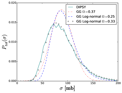
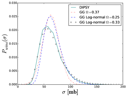
Figure 3: Fluctuations in the total (a) and inclusively wounded (b) cross section by

DIPSY

and the Glauber–Gribov model with different parametrisations of the cross section fluctuations.

It is clearly seen, that the high-$\sigma$ tails of the DIPSY  distributions are not reproduced by the functional form for $P_{\mathrm{tot}}$ in eq. (64). Since DIPSY  provides a picture of the fluctuations built upon a full dynamical model, it is reasonable to believe that the shape of the DIPSY  distributions are closer to reality than eq. (64). We therefore try a new parametrisation which makes it easier to obtain a large high-$\sigma$ tail, namely a log-normal distribution:

$$P_{tot}(\ln\sigma)=\frac{1}{\Omega\sqrt{2\pi}}\exp\left(-\,\frac{\ln^{2}(\sigma/\sigma_{0})}{2\Omega^{2}}\right).$$ (78)

The fit to the DIPSY cross sections with the log-normal distribution is also shown in table 1. The corresponding distributions are shown in figure 3 for two different width parameters, labeled $\Omega=0.25$ and $\Omega=0.33$. We see that the larger value matches the DIPSY  distribution perfectly, while the lower value is close to the GG curve below the maximum but has a higher tail for larger $\sigma$.

We note, however, that for technical reasons the diffractive cross section in DIPSY is calculated demanding a central rapidity gap, restricting the masses to $M_{X}^{2}\leq\sqrt{s}\cdot(1\,\mathrm{GeV})$. This implies that the fluctuations are somewhat underestimated. We therefore believe that the functional form is quite realistic, while the width is underestimated. Results obtained when tuning instead to the experimental cross sections are presented in the folloing subsection.

4.3.2 Comparison to data

We now repeat the same procedure as in the previous section, but with experimental results for the relevant cross sections. There is no experimental access to the distributions in cross section, but the integrated inclusive and semi-inclusive cross sections are measured, and we here use values from ref. [56], extrapolated to $\sqrt{s_{NN}}=5$ TeV:

$$\sigma_{\mathrm{tot}}=93.2\pm 2.3\text{~{}mb,~{}}\sigma_{\mathrm{el}}=23.2\pm 1.2\text{~{}mb~{}and~{}}\sigma_{w_{\mathrm{inc}}}=63.0\pm 1.8\text{~{}mb}.$$ (79)

Note that the diffractive cross sections here have been extrapolated into unmeasured $M_{X}$ regions to the full $0<M_{X}<\sqrt{S}$ interval. As mentioned above this was not done in for the DIPSY diffractive cross sections in section 4.3.1, where by construction a rapidity gap is required at mid rapidity. Hence we expect that the fluctuations for DIPSY are underestimated as compared to data. The parameter values obtained by minimising the $\chi^{2}$ are listed in table 2.

	$\Omega$	$\sigma_{0}$	$\lambda$
Original parametrisation	0.82	77.75	0.677
Log-normal parametrisation	0.43	85	0.677

Table 2: GG parameter values obtained by fit to inclusive and semi-inclusive cross-section from data.

In figure 4 we compare the fits of the two parametrisations of $P_{w_{\mathrm{inc}}}(\sigma)$ shown above. We see that the new parametrisation provides larger fluctuations in the high-$\sigma$ tail, as expected. It should be noted that both fits reproduce the experimental cross sections well within the experimental errors. For comparison we also show log-normal distribution $P_{w_{\mathrm{inc}}}(\sigma)$, when it’s width and mean are fitted to DIPSY  by eye (denoted $\Omega=0.33$), which is significantly more narrow.

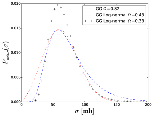
Figure 4: Fluctuations in the inclusively wounded cross section by the Glauber–Gribov model with two parametrisations of the cross section fluctuations, fitted to data.

We suspect that while the log-normal parametrisation probably gives a more realistic description of the high-$\sigma$ fluctuations in the GG formalism, it is far from the whole story. The GG results presented here are obtained assuming that all fluctuations are ascribed to fluctuations in projectile size, as described in section 4.2.4. In DIPSY , however, the cross section fluctuations arise from a combination of fluctuations in size and fluctuations in gluon density. We believe that updating the profile functions from simple disks or Gaussian distributions to more realistic ones, could provide a better handle on the parametrisations of the cross section from $\mathrm{pp}$ data, this will be investigated in a future publication. So far we have described a prescription which seems to both catch the necessary physics to calculate the inclusive wounded cross section, with all parameters being obtainable from $\mathrm{pp}$ data. We will now apply this to $\mathrm{p}A$ collisions.

4.4 Distributions of wounded nucleons

Using the considerations about fluctuations in the wounded cross section, we will now turn to generation of distributions of wounded nucleons. Normally, in inelastic, non-diffractive $\mathrm{p}A$ collisions, the number of wounded nucleons is always one plus the number of inelastic, non-diffractive $NN$ interactions. In the following we will make the distinction between diffractively and absorptively wounded nucleons. In order to avoid situations where the projectile should sometimes be counted twice as a wounded nucleon, we will solely talk about the number of wounded nucleons in the target, which we denote $N^{t}_{w}$. We note also that since the number of sub-collisions and the number of wounded nucleons are trivially connected, the question whether a specific observable scales better with wounded nucleons or with $NN$ sub-collisions, is much more relevant for nucleus–nucleus collisions.

4.4.1 Inclusively wounded nucleons

We will describe the nucleus’ transverse structure using a Woods–Saxon distribution in the GLISSANDO parameterisation [57, 58], where the density is given by:

$$\rho(r)=\frac{\rho_{0}(1+wr^{2}/R^{2})}{1+\exp((r-R)/a)},$$ (80)

where $R$ is the nuclear radius, $a$ is “skin width”, and $\rho_{0}$ is the central density. The parameter $w$ describes a possible non-constant density, but is zero for lead. The nucleons are generated with a hard core, which thus introduces short range correlations among the nucleons. As shown by Rybczynski and Broniowski [59], the correct two-particle correlation can be obtained if the nucleons are generated with a minimum distance equal to $2r_{\mathrm{core}}$. Using $r_{\mathrm{core}}=0.45$ fm and a skin width of $a=0.459$, the radius of the Lead nucleus becomes $R^{\mathrm{Pb}}=6.406$ according to the parameterisation in [58].

For each nucleus state we generate a random impact parameter wrt. the projectile proton and proceed to determine which nucleons will be wounded, following the previously outlined models.

In figure 5, we show the distribution in the number of inclusively wounded nucleons (using $\sigma_{w_{\mathrm{inc}}}^{\mathrm{\mathrm{pp}}}=63.0$ mb) for: a black disk model without any $\mathrm{pp}$ cross section fluctuations; GG with parameters fitted to data in section 4.3.2; GG with $P_{tot}(\sigma)$ given by eq. (78), also fitted to data; and the new simplified model outlined in section 4.1 (here called 2$\times 2$-disk) Fitting the latter to the cross sections in eq. (79) as well as to the double diffractive cross section $\sigma_{DD}=3.2$ mb, we obtain the parameters listed in table 3.

$r_{1}$	$r_{2}$	$\alpha$	$c$
0.15 fm	1.07 fm	0.97	0.42

Table 3: Table of parameters of the 2$\times 2$-disk model fitted to $\mathrm{pp}$ data.

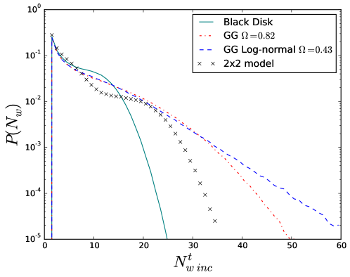
Figure 5: Distribution in the number of inclusively wounded nucleons, $N^{t}_{w_{\mathrm{inc}}}$, in $\mathrm{pPb}$ events at $\sqrt{s_{NN}}=5$ TeV, for a Glauber black disk, the GG model with two parametrisations of $P_{tot}(\sigma)$ and the 2$\times 2$-disk model. All models have been fitted to reproduce relevant measured (semi-) inclusive cross sections.

Looking at the individual distributions in figure 5, we see that all three inclusions of additional fluctuations in the cross section, significantly increases the tail of the distribution compared to the black disk. The 2$\times 2$-disk model has fewer fluctuations to very large $N_{w_{\mathrm{inc}}}^{t}$ numbers, and the dip in the distribution around $N^{t}_{w_{\mathrm{inc}}}=10$, also indicates that the fluctuations are too crude. The difference between GG with the original parametrisation and the log-normal distribution is visible in the tail above $N^{t}_{w_{\mathrm{inc}}}\approx 35$, as expected. One would therefore expect only an effect in the central events.

4.4.2 Distinguishing between absorptively and diffractively wounded nucleons

In our interpretation of the GG model in section 4.2.3, it can be used to calculate the sum of absorptively and diffractively wounded nucleons. In the Monte Carlo one would, however, like to have an impact parameter dependent recipe for each sub-collision to decide whether or not a target nucleon is diffractively or absorptively wounded, when hit by a projectile in a definite state $p$. This amounts to calculating the ratio of the absorptive to the inclusively wounded cross sections for a given sub-collision, and compare it to a random number

$$\frac{P_{w_{\mathrm{abs}},p}}{P_{w_{\mathrm{inc}},p}}=\frac{2\left\langle T_{p,t}(b)\right\rangle_{t}-\left\langle T_{p,t}(b)\right\rangle_{t}^{2}}{2\left\langle T_{p,t}(b)\right\rangle_{t}-\left\langle T^{2}_{p,t}(b)\right\rangle_{t}}.$$ (81)

For the 2$\times 2$-disk model this is done easily, as the above ratio reduces to:

$$\frac{P_{w_{\mathrm{abs}},p}}{P_{w_{\mathrm{inc}},p}}=\frac{2-\alpha}{2-\alpha\left\langle T^{2}_{p,t}(b)\right\rangle_{t}}.$$ (82)

The GG model on the other hand, implies averaging over target nucleon states, and provides thus no distinction. Instead we follow the 2$\times 2$-disk model to calculate the the conditional probability to be diffractively wounded, if a nucleon is already inclusively wounded in the GG model. This is:

$$P(\mathrm{diff}|w_{\mathrm{inc}})=\Theta\left(\sqrt{\sigma_{GG}/\pi}-(r_{1}-r_{2})-b\right)\frac{2-\alpha}{2-\alpha c},$$ (83)

where the first term is a requirement that the two nucleons are separated by an amount such that a fluctuation in size is necessary to be wounded. In figure 6 we show distributions of $N^{t}_{w_{\mathrm{abs}}}$ for the 2$\times 2$-disk model and for the corrected GG model, using both parametrisations of $P(\sigma)$.

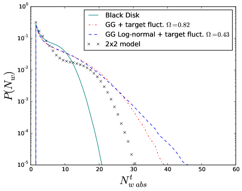
Figure 6: Distribution in the number of absorptively wounded nucleons, $N^{t}_{w_{\mathrm{abs}}}$, in $\mathrm{pPb}$ events at $\sqrt{s_{NN}}=5$ TeV, for a Glauber black disk, the GG model with two parametrisation of $P(\sigma)$, corrected using the 2$\times 2$-disk model, along with the 2$\times 2$-disk model itself. All models have been fitted to reproduce relevant measured (semi-) inclusive cross sections.

5 Modelling final states in $\mathrm{p}A$ collisions

In this section we will take the knowledge about distributions of wounded nucleons and investigate the consequences for final states in $\mathrm{p}A$ collisions. We will discuss a few views on modelling particle production in such collisions, all assuming that a full final state of a $\mathrm{p}A$ collision can be adequately modelled by stacking $\mathrm{pp}$ events on top of each other, here modelled using P YTHIA 8. Following the introduction of the models, we will compare to data, both multiplicity as function of centrality, and inclusive $p_{\perp}$ spectra. Finally we will give an estimate of the theoretical uncertainties present at this early stage of the model.

5.1 Generating final states with P YTHIA 8

The general methodology for generating final states, which will be pursued here, will have the following ingredients:

• For each collision, a Glauber calculation is performed as outlined in section 4.4, setting up the nuclear geometry.

• The total number of inclusively wounded target nucleons is calculated, as well as the number of absorptively wounded targets, if the two differ in the considered approach.

• Sub-collisions are generated as $\mathrm{pp}$ collisions, according to two separate approaches, which will be outlined in the following.

• Each sub-collision is treated separately in terms of colour reconnection and hadronisation. Efforts to include cross talk between sub-collisions will be the subject of a future publication.

Cross talk between sub-collisions is, however, included in one respect by accounting for energy-momentum conservation in all approaches. As before, we will concentrate on $\mathrm{pPb}$ collisions at $\sqrt{s_{NN}}=5$ TeV. The methodology is, however, not limited to this, and generalisation to $AA$ collisions will be the subject of a future publication.

5.2 Wounded nucleons and multi-parton interactions

In ref. [25] Białas et al. noticed that the central particle density in $\mathrm{p}A$ collisions scales approximately with the number of ”wounded” or ”participating” nucleons, $dN^{(\mathrm{p}A)}/d\eta\approx(N_{wounded}/2)\,dN^{(\mathrm{pp})}/d\eta$. The projectile proton was here included as one of the wounded nucleons, and the distribution in rapidity could be described if each wounded target nucleon gives a contribution proportional to $(\eta-\eta_{t})/(\eta_{p}-\eta_{t})$ where $\eta_{t,p}$ are the rapidities of the target and projectile respectively. The wounded projectile proton gives a similar contribution with $p$ exchanged for $t$.

The wounded nucleon model worked well for minimum bias events and low $p_{\perp}$ particles, while high $p_{\perp}$ particles scale better with the number of $NN$ collisions, which can be understood if the high-$p_{\perp}$ particles originate from independent partonic subcollisions. (See e.g. ref. [60].) A model with this feature, called G-Pythia, has been used in analyses by ALICE [17].

These results can be given a heuristic interpretation in terms of the Landau-Pomeranchuk formation time. The formation time for a hadron is, in a frame where $p_{L}=0$:

$$\tau\geq\frac{1}{\sqrt{p_{\perp}^{2}+m^{2}}}.$$ (84)

This implies that a produced pion will resolve the nucleus at a length scale given roughly by $1/p_{\perp}$. For $p_{\perp}<1$ GeV the resolution scale is larger than that of the individual nuclei, while for $p_{\perp}$ larger than $\sim 1$ GeV, constituents of individual nucleons can be resolved.

Below we will compare two models, generated with the help of P YTHIA 8. The model denoted ”Absorptive” is similar to G-Pythia. Here each $NN$ subcollision is treated as a $\mathrm{pp}$ collision. The second model, explained in the next subsection, is called FritiofP8 and is more similar to the wounded nucleon model. We note that the models should not be compared on equal footing. From the above arguments, the ”Absorptive” model is expected to describe the high-$p_{\perp}$ part of the spectrum better, while FritiofP8, being similar to the wounded nucleon model, is expected to describe the low-$p_{\perp}$ part, and thus also the total multiplicity, best.

Technically, the subcollisions are in both models generated with P YTHIA 8. This means that for each sub-collision, multiple partonic interactions are created in decreasing order of $p_{\perp}$ with the probability:

$$\frac{d\mathcal{P}}{dp_{\perp i}}=\frac{1}{\sigma_{\mathrm{abs}}}\frac{d\sigma_{2\rightarrow 2}}{dp_{\perp i}}\exp\left[-\int_{p_{\perp i}}^{p_{\perp}i-1}\frac{1}{\sigma_{\mathrm{abs}}}\frac{d\sigma_{2\rightarrow 2}}{dp_{\perp}^{\prime}}dp_{\perp}^{\prime}\right],$$ (85)

starting from a maximum scale related to the impact parameter of the sub-collision. The cross section is obtained by treating everything as perturbative QCD $2\rightarrow 2$ scatterings, but since the cross section diverges at low $p_{\perp}$, it is regulated at low $p_{\perp}$ using:

$$\frac{d\sigma_{2\rightarrow 2}}{dp_{\perp}^{2}}\propto\frac{\alpha^{2}_{s}(p^{2}_{\perp})}{p^{4}_{\perp}}\rightarrow\frac{\alpha^{2}_{s}(p^{2}_{\perp}+p^{2}_{\perp 0})}{(p^{2}_{\perp}+p^{2}_{\perp 0})^{2}}.$$ (86)

Here $p_{\perp 0}$ is a tunable parameter.

Aside from momentum conservation, P YTHIA 8 also rescales the PDF every time a quark has been used in an MPI. When using this MPI model for generating $\mathrm{p}A$ collisions we maintain momentum conservation, but do not maintain the rescaling of the PDF between separate $NN$ collisions.

5.3 The revived Fritiof model

A very different approach was used in the Fritiof model [23]. Where the P YTHIA 8 MPI model assumes everything can be described by perturbative scatterings, Fritiof imposed a soft model for everything, specifically limiting it’s range of validity to low-$p_{\perp}$ processes.

In the Fritiof model it is assumed that a soft min-bias interaction causes a momentum exchange, which in light-cone variables has the form

$$P(Q_{+},Q_{-})\propto\frac{dQ_{+}}{Q_{+}}\frac{dQ_{-}}{Q_{-}}.$$ (87)

This produces two excited states assumed to decay like strings stretching the rapidity range between the initial beam rapidities and a point distributed evenly within the kinematically allowed region The result is approximately reproducing the original wounded nucleon model [25], but it is in the Fritiof model also assumed that a secondary encounter with another nucleon will increase the excitation, thus leading to a logarithmic scale breaking.

In ref. [61] it was suggested to extend the Fritiof model to include the possibility for a hard scattering and associated bremsstrahlung when the energy is high enough. At LHC collision energies, the necessity for including the possibility for at least one such interaction is apparent.

Figure 7: Cartoon in rapidity–impact-parameter space, showing the evolution of exchanged gluons between a projectile proton and a number of wounded nucleons in the target nucleus. Nucleons $\nu_{1},\ldots,\nu_{4}$ are wounded absorptively, while $\nu_{5}$ is wounded diffractively. $\nu_{4}$ is considered to be the primary wounded nucleon.

In figure 7 we show a schematic picture of a projectile proton wounding a number of nucleons. The picture is strongly oversimplified, showing only the main gluon propagators, i.e. no initial/final-state radiation (ISR/FSR) or multi-parton interactions (MPI) in the individual sub-collision. Nucleons $\nu_{1},\ldots\nu_{4}$ are wounded absorptively with $\nu_{4}$ being the hardest or ”primary” wounded nucleon, which contributes to the hadronic multiplicity the full rapidity region. The other absorptively wounded nucleons, $\nu_{1}\ldots\nu_{3}$, contributes only to the parts of the rapidity range in the nucleus direction. As indicated by the exchanged Pomeron, $I\!\!P$, $\nu_{5}$ is only diffractively excited, and will also only contribute in the nucleus direction.

Figure 8: Pomeron diagrams with cuts indicated for (a) single diffractive excitation in proton–proton and (b) doubly absorptive proton–deuteron scattering.

Thinking in terms of cut Pomeron diagrams à la AGK [62] we show in figure 8 the similarity between the diagram describing diffractive excitation in proton–proton scattering and a fully absorptive proton–deuteron scattering. It is not far fetched to assume that the triple-Pomeron vertex in both cases are distributed in approximately the same way in rapidity, i.e., that the gap size in the single diffractive excitation in $\mathrm{pp}$ would be distributed in the same way as the the size of the region of rapidity populated by hadrons from both wounded nucleons in a $\mathrm{pd}$ collision.

As discussed in section 3.3 the distribution in diffractive masses indicates a fairly flat distribution in rapidity of the triple-Pomeron vertex as $\epsilon$ is close to zero. We will therefore assume as a first approximation, that the secondary absorptive collisions in a $\mathrm{p}A$ collision can be approximated by single diffractive collisions.

Treating secondary absorptive collisions as single diffractive excitation has an additional added benefit. In the P YTHIA 8 implementation, one can model high mass soft excitation using a perturbative approach where the exited proton can undergo multiple partonic interactions, as in eq. (85), and ISR is included. It is thus possible to treat absorptively wounded nucleons differently, depending on whether the mass of the excited system is larger or smaller than a pre-set threshold mass scale.

Finally, in figure 7, we also have $\nu_{5}$, which is an standard diffractively excited nucleon, and will be modelled as such.

5.4 Comparison to data

We now compare the two methods for particle production, which were introduced above. Stacking absorptive events on top of each other is labelled “Absorptive”, we use a black disk Glauber model with $\sigma_{abs}=67.9$ mb to calculate the number of absorptive sub-collisions event by event. The model including both diffractive excitation and the Fritiof-inspired absorptive sub-collisions is labelled “FritiofP8”. To calculate the amount of wounded nucleons we use the modified GG model with cross section fluctuations described by the log-normal distribution in eq. (78) and including the modifications introduced in section 4.2.4, as well as distinguishing between absorptive and diffractive events using the 2$\times 2$-disk modification, introduced in section 4.4.2. All parameters are fitted to $\mathrm{pp}$ data.

5.4.1 Centrality estimation and multiplicity

The primary observable we wish to discuss, is the charged particle pseudo-rapidity distribution at different centralities, as measured by ATLAS [16]. When comparing Monte Carlo predictions to data in $\mathrm{pp}$, the work flow has matured greatly over the past years, with the advent of automated frameworks for performing such tasks, such as Rivet [63]. In this framework, equal treatment of theory and unfolded data is ensured by publishing measurements along with an implementation of the analysis. This is not yet tradition in the heavy ion community, and the data comparisons shown here, is the result of our own Rivet implementation on the analysis, based on the paper, with data obtained from HepData [64].

In the experimental analysis by ATLAS, event centrality is calculated by taking fractiles of the distribution in $\sum E_{\perp}$ of charged particles in the interval $3.1<\eta<4.9$. For this particular observable, unfolded data has not been published, but we will still compare theoretical curves for the two previously outlined particle production models. In figure 9 we show the model stacking $N^{t}_{w_{\mathrm{abs}}}$ absorptive events spanning the whole rapidity region (denoted “Absorptive”) reaches a much higher $\sum E_{\perp}$ than the Fritiof inspired model (denoted “FritiofP8”) With one absorptive event spanning the whole rapidity region, $N^{t}_{w_{\mathrm{abs}}}-1$ absorptive events modelled as diffractive excitation, and $N^{t}_{w_{\mathrm{inc}}}-N^{t}_{w_{\mathrm{abs}}}$ events from diffractive excitation. We note that the “FritiofP8” results agree almost perfectly with the data from Atlas, while the Absorptive model reaches significantly higher $\sum E_{\perp}$ values.

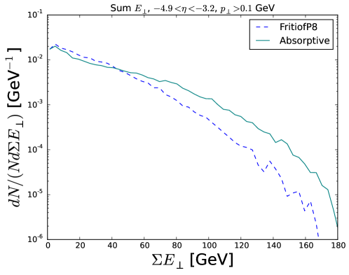
Figure 9: Distribution in $\sum E_{\perp}$ for a sum of full absorptive events and the new FritiofP8 model, for $\mathrm{pPb}$ collisions at $\sqrt{s_{NN}}=5$ TeV.

In figure 10 we show pseudorapidity distributions for different centralities, where we have used the same cuts as ATLAS, but reconstructed fractiles from our own distribution.

(a)

(b)

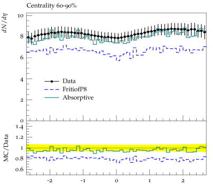
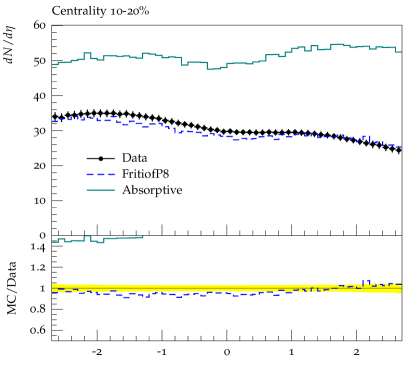
(c)

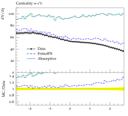
Figure 10: Pseudo-rapidity distribution of charged particle multiplicity for centralities $60-90\%$ (a), $20-30\%$ (b), and $0-1\%$ (c), compared to “Absorptive” and “FritiofP8” particle production models.

We see that while both models describe the peripheral events reasonably well (which is expected), the new FritiofP8 model based on diffractive excitation does a much better job describing both average multiplicity and the forward–backward asymmetry, as expected.

5.4.2 Inclusive transverse momentum

We now compare to centrality-inclusive charged particle $p_{\perp}$ spectra in different ranges of $\eta$ as measured by CMS [65]. In figure 11a we show the transverse momentum distribution for $-1.0<\eta<1.0$. We see that the FritiofP8 model performs well at low $p_{\perp}$, while Absorptive performs well at high $p_{\perp}$, as expected.

(a)

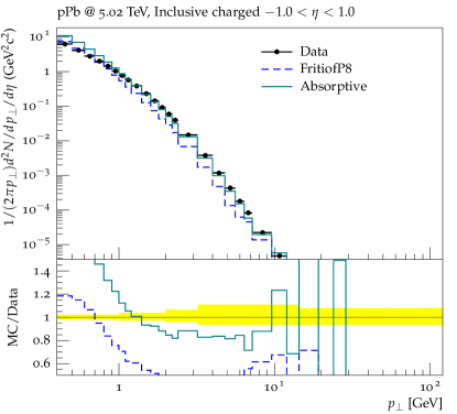
(b)

(c)

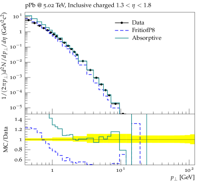
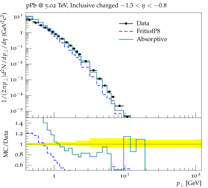
Figure 11: Distribution in $p_{\perp}$, centrality inclusive, for charged particles in (a) the central region, $-1.0<\eta<1.0$; (b) the proton direction, $1.3<\eta<1.8$; and (c) the nucleus direction $-1.3<\eta<0.8$.

The same picture is seen when going to large negative $\eta$ (figure 11c), but performance of the FritiofP8 model improves slightly when going to large positive $\eta$ shown in figure 11b for $1.3<\eta<1.8$ (the proton side). The ”absorptive” model performs as before, but it is rather surprising that the FritiofP8 model performs poorly at high $p_{\perp}$ here. One explanation could be that the parton distribution function used for for secondary absorptive events is a Pomeron PDF and not a proton PDF, due to the fact that secondary absorptive events are modelled as single diffractive events. This is also a possible explanation for the poor performance at high $p_{\perp}$ in figure 11a and figure 11c.

5.5 Uncertainties

The method presented here for generating final states in $\mathrm{p}A$ is interesting, as it gives qualitatively correct description of the multiplicity in both the proton and the nucleus direction. It is still mostly a proof-of-principle since, as we will demonstrate here, using the P YTHIA 8 default settings introduces several hidden assumptions. We will discuss these assumptions by giving a rough estimate of the uncertainty associated with each of them. That uncertainty will decrease, or vanish entirely, when the assumptions are dealt with more carefully, one by one, which will be done in one or more future publications.

5.5.1 PDFs and MPI activity

In the previous section we described how the secondary absorptive sub-collisions are approximated as single diffractive excitation events. The perturbative handling of single diffractive events at high masses in P YTHIA 8 relies on a factorised Pomeron approach, where the diffractive state is modelled by a Pomeron–proton collision, including MPI, and we will study two important uncertainties here.

• The Pomeron PDFs used in the MPI machinery are not really appropriate in our model of the secondary absorptive sub-collisions, since it is still really the parton density in the proton which should drive the MPI. To see possible effects, we have tried to make the Pomeron more proton-like, by modifying the PDF used in P YTHIA 8 to have much more small-$x$ gluons. This will increase MPI activity.

• Another way of modifying the MPI activity is to change the Pomeron–proton cross section used in P YTHIA 8. This is not a physical cross section, but rather a free parameter in the program which only affects MPI activity, and is adjusted to fit data. The default value of this parameter is $10$ mb. We here increase it to it’s maximal allowed value, $40$ mb, to better reflect a $pp$ absorptive cross section.

In figure 12 we show the pseudo-rapidity distribution of charged particles for the highest centrality bin. The two variations above are labelled “PDF” and “MPI” respectively while FritiofP8 is the same as before.

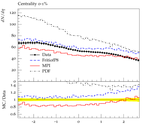
Figure 12: Pseudo-rapidity distribution of charged particle multiplicity for centrality $0-1\%$ compared to three different ways of estimating the number of MPIs, giving an estimate of the method uncertainty.

In total, the envelope of the three lines gives what we believe to be a reasonable, albeit conservative, estimate of the uncertainty so far associated with the approximations regarding the parton densities and the amount of MPIs.

5.5.2 GG uncertainty

In section 4.3.1 we described how the Glauber–Gribov cross section fluctuations could be parameterised with a log-normal distribution. This new parameterisation was used in all the previous data comparison plots, here we show how the traditional parameterisation (also fitted to $\mathrm{pp}$ data) compared to the new one. Since distributions of wounded nucleons for the two models differs most in the tail, we are most sensitive in central collisions, In figure 13 we show the uncertainty in central particle production arising from changing the parametrisation of cross section fluctuations. We see that the uncertainty covers data well, but is smaller than the uncertainties in the handling of secondary absorptive events above.

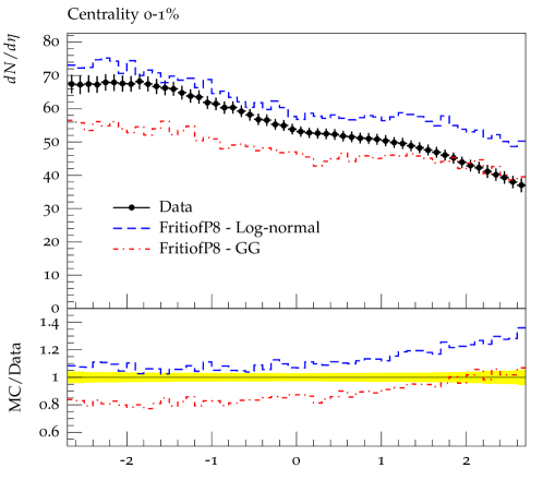
Figure 13: Pseudo-rapidity distribution of charged particle multiplicity for centrality $0-1\%$ compared to two parameterisations for the GG model.

6 Conclusions and outlook

Collisions of heavy nuclei with protons or each other, are often understood in terms of their deviation from minimum bias $\mathrm{pp}$ collisions, which after many years of work on models for multiple partonic interactions, are fairly well understood. The extrapolation from $\mathrm{pp}$ to $\mathrm{p}A$ or $AA$, which is usually based on Glauber models, is therefore a crucial step toward understanding the deviations, and thus crucial for understanding how and if a de-confined plasma of quarks and gluons are created in heavy ion collisions, and what kind of impact it has on final state observables. In this article we have discussed Glauber models, their extensions including fluctuations and the impact these extensions on the number of wounded nucleons, followed by a possible way of using that knowledge to generate full, exclusive final states as a sum of $\mathrm{pp}$ collisions. We will conclude on these two parts separately, followed by an outlook primarily focused on extending the model for full final states, to also include microscopic models for collective effects.

6.1 Fluctuations in the Glauber formalism

Following Good and Walker, we have discussed diffractive excitation as a manifestation of fluctuations in the substructure of the nucleons. As a result of this discussion we identified the inclusively wounded cross section to be the relevant $\mathrm{pp}$ cross section for calculations of the number of wounded nucleons. The wounded cross section has contributions from absorptive processes plus diffractively excited target nucleons, in brief form we have for the semi-inclusive $\mathrm{pp}$ cross sections:

$$\sigma_{w_{\mathrm{inc}}}=\sigma_{\mathrm{abs}}+\sigma_{\mathrm{DD}}+\sigma_{\mathrm{Dt}}=\sigma_{\mathrm{tot}}-\sigma_{\mathrm{el}}-\sigma_{\mathrm{Dp}}.$$ (88)

We have discussed the developments in calculating the number distribution of inclusively wounded nucleons in the so-called Glauber–Gribov approach by Strikman and co-workers. By comparing distributions of the cross section to ones calculated with the DIPSY model and measurements, we find that the parametrisation of the cross section suggested in the Glauber–Gribov approach does not fully include all fluctuations necessary to describe the ones in DIPSY .

The simplest Glauber calculations using a fixed black disk, can clearly not describe any fluctuations, and we want to emphasize that just setting $\sigma_{NN}=\sigma_{w_{\mathrm{inc}}}$ in such a calculation, is not enough if one wants to calculate the contribution from the wounded nucleons to a centrality defining observable.

We have shown that a Glauber–Gribov calculation with a black disk fluctuating in size, can be used to predict the distribution of inclusively wounded nucleons, if the fluctuating black disk is attributed to fluctuations in the projectile, while averaging over fluctuations in the target nucleon. However, if one wants to separate absorptively wounded nucleons from diffractively wounded ones, it is necessary to also consider fluctuations in the individual target nucleons.

We have suggested a new functional form for the fluctuations in the $\mathrm{pp}$ interaction, with a higher tail to a larger cross section. Instead of the parametrization introduced by Strikman et al., and used in several experimental analyses, we suggest a log-normal distribution, which is believed to give a somewhat better description of the inclusive distribution, though not necessarily a more realistic picture of the cross section fluctuations. We have also included fluctuations in the target nucleons by introducing a crude Glauber-like model, where the radii of the projectile and target are allowed to fluctuate independently between two values. The model includes four parameters, and can be fitted to describe four independent semi-inclusive $\mathrm{pp}$ cross sections, including the inclusive wounded one. By using this model to include projectile fluctuations in the Glauber–Gribov approach, we separate the inclusively wounded nucleon into absorptively and diffractively wounded ones.

The parametrisations and toy-models studied are built on the assumption that distributions of wounded nucleons can be described solely by fluctuations in the proton size; projectile size for the inclusive distributions, and target nucleon size for distinguishing between absorptively and diffractively wounded nucleons. Thinking about the dynamics of more involved calculations, like the DIPSY model used in this paper, it is clear that size fluctuations cannot account for all the relevant physics. In the DIPSY model, fluctuations in cross section will also arise when e.g. a small projectile is very dense, and therefore gives rise to a larger cross section. Similarly, a large projectile can be dilute, giving rise to a smaller cross section. In the language of this article, such effects would need to be accounted for by a fluctuating, $b$-dependent opacity, resulting in a profile function which would go beyond the simple Gaussian, grey -or black disks, but still not be as calculationally involved as the full, dynamical models. This will be the subject of a future publication.

6.2 Full final states

We have given a proof-of-principle for an approach to model exclusive final states in $\mathrm{p}A$ collisions as a sum of several $\mathrm{pp}$ collisions. The approach uses P YTHIA 8 to calculate the hardest absorptive sub-collision as a normal non-diffractive $\mathrm{pp}$ collision, while the subsequent absorptive collisions are modelled as single diffractive events. This was inspired by the old Fritiof model, which is valid at lower energies, but adds another dimension, as high-mass single diffractive exchanges can now be treated perturbatively and allows for multiple parton–parton scatterings.

We have shown that this approach, in a quite crude implementation, is able to give a reasonable description of some recently published final-state measurements of $\mathrm{pPb}$ collisions at the LHC, but the uncertainties in our approach are quite large. In future studies we will try to eliminate these uncertainties, in the hope to get a theoretically well motivated and more accurate description of data.

To do this it is helpful to have data published in a usable form for comparison with event generators. The LHC $\mathrm{pp}$ community has come a long way in this respect by publishing many of their results in the form of Rivet routines. In this way the measurements are presented in a clearly reproducible form, including all relevant kinematical cuts and unfolding of detector effects but free from dependence of theoretical models. In order to allow for the development of better event generators for heavy ion collisions, it is imperative that the experimental heavy ion community adapts a similar way of presenting their results.

6.3 Outlook: modelling collective effects

In both the theoretical and experimental communities around heavy ion collisions, much attention is given to observables thought to convey information about a possible plasma state created in the collision. A direct application of the work presented in this article, is to use the final state extrapolation as a baseline for calculations of collective effects using microscopic, QCD based models. In the $\mathrm{pp}$ community, much attention have been given to models of final state interactions including colour reconnections, rope hadronisation and junction formation [67, 68, 69]. These models have, in $\mathrm{pp}$  been shown to reproduce: the enhancement of strange hadrons to non-strange hadrons in dense environments [70]; flow-like effects in hadron ratios as function of $p_{\perp}$; and preliminary studies have shown that interactions between strings can produce a ridge [71].

To implement such models in a framework like the one presented here, a necessary component is a good understanding of the sub-collisions in transverse space. Such a picture is not included in e.g. the P YTHIA 8 MPI model, and must therefore be added a posteriori. Guidance can then be had from the DIPSY model, which includes detailed information about the transverse space structure, but does not produce final states describing data as well as P YTHIA 8.

Finally, the final state model introduced here should be developed further to model fully exclusive hadronic final states also in $AA$ collisions. Since every projectile here also becomes a target, we suspect that the model cannot be transferred one-to-one, but that some modifications may be needed. Here modelling collective effects using microscopic models is also highly desirable.

References

- [1] A. Bzdak and V. Skokov, Phys. Rev. Lett. 111 (2013) 182301, arXiv:1307.6168 [hep-ph].
- [2] L. McLerran and M. Praszalowicz, arXiv:1507.05976 [hep-ph].
- [3] R. J. Glauber, Phys. Rev. 100 (1955) 242–248.
- [4] M. L. Miller, K. Reygers, S. J. Sanders, and P. Steinberg, Ann.Rev.Nucl.Part.Sci. 57 (2007) 205–243, arXiv:nucl-ex/0701025 [nucl-ex].
- [5] CDF Collaboration, F. Abe et al., Phys. Rev. D50 (1994) 5535–5549.
- [6] ATLAS Collaboration, G. Aad et al., Eur. Phys. J. C72 (2012) 1926, arXiv:1201.2808 [hep-ex].
- [7] CMS Collaboration, V. Khachatryan et al., Phys. Rev. D92 (2015) no.~1, 012003, arXiv:1503.08689 [hep-ex].
- [8] V. N. Gribov, Sov. Phys. JETP 29 (1969) 483–487. [Zh. Eksp. Teor. Fiz.56,892(1969)].
- [9] G. Gustafson, L. Lönnblad, A. Ster, and T. Csörgő, JHEP 10 (2015) 022, arXiv:1506.09095 [hep-ph].
- [10] H. Heiselberg, G. Baym, B. Blaettel, L. L. Frankfurt, and M. Strikman, Phys. Rev. Lett. 67 (1991) 2946–2949.
- [11] B. Blaettel, G. Baym, L. L. Frankfurt, H. Heiselberg, and M. Strikman, Phys. Rev. D47 (1993) 2761–2772.
- [12] M. Alvioli and M. Strikman, Phys. Lett. B722 (2013) 347–354, arXiv:1301.0728 [hep-ph].
- [13] M. Alvioli, L. Frankfurt, V. Guzey, and M. Strikman, Phys. Rev. C90 (2014) 034914, arXiv:1402.2868 [hep-ph].
- [14] M. Alvioli, B. A. Cole, L. Frankfurt, D. V. Perepelitsa, and M. Strikman, arXiv:1409.7381 [hep-ph].
- [15] M. L. Good and W. D. Walker, Phys. Rev. 120 (1960) 1857–1860.
- [16] ATLAS Collaboration, G. Aad et al., arXiv:1508.00848 [hep-ex].
- [17] ALICE Collaboration, J. Adam et al., Phys. Rev. C91 (2015) no.~6, 064905, arXiv:1412.6828 [nucl-ex].
- [18] E. Avsar, G. Gustafson, and L. Lönnblad, JHEP 07 (2005) 062, arXiv:hep-ph/0503181 [hep-ph].
- [19] E. Avsar, G. Gustafson, and L. Lönnblad, JHEP 01 (2007) 012, arXiv:hep-ph/0610157 [hep-ph].
- [20] C. Flensburg, G. Gustafson, and L. Lönnblad, JHEP 1108 (2011) 103, arXiv:1103.4321 [hep-ph].
- [21] A. H. Mueller, Nucl. Phys. B415 (1994) 373–385.
- [22] A. H. Mueller and B. Patel, Nucl. Phys. B425 (1994) 471–488, arXiv:hep-ph/9403256 [hep-ph].
- [23] B. Andersson, G. Gustafson, and B. Nilsson-Almqvist, Nucl. Phys. B281 (1987) 289.
- [24] H. Pi, Comput. Phys. Commun. 71 (1992) 173–192.
- [25] A. Białas, M. Bleszynski, and W. Czyz, Nucl. Phys. B111 (1976) 461.
- [26] A. Bialas, J. Phys. G35 (2008) 044053.
- [27] PHOBOS Collaboration, B. B. Back et al., Phys. Rev. C72 (2005) 031901, arXiv:nucl-ex/0409021 [nucl-ex].
- [28] PHENIX Collaboration, A. Adare et al., Phys. Rev. C90 (2014) no.~3, 034902, arXiv:1310.4793 [nucl-ex].
- [29] ALICE Collaboration, B. Abelev et al., Phys. Rev. Lett. 110 (2013) no.~3, 032301, arXiv:1210.3615 [nucl-ex].
- [30] T. Sjöstrand and M. van Zijl, Phys. Rev. D36 (1987) 2019.
- [31] T. Sjöstrand, S. Ask, J. R. Christiansen, R. Corke, N. Desai, et al., arXiv:1410.3012 [hep-ph].
- [32] M. Bahr et al., Eur. Phys. J. C58 (2008) 639–707, arXiv:0803.0883 [hep-ph].
- [33] T. Gleisberg, S. Hoeche, F. Krauss, M. Schonherr, S. Schumann, F. Siegert, and J. Winter, JHEP 02 (2009) 007, arXiv:0811.4622 [hep-ph].
- [34] L. D. McLerran and R. Venugopalan, Phys.Rev. D49 (1994) 2233–2241, arXiv:hep-ph/9309289 [hep-ph].
- [35] C. Flensburg, G. Gustafson, and L. Lönnblad, Eur. Phys. J. C60 (2009) 233–247, arXiv:0807.0325 [hep-ph].
- [36] C. Flensburg and G. Gustafson, JHEP 1010 (2010) 014, arXiv:1004.5502 [hep-ph].
- [37] A. H. Mueller, Phys. Rev. D2 (1970) 2963–2968.
- [38] E. Gotsman, E. Levin, and U. Maor, Int. J. Mod. Phys. A30 (2015) no.~08, 1542005, arXiv:1403.4531 [hep-ph].
- [39] V. A. Khoze, A. D. Martin, and M. G. Ryskin, Int. J. Mod. Phys. A30 (2015) no.~08, 1542004, arXiv:1402.2778 [hep-ph].
- [40] S. Ostapchenko, Phys.Rev. D83 (2011) 014018, arXiv:1010.1869 [hep-ph].
- [41] H. I. Miettinen and J. Pumplin, Phys. Rev. D18 (1978) 1696.
- [42] Y. Hatta, E. Iancu, C. Marquet, G. Soyez, and D. Triantafyllopoulos, Nucl.Phys. A773 (2006) 95–155, arXiv:hep-ph/0601150 [hep-ph].
- [43] E. Avsar, G. Gustafson, and L. Lönnblad, JHEP 12 (2007) 012, arXiv:0709.1368 [hep-ph].
- [44] G. Gustafson, arXiv:1206.1733 [hep-ph].
- [45] C. Flensburg, G. Gustafson, and L. Lönnblad, JHEP 1212 (2012) 115, arXiv:1210.2407 [hep-ph].
- [46] M. Alvioli, H. J. Drescher, and M. Strikman, Phys. Lett. B680 (2009) 225–230, arXiv:0905.2670 [nucl-th].
- [47] M. Alvioli, H. Holopainen, K. J. Eskola, and M. Strikman, Phys. Rev. C85 (2012) 034902, arXiv:1112.5306 [hep-ph].
- [48] B. Alver, M. Baker, C. Loizides, and P. Steinberg, arXiv:0805.4411 [nucl-ex].
- [49] C. Loizides, J. Nagle, and P. Steinberg, SoftwareX 1-2 (2015) 13–18, arXiv:1408.2549 [nucl-ex].
- [50] L.-K. Ding and E. Stenlund, Comput. Phys. Commun. 59 (1990) 313–318.
- [51] G. Antchev et al., Europhys. Lett. 96 (2011) 21002, arXiv:1110.1395 [hep-ex].
- [52] TOTEM Collaboration, G. Antchev et al., Europhys. Lett. 101 (2013) 21002.
- [53] TOTEM Collaboration, G. Antchev et al., Europhys. Lett. 95 (2011) 41001, arXiv:1110.1385 [hep-ex].
- [54] ALICE Collaboration, B. Abelev et al., Eur. Phys. J. C73 (2013) no.~6, 2456, arXiv:1208.4968 [hep-ex].
- [55] UA4 Collaboration, D. Bernard et al., Phys. Lett. B186 (1987) 227–232.
- [56] P. Lipari and M. Lusignoli, Eur. Phys. J. C73 (2013) no.~11, 2630, arXiv:1305.7216 [hep-ph].
- [57] W. Broniowski, M. Rybczynski, and P. Bozek, Comput. Phys. Commun. 180 (2009) 69–83, arXiv:0710.5731 [nucl-th].
- [58] M. Rybczynski, G. Stefanek, W. Broniowski, and P. Bozek, Comput. Phys. Commun. 185 (2014) 1759–1772, arXiv:1310.5475 [nucl-th].
- [59] M. Rybczynski and W. Broniowski, arXiv:1012.5607 [nucl-th].
- [60] A. Białas, Journal of Physics G: Nuclear and Particle Physics 35 (2008) no. 4, 044053.
- [61] B. Andersson, G. Gustafson, and H. Pi, Z. Phys. C57 (1993) 485–494.
- [62] V. Abramovsky, V. Gribov, and O. Kancheli, Yad.Fiz. 18 (1973) 595–616.
- [63] A. Buckley et al., arXiv:1003.0694 [hep-ph].
- [64] A. Buckley, W. J. Stirling, M. R. Whalley, J. M. Butterworth, J. Monk, E. Nurse, and B. Waugh, , in 15th International Conference on Computing in High Energy and Nuclear Physics (CHEP 2006) Mumbai, Maharashtra, India, February 13-17, 2006. 2006. arXiv:hep-ph/0605048 [hep-ph].
- [65] CMS Collaboration, V. Khachatryan et al., Eur. Phys. J. C75 (2015) no.~5, 237, arXiv:1502.05387 [nucl-ex].
- [66] H1 Collaboration, A. Aktas et al., Eur. Phys. J. C48 (2006) 715–748, arXiv:hep-ex/0606004 [hep-ex].
- [67] C. Bierlich, G. Gustafson, L. Lönnblad, and A. Tarasov, JHEP 03 (2015) 148, arXiv:1412.6259 [hep-ph].
- [68] C. Bierlich and J. R. Christiansen, Phys. Rev. D92 (2015) no.~9, 094010, arXiv:1507.02091 [hep-ph].
- [69] J. R. Christiansen and P. Z. Skands, JHEP 08 (2015) 003, arXiv:1505.01681 [hep-ph].
- [70] ALICE Collaboration, J. Adam et al., arXiv:1606.07424 [nucl-ex].
- [71] I. Altsybeev, AIP Conf. Proc. 1701 (2016) 100002, arXiv:1502.03608 [hep-ph].