Synchrotron contribution to photon emission from quark-gluon plasma

Abstract

We study the influence of the magnetic field on the photon emission from the quark-gluon plasma created in $AA$ collisions. We find that even for very optimistic assumption on the magnitude of the magnetic field for noncentral $AA$ collisions the effect of magnetic field is very small.

I Introduction

Experimental study of photon spectra in the low and intermediate $k_{T}$ region in $AA$ collisions can provide vital information on the parameters of the produced quark-gluon plasma (QGP) Shuryak . It is widely believed that the observed in $AA$ collisions at RHIC PHENIX_ph1 ; PHENIX_ph_v2 ; PHENIX_ph_PR and LHC ALICE_ph excess of the photon yield (above the photons from hadron decays and from the hard perturbative mechanism) at $k_{T}\mathrel{\hbox to0.0pt{\lower 4.0pt\hbox{\hskip 1.0pt$\sim$}\hss}\raise 1.0pt\hbox{$<$}}3-4$ GeV is related to photon emission from the QGP. It is surprising that the thermal photons exhibit a significant azimuthal asymmetry $v_{2}$ (“elliptic flow”) comparable to that for hadrons. It is difficult to reconcile with the expectation that the thermal photons should be mostly radiated from the hottest initial stage of the QGP where the flow effects should be small (it is usually called “the direct photon puzzle”).

It was suggested by Tuchin T1 that the azimuthal anisotropy of the direct photons may be due to synchrotron mechanism of the photon emission in a strong transverse (to the reaction plane) magnetic field in the noncentral $AA$ collisions. The synchrotron contribution obtained in T1 can explain a significant fraction of the photon yield in the central rapidity region at $k_{T}\sim 1-3$ GeV. However, the calculations performed in T1 are of a qualitative nature. In particular in T1 it was ignored the fact that multiple scattering of quarks, which they undergo in the thermal bath, will suppress the synchrotron emission (because of reduction of the coherence/formation length of the photon emission). In fact for the photon emission in the QGP with magnetic field one cannot distinguish between the synchrotron radiation and the bremsstrahlung due to multiple scattering. One can only define the difference between the photon emission rate from the QGP with and without magnetic field. On the other hand, in T1 there was not taken into account the contribution of the synchrotron annihilation $q\bar{q}\to\gamma$ which increases the the photon emission. It is known that for the QGP without magnetic field the annihilation contribution is more important than bremsstrahlung at the photon momenta $k_{T}\gg T$ AMY1 .

In the present work we address the effect of the magnetic field on both the processes $q\to\gamma q$ and $q\bar{q}\to\gamma$. We develop a formalism which treats on an even footing the effect of multiple scattering and curvature of the quark trajectories in the collective magnetic field in the QGP. Our analysis is based on the light cone path integral (LCPI) formalism LCPI , which was previously successfully used AZ for very simple derivation of the well known photon emission rate from the higher order collinear processes $q\to\gamma q$ and $q\bar{q}\to\gamma$ obtained by Arnold, Moore and Yaffe (AMY) AMY1 using methods from thermal field theory with Hard Thermal Loop (HTL) resummation. It is known that the higher order diagrams corresponding to these processes contribute to leading order AGZ2000 , and turn out to be as important as the LO $2\to 2$ processes $q(\bar{q})g\to\gamma q(\bar{q})$ (Compton) and $q\bar{q}\to\gamma g$ (annihilation) Baier_ph . Contrary to the collinear processes the LO processes should not be affected by the presence of the magnetic field. Our results differ drastically from that of T1 . We find that even for very optimistic magnitude of the magnetic field for RHIC and LHC conditions the effect of the magnetic field on the photon emission from the QGP is very small.

II The processes $q\to\gamma q$ and $q\bar{q}\to\gamma$ in the QGP with magnetic field

As in AZ we treat quarks as a relativistic particles with $p\gg m_{q}$, where $m_{q}$ is the thermal quark quasiparticle mass. The same approximation is used in the AMY analysis AMY1 . For relativistic quarks, similarly to the QGP without magnetic field, the processes $q\to\gamma q$ and $q\bar{q}\to\gamma$ are dominated by the collinear configurations, when the photon is emitted practically in the direction of the initial quark for $q\to\gamma q$ (and in the direction of the momentum of the $q\bar{q}$ pair for $q\bar{q}\to\gamma$). The contribution of the collinear processes to the photon emission rate per unit time and volume can be written as AZ ; AMY1

$$\frac{dN}{dtdVd\mbox{{\bf k}}}=\frac{dN_{br}}{dtdVd\mbox{{\bf k}}}+\frac{dN_{an}}{dtdVd\mbox{{\bf k}}}\,,$$ (1)

where the two terms correspond to $q\to\gamma q$ and $q\bar{q}\to\gamma$ processes. The contribution of the bremsstrahlung mechanism reads AZ

$$\frac{dN_{br}}{dtdVd\mbox{{\bf k}}}=\frac{d_{br}}{k^{2}(2\pi)^{3}}\sum_{s}\int_{0}^{\infty}dpp^{2}n_{F}(p)$$

$$\times[1-n_{F}(p-k)]\theta(p-k)\frac{dP^{s}_{q\rightarrow\gamma q}(\mbox{{\bf p}},k)}{dkdL}\,,$$ (2)

where $d_{br}=4N_{c}$ is the number of the quark and antiquark states, $n_{F}(p)=1/[\exp(p/T)+1]$ is the thermal Fermi distribution, and ${dP^{s}_{q\rightarrow\gamma q}(\mbox{{\bf p}},k)}/{dkdL}$ is the probability of the photon emission per unit length from a fast quark of type $s$ interacting with the random soft gluon field generated by the thermal partons and with the external smooth electromagnetic field (which generates the Lorentz force F). In the small angle approximation the vectors p and k are parallel. So the problem is reduced to calculation of $dP^{s}_{q\rightarrow\gamma q}(\mbox{{\bf p}},k)/{dkdL}$. The annihilation contribution is related to the photon absorption via the detailed balance principle as AZ

$$\frac{dN_{an}}{dtdVd\mbox{{\bf k}}}=[1+n_{B}(k)]^{-1}\frac{dN_{abs}}{dtdVd\mbox{{\bf k}}}\,.$$ (3)

The photon absorption rate on the right-hand side of (3) can be written via the probability distribution per unit length for the $\gamma\rightarrow q\bar{q}$ transition ${dP^{s}_{\gamma\rightarrow q\bar{q}}(\mbox{{\bf k}},p)}/{dpdL}$, where $p$ is the final quark momentum. Then one obtains AZ

$$\frac{dN_{an}}{dtdVd\mbox{{\bf k}}}=\frac{d_{an}}{(2\pi)^{3}}\sum_{s}\int_{0}^{\infty}dpn_{F}(p)$$

$$\times n_{F}(k-p)\theta(k-p)\frac{dP^{s}_{\gamma\rightarrow q\bar{q}}(\mbox{{\bf k}},p)}{dpdL}\,,$$ (4)

where $k-p$ is the antiquark momentum, $d_{an}=2$ is the number of the photon helicities.

Let us consider first calculation of the bremsstrahlung contribution. In the LCPI formalism LCPI the probability of the $q\to\gamma q$ transition (for a quark with charge $z_{q}e$) per unit length can be written in the form (we use here the fractional photon momentum $x$ instead of $k$)

$$\frac{dP_{q\rightarrow\gamma q}^{s}}{dxdL}=2\mbox{Re}\int\limits_{0}^{\infty}dz\exp{\left(-i\frac{z}{L_{f}}\right)}$$

$$\times\left.\hat{g}(x)\left[{\cal K}(\mbox{{\boldmath$\rho$}}_{2},z|\mbox{{\boldmath$\rho$}}_{1},0)-{\cal K}_{vac}(\mbox{{\boldmath$\rho$}}_{2},z|\mbox{{\boldmath$\rho$}}_{1},0)\right]\right|_{\mbox{{\boldmath$\rho$}}_{1,2}=0}\,,$$ (5)

where $L_{f}=2M(x)/\epsilon^{2}$ with $M(x)=E_{q}x(1-x)$, $\epsilon^{2}=m_{q}^{2}x^{2}+m_{\gamma}^{2}(1-x)$ (in general for $a\to b+c$ transition $\epsilon^{2}=m_{b}^{2}x_{c}+m_{c}^{2}x_{b}-m_{a}^{2}x_{b}x_{c}$), $\hat{g}$ is the vertex operator, given by

$$\hat{g}(x)=\frac{g_{1}(x)}{M^{2}(x)}\frac{\partial}{\partial\mbox{{\boldmath$\rho$}}_{1}}\cdot\frac{\partial}{\partial\mbox{{\boldmath$\rho$}}_{2}}\,$$ (6)

with

$$g_{1}(x)=z_{q}^{2}\alpha_{em}(1-x+x^{2}/2)/x.$$ (7)

$\cal{K}$ in (5) is the Green function for the Hamiltonian

$$\hat{\cal{H}}=-\frac{1}{2M(x)}\left(\frac{\partial}{\partial\mbox{{\boldmath$\rho$}}}\right)^{2}+v(\mbox{{\boldmath$\rho$}})\,,$$ (8)

and ${\cal{K}}_{vac}$ is the Green function for $v=0$. The potential reads

$$v=v_{f}+v_{m}\,,$$ (9)

where $v_{f}$ is due to the fluctuating gluon fields of the QGP, and $v_{m}$ is related to the mean electromagnetic field. The mean field component of the potential reads

$$v_{m}=-\mbox{{\bf f}}\mbox{{\boldmath$\rho$}}\,,$$ (10)

where $\mbox{{\bf f}}=xz_{q}\mbox{{\bf F}}$, F is transverse component (to the parton momentum) of the Lorentz force for a particle with unit charge. The effect of the longitudinal Lorentz force (which exists for non-zero electric field) is small for the relativistic partons, and we neglect it. The component $v_{f}$ reads

$$v_{f}=-iP(x\rho)\,.$$ (11)

Here the function $P(\rho)$ can be written as

$$P(\mbox{{\boldmath$\rho$}})=g^{2}C_{F}\int\limits_{-\infty}^{\infty}dz[G(z,0_{\perp}z)-G(z,\mbox{{\boldmath$\rho$}},z)]\,,$$ (12)

where $g$ is the QCD coupling, $C_{F}=4/3$ is the quark Casimir, the gluon correlator $G$ (the color indexes are omitted) reads

$$G(x-y)=u_{\mu}u_{\nu}{\Large\langle\Large\langle}A^{\mu}(x)A^{\nu}(y){\Large\rangle\Large\rangle}\,$$ (13)

where $u^{\mu}=(1,0_{\perp},1)$ is the light-like vector along the $z$ axis (we define the $z$ axis along the initial quark momentum). In the HTL scheme one can obtain PA_C

$$P(\mbox{{\boldmath$\rho$}})=\frac{g^{2}C_{F}T}{(2\pi)^{2}}\int d\mbox{{\bf q}}_{\perp}[1-\exp(i\mbox{{\boldmath$\rho$}}\mbox{{\bf q}}_{\perp})]C(\mbox{{\bf q}}_{\perp})\,,$$ (14)

$$C(\mbox{{\bf q}}_{\perp})=\frac{m_{D}^{2}}{\mbox{{\bf q}}_{\perp}^{2}(\mbox{{\bf q}}_{\perp}^{2}+m_{D}^{2})}\,,$$ (15)

where $m_{D}=gT[(N_{c}+N_{F}/2)/3]^{1/2}$ is the Debye mass. In the approximation (in the sense of multiple scattering in the QGP) of static color Debye-screened scattering centers the function $P(\mbox{{\boldmath$\rho$}})$ reads

$$P(\mbox{{\boldmath$\rho$}})=\frac{n{\sigma}_{q\bar{q}}(\rho)}{2}\,,$$ (16)

where $n$ is the number density of the color centers, and

$$\sigma_{q\bar{q}}(\rho)={C_{T}C_{F}\alpha_{s}^{2}}\int d\mbox{{\bf q}}_{\perp}\frac{[1-\exp(i\mbox{{\bf q}}_{\perp}\mbox{{\boldmath$\rho$}})]}{(\mbox{{\bf q}}_{\perp}^{2}+m_{D}^{2})^{2}}\,\,$$ (17)

is the well known dipole cross section NZ12 with $C_{T}$ being the color center Casimir.

Both for the HTL scheme and the static approximation at $\rho\mathrel{\hbox to0.0pt{\lower 4.0pt\hbox{\hskip 1.0pt$\sim$}\hss}\raise 1.0pt\hbox{$<$}}1/m_{D}$ approximately $P(\rho)\propto\rho^{2}$. We will work in the oscillator approximation

$$P(\rho)=C_{p}\rho^{2}\,.$$ (18)

The $C_{p}$ can be expressed via the well known transport coefficient $\hat{q}$ BDMPS $C_{p}=\hat{q}C_{F}/4C_{A}$. Qualitative pQCD calculations give $\hat{q}\sim 2\varepsilon^{3/4}$ Baier_qhat , where $\varepsilon$ is the QGP energy density. It gives $\hat{q}\approx 0.2$ GeV³ at $T=250$ MeV. This agrees well with estimate of $\hat{q}$ via the form of the dipole cross section at small $\rho$ that allows to describe well the data on jet quenching in $AA$ collisions within the LCPI scheme RAA11 ; RAA12 ; RAA13 .

For the quadratic $P(\rho)$ the the Hamiltonian (8) takes the oscillator form

$$\hat{\cal{H}}=-\frac{1}{2M(x)}\left(\frac{\partial}{\partial\mbox{{\boldmath$\rho$}}}\right)^{2}+\frac{M\Omega^{2}\mbox{{\boldmath$\rho$}}^{2}}{2}-\mbox{{\bf f}}\mbox{{\boldmath$\rho$}}\,$$ (19)

with

$$\Omega=\sqrt{-iC_{p}x^{2}/M}\,.$$ (20)

The Green function for the Hamiltonian (19) is known explicitly (see, for example, FH )

$${\cal{K}}(\mbox{{\boldmath$\rho$}}_{2},z_{2}|\mbox{{\boldmath$\rho$}}_{1},z_{1})=\frac{M\Omega}{2\pi i\sin(\Omega\Delta z)}\exp{[iS_{cl}]}\,,$$ (21)

where $\Delta z=z_{2}-z_{1}$ and $S_{cl}$ is the classical action. The action can be written as a sum $S_{cl}=S_{osc}+S_{f}$ with

$$S_{osc}=\frac{M\Omega}{2\sin(\Omega\Delta z)}\left[\cos(\Omega\Delta z)(\mbox{{\boldmath$\rho$}}_{1}^{2}+\mbox{{\boldmath$\rho$}}_{2}^{2})-2\mbox{{\boldmath$\rho$}}_{1}\mbox{{\boldmath$\rho$}}_{2}\right]\,,$$ (22)

$$S_{f}=\frac{M\Omega}{2\sin(\Omega\Delta z)}\left[\mbox{{\bf P}}(\mbox{{\boldmath$\rho$}}_{1}+\mbox{{\boldmath$\rho$}}_{2})-W\right]\,,$$ (23)

where

$$\mbox{{\bf P}}=\frac{2\mbox{{\bf f}}}{M\Omega^{2}}[1-\cos(\Omega\Delta z)]\,\,,$$ (24)

$$W=\frac{2\mbox{{\bf f}}^{2}}{M^{2}\Omega^{4}}\left[1-\cos(\Omega\Delta z)-\frac{\Omega\Delta z\sin(\Omega\Delta z)}{2}\right]\,.$$ (25)

Then, after including the vacuum term a simple calculation gives

$$\frac{dP}{dxdL}=2g_{1}(I_{osc}+I_{s})\,.$$ (26)

Here $I_{osc}$ corresponds to the pure oscillator case ($\mbox{{\bf f}}=0$). It reads

$$I_{osc}=\frac{1}{\pi}\mbox{Re}\int_{0}^{\infty}dz\left[\frac{1}{z^{2}}-\left(\frac{\Omega}{\sin(\Omega z)}\right)^{2}\right]$$

$$\times\exp\left(-i\frac{z}{L_{f}}\right)\,.$$ (27)

And $I_{s}$ gives the synchrotron correction. It can be written as a sum $I_{s}=I_{1}+I_{2}$ with

$$I_{1}=\frac{1}{\pi}\mbox{Re}\int_{0}^{\infty}dz\left(\frac{\Omega}{\sin(\Omega z)}\right)^{2}[1-\exp(-U)]\,,$$ (28)

$$I_{2}=\frac{1}{\pi}\mbox{Re}\int_{0}^{\infty}dz\frac{iM\Omega^{3}}{8\sin^{3}(\Omega z)}\mbox{{\bf P}}^{2}\exp\left(-U-i\frac{z}{L_{f}}\right)\,,$$ (29)

where $U={iM\Omega W}/{2\sin(\Omega z)}\,$ (here $z$ corresponds to $\Delta z$ in (21)-(25)). In the limit $\Omega\to 0$ $I_{osc}$ vanishes. In this limit $I_{s}$ can be expressed via the Airy function, and the radiation rate is reduced to the well known quasiclassical formula for the synchrotron spectrum BK .

For $\gamma\to q\bar{q}$ one can obtain similar formulas. But now $M(x)=E_{\gamma}x(1-x)$ ($x$ is the quark fractional momentum) $\epsilon^{2}=m_{q}^{2}-m_{\gamma}^{2}x(1-x)$, $\mbox{{\bf f}}=z_{q}\mbox{{\bf F}}$, and

$$g_{1}=z_{q}^{2}\alpha_{em}[x^{2}+(1-x)^{2}]/2\,,$$ (30)

$$\Omega=\sqrt{-iC_{p}/M}\,.$$ (31)

We perform calculations for standard quark and photon quasiparticle masses in the QGP $m_{q}=gT/\sqrt{3}$ and $m_{\gamma}=\frac{eT}{3}\sqrt{(3+N_{f})/2}$ AMY1 . We take $N_{f}=2.5$ to account for qualitatively the mass suppression for strange quarks at moderate temperatures.

III Numerical results

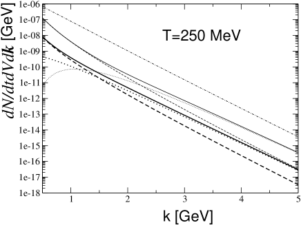
Figure 1: The synchrotron contribution to the photon emission rate $dN/dtdVd\mbox{{\bf k}}$ from $q\to\gamma q$ (dashed) and $q\bar{q}\to\gamma$ (dotted) processes and their sum (solid) at $T=250$ MeV and $eB=m_{\pi}^{2}$ obtained with (thick lines) and without (thin lines) the effect of multiple scattering. The dash-dotted line shows the contribution from the LO $2\to 2$ processes.

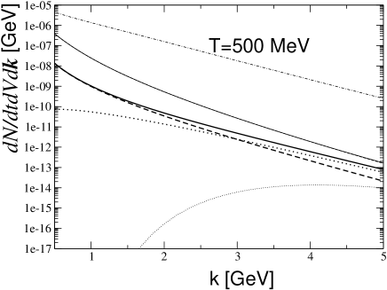
Figure 2: The synchrotron contribution to the photon emission rate $dN/dtdVd\mbox{{\bf k}}$ from $q\to\gamma q$ (dashed) and $q\bar{q}\to\gamma$ (dotted) processes and their sum (solid) at $T=500$ MeV and $eB=m_{\pi}^{2}$ obtained with (thick lines) and without (thin lines) the effect of multiple scattering. The dash-dotted line shows the contribution from the LO $2\to 2$ processes.

The magnetic field in the noncentral $AA$ collisions is mostly perpendicular to the reaction plane (this direction corresponds to $y$ axis, if $x$ axis is directed along the impact parameter of $AA$ collisions). For this reason the transverse (to the quark momentum) component of the Lorentz force is $\propto\cos(\theta)$. This fact leads naturally to a strong azimuthal asymmetry $v_{2}$ for the synchrotron radiation T1 . This effect can be only observed if the relative contribution of the synchrotron mechanism to the photon emission rate is not very small.

For Au+Au collisions at $\sqrt{s}=0.2$ TeV the typical value of the magnetic field at $b\sim 6$ fm and proper time $\tau\sim 0.2$ fm is $eB\sim 0.1m_{\pi}^{2}$ Z_B . We perform numerical calculations for more optimistic value $eB=m_{\pi}^{2}$. In Figs. 1, 2 we present the results for the effect of the magnetic field on the photon emission rate for $T=250$ and $500$ MeV. We show the results separately for bremsstrahlung and annihilation and for their sum. We present also the curves obtained neglecting the effect of multiple scattering ($\Omega=0$). For the comparison we present in Figs. 1, 2 the contribution of the LO mechanisms in the form obtained in AMY1 . One sees that multiple scattering suppresses strongly the contribution of the synchrotron radiation. The curves for the synchrotron mechanism go considerably below the ones for the LO contribution. And for a version with multiple scattering the contribution of the synchrotron mechanism turns out to be practically negligible as compared to the LO mechanism. We see that even for our clearly too optimistic value of the magnetic field the effect of the synchrotron mechanism is very small. For more realistic field $eB\sim 0.1m_{\pi}^{2}$ the synchrotron contribution is smaller by a factor of $\sim 10^{2}$. Thus, one can conclude that the effect of the magnetic field cannot be important for photon emission in $AA$ collisions.

IV Summary

We have studied the influence of the magnetic field on the photon emission rate from the QGP. We find that even for clearly too optimistic assumption on the magnitude of the magnetic field ($eB\sim m_{\pi}^{2}$) the effect of magnetic field is very small, and for more realistic fields ($eB\sim 0.1m_{\pi}^{2}$) the effect is practically negligible. For this reason we conclude that the synchrotron mechanism cannot solve “the direct photon puzzle”. Thus, our calculations do not support the results of the recent analysis T1 , where a rather large effect of magnetic field was found.

References

References

• (1) E.V. Shuryak, Phys. Lett. B78 (1978) 150.
• (2) A. Adare et al. [PHENIX Collaboration], Phys. Rev. Lett. 104, 132301 (2010) [arXiv:0804.4168].
• (3) A. Adare et al. [PHENIX Collaboration], Phys. Rev. Lett. 109, 122302 (2012) [arXiv:1105.4126].
• (4) A. Adare et al. [PHENIX Collaboration], Phys. Rev. C91, 064904 (2015) [arXiv:1405.3940].
• (5) J. Adam et al. [ALICE Collaboration] Phys. Lett. B754, 235 (2016) [arXiv:1509.07324].
• (6) K. Tuchin, Phys. Rev. C91, 014902 (2015) [arXiv:1406.5097].
• (7) P.B. Arnold, G.D. Moore, and L.G. Yaffe, JHEP 0112, 009 (2001) [hep-ph/0111107].
• (8) B.G.Β Zakharov, JETPΒ Lett. 63, 952 (1996); ibid 65, 615 (1997); 70, 176 (1999); Phys.Β Atom.Β Nucl. 61, 838 (1998).
• (9) P. Aurenche and B.G. Zakharov, JETP Lett. 85, 149 (2007) [hep-ph/0612343].
• (10) P. Aurenche, F. Gelis, and H. Zaraket, Phys. Rev. D61, 116001 (2000) [hep-ph/9911367].
• (11) R. Baier, H. Nakkagawa, A. Niegawa, and K. Redlich, Z. Phys. C53, 433 (1992).
• (12) P. Aurenche, F. Gelis, and H. Zaraket, JHEP 0205, 043 (2002).
• (13) N.N.Β Nikolaev and B.G.Β Zakharov, Z. Phys. C49, 607 (1991); ibid., C53, 331 (1992).
• (14) R.Β Baier, Y.L.Β Dokshitzer, A.H.Β Mueller, S.Β PeignΓ©, and D.Β Schiff, Nucl.Β Phys.Β B483, 291 (1997); ibid. B484, 265 (1997); R.Β Baier, Y.L.Β Dokshitzer, A.H.Β Mueller, and D.Β Schiff, Nucl.Β Phys.Β B531, 403 (1998).
• (15) R. Baier, Nucl. Phys. A715, 209 (2003) [hep-ph/0209038].
• (16) B.G.Β Zakharov, JETP Lett. 93, 683 (2011) [arXiv:1105.2028].
• (17) B.G.Β Zakharov, JETP Lett. 96, 616 (2013) [arXiv:1210.4148].
• (18) B.G. Zakharov, J. Phys. G40, 085003 (2013) [arXiv:1304.5742].
• (19) R.P. Feynman and A.R. Hibbs, Quantum Mechanics and Path Integrals, McGRAW–HILL Book Company, New York 1965.
• (20) V.N.Β Baier and V.M.Β Katkov, JETP 26, 854 (1968).
• (21) B.G. Zakharov, Phys. Lett. B737, 262 (2014) [arXiv:1404.5047].