Arrival Times of Gravitational Radiation Peaks for Binary Inspiral

Abstract

Modeling of gravitational waves (GWs) from binary black hole inspiral brings together early post-Newtonian waveforms and late quasinormal ringing waveforms. Attempts to bridge the two limits without recourse to numerical relativity involve predicting the time of the peak GW amplitude. This prediction will require solving the question of why the peak of the “source,” i.e., the peak of the binary angular velocity, does not correspond to the peak of the GW amplitude. We show here that this offset can be understood as due to the existence of two distinct components of the radiation: the “direct” radiation analogous to that in flat spacetime, and “scattered” radiation associated with curved spacetime. The time dependence of these two components, and of their relative phases determines the location of the peak amplitude. We use a highly simplified model to clarify the two-component nature of the source, then demonstrate that the explanation is valid also for an extreme mass ratio binary inspiral.

I Overview

I.1 Introduction and Summary

The recent detections of gravitational radiation events GW150914 GWPRL1 and GW151226 GWPRL2 from black hole binary inspiral has underscored the importance of understanding the theoretical predictions of the waveforms for such processes. Numerical relativity, the computation of the Einstein’s nonlinear equations NR , has played an important role in generating these predictions, but there is a wide range of binary parameters, and studying an appropriately large and finely spaced set of waveforms requires a more efficient methodology to supplement numerical relativity. One such methodology is the effective-one-body approximation (EOB) EOB1 ; EOB2 ; BB , used together with the linear equations of the extreme mass ratio particle-perturbation technique BBHKOP ; TBKH and numerical relativity PBBBKPS .

In the EOB model, two different techniques are used to generate a full waveform signal from a black hole binary system and the results are amplitude and phase matched. In the early epoch (inspiral-plunge) of the binary’s evolution, an EOB Hamiltonian system is evolved and the waveform is computed using an inspiral-plunge trajectory. For the late (merger-ringdown) epoch, the early epoch waveform is matched to a linear superposition of several quasi-normal modes. The precise moment in the binary’s evolution at which this matching is performed is thus a very critical matter in the EOB approach. In the original EOB work EOB1 ; EOB2 it was argued that this matching should be performed close to the light ring where the orbital frequency peaks; thus, the peak of the waveform amplitude was identified with the light ring as well.

The fact that these two peaks do not actually align has been a complication in this program. Particularly troublesome has been the dependence of the peak offsets on the orbital frequency, and the fact that different (spin-weighted) spherical harmonic modes have significantly different offsets BBHKOP ; TBKH ; PBBBKPS . In the EOB papers a time delay is defined, $\Delta t^{\ell,m}_{\rm peak}=t^{\ell,m}_{\rm peak}-t^{\Omega}_{\rm peak}$, where $t^{\ell,m}_{\rm peak}$ is the time at which the peak of the ${\ell,m}$ mode of radiation is observed, and $t^{\Omega}_{\rm peak}$ is the time at which radiation would be observed from the maximum of the particle’s angular velocity. In most cases (i.e. results from numerical relativity and particle perturbation theory models), this delay is negative; the peak radiation is earlier than the radiation from the peak of angular velocity.

Such studies have raised the question why there should be a peak offset, that is, why the apparent peak of the supposed source of radiation does not align with the peak of the radiation generated. Not only would an answer satisfy scientific curiosity, but it could lead to an effective way of predicting the peak offsets. It has been suggested ScottField that the offset, and its dependence on angular frequency, might be explained as manifestations of the energy dependence of the scattering of gravitational radiation off the curvature potential curvpot created by the black holes.

In this paper we will answer that question by exploiting an approach we have recently developed PNK . In that approach, we use the Fourier domain Green function (FDGF) for a very simple model in which we replace the curvature potential with a simplified truncated dipole potential (TDP) tdp . In our approach, we use point particle trajectories, but we do not require them to be analogs of geodesics. This greater freedom to vary trajectories, combined with the simplification from the TDP model, gives transparency to the problem of the location of the radiation peak, and its dependence on angular velocity.

The clear picture that is revealed is that the outgoing radiation consists of two components. One component, the quasinormal or scattered radiation, is due to the motion through the strong field spacetime (equivalently, motion in the neighborhood of the peak of the curvature potential). The second component is the “direct radiation,” radiation that has little to do with the curved spacetime, and can be fully ascribed to the motion of the particle as if it were in flat spacetime. The peak radiation is a result of the combination of the two components.

Through the use of numerical evolution codes we have investigated whether this picture applies to the extreme mass-ratio inspiral (EMRI) problem in the Schwarzschild geometry. Although the direct and scattered contributions cannot be separated in an evolution code, the character of the results clearly indicates that this picture does apply. Further study is appropriate to the applicability to the inspiral of comparable mass holes, but the indications are strong that here too it applies.

The remainder of this paper is organized as follows. In Sec. II we review the features of the TDP/FDGF model that are most relevant to the investigation of the peak location. Numerical results from that model are presented in Sec. III, and a tentative explanation is presented of the location of the amplitude peak. Section IV then shows that the qualitative features of the peak location are the same for the EMRI models in the Schwarzschild spacetime as in the TDP model. Conclusions are given in Sec. V.

II The TDP/FDGF Methodology

When analyzed into spherical harmonics of index ($\ell,m$) perturbations of Schwarzschild black holes can be formulated in terms of a radiation field (scalar, electromagnetic, gravitational,…) satisfying an equation of the form

$$\frac{\partial^{2}\Psi_{\ell m}}{\partial r^{*2}}-\frac{\partial^{2}\Psi_{\ell m}}{\partial t^{2}}-V_{\ell}(r^{*})\Psi_{\ell m}=S_{\ell m}(r^{*},t)\,.$$ (1)

Here $r^{*}$ is the Regge-Wheeler RW57 “tortoise coordinate” which places the event horizon at $r^{*}=-\infty$, and approaches the ordinary Schwarzschild areal radius $r$ when $r^{*}$ is much larger than the mass $M$. The details of the curvature potential $V_{\ell}(r^{*})$ depend on which perturbation field is being represented, but in all cases $V_{\ell}(r^{*})\rightarrow\ell(\ell+1)/r*^{2}$ as $r^{*}/M\rightarrow\infty$, and $V_{\ell}(r^{*})\rightarrow\mbox{const}\times e^{r^{*}/2M}$ as $r^{*}/M\rightarrow-\infty$. In the TDP model of a scalar field $\Psi$, the radial variable is replaced by a variable $x$ that ranges from $-\infty$ to $+\infty$, and the $\ell=1$ curvature potential is replaced by

$$V=\left\{\begin{array}[]{cl}\ell(\ell+1)/x^{2}=2/x^{2}&{\rm for}\ x>x_{0}\\ 0&{\rm for}\ x<x_{0}\end{array}\right.\,.$$ (2)

The potential “edge,” or peak, at $x_{0}$, is the TDP proxy for the peak of the curvature potential approximately at the $r=3M$ location of the circular photon orbit, the “light ring” (LR), in the Schwarzschild geometry.

A scalar field $\Psi$ is imagined to have a point particle source, so that the time domain equation for $\Psi$ is

$$\frac{\partial^{2}\Psi}{\partial x^{2}}-\frac{\partial^{2}\Psi}{\partial t^{2}}-V(x)\Psi=f(t)\delta\left(x-F(t)\right)\,.$$ (3)

In the source, the function $F(t)$ represents the position of the point particle as a function of time. The function $f(t)$ can represent a time-dependent modulation of the source; we shall use it below to account for the effects of angular motion. The Fourier domain Green function ${\cal G}$ for a particle at $x=\widetilde{F}$ satisfies

$$\frac{\partial^{2}{\cal G}}{\partial x^{2}}+\left(\omega^{2}-V(x)\right){\cal G}=\delta(x-\widetilde{F}),$$ (4)

and with it the solution to Eq. (3) takes the form

$$\Psi(t,x)=\frac{1}{2\pi}\int_{-\infty}^{\infty}\int_{-\infty}^{\infty}\int_{-\infty}^{\infty}e^{-i\omega(t-T)}{\cal G}(x,\widetilde{F};\omega)f(T)\delta(\widetilde{F}-F[T])\,d\omega\,d\widetilde{F}\,dT\,.$$ (5)

II.1 Model details

In particle-perturbation studies, and in our TDP model, there is no constraint that the particle trajectory be associated with geodesic motion, so that we are free to choose families of trajectories that best probe the questions of interest. For the “radial,” i.e., “$x$” motion radial , we choose $F(t)$ to be a relatively simple algebraic function

$$F(t)=\left\{\begin{array}[]{cl}a_{0}+\tau-\left(t^{3}+\tau^{3}\right)^{1/3}&t>0\\ a_{0}&t<0\,.\end{array}\right.$$ (6)

The two parameters are $a_{0}$, the initial $x$ position of the particle, and $\tau$, the timescale on which the particle accelerates. Note that the particle starts, at $t=0$, with zero velocity and acceleration, so that the source can be considered to have been stationary prior to $t=0$.

If the TDP model is an analog of a particle with azimuthal position $\phi=\widetilde{\phi}(t)$ we take $f(T)=e^{i\widetilde{\phi}(T)}$ . The reason behind this choice is as follows: The function $\Psi$ in Eq. (3) is actually the analog of the coefficient function $\Psi_{\ell m}(t,r)$ of a spherical harmonic expansion, confined to $\ell=1$. In the case of radial motion only the $m=0$ component is nonzero (with the radial motion taken along the $\theta=0$ axis of the spherical coordinates). In the case of angular motion, $\theta$ is taken as $\pi/2$, and only the $m=\pm 1$ components are nonzero. The choice $f(T)=e^{\mp i\widetilde{\phi}(T)}$ corresponds to $m=\pm 1$.

In order to represent a particle that is stationary in angular as well as radial position prior to the $t=0$ start of motion, we choose as our model

$$\tilde{\phi}(t) =\omega_{\rm max}T_{\rm peak}\,\frac{e^{3}}{81}\left[e^{-z}(-6-6z-3z^{2}-z^{3})+6\right]$$ (7a)

$$z \equiv 3t/T_{\rm peak}\,.$$ (7b)

For this choice, the angular velocity is

$$\omega\equiv\frac{d\tilde{\phi}}{dt}=\omega_{\rm max}\,\frac{e^{3}}{27}\left(z^{3}e^{-z}\right)\,.$$ (8)

The angle $\tilde{\phi}$, and the angular velocity and angular acceleration, are zero at $t=0$, so that for its angular motion as well as its “radial” motion, the particle can be taken to have been stationary prior to $t=0$. Of particular importance is the fact that we can independently specify the parameter $\omega_{\rm max}$, the maximum angular velocity, and $T_{\rm peak}$, the particle time at which that maximum is achieved.

II.2 Closed form solution

For the TDP model, the FDGF can be found in closed form for each of the relative positions of the potential “edge,” $x_{0}$, the particle location $\widetilde{F}$, and the location $x$ at which the field is being calculated. Since we are interested in the radiation region, we consider $x$ to be unbounded. We are left then with the case in which $\widetilde{F}>x_{0}$, the particle, in its inward motion has not yet crossed the edge at $x_{0}$, and $\widetilde{F}<x_{0}$, the case in which the particle has already passed inside the edge. In our numerical studies we have found that the early retarded time peak of the outgoing radiation, the peak of interest as an analog of the Schwarzschild problem, is generated by the motion of the particle before it passes inward past the edge. In this case, the radiative part of the solution (i.e., the part to leading order in $1/x$) has the form

$$\psi(t,x)=\frac{1}{2}\,\int_{T_{2}}^{T_{1}}\frac{u-T}{F(T)}f(T)\,dT-\,\frac{1}{2}\,\int_{-\infty}^{T_{2}}\,e^{-\gamma_{I}}\left[-(\cos{\gamma_{R}}+\sin{\gamma_{R}})+\frac{2x_{0}}{F(T)}\,\cos{\gamma_{R}}\right]f(T)\,dT\,.$$ (9)

Note that this solution is good only for retarded time $u\equiv t-x$ less than or equal to the critical value $u_{\rm cross}\equiv T_{\rm cross}-x_{0}$, where $T_{\rm cross}$ is the time at which the particle reaches $x_{0}$.

In the solution given by Eq. (9) the $t,x$ dependence is contained in the dependence on retarded time $u\equiv t-x$ of the integration limits $T_{1},T_{2}$ and of the real and imaginary parts of $\gamma$, given by

$$\gamma_{R}=\omega_{R}\left(u-T-F(T)+2x_{0}\right)\quad\quad\gamma_{I}=\omega_{I}\left(u-T-F(T)+2x_{0}\right)\,.$$ (10)

Here $\omega_{R}$ and $\omega_{I}$ are the real and imaginary part of the TDP quasinormal frequency. For the TDP, there is only a single QN frequency, a frequency which turns out to have real and imaginary parts of equal size

$$\omega_{R}=\omega_{I}=1/(2x_{0})\,.$$ (11)

The notation and meaning of $T_{1}$ and $T_{2}$ are taken from our paper, Ref. PNK , and are defined by

$$T_{1}=u+F(T_{1})\quad\quad T_{2}=u+2x_{0}-F(T_{2})\,,$$ (12)

and are illustrated by the spacetime cartoon in Fig. 1 from our earlier paper PNK . This figure, and Eq. (12)

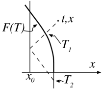
Figure 1: A spacetime diagram showing the meaning of $T_{1}$ and $T_{2}$. The bold line represents the trajectory of the particle $x=F(T)$; the dashed lines are radial characteristics.

show that $T_{1}$ is simply the causality limit; the observation event cannot be influenced by a point on the trajectory at a later retarded time. The meaning of the $T_{2}$ limit is more subtle; it restricts the second integral to times less than those for which the particle source had time to “bounce” its influence off the potential edge and reach the observation point $t,x$. The $T_{2}$ upper limit, and the presence of $\gamma_{R},\gamma_{I}$ in the second integral are strong signs that the second integral represents the scattering of the particle influence from the potential.

The first integral has a very different interpretation. The integrand suggests that this integral represents “direct” radiation, with no reference to the quasinormal modes or to potential scattering explainT2 . We can make this connection much more convincing by considering the direct scalar radiation generated by a particle in flat spacetime. This result is

$$\psi_{\rm flat}(t,x)=\frac{1}{2}\,\int_{\bar{T}_{2}}^{\bar{T}_{1}}\frac{u-T}{F(T)}f(T)\,dT\,,$$ (13)

where

$$\bar{T}_{1}=u+F(\bar{T}_{1})\quad\quad\bar{T}_{2}=u-F(\bar{T}_{2})\,.$$ (14)

The first integral in Eq. (9), rather clearly, represents direct radiation with the $x_{0}$ edge replacing the coordinate origin as the location at which ingoing radiation is reversed and sent outward. We shall, henceforth, refer to the first integral in Eq. (9) as the direct contribution to the radiation and shall refer to the second integral as the scattered, or QN contribution.

III The TDGF/TDP Results

With $f(T)=\exp{(-i\tilde{\phi}(T))}$, Eq. (9) gives us $\psi_{1,1}(t,x)$, the $\ell,m=1,1$ spherical harmonic part of the radiation; with $f(T)=\exp{(+i\tilde{\phi}(T))}$, it gives us the $\ell,m=1,-1$ part. We present results in this section for the amplitude of the radiation

$$\psi_{\rm amp}=|\psi_{1,1}|=|\psi_{1,-1}|\,.$$ (15)

These results were also computed with the evolution code described in Sec. IV, in which the Schwarzschild curvature potential was replaced by the TDP potential. This check showed accurate agreement with the results of the FDGF integration.

We shall focus on a particular radial motion, that for the following trajectory parameters in Eq. (6): $a_{0}=4$, $\tau=10$, $x_{0}=1$ scaling . For these parameters, the particle, on its inward journey, crosses the $x_{0}$ edge at $T_{\rm cross}=10.6177$, with a rather relativistic speed $v_{\rm cross}=|dF/dT|_{\rm cross}=0.6671$. We have checked other “radial” motions, including trajectories with much smaller values of $v_{\rm cross}$, to be sure that the observations in this paper apply rather generally.

There are two important considerations in the choice of the parameters for the angular motion in Eq. (7). First, for the Schwarzschild EMRI case the maximum of the angular velocity is at the $r=3M$ light ring. The TDP analog of the light ring is the potential edge at $x_{0}$. The problem is that this is also where the maximum radiation would be expected due to features of the problem that have nothing to do with angular motion. (This expectation will be confirmed by results below.) Thus, if we use the most physical choice for $T_{\rm peak}$, the choice $T_{\rm peak}=T_{\rm cross}$, it will be impossible to disentangle the effect of angular motion from other elements of the generation of radiation. For that reason we choose $T_{\rm peak}=T_{\rm cross}+\mbox{shift}$, and make three choices of the value of the shift parameter.

The second important consideration is the scale for $\omega_{\rm max}$. Intuitively we (correctly) suspect that too small a value of $\omega_{\rm max}$ will mean that the angular motion will be irrelevant; the properties of the radiation will differ very little from those for radial infall. We suggest that angular motion will become significant when $\omega_{\rm max}$ is of the order of the quasinormal frequency $1/2x_{0}$. A justifiable basis for such intuition is that the only length scale in the model is $x_{0}$, so the only scale for frequency is $1/x_{0}$. Full clarification will come later in this section.

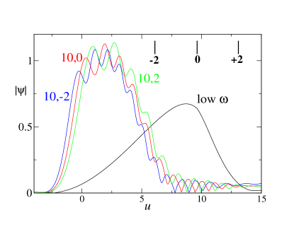
Figure 2: Amplitude as a function of retarded time $u\equiv t-x$ for the standard model of “radial” infall with $a_{0}=4$, $\tau=10$, $x_{0}=1$. The curve marked “low $\omega$” represents all models with $\omega_{\rm max}\leq 0.1$. The numerical markings on the higher curves indicate the value of $\omega_{\rm max}$ and the shift, respectively. The short vertical bars indicate the retarded time at which a signal would be received from the particle when moves at $\omega_{\rm max}$. The bars are marked with the value of the applicable shift.

We first dispense with the high and low cases in Fig. 2. For $\omega_{\rm max}\leq 0.1$, all curves, for any of the shifts, are indistinguishable, and are represented in Fig. 2 by the single curve denoted “low $\omega$.” This simply confirms the understanding that for such values the angular motion is irrelevant to the generation of the peak radiation. The peak of the amplitude of this curve is at $u=8.7$, reasonably close to the retarded time $u_{\rm cross}=T_{\rm cross}-x_{0}=9.6177$ corresponding to the particle crossing the potential edge. This is also the time when the particle achieves its maximum angular velocity for the choice shift=0. The choices shift=$\pm 2$, however, correspond to very different retarded times, as indicated by the vertical bars in the figure. The fact that the low $\omega$ curves are not influenced by a change in the shift choice, emphasizes that these results show no effects of angular motion.

The higher curves in Fig. 2 show the radiation for $\omega_{\rm max}=5$, and for shifts 0,$\pm 2$ (given as the second index in each curve’s label). These curves do not all have a well defined peak, but a few points remain quite clear: (i) The location of the region of peak amplitude is significantly earlier than the time that peak radiation would be expected (the vertical bars in the figure) if the maximum amplitude were related to the maximum angular velocity. (ii) The displacement of the amplitude peaks has no strong correlation with the shifts in the peak angular velocity. (iii) The curves show an oscillatory behavior throughout that can be shown to have periodicity that is accurately correlated with the particle angular motion at the corresponding retarded time, after a correction for the doppler shift PNK . (iv) The fact that there are oscillations shows that the radiation cannot be due only to the angular motion. (The $e^{i\tilde{\phi}(t)}$ source motion has a constant magnitude.) The oscillations are proof that the total radiation is a mixture of contributions associated with the angular motion and those that are not.

The qualitative nature of the results in Fig. 2 for $\omega_{\rm max}=5$ are representative of all high $\omega$ models, all models with $\omega_{\rm max}$ greater or equal to around 4. At higher $\omega_{\rm max}$, the curves have a higher frequency oscillation, but are located in the same general range of retarded time.

Figure 3 shows the results for the interesting intermediate range of $\omega_{\rm max}$. Clearly, as $\omega_{\rm max}$ increases the nature of the curves goes through a transition from the low $\omega_{\rm max}$ to the high $\omega_{\rm max}$ curves of Fig. 2. In these results the peak amplitude is not correlated with the retarded time of the peak angular velocity, and is generally earlier.

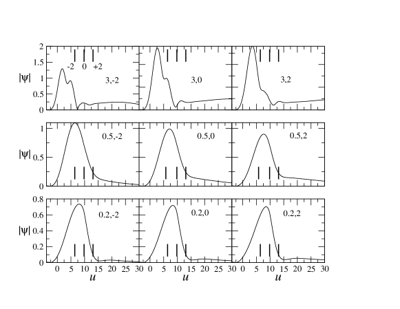
Figure 3: Amplitude as a function of retarded time for the standard model, as in Fig. 2, but here for intermediate values of $\omega_{\rm max}$. As in Fig. 2, curves are labeled with indices of $\omega_{\rm max}$ and shift. The bold vertical bars represent the retarded times corresponding to the peak of $\omega$, for shifts of $0,\pm 2$, as labeled in the first graph. Note that the QN frequency’s value is $0.5$ for this model.

By exploiting the simplicity of the TDP/FDGF mathematics we can analyze the source of this behavior. Figure 4 shows the radiation amplitudes separately for the direct and the scattered components of the total, i.e., for the amplitudes computed separately from the first and second integrals in Eq. (9).

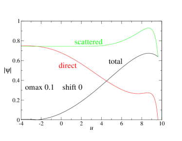
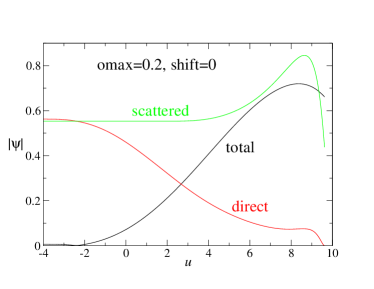
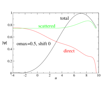
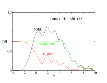
Figure 4: The total radiation complitude, along with the amplitudes of the scattered component, and of the direct radiation component, for several different values of $\omega_{\rm max}$.

The sequence of curves, in Fig. 4, from low to high values of $\omega_{\rm max}$ shows interesting trends. At high $\omega_{\rm max}$, the scattered and direct components are in phase at the peak of the total radiation. The total amplitude, in fact, is very nearly the sum of the two individual amplitudes. On the other hand, for low values $\omega_{\rm max}$, the two components of radiation appear to be totally out of phase.

What is most important to an explanation about the results is that in Fig. 4 the direct contribution falls off at late retarded times, times approaching $u_{\rm cross}$, the retarded time corresponding to the particle crossing the $x_{0}$ edge. The explanation of why the direct radiation falls off approaching $u_{\rm cross}$ can be extracted from the simplicity of the first integral in Eq. (9), the integral for the direct radiation. The definitions in Eq. (12) show that the range of integration, $T_{1}-T_{2}$, shrinks to zero as $u\rightarrow u_{\rm cross}$. The physical meaning of this is clear in the cartoon in Fig. 1 which shows a direct, and a “bounced” radial characteristics from particle to observer. As the particle approaches the $x_{0}$ edge, the separation of these two paths shrinks. The direct radiation decreases, in fact, because the reflected outgoing radiation from the particle tends to cancel the radiation going directly outward from the particle. As the partice approaches the reflecting edge at $x_{0}$, this cancelation tends to be complete.

There is a general, but not universal tendency for the scattered radiation, like the direct radiation, also to fall off as $u\rightarrow u_{\rm cross}$. What is central, however, to the explanation of the early amplitude peak is that the direct radiation, an important part of the total radiation, must vanish at $u_{\rm cross}$, thereby forcing the peak amplitude to occur earlier.

This explanation can be reinforced by a consideration of the relative phases of the two radiation components. At the start of motion ($u=-4$ in Fig. 4) there can be no radiation; the particle is starting with no radial or angular acceleration. It is interesting that neither the direct nor the scattered component is zero at the start, but their sum must be, since the total radiation must vanish. All curves in Fig. 4 therefore start with the two components out of phase, but the subsequent development is quite different for low and for high $\omega_{\rm max}$. For low $\omega_{\rm max}$, the two components remain out of phase. The fact that for low $\omega_{\rm max}$ the amplitude peak occurs at “late” times, not much before $u_{\rm cross}$, can be ascribed to the vanishing of the subtraction of the out of phase direct radiation. (The rise in the scattered radiation at low $\omega_{\rm max}$ in Fig. 4 is not universal; it is not seen in slower infall models.) At high $\omega_{\rm max}$, the angular modulation of both components drives them to be in phase. The higher the value of $\omega_{\rm max}$, the more tightly are the two components locked in phase. The physically required decrease in the direct component as $u$ approaches $u_{\rm cross}$ along with the observed tendency for the scattered component also to decrease explains why the amplitude peak at high $\omega_{\rm max}$ is at early times.

It now remains to be seen whether this explanation applies to the Schwarzschild problem as well as to our TDP toy model.

IV The EMRI/Schwarzschild Results

As pointed out in Sec. II, the mathematics of the true Schwarzschild problem has an obvious similarity to that of the TDP model, but there are additional reasons to believe that the picture of the previous section, based on TDP, applies also to Schwarzschild. In particular, the two integrals in Eq. (9) arise from the poles of the Green function ${\cal G}(x,\widetilde{F};\omega)$. The direct integral arises from the $\omega=0$ pole, and the scattered radiation integral arises from the pole at the QN frequency. The structure of the Green function for Schwarzschild is similar, with a pole for the dominant QN mode (as well as for all other QN modes for a given multipole) and a singularity at $\omega=0$, although the Schwarzschild Green function has additional structure SchwGF .

The computation of radiation from the Schwarzschild FDGF is much more difficult than that for the TDP FDGF, so we take advantage of the availability of a time-domain evolution code PNK . With that code, we repeat the same study as the one performed in the previous sections in the context of the TDP model, for the case of gravitational wave (GW) emission from EMRIs into a Schwarzschild black hole of mass $M$. Once again, we do not restrict ourselves to physical inspiral trajectories and instead use the equivalent of the radial and angular motion used in Sec. II and III with the tortoise coordinate

$$r^{*}=r+2M\ln{(r/2M-1)}\,$$ (16)

replacing $x$, and the LR location $r^{*}=1.6317M$ (equivalent to $r=3M$) in place of $x_{0}$. Here and throughout we use the notation of the textbook by Misner, Thorne and Wheeler MTW , and in particular use $c=G=1$.

IV.1 Model details

For the radial motion, we use the same “cubic” trajectory as was used in the TDP model of the previous section, although with different parameter choices. All models were chosen to have radial motion with $a_{0}=38.6114M$ and $\tau=600M$, and in all cases the particles pass the LR at time $t=T_{\rm LR}=348.90M$, with a radial speed $v_{\rm LR}=0.3$ (From our previous work PNK we know that these parameters allow accurate evolutions.). For the angular motion, we use the same law as for the TDP models in Eqs. (7).

We had noted in our previous paper PNK that the angular velocity must have its peak at the light ring. For that reason, our default choice will be to have $T_{\rm peak}$ correspond to the time ($T_{\rm LR}$) at which the particle crosses the LR. We will, however, allow for exploration of sensitivity by taking, in analogy with the TDP results, $T_{\rm peak}=T_{\rm LR}+\mbox{shift}$, in which we will take shift to be $\pm 7M$ in addition to $0$. Note that all GW waveforms were extracted at $r^{*}=200M$. Extraction at $r^{*}=\infty$, equivalent to the “extraction” in the TDP model, would make an insignificant difference.

IV.2 Computational results

We follow the pattern of the previous section and start with the cases of limiting $\omega_{\rm max}$. In Fig. 5 we show such limiting cases for shift=0 (i.e., for the maximum of the angular velocity at the LR). These results show the dominant $\ell,m=2,2$ gravitational wave amplitude, for the $M\omega_{\rm max}$ values 0.7 and 0.01, as indicated. In order to illustrate the peak location most clearly, the amplitude dependences on retarded time reported in Fig. 5, and below in Fig. 6, are normalized to peak amplitude unity. It is worth noting that gravitational wave amplitudes depend much more on $\omega_{\rm max}$, than in the TDP case. This strong dependence is due to the strong dependence on $\omega$ inherent in the the stress-energy source. Computations, not reported here, with a scalar field in the Schwarzschild background, rather than gravitational perturbations, show behavior qualitatively similar to the TDP model for the dependence of amplitude on $\omega_{\rm max}$.

In Fig. 5 the curve of $\omega_{\rm max}=0.01/M$ stands also for all curves of smaller $\omega_{\rm max}$. For all such values there is negligible angular motion during the generation of radiation, and hence no dependence on $\omega_{\rm max}$. In the same spirit, the result for $\omega_{\rm max}=0.7/M$ shows the qualitative nature of the amplitude for high $\omega_{\rm max}$; at larger values of $\omega_{\rm max}$, the results have more rapid oscillations, but the region of the peak amplitude does not change.

A bold vertical bar at retarded time $u=348.9$ indicates the retarded time corresponding to $T=T_{\rm LR}$ and the maximum of the angular velocity, for zero shift. As in the TDP case, the low $\omega_{\rm max}$ result has a peak at approximately that retarded time while the high $\omega_{\rm max}$ amplitude peak is much earlier than that retarded time.

Figure 6 is the Schwarzschild analog of the TDP results in Fig. 3. The amplitude as a function of retarded time is presented for a sequence of intermediate values of $\omega_{\rm max}$, showing the transition from low $\omega_{\rm max}$ to high $\omega_{\rm max}$. The qualitative nature of this transition is very similar to that for the TDP results. (Again, it should be noted that in Fig. 6, unlike Fig. 3, all peak amplitudes are normalized to unity.)

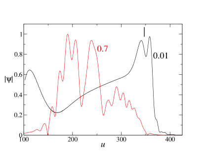
Figure 5: The (normalized) amplitude for the $\ell,m=2,2$ outgoing GW radiation for the particle trajectories in Schwarzschild spacetime as described in the text. Curves are marked with value of $\omega_{\rm max}$, the peak angular velocity of the particle, in units of $1/M$. The bold vertical bar in the upper right of the graph indicates the retarded time corresponding to the passage of the particle through the LR.

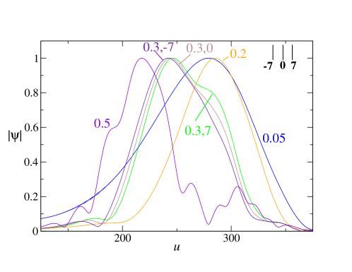
Figure 6: The (normalized) amplitude of the outgoing radiation for the particle trajectories in Schwarzschild spacetime as described in the text. Curves are marked with value of $M\omega_{\rm max}$, the peak angular velocity of the particle. For $M\omega_{\rm max}=0.3$ the second index in the curve labels gives the value of the shift, the time, in units of $M$, by which the angular velocity maximum has been shifted. In the upper right hand corner, vertical bars indicate the retarded times corresponding to the angular velocity maximum for shifts $0,\pm 7$ in units of $M$. Note that the QN frequency is $0.37$ in units of $1/M$. It is clear that only when the value of $\omega_{\rm max}$ is comparable to the QN frequency, the the GW peaks, shift to earlier times.

IV.3 Relationship to previously observed GW peak offsets

As stated before, the fact that the (retarded) peak of the orbital frequency and the peak of the gravitational radiation do not align has been known for some time, both in the context of EMRIs BBHKOP ; TBKH and in the comparable-mass binary systems PBBBKPS . In addition, it has also been noted that different spin-weighted spherical harmonic modes of the gravitational waveform peak at different times (see for example, Table II in Ref. BBHKOP for the Schwarzschild EMRI case). It has also been known that in the Kerr geometry the radiation peak offset is strongly dependent on the spin $a/M$ (see Table III in Ref. BBHKOP ). In this section, we argue that the results previously reported about the peak misalignment are consistent with the central observations in the current work.

First, consider the case of gravitational wave emission from particle motion in Schwarzschild spacetime. Examining the dependence of the peak offset for fixed $\ell$ modes (in particular, $\ell=2$) in Table II of Ref. BBHKOP suggests that the higher $m$-modes peak at earlier times. This is exactly what we have pointed out in the previous sections of this paper. In our TDP model, we changed the value of the angular frequency instead, but note that is mathematically equivalent to changing the $m$-mode, of course. (It is important to fix the value of $\ell$ for a proper comparison with our current work, in order for the potential function to stay unchanged.)

In the Kerr context, Table III in Ref. BBHKOP depicts the peak offset of the $\ell=m=2$ mode as a function of the Kerr parameter $a/M$. It is clear from those data that as $a/M$ increases the gravitational waveform peaks earlier. Once again, this is consistent with the expectations from the previous sections in this work; a higher value of $a/M$ implies higher orbital frequency (a smaller ISCO allows the particle to orbit a lot closer to the Kerr hole) and those cases peak at earlier times. Of course, the Kerr potential is strongly spin-dependent, and that likely plays a role in the timing of the peaks as well. Moreover for the high-spin cases, while the peak offset is large, it is also true that the peak “flattens out” considerably, making it harder to pinpoint its precise location.

As examples of these offsets we present results adapted from Refs. BBHKOP ; TBKH . These results were generated using a high-accuracy and high-performance Teukolsky equation solver in the time-domain, with a point-particle source term mycode . Table 1 shows the delay in the dominant ${\ell,m}=2,2$ mode of gravitational radiation for a particle spiralling in on an equatorial orbit into a Kerr black hole. The value of $a/M$ indicates the spin of the Kerr hole; in the first column, a negative $a/M$ indicates retrograde inspiral. The second column shows the delay between the moment the radiation peaks, and the moment when the radiation arrives from the peak of the angular velocity. For all but the retrograde inspiral, this delay is negative; the peak of the amplitude is earlier than the signal coming from the peak of angular velocity.

This table also shows a comparison of frequencies that are relevant to our explanation of this delay. The third column shows the peak of the angular velocity $d\phi/dt$. The angular velocity is given in units of $1/M$ and multiplied by 2 since the 2,2 radiation produced by angular motion should have frequency twice that of the angular motion. The fourth column, with the quasinormal frequencies for the least damped 2,2 mode shows that this frequency is close to the angular velocity and thus the mechanism for the peak offset is likely to be the same that we have presented in this current work.

V Conclusion

Though peak time offsets have been important in waveform construction, all that has been known is that such a time offset exists and that it is different (a) in the Schwarzschild background for gravitational waves in different multipole modes, and also (b) in the Kerr background for even a given multipole mode, but different values of $a/M$. We know of no claim in the literature that suggests an explanation of this offset, what it depends on, or whether (a) and (b) are related.

In this paper we present insights that provide at least the beginning of an explanation of the peak offset phenomenon. These insights are the results of exploiting the simplicity of a model first explored in our previous paper PNK . In particular, (i) the curvature potential of the Schwarzschild EMRI problem is replaced by a simplified truncated dipole potential; (ii) the source is understood through the Fourier domain Green function; (iii) we do not restrict ourselves to geodesic orbits, but use trajectories that allow us to probe the mechanisms for the generation of radiation.

This simplicity has produced a very simple explanation of why the amplitude peak for low $\omega_{\rm max}$ is at the “expected” late retarded time, but for high $\omega_{\rm max}$ is significantly earlier. In simplest terms, the idea is that the radiation consists of two components, direct radiation and scattered radiation, and that the direct component vanishes at the “expected” retarded time. For low $\omega_{\rm max}$ the two components are out of phase, so the late-time vanishing of the subtracted direct radiation means that the peak, dominated by the scattered radiation, can occur at late times. For high $\omega_{\rm max}$ the two components are in phase. The vanishing of the late-time direct radiation, therefore, removes its addition to the total, and pushes the peak total to earlier times.

The separation of the direct and scattered components of the radiation for the Schwarzschild EMRI problem is not simple, but the qualitative similarity of our results for the TDP and for the Schwarzschild background, both for gravitational waves and for scalar waves (not reported here), makes a strong case that the same mechanism is at work. The case is particularly strong for the claim that the replacement of the Schwarzschild curvature potential by the TDP potential is justified in seeking an explanation.

Further support comes from the details of the Schwarzschild results in the literature. In Table II of the EMRI studies reported for the Schwarzschild background in Ref. BBHKOP , the time by which the amplitude peak precedes the angular velocity peak, for a given $\ell$ mode, increases with the $m$ index of the mode. This increase is mathematically equivalent to increasing the angular velocity. The reported results, then, show that as the angular velocity increases, the peak moves earlier, as in the results we report above, both for the TDP and Schwarzschild models.

Turning to the Kerr case, in Table 1 we present results

$a/M$	$h_{22}$ offset	$2M\omega_{\rm peak}$	$M\omega_{\rm QN}$
-0.9	+2.0	0.18	0.30
0.0	-3.0	0.28	0.37
0.5	-7.0	0.38	0.47
0.9	-40.0	0.64	0.67
0.99	-60	0.84	0.87

Table 1: The time offsets of the $\ell,m=2,2$ peak of radiation from particles spiralling into Kerr black holes with spin parameter $a$, and mass $M$. The second column shows the offset (in units of $M$) by which the GW peak follows the signal from the maximum of the angular velocity. The third column shows twice the peak orbital frequency (in units of $1/M$) of the inspiralling particle. The fourth column is the quasinormal frequency of the dominant (least damped) $\ell,m=2,2$ mode. It is clear that when the last two columns have values that are comparable, a significant offset is observed.

of EMRI studies adapted from Refs. BBHKOP ; TBKH . Of note is the fact that the peak frequency is at a value quite close to that of the real part of the least damped quasinormal frequency for the GW 2,2 mode. These frequencies correspond to the high/intermediate frequencies of Secs. III and IV and this strongly suggests that the same mechanism may be at play in the Kerr case as well.

It remains to be seen whether the strong $a/M$ dependence of the offsets in the Kerr geometry can be fully explained in terms of the same mechanism as in the TDP and Schwarzschild cases. The insights about these peak offsets, as presented in this paper, can most effectively be used in the EOB approach to waveform construction.

VI Acknowledgments

We are greatly indebted to Alessandra Buonanno for her thorough review of an earlier version of this manuscript. Her detailed feedback has significantly improved this current version. We would also like to acknowledge discussions and helpful remarks made by Scott Field, Scott Hughes, and Andrea Taracchini in the context of this work. G.K. acknowledges research support from NSF Grants No. PHY-1303724 and No. PHY-1414440, and from the U.S. Air Force agreement No. 10-RI-CRADA-09.

References

- (1) B.P. Abbott et al. (LIGO Scientific Collaboration and Virgo Collaboration) Phys. Rev. Lett. 116, 061102 (2016).
- (2) B.P. Abbott et al. (LIGO Scientific Collaboration and Virgo Collaboration) Phys. Rev. Lett. 116, 241103 (2016).
- (3) L. Lehner, F. Pretorius, Annual Review of Astronomy and Astrophysics, 52, 661 (2014); V. Cardoso, L. Gualtieri, C. Herdeiro, U. Sperhake, Living Rev. Relativity, 18, 1 (2015); T. Baumgarte, S. Shapiro, Numerical Relativity: Solving Einstein’s Equations on the Computer, Cambridge University Press (2010); M. Shibata, Numerical Relativity, World Scientific Publishing (2015); M. Alcubierre, Introduction to 3+1 Numerical Relativity, Oxford University Press (2008).
- (4) A. Buonanno and T. Damour, Phys. Rev. D 59, 084006 (1999).
- (5) A. Buonanno and T. Damour, Phys. Rev. D 62, 064015 (2000).
- (6) E. Barausse and A. Buonanno, Phys. Rev. D 84, 104027 (2011).
- (7) E. Barausse, A. Buonanno, S.A. Hughes, G. Khanna, S. O’Sullivan, and Y. Pan, Phys. Rev. D 85, 024046 (2012).
- (8) A. Taracchini, A. Buonanno, G. Khanna, and S. A. Hughes, Phys. Rev. D 90, 084025 (2014).
- (9) Y. Pan, A. Buonanno, M. Boyle, L.T. Buchman, L.E. Kidder, H.P. Pfeiffer, M.A. Scheel, Phys. Rev. D 84, 124052 (2011).
- (10) Scott Field, private communication.
- (11) Various authors use different names (“effective potential,” “scattering potential, “curvature potential”) for this potential-like term. See, e.g., W. H. Press, Astrophys. J. 170, L105 (1971); R. H. Price, Phys. Rev. D 5, 2419 (1972); A. Buonanno, AIP Conference Proceedings 968, 307 (2008); F. J. Zerilli, Phys. Rev. Lett. 24, 737 (1970).
- (12) R. H. Price, S. Nampalliwar, and G. Khanna, Phys. Rev. D 93 044060 (2016);
- (13) R. H. Price, Phys. Rev. D 5, 2419 (1972); H.-P. Nollert, Classical and Quantum Gravity 16, 159 (1999).
- (14) T. Regge and J.A. Wheeler, Phys. Rev. 108, 1063 (1957).
- (15) Since there is no physical model connected to the TDP model, the term “radial” is not strictly meaningful, but is convenient.
- (16) The presence of in the first integral might seem to suggest that it does not quite describe direct radiation, because depends on . In the details of the derivation, however, it turns out that at early times, the particle influence propagates inward, reflects off the edge, reverses its sign, and propagates outward. At particle times earlier than , the directly outgoing influence and the influence reflected off the edge cancel.
- (17) The scale in the TDP problem is set by , which can be thought of as playing a role analogous to that of the mass parameter in the Schwarzschild spacetime. In principle, we could express all parameters in dimensionless form, for example, we could use in place of . Since we are choosing , all parameters can be thought of as being de-dimensionalized in this way.
- (18) There are an infinite number of QN frequencies for the Schwarzschild spacetime, and hence an infinite number of corresponding poles in the Schwarzschild GF. In addition, the Schwarzschild GF has a branch point at .
- (19) C. W. Misner, K. S. Thorne, and J. A. Wheeler, Gravitation (W. H. Freeman, San Francisco, 1973).
- (20) L. Burko and G. Khanna, Europhysics Letters 78 60005 (2007); P. Sundararajan, G. Khanna and S. Hughes, Phys. Rev. D 76 104005 (2007); P. Sundararajan, G. Khanna, S. Hughes, S. Drasco, Phys. Rev. D 78 024022 (2008); P. Sundararajan, G. Khanna and S. Hughes, Phys. Rev. D 81 104009 (2010); A. Zenginoglu, G. Khanna, Phys. Rev. X 1, 021017 (2011); J. McKennon, G. Forrester, G. Khanna, Proceedings of the NSF XSEDE12 Conference, Chicago (2012).