Abstract: From spline theory it is well-known that univariate cubic spline interpolation, if carried out in its natural Hilbert space $W_{2}^{2}[a,b]$ and on point sets with fill distance $h$, converges only like ${\cal O}(h^{2})$ in $L_{2}[a,b]$ if no additional assumptions are made. But superconvergence up to order $h^{4}$ occurs if more smoothness is assumed and if certain additional boundary conditions are satisfied. This phenomenon was generalized in 1999 to multivariate interpolation in Reproducing Kernel Hilbert Spaces on domains $\Omega\subset\mathbb{R}^{d}$ for continuous positive definite Fourier-transformable shift-invariant kernels on $\mathbb{R}^{d}$. But the sufficient condition for superconvergence given in 1999 still needs further analysis, because the interplay between smoothness and boundary conditions is not clear at all. Furthermore, if only additional smoothness is assumed, superconvergence is numerically observed in the interior of the domain, but without explanation, so far. This paper first generalizes the “improved error bounds” of 1999 by an abstract theory that includes the Aubin-Nitsche trick and the known superconvergence results for univariate polynomial splines. Then the paper analyzes what is behind the sufficient conditions for superconvergence. They split into conditions on smoothness and localization, and these are investigated independently. If sufficient smoothness is present, but no additional localization conditions are assumed, it is proven that superconvergence always occurs in the interior of the domain. If smoothness and localization interact in the kernel-based case on $\mathbb{R}^{d}$, weak and strong boundary conditions in terms of pseudodifferential operators occur. A special section on Mercer expansions is added, because Mercer eigenfunctions always satisfy the sufficient conditions for superconvergence. Numerical examples illustrate the theoretical findings.

1 Introduction

This paper investigates the superconvergence phenomenon in detail, using the term “superconvergence” for a situation where the approximating functions (approximants) have less smoothness than the approximated function (the approximand), while the smoothness of the latter determines the error bound and the convergence rate. This is well-known from univariate spline theory [1, 7, 11] and the Aubin-Nitsche trick in finite elements [2]. Other notions of superconvergence, mainly in finite elements [3, 12, 13] refer to higher-order convergence in special points like vertices of a refined triangulation. Superconvergence in the sense of this paper occurs in the whole domain or in a subdomain. In contrast to the “escape” situation of [6], where smoothness of the approximands is lower than the smoothness of the approximants, we consider the case where smoothness of the approximands is higher. In [6], the convergence rate is like the one for the kernel of the larger space with less smoothness, while here the convergence rate is equal to the rate obtainable using the smoother kernel of a smaller space.

The paper starts with a unified abstract presentation of the standard cases of superconvergence, including finite elements, splines, sequence spaces, and kernel-based interpolation on domains in $\mathbb{R}^{d}$. The sufficient criterion for superconvergence in the abstract situation splits into two conditions in Section 3 as soon as localization comes into play. In Section 4, the paper specializes to kernel-based function spaces on bounded domains in $\mathbb{R}^{d}$, linking localization to weak and strong solutions of homogeneous pseudodifferential equations outside the domain. In the Sobolev case $W_{2}^{m}(\mathbb{R}^{d})$ treated in Section (5), the operators are classical, namely $(Id-\Delta)^{m}$, and hidden boundary conditions come finally into play, namely when a general function $f$ on $\Omega$ with extended smoothness $W_{2}^{2m}(\Omega)$ is considered. Superconvergence then requires that $f$ has an extension to $\mathbb{R}^{d}$ by solutions of $(Id-\Delta)^{m}=0$ with $W_{2}^{2m}(\mathbb{R}^{d})$ smoothness, and this imposes the condition $(Id-\Delta)^{m}=0$ in the $W_{2}^{2m}(\mathbb{R}^{d})$ sense on the boundary. Then Section 6 applies the previous results to show that superconvergence always occurs in the interior of the domain, if the approximants have sufficient smoothness.

Because Mercer expansions of continuous kernels yield local eigenfunctions satisfying the criteria for superconvergence, Section 7 links the previous localization and extension results to Mercer expansions. In particular, the Hilbert space closure of the extended Mercer eigenfunctions coincides with the closure of all possible interpolants with nodes in the domain. Numerical examples in Section 8 illustrate the theoretical results, in particular demonstrating the superconvergence in the interior of the domain.

2 Abstract Approach

The basic argument behind superconvergence in the sense of this paper has a very simple abstract form that works for univariate splines, finite elements, and kernel-based methods. To align it with what follows later, we use a somewhat special notation.

The starting point is a Hilbert space ${\cal H}_{K}$ with inner product $(.,.)_{K}$ and a linear best approximation problem in the norm of ${\cal H}_{K}$ that can be described by a projector ${\Pi_{K}}$ from ${\cal H}_{K}$ onto a closed subspace ${\Pi_{K}}({\cal H}_{K})$. The standard error analysis of such a process uses a weaker norm $\|.\|_{0}$ that we assume to arise from a Hilbert space ${\cal H}_{0}$ with continuous embedding $E^{K}_{0}\;:\;{\cal H}_{K}\to{\cal H}_{0}$. It takes the form

$$\|E^{K}_{0}(f-{\Pi_{K}}f)\|_{0}\leq\epsilon\|f-{\Pi_{K}}f\|_{K}\hbox{ for all }f\in{\cal H}_{K}$$ (1)

and usually describes standard convergence results when the projectors vary.

Theorem 1.

Superconvergence occurs in the subspace ${\cal H}_{K*K,0}:=(E_{0}^{K})^{*}({\cal H}_{0})$ of ${\cal H}_{K}$ and turns a standard error bound (1) into

$$\|E^{K}_{0}(f-{\Pi_{K}}f)\|_{0}\leq\epsilon^{2}\|((E_{0}^{K})^{*})^{-1}f\|_{0}\hbox{ for all }f\in{\cal H}_{K*K,0}.$$

Proof.

If $f=(E_{0}^{K})^{*}(v_{f})$ with $v_{f}\in{\cal H}_{0}$, then

$$(f,g)_{K}=((E_{0}^{K})^{*}(v_{f}),g)_{K}=(v_{f},E_{0}^{K}g)_{K}\hbox{ for all }g\in{\cal H}_{K},\;f\in{\cal H}_{K*K,0}$$ (2)

and we get via orthogonality

$$\begin{array}[]{rcl}\|f-{\Pi_{K}}f\|^{2}_{K}&=&(f,f-{\Pi_{K}}f)_{K}\\ &=&((E_{0}^{K})^{*}(v_{f}),f-{\Pi_{K}}f)_{K}\\ &=&(v_{f},E_{0}^{K}(f-{\Pi_{K}}f))_{0}\\ &\leq&\|v_{f}\|_{0}\|E_{0}^{K}(f-{\Pi_{K}}f)\|_{0}\\ &\leq&\epsilon\|v_{f}\|_{0}\|f-{\Pi_{K}}f\|_{K}\\ \end{array}$$

leads to the assertion. ∎

Example 1.

The Aubin-Nitsche trick in finite elements takes the spaces ${\cal H}_{K}=H_{0}^{1}(\Omega)\subset{\cal H}_{0}=L_{2}(\Omega)$ and uses the fact that piecewise linear finite elements are best approximations in $H_{0}^{1}(\Omega)$. The standard ${\cal O}(h)$ convergence rate in $H_{0}^{1}(\Omega)$ leads to superconvergence of order $h^{2}$ in ${\cal H}_{K*K,0}=H^{2}(\Omega)\cap H_{0}^{1}(\Omega)$, though the approximants do not lie in that space. The condition (2) is

$$\begin{array}[]{rcl}(f,g)_{K}&=&(\nabla f,\nabla g)_{L_{2}(\Omega)}\\ &=&(-\Delta f,E^{K}_{0}g)_{0}\\ &=&(v_{f},E^{K}_{0}g)_{0}\hbox{ for all }g\in{\cal H}_{K}=H_{0}^{1}(\Omega),\end{array}$$

but note that vanishing boundary values are important here.

Example 2.

In basic univariate spline theory [1, 7, 11] for splines of order $2n$ or degree $2n-1$, the spaces are ${\cal H}_{0}=L_{2}[a,b]$ and ${\cal H}_{K}=W_{2}^{n}[a,b]$, but a seminorm is used there. The projector is interpolation on finite point sets, and it has the orthogonality property because it is minimizing the proper seminorm. Then the abstract condition (2) is treated like

$$\begin{array}[]{rcl}(f,g)_{K}&=&(D^{n}f,D^{n}g)_{L_{2}(\Omega)}\\ &=&((-1)^{n}D^{2n}f,E^{K}_{0}g)_{0}\\ &=&(v_{f},E^{K}_{0}g)_{0}\hbox{ for all }g\in{\cal H}_{K},\end{array}$$

but note that it requires certain boundary conditions to be satisfied that we do not consider in detail here.

These two examples show that (2) may contain hidden boundary conditions, but these are not directly connected to superconvergence. They concern the transition from the second to the third formula in (2). But we shall see now that (2) may hold without boundary conditions:

Example 3.

For kernels with series expansions like Mercer kernels, the basic theory boils down to sequence spaces starting from ${\cal H}_{0}=\ell_{2}(\mathbb{N})$. For arbitrary positive sequences $\kappa:=\{\kappa_{n}\}_{n}$ with $\lim_{n\to\infty}\kappa_{n}=0$, the Hilbert space ${\cal H}_{K}$ is defined via sequences $f=\{f_{n}\}_{n},\;g=\{g_{n}\}_{n}$ with

$$(f,g)_{K}:=\displaystyle{\sum_{n}\frac{f_{n}g_{n}}{\kappa_{n}}}$$

to contain all $f$ with $\|f\|_{K}<\infty$. Projectors $\Pi_{K}\;:\;{\cal H}_{K}\to{\cal H}_{K}$ should be norm-minimizing, e.g. as projectors on subspaces. Then (2) is

$$(f,g)_{K}=\displaystyle{\sum_{n}\frac{f_{n}}{\kappa_{n}}g_{n}}=(f./\kappa,g)_{0}=(v_{f},g)_{0}$$

in MATLAB notation, and we see that $H_{K*K,0}$ is the space generated by the sequence $\kappa.*\kappa$ in MATLAB notation. There is no localization like (4), and there cannot be any hidden “boundary conditions”. It is easy to apply this to analytic cases with series expansions, e.g. into orthogonal polynomials or spherical harmonics.

This example explains our seemingly strange notation in the abstract setting, but the most important case is still to follow:

Example 4.

For dealing with the multivariate kernel-based case in [10], we take a (strictly) positive definite translation-invariant, continuous, and Fourier-transformable kernel $K$ on $\mathbb{R}^{d}$ to define ${\cal H}_{K}$ as the native Hilbert space in which it is reproducing. For a bounded domain $\Omega$ with an interior cone condition, we use ${\cal H}_{0}=L_{2}(\Omega)$ and have a continuous embedding. Sampling inequalities [8, 9] yield standard error bounds (1). The abstract condition (2) is now treated via

$$\begin{array}[]{rcl}(f,g)_{K}&=&\displaystyle{\int_{\mathbb{R}^{d}}\frac{\hat{f}\overline{\hat{g}}}{\hat{K}}}\\ &=&\displaystyle{\int_{\mathbb{R}^{d}}\frac{\hat{f}}{\hat{K}}\overline{\hat{g}}}\\ &=&\left((\frac{\hat{f}}{\hat{K}})^{\vee},E^{K}_{0}g\right)_{L_{2}(\mathbb{R}^{d})}\\ &=&(v_{f},E^{K}_{0}g)_{L_{2}(\Omega)}\hbox{ for all }g\in{\cal H}_{K},\end{array}$$

if we assume

$$f=K*v_{f}\hbox{ with }v_{f}\in L_{2}(\mathbb{R}^{d})$$ (3)

and

$$v_{f}\in L_{2}(\mathbb{R}^{d})\hbox{ supported in }\Omega.$$ (4)

The space of functions with the convolution condition (3) is ${\cal H}_{K*K}$ where the convolved kernel $K*K$ is reproducing, and the additional localization condition (4) defines a subspace ${\cal H}_{K*K,0}$ that we shall study in more detail in the rest of the paper. Since Fourier transform tools require global spaces like $L_{2}(\mathbb{R}^{d})$ or $W_{2}^{m}(\mathbb{R}^{d})$ while error bounds only work on local spaces like $L_{2}(\Omega)$ or $W_{2}^{m}(\Omega)$, we have to deal with localization, and in particular we must be very careful with maps that restrict or extend functions between these spaces.

We first handle localization by a small add-on to the abstract theory. In contrast to the setting above, we use spaces ${\cal H}_{0}$ and ${\cal H}_{K}$ that do not need localization, i.e. they stand for $L_{2}(\mathbb{R}^{d})$ or $W_{2}^{m}(\mathbb{R}^{d})$. Then we add an abstract localized space ${\cal H}_{\Omega}$ standing for $L_{2}(\Omega)$ with additional maps $E_{\Omega}^{0}\;:\;{\cal H}_{0}\to{\cal H}_{\Omega}$ and vice versa, modelling restriction to $\Omega$ and extension by zero. Throughout, we shall use a “cancellation” notation for embeddings, allowing e.g. $E_{A}^{B}E_{B}^{C}=E_{A}^{C}$. These maps should have the properties

$$\begin{array}[]{rcl}(E_{0}^{\Omega}f,E^{\Omega}_{0}g)_{0}&=&(f,g)_{\Omega}\hbox{ for all }f,g\in{\cal H}_{\Omega},\\ (f,E^{\Omega}_{0}g)_{0}&=&(E_{\Omega}^{0}f,g)_{\Omega}\hbox{ for all }f\in{\cal H}_{0},\;g\in{\cal H}_{\Omega}.\end{array}$$ (5)

To generalize the splitting of the abstract condition (2) into the convolution condition (3) and the localization condition (4), we postulate

$$(f,g)_{K}=(v_{f},E_{0}^{K}g)_{0}\hbox{ for all }f\in{\cal H}_{K*K}:=(E_{0}^{K})^{*}({\cal H}_{0})$$ (6)

without localization, and then define ${\cal H}_{K*K,\Omega}$ as the subspace of ${\cal H}_{K*K}$ of all $f\in{\cal H}_{K*K}$ with

$$v_{f}=E_{0}^{\Omega}E_{\Omega}^{0}v_{f},$$ (7)

caring for localization.

Theorem 2.

Besides (5), (6), and (7), assume a partially localized error bound of the form

$$\|E^{0}_{\Omega}E^{K}_{0}(f-{\Pi_{K}}f)\|_{\Omega}\leq\epsilon\|f-{\Pi_{K}}f\|_{K}\hbox{ for all }f\in{\cal H}_{K}$$ (8)

describing a standard convergence behavior, where the constant $\epsilon$ now also depends on $\Omega$. Then for all $f\in{\cal H}_{K*K,\Omega}$ we have superconvergence in the sense

$$\|E^{0}_{\Omega}E^{K}_{0}(f-{\Pi_{K}}f)\|_{\Omega}\leq\epsilon^{2}\|v_{f}\|_{0}.$$

Proof.

We change the start of the basic argument to

$$\begin{array}[]{rcl}\|E^{0}_{\Omega}E^{K}_{0}(f-{\Pi_{K}}f)\|^{2}_{\Omega}&\leq&\epsilon^{2}\|f-{\Pi_{K}}f\|^{2}_{K}\\ &=&\epsilon^{2}(v_{f},E^{K}_{0}(f-{\Pi_{K}}f))_{0}\end{array}$$

and then have to introduce a localization in the right-hand side as well. This works by the additional assumptions (6) and (7) and yields

$$\begin{array}[]{rcl}\|E^{0}_{\Omega}E^{K}_{0}(f-{\Pi_{K}}f)\|^{2}_{\Omega}&\leq&\epsilon^{2}(E^{K}_{0}(f-{\Pi_{K}}f),E_{0}^{\Omega}E_{\Omega}^{0}v_{f})_{0}\\ &=&\epsilon^{2}(E_{\Omega}^{0}E^{K}_{0}(f-{\Pi_{K}}f),E_{\Omega}^{0}v_{f})_{\Omega}\\ &\leq&\epsilon^{2}\|E_{\Omega}^{0}E^{K}_{0}(f-{\Pi_{K}}f)\|_{\Omega}\|E_{\Omega}^{0}v_{f}\|_{\Omega}\\ &=&\epsilon^{2}\|E_{\Omega}^{0}E^{K}_{0}(f-{\Pi_{K}}f)\|_{\Omega}\|v_{f}\|_{0}.\\ \end{array}$$

∎

Summarizing, we see that the abstract condition (2) contains localization and boundary conditions in the first two examples, while the third is completely without these conditions, and the fourth contains localization, but no boundary condition. This strange fact needs clarification. Another observation in the kernel-based multivariate case of Example 4 is that additional smoothness in the sense of (6) leads to superconvergence in the interior of the domain, even in cases where (7) does not hold. We shall focus on these items from now on.

3 Localization

We now come back to the second part of the abstract theory in Section 2 and have a closer look at localization. The localized space ${\cal H}_{\Omega}$ still is separated from the “global” spaces ${\cal H}_{K}$ and ${\cal H}_{0}$, but we now push the localization into subspaces of ${\cal H}_{K}$. To this end, consider the orthogonal closed subspaces

$$Z_{K}(\Omega)=\ker E_{\Omega}^{0}E_{0}^{K}\hbox{ and }{\cal H}_{K}(\Omega):=Z_{K}(\Omega)^{\perp}=(E_{\Omega}^{0}E_{0}^{K})^{*}({\cal H}_{\Omega})$$ (9)

of ${\cal H}_{K}$. The second space consists of all “functions” $f$ in ${\cal H}_{K}$ that are completely determined by their “values on $\Omega$”, i.e. by $E_{\Omega}^{0}E_{0}^{K}f$. This is the space users work in when they take spans of linear combinations of kernel translates $K(\cdot,x)$ with $x\in\Omega$. The orthogonal complement of the ${\cal H}_{K}$-closure then consists of all functions in ${\cal H}_{K}$ that vanish on $\Omega$, i.e. it is $Z_{K}(\Omega)$ in the above decomposition.

To make this more explicit, recall the native space construction for continuous (strictly) positive definite kernels on $\mathbb{R}^{d}$ starting from arbitrary finite sets $X=\{x_{1},\ldots,x_{N}\}\subset\mathbb{R}^{d}$ and weight vectors $a\in\mathbb{R}^{N}$. These are used to define the generators

$$\mu_{X,a}(f):=\displaystyle{\sum_{j=1}^{N}a_{j}f(x_{j})},\;f_{X,a}(x):=\displaystyle{\sum_{j=1}^{N}a_{j}K(x_{j},x)}$$ (10)

for the native space construction, and they are connected by the Riesz map. One defines inner products on the generators via kernel matrices and then goes to the Hilbert space closure to get ${\cal H}_{K}$.

If the sets are restricted to a domain $\Omega$, the same process applies and yields a closed subspace ${\cal H}(K,\Omega)$ of ${\cal H}_{K}$ that we might call a localization of ${\cal H}_{K}$. It is that subspace in which standard kernel-based methods work, using point sets that always lie in $\Omega$.

Lemma 1.

The subspace ${\cal H}(K,\Omega)$ of ${\cal H}_{K}$ defined above coincides with the space ${\cal H}_{K}(\Omega)$ defined abstractly above. The isometric embedding ${\cal H}_{K}(\Omega)\to{\cal H}_{K}$ maps each function in ${\cal H}_{K}(\Omega)$ to the unique ${\cal H}_{K}$-norm-minimal extension to $\mathbb{R}^{d}$.

Proof.

The reproduction property $\mu_{X,a}(f)=(f,f_{X,a})_{K}$ immediately yields the first statement, because the spanned space is the orthogonal complement of $Z_{K}(\Omega)$ of (9). The second follows from the variational fact that any norm-minimal extension must be ${\cal H}_{K}$-orthogonal to all functions in ${\cal H}_{K}$ that vanish on $\Omega$. ∎

Before we go further, we could say that a function $f\in{\cal H}_{K}$ can be localized to $\Omega$, if it lies in ${\cal H}_{K}(\Omega)$. And, we could define the $K$-carrier of $f\in{\cal H}_{K}$ as the smallest domain that $f$ can be localized to, i.e. the closed set $\Omega_{f}$ such that ${\cal H}_{K}(\Omega_{f})$ is the intersection of all ${\cal H}_{K}(\Omega)$ such that $f$ can be localized to $\Omega$. It is an interesting problem to find the carrier of functions in ${\cal H}_{K}$, and we shall come back to it.

After this detour explaining ${\cal H}_{K}(\Omega)$, we assume that the range of the projector $\Pi_{K}$ is in ${\cal H}_{K}(\Omega)$ and thus orthogonal to $Z_{K}(\Omega)$. The standard approach to working with $\mathbb{R}^{d}$-kernels on domains $\Omega$ starts with ${\cal H}_{\Omega}$ right away and does not care for ${\cal H}_{K}={\cal H}_{\mathbb{R}^{d}}$. These spaces are norm-equivalent, but not the same. They are connected by extension and restriction maps like above.

Lemma 2.

If $f\in{\cal H}_{K}$ is not in ${\cal H}_{K}(\Omega)$, the superconvergence argument fails already in (8), because there is a positive constant $\delta$ depending on $f,\;K,$ and $\Omega$, but not on $\Pi_{K}$, such that

$$\|f-\Pi_{K}f\|_{K}\geq\delta.$$

Proof.

This is clear because the left-hand side can never be smaller than the norm of the best approximation to $f$ from the closed subspace ${\cal H}_{K}(\Omega)$. ∎

Note that the above argument does not need extended smoothness. But with extended smoothness, we get

Lemma 3.

The sufficient conditions (6) and (7) for superconvergence imply $f\in{\cal H}_{K}(\Omega)$.

Proof.

For $f\in{\cal H}_{K}$ satisfying both conditions, and any $w\in{\cal H}_{K}$ we get

$$\begin{array}[]{rcl}(f,w)_{K}&=&(v_{f},E^{K}_{0}w)_{0}\\ &=&(E_{0}^{\Omega}E_{\Omega}^{0}v_{f},E^{K}_{0}w)_{0}\\ &=&(E_{\Omega}^{0}v_{f},E^{0}_{\Omega}E^{K}_{0}w)_{\Omega}\\ \end{array}$$ (11)

and this vanishes for $w\in Z_{K}(\Omega)$. ∎

Theorem 3.

The conditions (6) and (7) are equivalent to

$$f\in{\cal H}_{K}(\Omega)\hbox{ and }f\in{\cal H}_{K*K}$$ (12)

if ${\cal H}_{K}$ is dense in ${\cal H}_{0}$.

Proof.

We only have to prove that the above conditions yield (7). The conditions imply that there must be some $f^{\Omega}\in{\cal H}_{\Omega}$ such that

$$(f,w)_{K}=(v_{f},E^{K}_{0}w)_{0}=(f^{\Omega},E^{0}_{\Omega}E^{K}_{0}w)_{\Omega}$$

for all $w\in{\cal H}_{K}$. But then

$$\begin{array}[]{rcl}(v_{f},E^{K}_{0}w)_{0}&=&(E_{0}^{\Omega}f^{\Omega},E^{K}_{0}w)_{\Omega}\\ \end{array}$$

and by density we get $v_{f}=E_{0}^{\Omega}f^{\Omega}$ and $f^{\Omega}=E_{\Omega}^{0}v_{f}$ and

$$v_{f}=E_{0}^{\Omega}f^{\Omega}=E_{0}^{\Omega}E_{\Omega}^{0}v_{f}.$$

∎

The advantage of (12) is that the two conditions for smoothness and localization are decoupled, i.e. ${\cal H}_{K}(\Omega)$ does not refer to $K*K$ in any way.

Two things are left to do: if we only assume smoothness, i.e. $f\in{\cal H}_{K*K}$, we should get superconvergence in the interior of the domain, and the conditions (12) should contain a hidden boundary condition. The examples 1 and 2 use differential operators explicitly, while Example 4 has pseudodifferential operators in the background. Therefore the next section adds details to Example 4, building on the abstract results of Sections 2 and 3.

4 Fourier Transform Spaces

By ${\cal H}_{K}$ we denote the global Hilbert space on $\mathbb{R}^{d}$ generated by a translation-invariant Fourier-transformable (strictly) positive definite kernel $K$ with strictly positive Fourier transform $\hat{K}$, and the inner product will be denoted by $(.,.)_{K}$ for simplicity. For elements $f,\,g\in{\cal H}_{K}$ the inner product in Fourier representation is

$$(f,g)_{K}=\displaystyle{\int_{\mathbb{R}^{d}}\frac{\hat{f}(\omega)\overline{\hat{g}(\omega)}}{\hat{K}(\omega)}d\omega}$$ (13)

where we ignore the correct multipliers for simplicity, even though we later use Parseval’s identity. We can rewrite this as

$$\begin{array}[]{rcl}(f,g)_{K}&=&\displaystyle{\int_{\mathbb{R}^{d}}\frac{\hat{f}(\omega)}{\sqrt{\hat{K}(\omega)}}\frac{\overline{\hat{g}(\omega)}}{\sqrt{\hat{K}(\omega)}}d\omega}\\ &=&(L_{K}(f),L_{K}(g))_{L_{2}(\mathbb{R}^{d})}\end{array}$$ (14)

with the standard isometry $L_{K}\;:\;{\cal H}_{K}\to{\cal H}_{0}:=L_{2}(\mathbb{R}^{d})$ defined by

$$L_{K}(f)=\left(\frac{\hat{f}}{\sqrt{\hat{K}}}\right)^{\vee}$$

and the somewhat sloppy convolution notation

$$f=L_{K}(f)*\sqrt{K}$$ (15)

involving the convolution-root of $K$, i.e. the kernel with

$$(\sqrt{K})^{\wedge}(\omega)=\sqrt{\hat{K}(\omega)}\hbox{ for all }\omega\in\mathbb{R}^{d}$$ (16)

such that $K=\sqrt{K}*\sqrt{K}$.

In a similar way we define ${\cal H}_{K*K}$ and $L_{K*K}$ to get $v_{f}=L_{K*K}f$ by (3). In case of $g=K(x,\cdot)$ in (6), we have

$$\begin{array}[]{rcl}f(x)&=&(f,K(x,\cdot))_{K}\\ &=&(L_{K*K}(f),K(x,\cdot))_{L_{2}(\mathbb{R}^{d})}\\ &=&(f,L_{K*K}K(x,\cdot))_{L_{2}(\mathbb{R}^{d})}\end{array}$$ (17)

under certain additional conditions. The second line allows to recover particular solutions of the equation $L_{K*K}f=g$ for sufficiently smooth $f$, while the standard use of the third is connected to $K(x,\cdot)$ being a fundamental solution to that equation. Both cases arise very frequently in papers that solve partial differential equations via kernels, using fundamental or particular solutions. See e.g. [5] for short survey of both, with many references.

For Theorem 3 we need that ${\cal H}_{K}$ is dense in ${\cal H}_{0}=L_{2}(\mathbb{R}^{d})$. By a simple Fourier transform argument, any $f\in{\cal H}_{0}=L_{2}(\mathbb{R}^{d})$ that is orthogonal to all functions in ${\cal H}_{K}$ must have the property $\hat{f}\cdot\sqrt{\hat{K}}=0$ almost everywhere, and thus $f=0$ in $L_{2}$.

In the Fourier transform situation, the extension of a function $f\in{\cal H}_{K}(\Omega)$ to a global function already contains a hidden boundary condition that does not explicitly appear in practice. For any $f\in{\cal H}_{K}(\Omega)$ there is a function $f_{\Omega}\in{\cal H}_{\Omega}=L_{2}(\Omega)$ such that $f=(E_{\Omega}^{0}E^{K}_{0})^{*}f_{\Omega}$, i.e.

$$\begin{array}[]{rcl}(f,v)_{K}&=&(L_{K}f,L_{K}v)_{L_{2}(\mathbb{R}^{d})}\\ &=&(f_{\Omega},E_{\Omega}^{0}E^{K}_{0}v)_{L_{2}(\Omega)}\hbox{ for all }v\in{\cal H}_{K}.\end{array}$$

We can split ${\cal H}_{0}=L_{2}(\mathbb{R}^{d})$ for any domain $\Omega$ into a direct orthogonal sum of ${\cal H}_{\Omega}$ and ${\cal H}_{\overline{\Omega}}$, the domain $\overline{\Omega}$ being the closure of the complement of $\Omega$. Then

$$\begin{array}[]{rcl}0&=&(E_{\Omega}^{0}L_{K}f-f_{\Omega},E_{\Omega}^{0}L_{K}v)_{L_{2}(\Omega)}\\ 0&=&(E_{\overline{\Omega}}^{0}L_{K}f,E_{\overline{\Omega}}^{0}L_{K}v)_{L_{2}(\overline{\Omega})}\\ \end{array}$$ (18)

for all $v\in{\cal H}_{K}$. If we have additional smoothness in the sense $f\in{\cal H}_{K*K}$, then

$$\begin{array}[]{rcl}(f,v)_{K}&=&(L_{K*K}f,E^{K}_{0}v)_{L_{2}(\mathbb{R}^{d})}=(f_{\Omega},E_{\Omega}^{0}E^{K}_{0}v)_{L_{2}(\Omega)}\\ \end{array}$$

implies $f_{\Omega}=E^{0}_{\Omega}L_{K*K}f$ and $0=E^{0}_{\overline{\Omega}}L_{K*K}f$. i.e. the equation $L_{K*K}f=0$ holds in $\overline{\Omega}$. This motivates

Definition 1.

If $f\in{\cal H}_{K}$ satisfies the second equation of (18) for all $v\in{\cal H}_{K}$, we say that $f$ is a ${\cal H}_{K}$-weak solution of $L_{K*K}f=0$ in $\overline{\Omega}$.

Theorem 4.

The functions $f\in{\cal H}_{K}(\Omega)$ are ${\cal H}_{K}$-weak solutions of $L_{K*K}f=0$ on $\overline{\Omega}$. ∎

In a somewhat sloppy formulation, the functions $f\in{\cal H}_{K}(\Omega)$ are extended to ${\cal H}_{K}(\mathbb{R}^{d})$ by ${\cal H}_{K}$-weak solutions of $L_{K*K}f=0$ outside $\Omega$.

Corollary 1.

The functions $f\in{\cal H}_{K*K}\cap{\cal H}_{K}(\Omega)$, i.e. those with superconvergence, are strong solutions of $L_{K*K}f=v$ in $\mathbb{R}^{d}$ with a function $v\in L_{2}(\Omega)$ extended by zero to $\mathbb{R}^{d}$. ∎

5 The Sobolev Case

Our main example is Sobolev space $W_{2}^{m}(\mathbb{R}^{d})$ with the exponentially decaying Whittle-Matérn kernel

$$W_{m,d}(r)=r^{m-d/2}K_{m-d/2}(r),\;r=\|x-y\|_{2},\;x,\,y\in\mathbb{R}^{d}$$

written in radial form using the modified Bessel function $K_{m-d/2}$ of second kind. We use the notation $K$ for kernels differently elsewhere.

For the kernel $K=W_{m,d}$, the inverse of the mapping $L_{K*K}=L_{W_{2m,d}}\;:\;W_{2}^{2m}(\mathbb{R}^{d})\to L_{2}(\mathbb{R}^{d})$ is the convolution with the kernel ${K}=W_{m,d}$, and thus $L_{K*K}$ coincides with the differential operator $(Id-\Delta)^{m}$ that has the generalized Fourier transform $(1+\|\omega\|_{2}^{2})^{m}$. Now Theorem 4 implies that all $f\in{\cal H}_{K}(\Omega)$ are $W_{2}^{m}(\mathbb{R}^{d})$-weak solutions of the partial differential equation $(Id-\Delta)^{m}f=0$ outside $\Omega$, while Corollary 1 implies that functions $f\in{\cal H}_{K*K}\cap{\cal H}_{K}(\Omega)$ are strong solutions. Conversely, the functions $f\in{\cal H}_{K}(\Omega)$ are extended to ${\cal H}_{K}(\mathbb{R}^{d})$ by weak solutions of $(Id-\Delta)^{m}f=0$ outside $\Omega$ that satisfy boundary conditions at infinity and on $\partial\Omega$ to ensure $f\in{\cal H}_{K}$. Since the functions in ${\cal H}_{K}(\Omega)$ and $W_{2}^{m}(\Omega)$ are the same, the extension over $\partial\Omega$ is always possible and poses no restrictions to functions in ${\cal H}_{K}(\Omega)$.

Example 5.

As an illustration, consider ${\cal H}_{K}=W_{2}^{2}(\mathbb{R})$ with the radial kernel $(1+r)\exp(-r)$ up to a constant factor. Solutions of $L_{4}f:=(f-f^{\prime\prime})-(f-f^{\prime\prime})^{\prime\prime}=0$ are linear combinations of $e^{x},\,xe^{x},\,e^{-x},\,xe^{-x}$, and for $\Omega=[a,b]$ we see that functions $f\in W_{2}^{2}[a,b]$ are extended for $x\leq a$ by linear combinations of $e^{x}$ and $xe^{x}$ only, while for $x\geq b$ one has to take the basis $e^{-x},\,xe^{-x}$ to have the extended function in ${\cal H}_{K}=W_{2}^{2}(\mathbb{R})$. This poses no additional constraints for functions in $W_{2}^{2}[a,b]$, because only $C^{1}$ continuity is necessary, and the extensions are unique.

Similarly, functions $f\in{\cal H}_{K*K}\cap{\cal H}_{K}(\Omega)=W_{2}^{4}(\mathbb{R})\cap W_{2}^{2}[a,b]$ are strong solutions of $L_{4}f=0$ outside $[a,b]$ with full $W_{2}^{4}(\mathbb{R})$ continuity over the boundary. Here, the hidden boundary conditions creep in when one starts with arbitrary functions from $W_{2}^{4}[a,b]$. Not all of these have $W_{2}^{4}(\mathbb{R})$-continuous extensions to solutions of $L_{4}f=0$ outside $[a,b]$, because we now need $C^{3}$ smooth transitions to the span of $e^{x}$ and $xe^{x}$ for $x\leq a$ and to $e^{-x},\,xe^{-x}$ for $x\geq b$. An explicit calculation yields the necessary boundary conditions

$$f(a)=f^{\prime}(a)=f^{\prime\prime}(a)=f^{\prime\prime\prime}(a),\;f(b)=-f^{\prime}(b)=f^{\prime\prime}(b)=-f^{\prime\prime\prime}(b).$$

We come back to the example in Section 8.

In general, the exterior problem $(Id-\Delta)^{m}f=0$ outside $\Omega$ is always weakly uniquely solvable for boundary conditions coming from a function $f\in W_{2}^{m}(\Omega)$, the solution being obtainable by the standard kernel-based extension. This is no miracle, because $K(x,\cdot)$ is the fundamental solution of $(Id-\Delta)^{m}=0$ at $x$ in the sense of Partial Differential Equations, and superpositions of such functions with $x\in\Omega$ will always satisfy $(Id-\Delta)^{m}=0$ outside $\Omega$.

However, strong solutions of $(Id-\Delta)^{m}=0$ outside $\Omega$ with $W_{2}^{2m}(\mathbb{R}^{d})$ regularity will not necessarily exist as extensions of arbitrary functions in $W_{2}^{2m}(\Omega)$, as the above example explicitly shows. This is no objection to the fact that all such functions have extensions to $\mathbb{R}^{d}$ with $W_{2}^{2m}(\mathbb{R}^{d})$ regularity, but not all of these extensions are in ${\cal H}_{K}(\Omega)$ to provide superconvergence.

Example 6.

The compactly supported Wendland kernels [14] are reproducing in Hilbert spaces that are norm-equivalent to Sobolev spaces, but their associated pseudodifferential operators $L_{K*K}$ with symbols $\hat{K}^{-1}$ are somewhat messy because their Fourier transforms [4] are. Nevertheless, the kernel translate $K(x,\cdot)$ is a fundamental solution of $L_{K*K}f=0$ at $x$, and the fundamental solutions have the nice property of compact support. Further details are left open.

Example 7.

For other situations with pointwise meaningful pseudodifferential operators like in the Gaussian case with

$$L_{K*K}f=\displaystyle{\sum_{n=0}^{\infty}\frac{(-\Delta)^{n}f}{n!}}$$

up to scaling, the same argument as in the Sobolev case should work, but details are left to future work.

6 Interior Superconvergence

We now add more detail to the argument sketched at the end of Section 3, aiming at a proof of superconvergence in the interior of the domain, if only the smoothness assumption holds, not the localization.

Assume a function $f\in{\cal H}_{K*K}$ to be given, and split it into a “good” and a “bad” part, i.e.

$$f=g*K=g_{1}*K+g_{2}*K,\;g=g_{1}+g_{2}$$

with $g_{1}$ supported in $\Omega$ and $g_{2}$ supported outside $\Omega$. We would have superconvergence if we would work exclusively on the good part $f_{1}=g_{1}*K$, by Sections 2 and 3.

We focus on the bad part $f_{2}=g_{2}*K$ and want to bound it inside $\Omega$. Assume that a ball $B_{R}(x)$ of radius $R$ around $x$ is still in $\Omega$. Then we use (17) to get

$$\begin{array}[]{rcl}f_{2}^{2}(x)&\leq&\int_{\mathbb{R}^{d}\setminus\Omega}g_{2}^{2}(y)dy\cdot\int_{\mathbb{R}^{d}\setminus\Omega}K(x-y)^{2}dy\\ &\leq&\int_{\mathbb{R}^{d}\setminus\Omega}g_{2}^{2}(y)dy\cdot\int_{\mathbb{R}^{d}\setminus B_{R}(x)}K(x-y)^{2}dy\\ &=&\int_{\mathbb{R}^{d}\setminus\Omega}g_{2}^{2}(y)dy\cdot\int_{\mathbb{R}^{d}\setminus B_{R}(0)}K(y)^{2}dy,\end{array}$$

the second factor being a decaying function of $R$ that is independent of the size and placement of $\Omega$. Consequently, for each kernel $K$ there is a radius $R$ such that the bad part of the split is not visible within machine precision, if points have a distance of at least $R$ from the boundary. In a somewhat sloppy form, we have

Theorem 5.

If there is ${\cal H}_{K*K}$ smoothness, superconvergence can be always observed far enough inside the domain. If the kernel decays exponentially towards infinity, this boundary effect decays exponentially with the distance from the boundary.∎

Corollary 2.

If there is only ${\cal H}_{K}$ smoothness, one can work with the convolution square root $\sqrt{K}$ instead of $K$, and still get the convergence rate expected for working with $K$, but only far enough in the interior of the domain. ∎

For kernels with compact support, the subdomain with superconvergence is clearly defined. Furthermore, this has consequences for multiscale methods that use kernels with shrinking supports. The subdomains with superconvergence will grow when the kernel support shrinks.

7 Mercer Extensions

The quest for functions with guaranteed superconvergence has a simple outcome: there are complete $L-2(\Omega)$-orthonormal systems of those, and they arise via Mercer expansions of kernels. We assume a continuous translation-invariant symmetric (strictly) positive definite Fourier-transformable kernel $K$ on $\mathbb{R}^{d}$ to be given, with “enough” decay at infinity. It is reproducing in a global native space ${\cal H}_{K}$ of functions on all of $\mathbb{R}^{d}$. On any bounded domain $\Omega\subset\mathbb{R}^{d}$ we have a Mercer expansion

$$K(x-y)=\displaystyle{\sum_{n=0}^{\infty}\kappa_{n}\varphi_{n}(x)\varphi_{n}(y)=:K_{\kappa}(x,y)}$$

into orthonormal functions $\varphi_{n}\in L_{2}(\Omega)$ that are orthogonal in the native Hilbert space ${\cal H}(\Omega,K_{\kappa})$ of $K_{\kappa}$ that is defined via expansions

$$f(x)=\displaystyle{\sum_{n=0}^{\infty}(f,\varphi_{n})_{L_{2}(\Omega)}\varphi_{n}(x),\;x,\,y\in\Omega}$$ (19)

and the inner product

$$(f,g)_{\Omega,K_{\kappa}}:=\displaystyle{\sum_{n=0}^{\infty}\frac{(f,\varphi_{n})_{L_{2}(\Omega)}(g,\varphi_{n})_{L_{2}(\Omega)}}{\kappa_{n}}}$$

such that

$$(\varphi_{j},\varphi_{k})_{\Omega,K_{\kappa}}=\displaystyle{\frac{\delta_{jk}}{\kappa_{k}}}.$$

It is clear that the functions $\varphi_{n}$ and the eigenvalues $\kappa_{n}$ depend on the domain $\Omega$ chosen, but we do not represent this fact in the notation. Furthermore, the close connection to Example 3 in Section 2 is apparent.

We have to distinguish between the space ${\cal H}(\Omega,K_{\kappa})$ that is defined via the expansion of $K$ into $K_{\kappa}$ on $\Omega$ and the space ${\cal H}_{K}(\Omega)$ of Lemma 1 in Section 4. Since we now know that extensions and restrictions have to be handled carefully, and since the connection between local Mercer expansions and extension maps to $\mathbb{R}^{d}$ does not seem to be treated in the literature to the required extent, we have to proceed slowly.

Our first goal is to consider how the functions $\varphi_{n}$ can be extended to all of $\mathbb{R}^{d}$, and what this means for the kernel. Furthermore, the relation between the native spaces ${\cal H}_{K}$, ${\cal H}(\Omega,K_{\kappa})$, and ${\cal H}_{K}(\Omega)$ is interesting.

Besides the standard reproduction properties in ${\cal H}(\Omega,K_{\kappa})$, a Mercer expansion allows to write the integral operator

$$(I^{\Omega}f)(x):=\displaystyle{\int_{\Omega}K(x-y)f(y)dy=:(K*_{\Omega}f)(x)}\hbox{ for all }x\in\Omega$$ (20)

as a multiplier operator

$$f(x)\mapsto(I^{\Omega}f)(x)=\displaystyle{\sum_{n=0}^{\infty}\kappa_{n}(f,\varphi_{n})_{L_{2}(\Omega)}\varphi_{n}(x)}$$

with a partially defined inverse, a “pseudodifferential” multiplier operator

$$f(x)\mapsto(D^{\Omega}f)(x)=\displaystyle{\sum_{n=0}^{\infty}\frac{(f,\varphi_{n})_{L_{2}(\Omega)}}{\kappa_{n}}\varphi_{n}(x)}$$

defined on all $f$ with

$${\sum_{n=0}^{\infty}\frac{(f,\varphi_{n})^{2}_{L_{2}(\Omega)}}{\kappa^{2}_{n}}}<\infty.$$

For such $f$, there is a local $L_{2}$ reproduction equation

$$f(x)=(D^{\Omega}f,K(x,\cdot))_{L_{2}(\Omega)}$$

that trivially follows from

$$(I^{\Omega}f)(x)=(f,K(x,\cdot))_{L_{2}(\Omega)}=(K*_{\Omega}f)(x)$$

and is strongly reminiscent of Taylor’s formula. The eigenvalue equation

$$\kappa_{n}\varphi_{n}(x)=\displaystyle{\int_{\Omega}K(x-y)\varphi_{n}(y)dy}\hbox{ for all }x\in\Omega,\;n\geq 0$$ (21)

can serve to extend $\varphi_{n}$ to all of $\mathbb{R}^{d}$. Note that we cannot use the norm-minimal extension in ${\cal H}_{K}$ at this point, because so far there is no connection between these spaces. If we define an eigensystem extension $\varphi_{n}^{E}$ by

$$\kappa_{n}\varphi^{E}_{n}(x):=\displaystyle{\int_{\Omega}K(x-y)\varphi_{n}(y)dy}\hbox{ for all }x\in\mathbb{R}^{d},\;n\geq 0$$

we need the decay assumption

$$\int_{\Omega}K(x-y)^{2}dy<\infty$$

to make the definition feasible pointwise, and if we introduce the characteristic function $\chi_{\Omega}$, we can write

$$\kappa_{n}\varphi^{E}_{n}=K*(\chi_{\Omega}\varphi_{n})$$

to see that $\varphi^{E}_{n}$ is well-defined as a function with Fourier transform

$$\kappa_{n}(\varphi^{E}_{n})^{\wedge}=K^{\wedge}\cdot(\chi_{\Omega}\varphi_{n})^{\wedge}=K^{\wedge}\cdot(\chi_{\Omega}\varphi_{n}^{E})^{\wedge},$$

and it thus lies in ${\cal H}_{K*K}$ and can be embedded into ${\cal H}_{K}$. We note in passing that global eigenvalue equations like the local one in (21) cannot work except in $L_{2}$ with the delta “kernel”, because $\kappa_{n}\hat{\varphi}_{n}=\hat{K}\cdot\hat{\varphi}_{n}$ would necessarily hold.

Anyway, from $\varphi^{E}_{n}(x)=\varphi_{n}(x)$ on $\Omega$ we get that the eigenvalue equation (21) also holds for $\varphi_{n}^{E}$ and then for all $x\in\mathbb{R}^{d}$. Furthermore, the functions $\varphi^{E}_{n}$ satisfy the sufficient conditions for superconvergence, and thus they are in ${\cal H}_{K}(\Omega)\cap{\cal H}_{K*K}$.

We now use the notation in (10) again. Hitting the eigenfunction equation with $\mu_{X,a}$ yields

$$\begin{array}[]{rcl}\kappa_{n}\mu_{X,a}(\varphi_{n}^{E})&=&\displaystyle{\int_{\Omega}\mu_{X,a}^{x}K(x-y)\varphi_{n}(y)dy}\\ &=&\displaystyle{\int_{\Omega}f_{X,a}(y)\varphi_{n}(y)dy}\\ &=&(R^{\Omega}f_{X,a},\varphi_{n})_{L_{2}(\Omega)}\\ &=&\kappa_{n}(f_{X,a},\varphi_{n}^{E})_{K}\end{array}$$

using the restriction map $R^{\Omega}$. Since all parts are continuous on ${{\cal H}_{K}}$, this generalizes to

$$(R^{\Omega}f,\varphi_{n})_{L_{2}(\Omega)}=\kappa_{n}(f,\varphi_{n}^{E})_{K}\hbox{ for all }f\in{{\cal H}(K,\mathbb{R}^{d})}$$ (22)

and in particular

$$\delta_{jk}=\kappa_{k}(\varphi_{j}^{E},\varphi_{k}^{E})_{K},\;j,k\geq 0$$

proving that the ${\cal H}(\Omega,K_{\kappa})$-orthogonality of the $\varphi_{n}$ carries over to the same orthogonality of the $\varphi_{n}^{E}$ in ${\cal H}_{K}$, though the spaces and norms are defined differently. Another consequence of (22) combined with Lemma 1 is

Lemma 4.

The subspace ${\cal H}_{K}(\Omega)$ is the ${\cal H}_{K}$-closure of the span of the $\varphi_{n}^{E}$. ∎

The extension via the eigensystems generalizes (19) to

$$f^{E}(x):=\displaystyle{\sum_{n=0}^{\infty}(f,\varphi_{n})_{L_{2}(\Omega)}\varphi^{E}_{n}(x)}\hbox{ for all }x\in\mathbb{R}^{d}.$$ (23)

Lemma 5.

The extension map $f\mapsto f^{E}$ is isometric as a map from ${\cal H}(\Omega,K_{\kappa})$ to ${{\cal H}_{K}(\Omega)}$. ∎

It is now natural to define a kernel

$$K^{E}(x,y):=\displaystyle{\sum_{n=0}^{\infty}\kappa_{n}\varphi_{n}^{E}(x)\varphi_{n}^{E}(y)}$$

that coincides with $K$ on $\Omega\times\Omega$. If we insert it into (22), we get

$$\begin{array}[]{rcl}\kappa_{n}(K^{E}(x,y),\varphi_{n}^{E})_{K}&=&((R^{\Omega})^{y}K^{E}(x,y),\varphi_{n})_{L_{2}(\Omega)}\\ &=&\displaystyle{\left(\sum_{k=0}^{\infty}\kappa_{k}\varphi_{k}^{E}(x)\varphi_{k},\varphi_{n}\right)_{L_{2}(\Omega)}}\\ &=&\kappa_{n}\varphi_{n}^{E}(x)\end{array}$$

proving that $K^{E}$ is reproducing on the span of the $\varphi^{E}$ in the inner product of ${{\cal H}_{K}}$, i.e. on ${\cal H}_{K}(\Omega)$, and the actions of $K$ and $K^{E}$ on that subspace are the same.

Theorem 6.

The localized spaces ${\cal H}_{K}(\Omega)$ and ${\cal H}(\Omega,K_{\kappa})$ can be identified, and the extensions to $\mathbb{R}^{d}$ via eigenfunctions and by norm-minimality coincide. Working with a Mercer expansion on $\Omega$ means working in the space ${\cal H}_{K}(\Omega)$ that shows superconvergence if ${\cal H}_{K*K}$-smoothness is added.

A similar viewpoint connected to Mercer expansions is that superconvergence occurs whenever there is a range condition in the sense of Integral Equations, i.e. the given function $f$ is in the range of the integral operator (20).

8 Numerical Examples

The reproducing kernels of $W_{2}^{1}(\mathbb{R}^{1})$ and $W_{2}^{2}(\mathbb{R}^{1})$ are

$$\begin{array}[]{rcl}K_{1}(r)&:=&\sqrt{\frac{\pi}{2}}\exp(-r),\\ K_{2}(r)&:=&\sqrt{\frac{\pi}{2}}\exp(-r)(1+r),\\ \end{array}$$

respectively, and we shall mainly work with $K:=K_{2}$ in ${\cal H}_{K}=W_{2}^{2}(\mathbb{R}^{1})$, continuing Example 5 from Section 5. We use the function $f:=K_{2}*\chi_{[-1,+1]}$, which can easily be calculated explicitly as

$$\begin{array}[]{rcl}f(x)=\left\{\begin{array}[]{lclcc}e^{+x-1}(x-3)&+&e^{+x+1}(1-x)&&x\leq-1\\ e^{+x-1}(x-3)&-&e^{-1-x}(x+3)+4&&-1\leq x\leq+1\\ e^{-x+1}(1+x)&-&e^{-1-x}(x+3)&&1\leq x\\ \end{array}\right\}\end{array}$$

with the correct extension to $\mathbb{R}$ by solutions of $L_{4}f=(f-f^{\prime\prime})-(f-f^{\prime\prime})^{\prime\prime}=0$ on either side, together with the needed decay at infinity.

The convolution domain $[-1,+1]$ is kept fixed, but then we vary the domain $\Omega=[-C,+C]$ that we work on. Note that reasonable solutions will try to come up with coefficients that are a discretization of the characteristic function $\chi_{[-1,+1]}$, but this is not directly possible for $C<1$.

In each domain chosen, we took equidistant interpolation points, and for estimating $L_{2}$ norms, we calculated a root-mean-square error on a sufficiently fine subset. Working in $W_{2}^{2}(\mathbb{R}^{1})$ with the kernel $K_{2}$ would usually give a global $L_{2}$ interpolation error of order $h^{2}$ due to standard results, see e.g. [15], and this is the order arising in the standard sampling inequality that is doubled by Theorem 2. Thus we expect a convergence rate of $h^{4}$ in the superconvergence situation, while the normal rate is $h^{2}$.

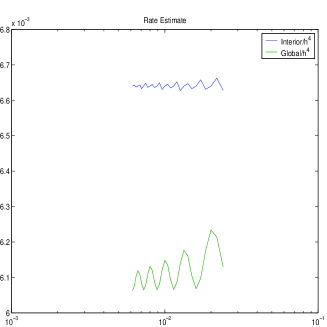
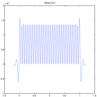
If we use $C=1.2$ and interpolate $f_{2}$ in ${\cal H}(K,\mathbb{R}^{d})$ there. we are in the superconvergence case, because $f_{2}$ is a convolution with $K$ of a function supported in $[-1,+1]\subset\Omega$. The observed rates are around $4$ in $[-1.2,+1.2]$ and in the “interior” domain $[-0.8,+0.8]$, see Figure 1. Up to a Gibbs phenomenon, the interpolant recovers $\chi_{[-1,+1]}$, and this is also visible when looking at the error.

Figure 1: Superconvergence case in $[-1.2,+1.2]$, rate estimates (left) and error function for 41 points (right)

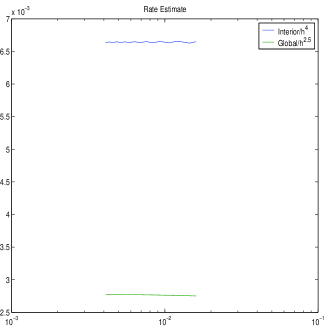
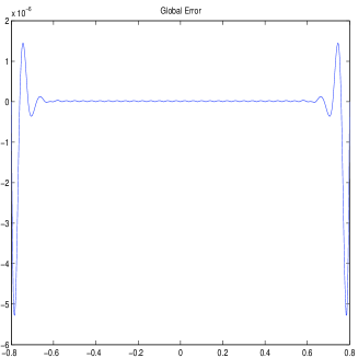
For $C=0.8$, we still have enough smoothness for superconvergence, but the localization condition (7) fails. The standard expected global convergence rate is 2, but in the “interior” $[-0.6,+0.6]$ we still see superconvergence of order 4 in Figure 2. The global error is attained at the boundary.

Figure 2: Convergence in $\Omega:=[-0.8,+0.8]$ and “interior” $[-0.6,+0.6]$, rate estimates (left) and error function for 41 points (right)

Surprisingly, the global rate is 2.5 instead of 2, and this is confirmed for many other cases, even various ones with just $W_{2}^{2}(\mathbb{R}^{1})$ smoothness. This is another instance of superconvergence, and it needs further work. Experimentally, it can be observed that the norms $\|f-s_{f,X,K}\|_{K}$ often go to zero like $1/\sqrt{|X|}$, possibly accounting for the extra $\sqrt{h}$ contribution to the usual convergence rate $2$ that is obtained when assuming that the norms are only bounded by $\|f\|_{K}$.

The standard error analysis of kernel-based interpolation of functions $f\in{\cal H}_{K}(\Omega)$ using a kernel $K$ and a set $X$ of nodes ignores the fact that the Hilbert space error $\|f-s_{f,X,K}\|_{K}$ decreases to zero when $|X|$ gets large and finally “fills” the domain. It seems to be a long-standing problem to turn this obvious fact into a convergence rate that is better than the usual one given by sampling inequalities that just use the upper bound $\|f\|_{K}$ for that error.