Self-Consistent Modeling of Reionization in Cosmological Hydrodynamical Simulations
Abstract
The ultraviolet background (UVB) emitted by quasars and galaxies governs the ionization and thermal state of the intergalactic medium (IGM), regulates the formation of high-redshift galaxies, and is thus a key quantity for modeling cosmic reionization. The vast majority of cosmological hydrodynamical simulations implement the UVB via a set of spatially uniform photoionization and photoheating rates derived from UVB synthesis models. We show that simulations using canonical UVB rates reionize and, perhaps more importantly, spuriously heat the IGM, much earlier than they should. This problem arises because at , where observational constraints are nonexistent, the UVB amplitude is far too high. We introduce a new methodology to remedy this issue, and we generate self-consistent photoionization and photoheating rates to model any chosen reionization history. Following this approach, we run a suite of hydrodynamical simulations of different reionization scenarios and explore the impact of the timing of reionization and its concomitant heat injection on the the thermal state of the IGM. We present a comprehensive study of the pressure smoothing scale of IGM gas, illustrating its dependence on the details of both hydrogen and helium reionization, and argue that it plays a fundamental role in interpreting Lyman- forest statistics and the thermal evolution of the IGM. The premature IGM heating we have uncovered implies that previous work has likely dramatically overestimated the impact of photoionization feedback on galaxy formation, which sets the minimum halo mass able to form stars at high redshifts. We make our new UVB photoionization and photoheating rates publicly available for use in future simulations.
Subject headings:
intergalactic medium — cosmology: early universe — cosmology: large-scale structure of universe — galaxies: formation — galaxies: evolution — methods: numerical1. Introduction
In our current standard model of the universe, hydrogen and helium account for 99% of the baryonic mass density (Planck Collaboration et al. 2015). After the recombination epoch, these elements remain neutral until ultraviolet radiation from star-forming galaxies and active galactic nuclei reionizes them. Therefore, this ultraviolet background (UVB) governs the ionization state of intergalactic gas and plays a key role in its thermal evolution through photoheating. During the reionization of H i and later He ii, ionization fronts propagate supersonically through the intergalactic medium (IGM), impulsively heating gas to K (see, e.g., Abel & Haehnelt 1999; McQuinn 2012; Davies et al. 2016). As the universe evolves, it is well known that the balance between cooling due to Hubble expansion and inverse-Compton scattering of cosmic microwave background (CMB) photons and heating due to the gravitational collapse and photoionization heating give rise to a well-defined temperature-density relationship in the IGM (Hui & Gnedin 1997; McQuinn 2012):
| (1) |
where is the overdensity with respect to the mean and is the temperature at the mean density. Immediately after the reionization of H i () or He ii (), is likely to be around K and (Bolton et al. 2009; McQuinn et al. 2009); at lower redshifts, decreases as the universe expands, while is expected to increase and asymptotically approach a value of (Hui & Gnedin 1997).
Another important physical ingredient to describe the thermal state of the IGM is the gas pressure support. At small scales and high densities, baryons experience pressure forces that prevent them from tracing the collisionless dark matter. This pressure results in an effective 3D smoothing of the baryon distribution relative to the dark matter, at a characteristic scale. known as the Jeans pressure smoothing scale, . In an expanding universe with an evolving thermal state, this scale at a given epoch is expected to depend on the entire thermal history, because fluctuations at earlier times expand or fail to collapse depending on the IGM temperature at that epoch (Gnedin & Hui 1998; Kulkarni et al. 2015). Recently, Rorai et al. (2013) and Rorai et al. (2015) have shown that an independent measurement of the pressure smoothing scale can be obtained using the coherence of Lyman- forest absorption in close quasar pairs (Hennawi et al. 2006, 2010).
Lyman- forest observations between probe the moderate overdensities characteristic of the IGM and therefore are a crucial tool to understand the properties of the UVB. In the last decade, the precision of these measurements has continued to grow both in terms of their numbers (BOSS111Baryon Oscillation Spectroscopic Survey (BOSS): https://www.sdss3.org/surveys/boss.php survey) and in quality (high signal-to-noise ratio spectrum from, e.g. O’Meara et al. 2015). However, while it seems that we keep learning more and more about the ionization history of the universe, for both H i and He ii reionizations (e.g. Becker & Bolton 2013; Syphers & Shull 2014; Worseck et al. 2014; Becker et al. 2015) the thermal history of the universe is still far from certain. The statistical properties of the Lyman- forest are sensitive to the thermal state of the gas, trough both thermal broadening of lines and pressure support. When constraints on the thermal history are reviewed, they yield very puzzling results. Measurements of from different groups utilizing different methodology are in poor agreement (Schaye et al. 2000; Bolton et al. 2008; Lidz et al. 2010; Becker et al. 2011; Rudie et al. 2012; Garzilli et al. 2012; Boera et al. 2014; Bolton et al. 2014). A similar problem appears when measurements of the slope of the temperature–density relation, , are compared. At some authors have even found that is either close to isothermal () or even inverted (; Bolton et al. 2008; Viel et al. 2009, but see Lee et al. 2015). Most studies of the thermal state of the IGM ignore uncertainties resulting from the unknown pressure smoothing scale (but see Becker et al. 2011; Puchwein et al. 2015), which produces a 3D smoothing that is difficult to disentangle from the the similar but 1D smoothing resulting from thermal broadening (Peeples et al. 2010a, b; Rorai et al. 2013). Therefore, ignoring this effect has probably contributed to the confusing and sometimes contradictory published constraints on and (Puchwein et al. 2015).
With the help of accurate models of the IGM, the statistics of the Lyman- forest can be used to constrain its thermal parameters and ultimately cosmic reionization. Ideally one will run coupled radiative transfer hydrodynamical simulations that include extra physics governing the sources of ionizing photons (stars, quasars, etc.). Despite significant progress on this front (Wise et al. 2014; So et al. 2014; Gnedin 2014; Pawlik et al. 2015; Norman et al. 2015; Ocvirk et al. 2015) these simulations are still too costly for sensible exploration of the parameter space. For this reason, the dominant approach, implemented in the vast majority of hydrodynamical codes, is to assume that all gas elements are optically thin to ionizing photons, such that their ionization state can be fully described by a uniform and isotropic UV+X-ray background radiation field. Thus, the radiation field is encapsulated by a set of photoionization and photoheating rates that evolve with redshift for each relevant ion. The minimal set of ions are H i, He i and He ii in order to track the most relevant ionization events, as well as the thermal heating associated with them. Of course, although this optically thin approximation is a valid assumption once the mean free path of ionization photons, , is large enough, it is certainly not true during cosmic reionization events. As such, this optically thin approach is not meant to provide an accurate description of reionization itself, but it should at least provide a reasonable description of the heat injection associated with reionization.
This is important since galaxies forming during the reionization epoch are sensitive to the thermal state of the gas, and even well after reionization gas elements can retain thermal memory of reionization heating (Gnedin & Hui 1998; Kulkarni et al. 2015). It is important to remark here that these UVB models have relevant consequences for galaxy formation and evolution models and hydrodynamical simulations. Several groups have already shown how important the UVB model is to determine the star formation of the first galaxies and their evolution by not only setting the minimum halo mass able to form stars (i.e., halos massive enough to overcome gas pressure forces; Rees 1986; Sobacchi & Mesinger 2013) but also regulating the gas accretion from the IGM into the more massive halos (Quinn et al. 1996; Simpson et al. 2013; Benítez-Llambay et al. 2015; Wheeler et al. 2015).
The standard approach is to adopt photoionization and photoheating rates from semianalytical synthesis models of the UVB (Haardt & Madau 1996, 2001; Faucher-Giguère et al. 2009; Haardt & Madau 2012). However, these UVB synthesis models surely break down during reionization events, and the validity of using them in optically thin simulations (during reionization) is questionable. Moreover, as we will show, these models are fundamentally inconsistent during reionization, leading to different reionization histories in the simulations than the ones given by the authors. Specifically, they reionize the universe too early, and as a result they produce spurious heating of the IGM at early times (see Section 2 and Figure 1). In this paper, we improve on the limitations of current UVB models to provide reliable ionization and thermal histories during reionization by developing a new method to model ionization and heating during reionization in hydrodynamical simulations. In the context of this method, we demonstrate how to run simulations with self-consistent ionization and thermal histories that agree with constraints from the CMB and IGM measurements. Moreover, we make these new tables publicly available in the default format used by most cosmological codes.
The outline of the paper is as follows. In Section 2 we discuss in detail current standard methods that include the effect of the UVB in optically thin hydrodynamical simulations. We show that these models have problems reproducing the desired ionization and thermal histories. In Section 3 we present a new method to improve the current models of the UVB during reionization events. The different reionization models considered in this work, based on current observational constraints, are motivated in Section 4. We describe the basic details of the hydrodynamical cosmological code that we have used in this work, the analysis pipeline, and the properties of the simulations in Section 5. The ionization and thermal histories of the simulations using the new UVB models are shown and examined in Section 6. We explore the possibility of reproducing observational constraints on the H i and He ii transmission in Section 7. In Section 8 we discuss the limitations of our new approach, provide a comparison to previous work, and discuss previous work using incorrect UVB models in galaxy formation simulations that likely overestimate the impact of photoionization feedback. We conclude in Section 9. In Appendix A we provide details on how the new photoionization and photoheating rates are derived in our method. In Appendix B we present the ionization and thermal histories of several widely used UVB models. The effects of cosmology on the new models are discussed in Appendix C. Finally, in Appendix D we present the photoionization and photoheating rates of the new models.
2. Ionization and Thermal Histories of Common UVB Models
Current UVB models used in optically thin hydrodynamical simulations give the evolution of both photoionization, (), and photoheating () rates with redshift. Therefore, during reionizations the simulated IGM is photoheated everywhere by the same spectrum using a homogeneous value of . It is important to remark that the photoheating rates are given as energy per second per ion. Then, for example, in the case of H i reionization, the photoheating rate per volume for each resolution element is .
Haardt & Madau (1996) were the first to try to develop self-consistent UVB models in a cosmological context using radiative transfer methods and taking into account observations of the ionizing sources (namely, quasars and galaxy luminosity functions) and the absorption of the ionizing photons (column density distribution of neutral hydrogen, , absorbers, and H i mean flux). An ionization front heats up the gas behind it (see, e.g., Abel & Haehnelt 1999; McQuinn 2012; Davies et al. 2016) and therefore it is crucial to include radiative transfer effects in the UVB modeling. Self-consistent methods use photoionization modeling codes that implement 1D radiative transfer (e.g. cloudy) to try to take this effect into account. Subsequent efforts have developed these models further (Faucher-Giguère et al. 2009; Haardt & Madau 2012). These UVB models are adopted in essentially all nonadiabatic cosmological hydrodynamic simulations to compute the ionization state and photoheating rates of intergalactic gas (Somerville & Davé 2015). These include simulations focusing on the properties of the IGM (e.g. Katz et al. 1996; Miralda-Escudé et al. 1996; Lukić et al. 2015), but also simulations modeling galaxy formation and evolution (e.g. Vogelsberger et al. 2013; Hopkins et al. 2014; Shen et al. 2014; Governato et al. 2015; Davé et al. 2016).
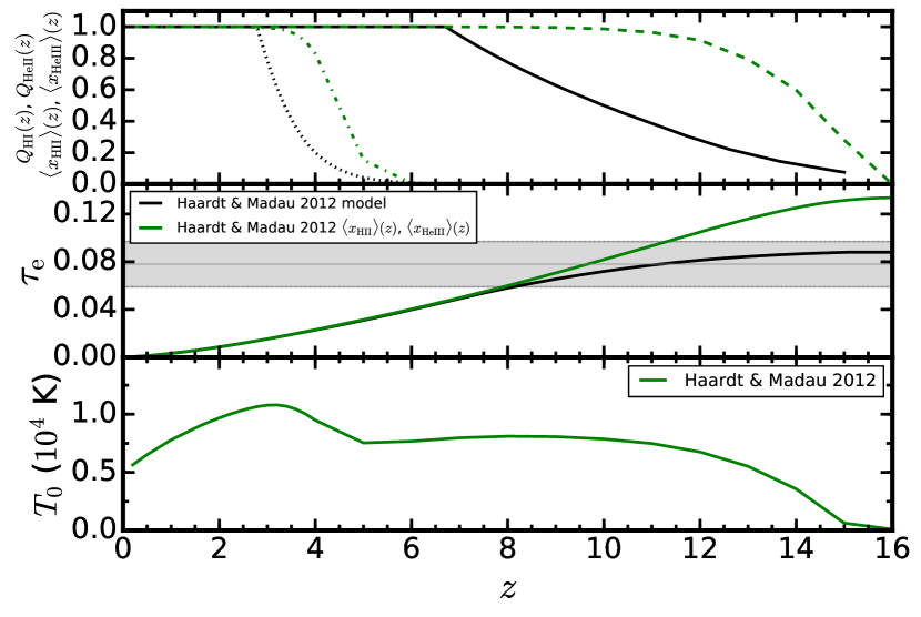
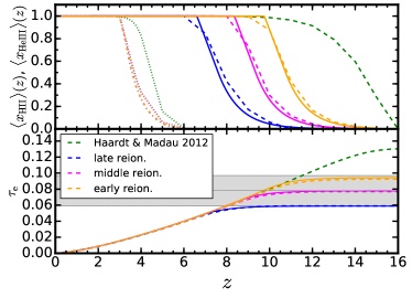
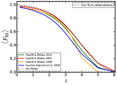
We first want to present the ionization and thermal histories obtained when one of the most widely used UVB models (e.g. tabulated photoionization and photoheating rates) is used (Haardt & Madau 2012, hereafter HM12). The upper panel of Figure 1 shows the H ii (solid black line) and He iii (dot-dashed black line) ionization history calculated by the HM12 model (black lines), which indicates that H i reionization should finish at and He ii at . These are given by the volume filling fraction evolution, which can be thought of the probability that the hydrogen in a given region is ionized (Madau et al. 1999), and the analogous quantity for a doubly ionized helium region. In this panel we also show the ionization history of an hydrodynamical cosmological simulation using the HM12 UVB model (green lines). This simulation uses the standard methodology employed in other optically thin simulations that we describe it in detail in Section 5. To obtain the ionization history from the simulations we computed the ionization fraction of each volume element in the simulation, and , and then calculate the average weighting in volume (i.e. averaging all of the cells)222Notice that calculating the volume filling factor, , is not the optimal way to describe reionization in optically thin simulations. One needs to set up an ionization threshold (standard values are 0.999-0.9) and compute how many cells in the simulation have an ionization fraction above this level. It is easy to see that in optically thin simulations the filling factor evolution will be just a step function that jumps to 1 as soon as the volume-averaged ionization fraction, , reaches the chosen threshold. The temperature evolution shown in Figure 1 illustrates why this approach will not be the correct description of how reionization took place in these simulations.. The first striking thing that we learn from this comparison is that using the HM12 photoionization rates effectively reionizes the universe much earlier than the reionization redshift reported by HM12. It appears that some aspect of the HM12 calculation is not internally consistent.
The middle panel of Figure 1 shows the integrated electron scattering optical depth, defined as
| (2) |
where is the velocity of light, is the Thomson cross section, is the Hubble parameter, and is the proper electron density. We have computed the electron density in our simulation as where and and are the hydrogen and helium mass abundances, respectively (see Appendix A.1 for a detailed derivation of this equation). We also make the standard assumption that the reionization of He i is perfectly coupled with that of H i. The observational constraints on coming from the CMB ( Planck Collaboration et al. 2015) are indicated by a gray band333During the making of this paper, new constraints on reionization from Planck were published (Planck Collaboration et al. 2016), moving these constraints to a lower value and reducing the errors: . These results do no change any of the conclusions of this paper.. The results of the simulation (green) not only differ from the expected results of the model (black) but also they are in strong disagreement with the observational constraints.
Moreover, the lower panel of Figure 1 shows the thermal history of this simulation (green line) via the evolution of the temperature at mean density, defined in eqn. (1). See Section 5.1 for a discussion of the procedure used to fit the - relation. We can see that, not only do reionization events occur too early, but also that the heating associated with them starts at much earlier times, . We have confirmed that this result is not due to resolution, assumed cosmological model, atomic rates considered, or some particular code characteristic (see Figures 3 and A1 in Puchwein et al. 2015, for the same effect but using a SPH Lagrangian code, GADGET-3, and using both an equilibrium and non-equilibrium ionization solver). Thus, why do the reionization histories in the simulation and the one calculated by these authors differ so much?
UVB semianalytic synthesis models — such as the one used by HM12 — rely on two main assumptions: (1) the photoionizing background is everywhere uniform, and (2) radiative transfer is optically thin. Clearly, both assumptions break down during reionization. While a full solution requires a radiative transfer simulation, a large number of IGM studies are insensitive to the reionization details. Thus, the goal is to nevertheless have an approximate UVB background representing the mean UVB to adopt in an optically thin simulation. Therefore, it is important to state upfront that the rates obtained under these sets of assumptions and the ones obtained in a patchy reionization model (e.g., a radiation transfer simulation) can differ significantly during reionization. Lidz et al. (2007) illustrate this point in a simple way by considering two toy models. In the first case, representing patchy reionization, we imagine equal-sized ionized bubbles each with an interior neutral fraction , filling a fraction of the volume of the IGM, which is otherwise completely neutral. For simplicity, we neglect helium and consider an IGM with a uniform density and temperature. In the second model, representing uniform ionization the neutral fraction is identical at each location within the IGM with . In each case, photoionization equilibrium tells us that , where here is the recombination factor. Now, in a uniformly ionized IGM we get . In the toy patchy model, we have inside each ionized bubble and outside of ionized regions. Hence, . The ratio of the volume-averaged photoionization rates is just . This will typically be a very large number: for example, if % of the volume is filled by ionized bubbles each with an interior neutral fraction of , the volume-averaged photoionization rate is a factor of times larger in the patchy reionization model than in the uniform model.
This is also relevant to understanding how the ionization history given by the volume filling factor can be compared with the one given by the volume-averaged ionization fractions and the intrinsic differences between the two. The formalism only knows about sources and sinks of ionizing photons and does not tell us anything about the value of the neutral fraction in highly ionized regions. In what follows we focus on hydrogen reionization, but analogous considerations also apply to helium. The volume filling factor evolution in UVB synthesis models is computed as
| (3) |
where is the hydrogen recombination time and is the mean number of ionizing photons emitted by all radiation sources available per second444The recombination time for H i reionization is generally defined as where is the recombination coefficient to the excited states of hydrogen, accounts also for the presence of photoelectrons from singly ionized helium, and is the clumping factor of ionized hydrogen. A practical issue is how should be evaluated when , and in particular when . We refer to the nice and detailed discussion on this issue done by (So et al. 2014). In any case, recombination rates are relatively unimportant at high redshifts, and this possibility cannot explain the big discrepancy between the model and the simulation.. In the context of these models, , is considered to be the number of ionizing photons emitted into the IGM by all radiation sources (HM12; So et al. 2014) where is the total emissivity as a function of frequency obtained by the assumption of the sources (i.e. galaxies and quasars luminosity functions)555These models also need to assume some galaxy escape fraction at each redshift that is generally chosen by first iteratively solving the integrated cosmological radiative transfer equation This model uses observational constraints of the distribution of absorbers along the line of sight, and it is able to reproduce available measurements of the mean free path at Ryd and the Lyman- effective opacity.
To clarify what is happening at these high redshifts we can use the equation of cosmological radiative transfer in its “source function” approximation, which allows to write the following relation between emissivity, radiation intensity and mean free path, by ignoring photon redshifting effects (minimal at high redshifts): if only local radiation sources contribute to the ionizing background intensity (HM12). From this relation it is now much more easy to see what went wrong in the UVB model. The H i photoionization rates, given by HM12 are calculated as
| (4) |
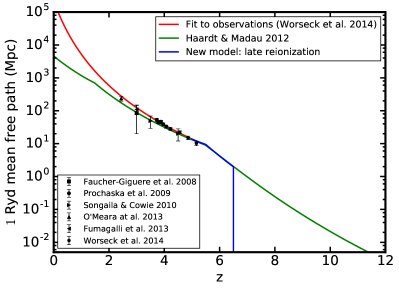
where is the radiation intensity. The ionization history, , was computed using the emissivity alone, using an analytical approximation that does not know anything about the mean free path assumed in the model. On the other hand, the photoionization rates depend on both the emissivity and the mean free path, indicating that the mean free path extrapolation done at high redshift was wrong and yields values that are systematically too high.. To illustrate this, we show in Figure 2 the mean free path assumed in the model (green line) and observational constraints on the mean free path at Ryd (black symbols). Notice that at high redshifts , there are no available constraints and the model thus corresponds to a blind extrapolation.
The H i photoheating rate (energy per time per ion), , given by these models is calculated as
| (5) |
so the photoionization rates are overestimated for the same reason that the photoheating rates are. As noted above, the total heating rate does not depend on the the amplitude of but only on its shape (Theuns et al. 2002b; McQuinn et al. 2009). However, as we argued above, in the standard UVB semianalytic synthesis modeling approach, and are not required to be internally consistent, so in practice the actual heating rate per volume approaches a constant at early times (), whereas it should go to zero. Therefore, the total heat produced during H i and He ii reionization in the simulation was also applied earlier than when it should be.
We have also tested other widely used UVB models in the literature (Haardt & Madau 1996, 2001; Faucher-Giguère et al. 2009, hereafter HM96, HM01, FG09, respectively). We present the full results for these other models in Appendix B showing that they all share a similar problem, i.e., for H i or He ii (or both) reionization the gas heating associated with the reionization event occurs much earlier than one will naively expect from these models. Although it was known that these UVB models do not properly model the reionization process, it is important that this problem has not been directly confronted in the literature (see, however, Puchwein et al. 2015). This oversight is likely due to the fact that, for the ionization and thermal histories of the IGM, most comparisons between simulations and observations have been performed in the context of the Lyman- forest and focused on the redshift range for which such observations are available, i.e. between , or even lower redshifts. The thermal parameters studied so far in the literature, and , depend on the instantaneous values of these rates once we are far enough in time from reionization. So they quickly forget about early heating Therefore, what happens at higher redshifts is not that relevant for these values. However, it is expected that this problem will have more important consequences for correctly modeling the pressure smoothing scale, as it depends on the full thermal history. This is because at IGM densities, the dynamical time that it takes the gas to respond to temperature changes at the Jeans scale (i.e., the sound-crossing time) is the Hubble time (Gnedin & Hui 1998).
To summarize, current UVB models result in different ionization and thermal histories than those quoted by the authors. This is because the low- mean free path values have been blindly extrapolated to high- (see Figure 2), where they result in a photoionization rate far too high. Motivated by these results, we have developed a new method to build self-consistent effective ionization and thermal histories during reionization epochs in optically thin simulations, which we describe in the next section.
3. Improved UVB Models
As stated in the previous section, current photoionization rates widely used in optically thin codes do not properly track the desired ionization histories and lead to incorrect thermal histories for the gas in these simulations, where the gas is heated much earlier than it should be. We present here a new way of creating self-consistent UVB models during reionization events (H i, He i, and He ii) to be used in optically thin hydrodynamical simulations. Different groups in the field have modified these tables, both ionization and photoheating rates (especially photoheating, and more in the context of He ii reionization where more observations are available), with different justifications: accounting for different physical effects as nonequilibrium ionization or radiative transfer effects, matching specific observables, or just exploring the parameter space (e.g., Haehnelt & Steinmetz 1998; Theuns et al. 2002a; Bolton et al. 2005; Jena et al. 2005; Wiersma et al. 2009; Pawlik et al. 2009; Puchwein et al. 2015; Lukić et al. 2015). However, this has generally been done by just applying a multiplying factor to the standard models assumed or by applying different simple cutoffs666Results of simulations using the cutoff approach can be found in Appendix B..
Our approach will be based on building effective values of the photoionization and photoheating rates that can be substituted into the standard optically thin equations to yield the desired results (see FG09 for an early motivation of this approach). The main goal is to make sure that the heating due to reionization in the simulation is consistent with the reionization model itself. To enforce this, we have calculated the volume-averaged values of both the photoionization and photoheating rates that give us the desired ionization and total heat injection for an input reionization model. We give here a global overview of the method and the different assumptions made in our models. We explain in full detail how we derive the photoionization rates in Appendix A.1 and the photoheating rates in Appendix A.2. We will discuss the different caveats and limitations of our model in Section 8.
Each of our reionization models is defined by one free parameter, the total heat input during reionization, and one free function, the reionization history, which in this context we define as the volumen-averaged ionization fraction evolution, . The reionization of He ii is analogously treated. Using these parameters, we will derive effective photoionization and photoheating rates that can be used in hydrodynamical simulations using the following assumptions:
-
1.
That all species are in ionization equilibrium at all times. This is done to be fully consistent with (most of) the codes that will be using these UVB models but it could be changed in the future.
-
2.
That the gas composition can be approximated as primordial. Therefore, the evolution of the number density of electrons, , is given as .
-
3.
That He i reionization is perfectly coupled with H i reionization.
-
4.
That He ii reionization is not relevant during H i reionization and vice versa.
-
5.
That the heating due to reionization is perfectly coupled to the reionization process. Therefore, the heating can be written as a function of the total heat injection and the ionization history, i.e.,
(6)
Finally, the new effective rates are only used during reionization, i.e., while . Once the reionization redshift, defined as when the input ionization history is one, , is reached, we can simply use the photoionization and photoheating rates of common UVB models (in our case HM12).
Let us first focus on how we obtain the new photoionization rates to be applied during reionization. We obtain the new effective photoionization rates by volume averaging the ionization equilibrium equations and using the assumptions enumerated above. In particular, for the H i photoionization rates we get:
| (7) |
where is a volumen-averaged correction factor linked with the well known clumping factor and is the recombination coefficient for which a specific volumen-averaged temperature of the IGM, , has to be assumed. We refer the reader to Appendix A.1 for all the details777Based on the same idea used to derive the photoionization rates, in Appendix A.1.1, we introduce a numerical method to compute the expected volumen-averaged ionization history outcome in optically thin hydrodynamical simulations from a specific mean photoionization rate, . We recommend this approach to be used in the future when generating different UVB tabulated models..
In addition to affecting abundances, photoionization injects energy into the gas when a high-energy () photon transfers more energy to an electron than what is necessary to unbind it from the atom. In order to include this heat transfer to the IGM by the UVB, models also provide photoheating rates that are included in simulations as an effective energy source. The temperature of the IGM is much more affected by this photoheating and different atomic cooling processes than by the gravitational collapse of cosmic structure. These processes are accounted for as a global heating and cooling term that is added to the equation of energy for the gas:
| (8) | ||||
where represents the combined heating and cooling terms,888We have assumed comoving coordinates: , is the comoving baryon density (), comoving pressure (), is the proper peculiar baryonic velocity (), is the modified gravitational potential, and is the total comoving energy (). Refer to Almgren et al. (e.g. 2013) for details. which can be expanded as
| (9) | ||||
where the first three terms represent the photoheating rates of H i, He i and He ii respectively999Photoheating terms in eqn. (9) are written as they are usually defined in hydrodynamical simulations, a photoheating rate, (in units of energy per time per ion) multiplied by the ion density, , of that resolution element. Therefore, the global heating due to reionization will be determined also by the amount of ions present, and we cannot expect a constant temperature increase, independent of density. We will discuss this in detail in Section 8.. We have also included an atomic cooling term () and an inverse-Compton scattering term ().
We can obtain effective photoheating rates for the reionization heating by volume-averaging the relation between the heat per unit of time produced by a certain reionization model, , and the one produced by a photoheating rate. This will allow the use of our new models in standard hydrodynamical codes. For the H i photoheating rate, and using the set of assumptions enumerated above, we obtain
| (10) |
where is the hydrogen mass abundance, is the volumen-averaged molecular weight, the assumed reionization history of the model, is its total heat input, and is a volumen-averaged correction factor that we set to one at all redshifts. We refer the reader to Appendix A.2 for more details on how this equation was obtained.
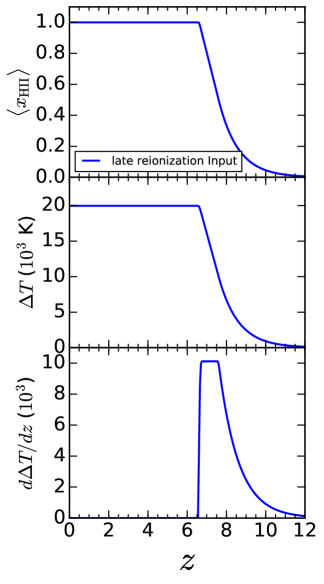
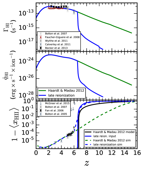
Figure 3 shows an example of how a UVB model is built. In the left panel we show a model that should match a specific late H i reionization history that assumes a reionization redshift of (late reionization model; see more details in Section 4) with a total heat input due to H i reionization of K. The upper left panel shows the H i ionization history assumed to build the model. The middle panel shows the assumed temperature evolution of the H i reionization event. As explained above, we have assumed that the temperature evolution follows the ionization history. The lower left panel shows the actual instantaneous heat input, , derived using eqn. (A19) for this model. The integral of this line gives the total heat input, .
The upper right panel gives the H i photoionization rate (blue line) obtained using eqn. (7) and the method described above. This rate is compared with the equivalent of the HM12 model (green line). We also plot observational constraints on the photoionization rates from different studies (Bolton & Haehnelt 2007; Faucher-Giguère et al. 2008; Wyithe & Bolton 2011; Calverley et al. 2011; Becker & Bolton 2013). Notice that all these constraints are below . The middle right panel shows the photoheating rates derived using eqn. (10) for the H i. Notice that for the new model, below its reionization redshift () we apply the same photoionization and photoheating rates used in HM12 as we think that they are reasonable after reionization. The rates of our model raise abruptly at around the reionization redshift because in the input H i reionization model the transition from to is very fast. The lower right panel shows the reionization function input for the model (solid blue line; defined to be at ). It also shows the volumen-averaged H i ionization fraction obtained running a cosmological hydrodynamical simulation that uses this new photoionization rate (dashed blue line). The solid black line shows the reionization evolution of the HM12 model as calculated by their authors, while the dashed green line stands for the outcome of a hydrodynamical simulation using the HM12 photoionization rate. Current best observational constraints on the H i fraction at different redshifts are also plotted using different symbols and errorbars (Bolton et al. 2005; Fan et al. 2006; Bolton & Haehnelt 2007; McGreer et al. 2015). Notice again that all available constraints are below so that both models are in agreement with these observations.
We can derive the evolution of the mean free path at 1 Rydberg for the new model, making some simple assumptions, and compare it with the ones obtained by HM12. Our modeling has no shape information on the intensity, ; however, one can assume the HM12 shape and that all intensities differ by the same constant: . With this we can approximate the new radiation intensity at 1 Ryd as the ratio between the two photoionization rates . Then we obtain the mean free path using the source function approximation that has the same emissivity assumed by HM12: . Figure 2 shows the evolution of the mean free path derived for this new model (blue line). The green solid line stands for the mean free path used in the HM12 model. This plot illustrates how the volumen-averaged mean free path drops significantly above the reionization redshift.
4. Reionization Models
We will now discuss the different reionization models that we want to simulate by using our new approach to compute photoionization and photoheating during reionization. In order to define a reionization model, we need to set the H i and He ii reionization history via the volumen-averaged ionization fractions101010As eqn. (7) above shows, we also need to define the total heat input expected from each reionization process because there is also a weak dependence on temperature due to the recombination factor..
First, we need to define the shape of our reionization histories. We use the lower incomplete gamma function, :
| (11) |
where , and is a free parameter that sets the redshift where . This function defines a slower start for the reionization function but a fast finish. This specific shape was motivated by radiative transfer simulation results (Ahn et al. 2012; Park et al. 2013; Pawlik et al. 2015) which seem to favor rapid and sudden H i reionization histories in (Mpc/h)3 cosmological volumes. In particular, and were fitted to mimic Pawlik et al. (2015) results. In this work we use only this shape and experiment with the redshift of reionization, but our function could be easily modified in the future to explore a wider range of models. We explore the relevant range of reionization parameters taking into account the CMB constraints on the integrated electron scattering optical depth, (Planck Collaboration et al. 2015)111111In this work we used less constraining results based just on temperature and polarization Planck data. Using more data reduces slightly the best value, but it is still in agreement with this best value. During the making of this paper new constraints on reionization from Planck were published (Planck Collaboration et al. 2016), moving this constraints to a lower value and reducing the errors: . These results do no change any of the conclusions of this paper and in fact emphasize the disagreement between standard UVB models and these observational constraints.. We consider three models: an early, middle, and late H i reionization history, which have reionization redshifts121212We define the reionization redshift of the models at the redshift when of , , and , respectively, all of which give are within of the CMB measurements. These H i reionization models are plotted as solid lines in the upper panel of Figure 4 and their associated values are shown in the lower panel.
For He ii reionization we consider a history based on FG09 (last column of their Table ) results which sets the HeII reionization redshift to finish at (hereafter He_A). The specific evolution of the full ionized fraction can be well described by . This is in agreement with standard models of He ii reionization, which, as a result of the high energy requirement to double ionize helium ( eV), assume that quasars must be the main drivers of this process (e.g., Miralda-Escudé et al. 2000; Compostella et al. 2014; Worseck et al. 2015). This He ii reionization model is plotted as a dot-dashed line in the upper panel of Figure 4.
4.1. Total Heat Input due to H i and He ii Reionization
The other two parameters that define the reionization events in our models are the total heat input that happens during H i and He ii reionizations. There have been several efforts to calculate the specific cumulative energy increase or total heat input (,) due to reionization events. Approximate analytical estimates of this energy can be made given some specific assumptions for the intrinsic spectral slopes of the sources responsible for reionization, and in general neglecting redshifting effects (Efstathiou 1992; Miralda-Escudé & Rees 1994). One-dimensional radiative transfer codes have also been used to obtain a better understanding of the radiative transfer effects on the energy input into the IGM due to the reionization process (e.g. HM96; Abel & Haehnelt 1999). In recent years better radiative transfer codes have been used to study this problem, and current simple analytic models are motivated by by these radiative transfer calculations (Tittley & Meiksin 2007; McQuinn et al. 2009; McQuinn 2012). Most efforts have focused on He ii reionization (Bolton et al. 2004; McQuinn et al. 2009), but the same set of assumptions have also been applied to H i reionization (Bolton et al. 2009). The range of values discussed in these works for H i reionization center around K with up to a factor of two or three difference depending on the exact assumptions. For He ii reionization typical values have been around K with a similar range of uncertainty. In the context of their calculation of self-consistent UVB synthesis models, FG09 computed the total heat input of their model ( K) and its evolution (i.e. ), finding good agreement with the heat input determined from detailed radiative transfer simulations (McQuinn et al. 2009).
We have treated the total heat input of H i and He ii reionization as free parameters in our models and have chosen values based on the aforementioned literature. In particular, for our default models we will use the standard values assumed for both H i and He ii reionization: K and K. We also consider other models with a range of heat input for both H i reionization ( K) and He ii reionization ( K), respectively.
5. Simulations
The simulations used in this work were performed with the Nyx code (Almgren et al. 2013). Nyx follows the evolution of dark matter simulated as self-gravitating Lagrangian particles, and baryons modeled as an ideal gas on a uniform Cartesian grid. The Eulerian gas dynamics equations are solved using a second-order-accurate piecewise parabolic method (PPM) to accurately capture shock waves. We do not make use of adaptive mesh refinement (AMR) capabilities of Nyx in the current work, as the Lyman- forest signal spans nearly the entire simulation domain rather than isolated concentrations of matter, where AMR is more effective. For more details of these numerical methods and scaling behavior tests, see Almgren et al. (2013).
Besides solving for gravity and the Euler equations, we also include the main physical processes fundamental to modeling the Lyman- forest. First, we consider the chemistry of the gas as having a primordial composition with hydrogen and helium mass abundances of , and , respectively. In addition, we include inverse-Compton cooling off the microwave background and keep track of the net loss of thermal energy resulting from atomic collisional processes. We used the updated recombination, collision ionization, dielectric recombination rates, and cooling rates given in Lukić et al. (2015). All cells are assumed to be optically thin, and radiative feedback is accounted for via a spatially uniform but time-varying UVB radiation field given to the code as a list of photoionization and photoheating rates that vary with redshift following the method described in Section 3.
| Sim | |||||
| (K) | (K) | ||||
| HM12 | HM12aafootnotemark: | … | … | … | … |
| FG09 | FG09bbfootnotemark: | … | … | … | … |
| HM01 | HM01ccfootnotemark: | … | … | … | … |
| HM96 | HM96ddfootnotemark: | … | … | … | … |
| LateR | Late reionization | He_A | |||
| MiddleR | Middle reionization | He_A | |||
| EarlyR | Early reionization | He_A | |||
| MiddleR-Hcold | Middle reionization | He_A | |||
| MiddleR-Hwarm | Middle reionization | He_A | |||
| MiddleR-Hhot | Middle reionization | He_A | |||
| MiddleR-noHe | Middle reionization | None | … | ||
| MiddleR-Hecold | Middle reionization | He_A | |||
| MiddleR-Hewarm | Middle reionization | He_A | |||
| MiddleR-Hehot | Middle reionization | He_A |
In order to generate the initial conditions, we have used the music code (Hahn & Abel 2011) and a camb (Lewis et al. 2000; Howlett et al. 2012) transfer function. All simulations started at to be sure that nonlinear evolution is not compromised (see, e.g., Oñorbe et al. 2014, for a detailed discussion on this issue). Unless otherwise stated, all the simulations discussed in this paper assumed a CDM cosmology with the following fundamental parameters: , , , , and . These values are within agreement with last cosmological constraints from the CMB (Planck Collaboration et al. 2015). The choice of hydrogen and helium mass abundances ( and , therefore ) is in agreement with the recent CMB observations and Big Bang nucleosynthesis (Coc et al. 2013). Simulations were run down to , saving 32 snapshots131313For all simulations we saved an snapshot at the following redshifts: , , , , , , , , , , , , , , , , , , , , , , , , , , , , , , , and . from . Unless otherwise stated, all simulations presented here have a box size of length and resolution elements. This dynamical range guarantees that all the different physical parameters analyzed in this paper are converged with enough accuracy ( errors). We will discuss this issue in more detail in Section 8.1.
We first run one simulation using photoionization and photoheating values from the most widely used models (HM96, HM01, FG09 and HM12). We have already presented the reionization and thermal histories of the HM12 model in Section 2 but below we will further explore other properties of this simulation.141414Results of the simulations using HM96, HM01 and FG09 models can be found in Appendix B We also run the three H i reionization histories presented above, an early, middle, and late reionization model (EarlyR, MiddleR and LateR; see above and Figure 4). All of them share the same heat input during H i reionization, K, and He iii reionization model: and K.
In order to study the effect of different total heat input during H i reionization, , we run three more simulations that share all parameters with the H i middle reionization run, MiddleR, but varying this parameter: MiddleR-Hcold ( K), MiddleR-Hwarm ( K) and MiddleR-Hhot ( K). We also explored the effects of different global net heating during He ii reionization by running a set of four more H i middle reionization simulations (MiddleR, ) in which we just changed the heat input during He ii reionization, : MiddleR-noHe (no He ii reionization), MiddleR-Hecold ( K), MiddleR-Hewarm ( K) and MiddleR-Hehot ( K). A summary of all the relevant parameters used in the runs presented in this work is shown in Table 1 along with the naming conventions we have adopted.
5.1. Analysis of the Simulations
Whenever Lyman- forest spectra are created from the simulation, we compute the H i optical depth at a fixed redshift, which can then be easily converted into a transmitted flux fraction, . That is, we do not account for the speed of light when we cast rays in the simulation; we use the gas state at a single cosmic time. The simulated spectra are not meant to look like full Lyman- forest spectra, but just recover the statistics of the flux in a small redshift window. Our calculation of the spectra accounts for Doppler shifts due to bulk flows of the gas, as well as for thermal broadening of the Lyman- line. We refer to Lukić et al. (2015) for specific details of these calculations. This procedure results in the Lyman- flux as a function of wavelength or equivalently time or distance. Following the standard approach, we then rescale the UV background intensity so that the mean flux of all the extracted spectra from the simulation matches the observed mean flux at the respective redshift (see Section 7 for more details on the specific value that we have chosen). We therefore have neglected noise and metal contamination in our skewers so far, but this will not be relevant in this paper.
Using these skewers we have also calculated the curvature flux statistics, , where,
| (12) |
is the first derivative of the flux with respect to the velocity separation between pixels, and is the second derivative. We have done this for each simulation following the method described in Becker et al. (2011)151515i.e., we renormalize the fluxes of each skewer dividing them by its maximum flux value. Then we only used pixels where the renormalized fluxes are in the range ..
We measured the thermal parameters of the simulation at each snapshot by fitting the relation with linear least squares in and , fitting the range and 161616We have tested that changing these thresholds within reasonable IGM densities produce differences just at a few per cent level (see Lukić et al. 2015, for similar conclusions) and in any case it does not affect the conclusions presented in this work. We also found no relevant effects in the main results of this paper if we employed a different fitting approach as the one used in Puchwein et al. (2015)..
To characterize the gas pressure support in all our simulations, we have followed the recent work by Kulkarni et al. (2015) and use the real-space Lyman- flux, . This quantity is defined as , where is the real-space Lyman- optical depth which is identical to the observed Lyman- optical depth except that the convolution integral that accounts for the redshift-space effects of the peculiar velocity field and thermal line broadening has not been included. This field naturally suppresses dense gas, and is thus robust against the poorly understood physics of galaxy formation, revealing pressure smoothing in the diffuse IGM. The 3D power spectrum is accurately described by a simple fitting function with a gaussian cutoff at , which is then defined as the pressure smoothing scale. This statistic has the added advantage that it directly relates to observations of correlated Lyman- forest absorption in close quasar pairs, proposed as a method to measure this scale, and enables one to quantify it in simulations (Rorai et al. 2013, 2015).
6. The Ionization and Thermal History of the IGM
We now present thermal properties of the IGM in LateR, MiddleR, and EarlyR simulations, which only differ in their redshift of H i reionization. We first focus on the the evolution with redshift of the temperature at mean density, , and the slope of the temperature-density relation, . The left panel of Figure 5 shows the evolution of these parameters for the HM12 run (green line). It also shows the thermal history of the LateR (blue), MiddleR (magenta) and EarlyR (orange) simulations. In the upper left panel we plot the evolution of , which exhibits the expected convergence to a value close to after all reionization events for all models, resulting from the balance of photoheating with adiabatic cooling(Hui & Gnedin 1997; McQuinn & Upton Sanderbeck 2016). The larger decrease of during He ii reionization in the EarlyR, MiddleR, and LateR runs seems to indicate a temperature increase more independent of density than in the HM12 run. Puchwein et al. (2015) have also shown that, for a fixed UVB model, using a nonequilibrium approach will tend to create a more pronounced feature (we will further discuss this in Section 8). In our modeling we use equilibrium photoionization; hence, the flattening occurs for different reasons. In fact, this is just because our ionization model injects more heat to the IGM than in the HM12 model. One expects this type of effect during reionization when applying a uniform UVB model through the whole volume, as in that case we are applying a constant temperature increase at each resolution element. At higher initial temperature this corresponds to a lower increase in the logarithm of the temperature, so that the temperature-density relation flattens in log-log space. This effect gets magnified as we increase the amount of heat applied to the whole box. Therefore, our results show that the exact evolution of in simulations depends on the assumed shape for the H i and He ii reionization histories and their total heat input. In this panel we also plot the value of of Bolton et al. (2014) at , derived from absorption-line profiles in the Lyman- forest. 171717We do not directly compare to other measurements of (Ricotti et al. 2000; Schaye et al. 2000; McDonald et al. 2001; Garzilli et al. 2012) because they are either significantly less precise, employ outdated simulations, do not sufficiently treat degeneracies between and , or have other differences in methodology that make direct comparisons between them challenging.
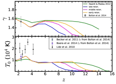
The lower left panel of Figure 5 shows the evolution of for the same set of simulations. As expected, in the new models H i reionization produces a much later heating than in the HM12 run. In fact, it can be clearly seen that the temperature at mean density of the new runs rises following the H i reionization of each model. The heating during He ii reionization also shows significant differences with the HM12 run. Although the heating happens at basically the same time as in the HM12 run, the new models also exhibit a larger and sharper temperature increase at lower redshifts (), along with the expected decrease of the value. This is due to the different ionization history assumed for He ii which rises steeply at these redshifts. We compare these models to the measurements of the temperature at mean density, , from Lidz et al. (2010), based on the wavelet technique (Meiksin 2000; Theuns & Zaroubi 2000). We also plot constraints obtained by combining the measurement by Bolton et al. (2014) plotted in the upper panel with measurements of the temperature at the optimal density, , by Becker et al. (2011) and Boera et al. (2014) derived from the observed curvature of the Lyman- forest transmitted flux. In this case we propagated errors from both measurements. Since observations of the Lyman- forest are only available at , Figure 5 illustrates that it will be challenging to constrain H i reionization from measurements of and at these redshifts because the IGM quickly loses thermal memory of HI reionization. Our new UVB models provide, by construction, a sharper temperature rise due to He ii reionization than the HM12 run. This again illustrates that the exact evolution of the IGM thermal parameters depends on the the assumed shape for the H i and He ii reionization histories, as well as their total heat input.
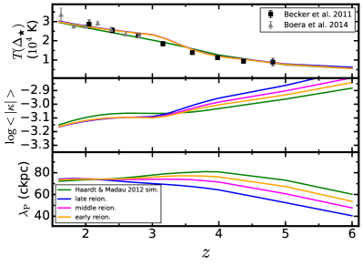
In the upper right panel of Figure 5 we plot another interesting property defining the thermal state of the IGM, which is the temperature at the optimal overdensity, . This “optimal” overdensity at each redshift is defined as the one for which curvature measurements of the Lyman- forest are more sensitive (see Becker et al. 2011; Boera et al. 2014). The curvature measurements allow one to determine this parameter because they are not able to break the degeneracy between and . To calculate the of our simulations, we have used the function fit to these optimal densities by Becker et al. (2011) from a suite of hydrodynamical simulations ( where and )181818Using optimal densities given by Boera et al. (2014, and ) does not change any of the conclusions of this paper.. Inspecting Figure 5, we see that all simulations give the same temperature at the optimal density at , which is not surprising as we have already shown that at these redshifts all of them have roughly the same temperature-density relation (see the left panel of Figure 5). We also see the more pronounced rise in temperature due to He ii reionization in the new models compared with HM12 between .
The middle right panel of Figure 5 shows the curvature flux statistics, , for all these simulations, and it is clear that they do not match at these redshifts. This is because, as explained above, the flux statistics depends not only on the temperature density relation of the IGM (, ), but also on the pressure smoothing scale of the IGM, . In fact, the lower right panel of Figure 5 shows the evolution of the pressure smoothing scale, , with redshift for all the simulations. This panel clearly illustrates the dependence of the pressure smoothing scale on the full thermal history of the universe and not just on the instantaneous temperatures. That is, whereas the temperatures of all models agree at , differences in the pressure smoothing scale persist to much lower redshifts. This explains the differences between the curvature statistics for all the simulations and indicates that for fixed values of and , the value of the optimal density, , will be degenerate with the pressure smoothing scale, .
We have confirmed this by recreating the same study done by Becker et al. (2011) to obtain the optimal densities using hydrodynamical simulations. With a similar set of simulations to that of these authors, we found almost identical results for the values of the optimal densities191919This grid of simulations was created by modifying HM12 heating rates using two factors, and : . However, by including simulations that have identical values of and but different values of , complicates the simple unique definition of by Becker et al. (2011), and instead adds scatter to the relationship between curvature and . The upper panel of Figure 5 also shows the determinations of the temperature at the optimal density using the curvature of the Lyman- forest transmitted flux (Becker et al. 2011; Boera et al. 2014) compared with our simulations. Given the strong dependence of the curvature on the pressure smoothing scale resulting from the different reionization histories, it is clear that the error bars on are likely underestimated. These issues pertaining to the thermal history are discussed in Becker et al. (2011, see also ) but were not included in the error budget. The difference in between our late reionization model (LateR) and early reionization model (EarlyR) at is . From the results presented by Becker et al. (2011, Figure 1 and 10) this difference implies already error in temperature.
The aforementioned issues related to the pressure smoothing scale and thermal history can ease the level of disagreement between Lidz et al. (2010) measurements of and the Becker et al. (2011) measurements of at (Figure 5) although this does not seem to be enough to explain it fully. At lower redshifts a comparison of the two measurements is more challenging because it depends on what one assumes for the the temperature density relation slope, . Based on our results, it is clear that these conflicting measurements lead to different interpretations of the H i and He ii reionization events. On the one hand, the Becker et al. (2011) results point toward a temperature of the IGM at mean density of K by , and a clear heating event later at , which they associated with He ii reionization. On the other hand, Lidz et al. (2010) higher measured temperatures require a higher energy injection () than we assumed in our models ( K) and an earlier injection of heat that could be associated with He ii reionization at higher redshift than inferred by Becker et al. (2011) and Boera et al. (2014). Based on their measurements, Lidz et al. (2010) claim that the He ii reionization event should be completed by and that the temperature at lower redshifts is consistent with the fall-off expected from adiabatic cooling. Although one can argue about the statistical significance of these discrepancies, especially given that the error bars are underestimated because neither study marginalized out the pressure smoothing scale , we see no reason to prefer one set of measurements over the other. For this reason we will not attempt any further interpretation of these measurements with our numerical simulations, and we defer detailed data-to-model comparisons to future work.
We now want to discuss the evolution of the pressure smoothing scale in the different simulations, which, as can clearly be seen from Figure 5, retains memory of the reionization events. As we mentioned in the introduction, this is because, at IGM densities, the dynamical time that it takes the gas to respond to temperature changes at the Jeans scale (i.e., the sound-crossing time) is the Hubble time. The first thing to notice is that the HM12 model results in a much larger pressure smoothing scale than that of any our models, even the early reionization one. This is a direct result of the premature reionization of HI and the spurious associated heating (starting at ) produced by this model. Our new models correct this issue, properly tying reionization heating to reionization history, resulting in later heating and a smaller overall pressure scale. In addition, significant differences are also found below among the simulations with different H i reionization histories (LateR, MiddleR and EarlyR) even though these simulations share exactly the same photoionization and photoheating values at these redshifts and therefore have very similar thermal parameters, i.e. , , . These differences in arise because the IGM has had more time to respond to its hotter temperature when reionization occurs earlier, resulting in a larger pressure scale. The sensitivity of the pressure smoothing scale to the reionization history highlights the importance of constructing self-consistent models of reionization and applying them to optically thin simulations to better understand the thermal evolution of the IGM.
It is interesting to discuss the redshift evolution that we find for the pressure smoothing scale, using . This parameter can be seen as the gas pressure scale at the density most sensitive for Lyman- observations. Therefore, there are two physical effects that contribute to the value of this parameter. First, the IGM is heated as the universe evolves, so we expect the pressure smoothing scale to increase with time. On the other hand, there is not just one pressure smoothing scale in the IGM, but one for each density and, just from linear theory, we expect it to be higher at lower densities, (Schaye 2001). As we go to lower redshifts, the neutral hydrogen density is being further diluted by the expansion of the universe, and observations start to be more sensitive to higher densities that have a smaller pressure smoothing scale. The combination of both processes can produce the somewhat surprising behavior of flattening of at (decrease in the case of the HM12 model due to an He ii reionization with a lower heat injection). We also found that since all these models share the same UVB after reionization, they tend to converge to the same values at lower redshifts. Although the pressure smoothing scale of the IGM depends on the full thermal history, the thermal memory of past reionization events eventually fades as the gas evolves toward lower redshifts.
6.1. Heating during Hydrogen Reionization
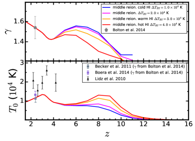
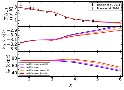
Figure 6 shows the results from simulations (MiddleR-Hcold, MiddleR, MiddleR-Hwarm and MiddleR-Hhot) using different total input heat during H i reionization, i.e., different (, , and K, respectively). All these simulations share the same H i ionization history (middle reionization, ) and exactly the same He ii ionization history and heating. The left panel of Figure 6 shows the evolution of and for these simulations. As expected, they differ significantly during H i reionization, due to the different heat input applied in them. At lower redshifts, , all these simulations share the same HM12 photoionization and photoheating rates; hence, eventually and thermal parameters tend to converge to the same values. This shows again that these thermal parameters depend more strongly on the instantaneous value of these rates. However, it is very interesting to remark that this convergence is not immediate, but that it takes some time for each simulation to converge after reaching the redshift at which they all have exactly the same rates (McQuinn & Upton Sanderbeck 2016). In any case, our simulations show that and have little sensitivity to the details of H i reionization after .
In the right panels of Figure 6 we show the evolution of the temperature at optimal density (, upper panel), the curvature (, middle panel), and the pressure smoothing scale (, lower panel). As expected, , follows the same trend as and (see discussion above). However, the curvature statistics and the pressure smoothing scale for these simulations clearly show a different behavior at redshifts above , while , and have already forgotten reionization at . Simulations with a higher heat input at high redshift show higher pressure smoothing scale values even at lower redshift, due to the dependence of this parameter on the full thermal history. Comparing this result with Figure 5 we can see that the ionization history and the total heat input are degenerate in terms of the pressure smoothing scale. That is, the earlier that H i reionization injects heat into the IGM, the larger the gas pressure scale, . However, a later but hotter (larger heat input) H i reionization also results in a larger pressure smoothing scale. This cautions one about the interpretation of curvature-based measurements of the IGM temperature (Becker et al. 2011) at , since the middle right panel of Figure 6 clearly illustrates that the curvature has a strong dependence on thermal history, even when the instantaneous temperature is the same in all models.
6.2. Heating during Helium Reionization
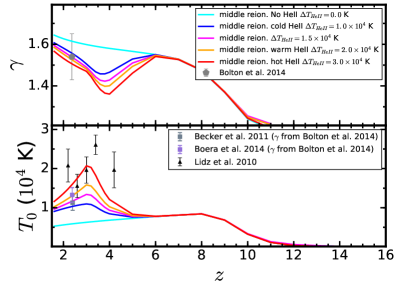
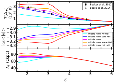
Finally, we discuss simulations for which we modified only the total heat input during He ii reionization. These are MiddleR-noHe, MiddleR-Hecold, MiddleR, MiddleR-Hewarm, MiddleR-Hehot, and the specific values of used in them were (no He ii reionization), , , , and K, respectively. Apart from this, these simulations share exactly the same He i ionization history and also the same H i ionization and photoheating rates (middle reionization, ). Therefore, it is not surprising that the evolution of , , and thermal parameters at redshift above is exactly the same for all simulations (see upper left, lower left, and upper right panels of Figure 7). It is only when He ii reionization starts heating the IGM that these simulations differ. In particular, runs with a higher total heat input result in a much steeper rise when He ii reionization commences in , accompanied by a commensurate fall when He ii reionization is completed. With the slope of the temperature-density relation, , the effect is the opposite. The curvature statistic and the pressure smoothing scale also illustrate the effect of the different heating during He ii reionization. Simulations with a larger late heat input due to He ii reionization give rise to a larger pressure smoothing scale. Notice that the pressure smoothing scales of these models begin to diverge at , once He ii reionization has already completed, as there is a delay before the effect propagates. This delay is due to the dynamical time that it takes the gas to respond to temperature changes at the Jeans scale (i.e., the sound crossing time), which, as discussed above for IGM densities, is close to the Hubble time.
7. Calibrating the UVB to Yield the Correct Mean Flux
The simplest possible Lyman- flux statistic is the mean transmitted flux , or equivalently, the effective optical depth . It is commonly the case that simulations do not recover the observed mean flux, but that simulated fluxes are rescaled to match the observed mean. This rescaling is often understood as equivalent to adjusting the specific intensity of the H i photoionization rate used in the simulation and is justified based on how poorly constrained the ionizing background is. Notice, however, that this rescaling is generally done directly in redshift space. Lukić et al. (2015) conducted a detailed study of the effect that this rescaling can have on different Lyman- statistics. They found that for the large rescalings — those where optical depth has to be rescaled by a factor of 2 or more — the error on flux power spectrum is a few percent. Also, the larger the rescaling is, the larger the error that is introduced. The rescaling error is therefore small, but not negligible, and most importantly, it is puzzling why one should continue to run simulations that systematically produce mean flux values excluded by observations at the few sigma level, and continue to compensate by rescaling the optical depth by a factor of few as is currently required with the HM12 or FG09 UVB tables. For this reason we wish to correct for this error in our new UVB models by renormalizing the input H i photoionization rate so that the post-processing correction will be minimal at all relevant redshifts. We want to emphasize here that the goal of this step is not to remove the need for future rescaling of the optical depth in simulations, but only to ensure that mean fluxes obtained by simulations are roughly consistent with current observations, therefore removing the need for large rescalings. Trying to do better than that would be pointless exercise, as the change in cosmological parameters, as well as having different resolution or box size, will anyway change the mean flux at a few percent level. The resolution of the simulations discussed here is thus sufficient for obtaining mean flux converged at a few percent level (Lukić et al. 2015). In fact, we have run simulations of our LateR, MiddleR and EarlyR UVB models using a larger box size, and resolution elements to confirm that this is indeed the case.
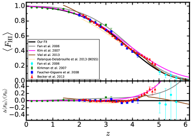
Observational constraints coming from quasar absorption lines (Fan et al. 2006; Becker et al. 2007; Kirkman et al. 2007; Faucher-Giguère et al. 2008; Becker & Bolton 2013) show that the mean flux smoothly evolves from about at , to about at , as expansion gradually lowers the density and the UVB intensity slowly increases. Figure 8 shows a compilation of these observations using different symbols with error bars. We also plot suggested fits to the mean flux evolution by various authors (Fan et al. 2006; Kim et al. 2007; Viel et al. 2013a). However, none of these fits do a particularly good job of describing the full evolution of the mean flux, and we therefore opt for our own fit using all observational data points between . We found that the functional form
| (13) |
provides an optimal fit, with and as the best-fit parameters. This fit is also shown in Figure 8 as a solid black line.
The left panel of Figure 9 shows the H i mean flux evolution in simulations using different well-known UVB models. It is clear that several of them significantly underpredict the observed mean flux at all redshifts. It is also worth pointing out that, somewhat coincidentally, the HM01 UVB model is doing a good job in recovering the observed mean flux. Notice, however, that since our thermal history is different from theirs, we cannot just assume their photoionization rates. Hence, we have modified the H i photoionization rate in our models after reionization so that the H i mean flux in the simulations matches the fit to current observational constraints. Before H i reionization, when we apply our new methodology, this does not apply. We also modified the H i and He i photoheating rate by the same factor so that the heat input at these redshifts is conserved, i.e., and therefore we get exactly the same thermal histories. We have confirmed that this is the case by comparing the evolution of the thermal parameters in the new models versus the old ones, and we show the mean flux evolution of the MiddleR simulation as a dashed line in Figure 9.
Regarding the effect of changing the thermal history, we have compared the differences between the simulations in which we change the heat input due to He ii reionization. We found differences in the H i mean flux up to and between our our fiducial MiddleR model and the two most extreme simulations MiddleR-Hehot and MiddleR-noHe, respectively. This is because through the recombination factor () the neutral fraction has a sensitivity to the gas temperature, not just the photoionization: . This maximum difference corresponds to , the redshift at which the thermal parameters between these simulations are most different. Of course, simulations using thermal histories that deviate even further from these would increase these differences. We have confirmed that mean flux differences due to current uncertainties in the cosmological parameters have a much weaker effect on the mean flux than any of the above systematics in the UVB models described above (see Appendix C for a full discussion on cosmological parameters).
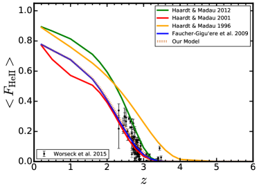
Finally, in the right panel of Figure 9 we show the most recent observations of the He ii transmission (Worseck et al. 2015) and compare them again with the mean HeII flux derived from our hydrodynamical simulations using standard UVB models (HM96, HM01, FG09, HM12)202020Note that in this plot observations compute the mean flux averaging over a much smaller window than in the simulations; however this would only change the variance, but not the mean.. We show the mean fluxes, , and not the optical depths in order to focus on the low redshift results, , where observations seem to indicate that He ii reionization has already finished. Results at higher redshifts are not that conclusive and may indicate that this reionization happened much more slowly than has been assumed (see Worseck et al. 2015, for a detailed discussion). Therefore, we want to focus here just on the low redshift values, where reionization is completed and our method should be valid. For these it seems that FG09 He ii photoionization rates are doing the best job in reproducing the observations. For this reason we decided to use the He ii photoionization and photoheating rates of this model in our new UVB models after He ii reionization.
8. Discussion
In this section we elaborate on the convergence of the results presented in this work, we compare them with recent efforts done in the field, and finally discuss their implications for galaxy formation simulations.
8.1. Resolution and Convergence
We have also run a set of simulations to explore resolution and box size effects on the different methods and parameters discussed in this paper. Some of these results for the mean flux, , and flux power spectrum relevant for this work have already been presented in Lukić et al. (2015). We refer to this work for more details of the accuracy of these simulations. In this regard we are confident that the thermal parameters discussed in this paper, , , and as well as the pressure smoothing scale, , are converged at least at the 5% level for . This is also the case for the curvature statistic, . Although we have used Nyx, an Eulerian code, to run all the tests of the new models created in this work, they will produce the same ionization and thermal histories in any other optically thin hydrodynamical code available. We have explicitly confirmed that Nyx and Gadget (which uses the SPH method for the hydrodynamics) agree well in their values for the mean flux and - relation. Some differences could arise at lower redshifts in some observables, depending on the specific galaxy formation sub-grid model implementation (see e.g., Viel et al. 2013b). However, it is hard to think of a realistic galaxy formation feedback model that will significantly affect the global ionization and thermal histories of the IGM (see, e.g., Kollmeier et al. 2006; Desjacques et al. 2006; Shull et al. 2015, but see Figure 10 of Meiksin et al. 2014).
8.2. Comparison to Previous Work
Recently, Puchwein et al. (2015) tried to solve some of the discrepancies between the HM12 model and observations of thermal parameters by including a nonequilibrium ionization solver in their hydrodynamical simulations. This approach goes in the same direction as this work, in the sense that they both try to improve how things are currently done during reionization events. As was expected, for a fixed UVB model they showed that using a non-equilibrium solver will produce a bigger temperature increase of the IGM during reionization. There is no doubt that a nonequilibrium approach is more physically relevant, as during reionization events the equilibration timescale, which is the time it takes the ionized fraction to change in response to a change in the photoionization rate , can be comparable to the Hubble time, . In a time-dependent (nonequilibrium) ionization calculation the neutral fraction will thus be elevated relative to the equilibrium value, and this results in more photoionization heating, , i.e. is higher in a nonequilibrium calculation. Puchwein et al. (2015) found that this effect brings the HM12 model much more in agreement with the Becker et al. (2011) curvature measurements.
Puchwein et al. (2015) also showed that the change of the slope in the temperature density relation of the IGM, , is in fact significantly smaller in the ionization equilibrium approximation by running the same UVB model using ionization equilibrium and nonequilibrium algorithms. However, the different thermal histories that we found using our new UVB models indicate that this in fact degenerated with the ionization history and total heat input of the reionization event assumed to build the UVB model. The Puchwein et al. (2015) calculations use the HM12 heating rates, which are based on cloudy 1D slab calculations. The validity of the various approximations is dubious, as the heating during reionization is a complicated physical process that depends not only on the shape of the spectrum but also on the local density field and how fast the ionizing front travels (McQuinn 2012; Davies et al. 2016). Due to the present lack of knowledge about how much and when the reionization heats the IGM, we prefer to simply parameterize our ignorance of the details of reionization heat injection with a free parameter . The differences in the IGM thermal properties between equilibrium and nonequilibrium codes thus seem moot given the large uncertainty in this parameter. However, as observational constraints improve and begin to constrain , an improvement of our calculation would be to implement a nonequilibrium calculation along the lines of Puchwein et al. (2015), but from the perspective of our thermal history. This would amount to modification of the value of the that we choose or infer from data. That said, most cosmological hydrodynamical and galaxy formation codes use equilibrium solvers, and thus our current tables have wider applicability in their present assumption of equilibrium.
Recently, Upton Sanderbeck et al. (2015) have also analyzed the thermal histories of different reionization models in a similar spirit as our approach in this work. However, they adopt a fast semianalytical approach that allows them to study how intergalactic gas is heated and cooled during and after reionization processes in a multiple-zone scenario, as opposite to the one-zone model assumption currently used in hydrodynamical simulations. Using this approach, the authors also explored reionization models with different ionization histories and heat injection. This method allows them more freedom in the types of models and parameters that can be explored. It probes to be a very useful tool to build intuition on the possible effects of a wide variety of reionization scenarios. However, a full numerical hydrodynamical method is required to generate simulations of different reionization models that can be directly compared to the observations, and perhaps most importantly, it is not possible to simulate the pressure smoothing effects resulting from different thermal/reionization history analytically. So in fact, the authors must interpret their results on the thermal parameters derived from observations using hydrodynamical simulations.
Finally, we want to point out that both the Puchwein et al. (2015) and Upton Sanderbeck et al. (2015) final conclusions on possible H i reionization scenarios are based only on Becker et al. (2011) measurements at high redshift (), ignoring the constraints on given by Lidz et al. (2010), which point to a much hotter IGM. As discussed above, these two measurements seem to be in disagreement at the 2 level at high redshift, but there is no clear reason to us why any of them should be ignored.
8.3. Implications for Galaxy Formation
As mentioned in the introduction, an ionizing UVB inhibits gas accretion and photoevaporates gas from the shallow potential wells of low-mass dwarf galaxies. This effect due to gas being heated up by photoionization can result in negative feedback: suppressing star formation inside reionized regions, thus impeding their continued growth (see, e.g. Rees 1986; Efstathiou 1992). In our current picture of galaxy formation this feedback is considered to be a good candidate for resolving the ”missing satellite” problem (Moore et al. 1999; Klypin et al. 1999) which arises because in the cold dark matter (CDM) framework the number of simulated dark matter subhalos is much larger than the number of observed dwarf galaxies (Babul & Rees 1992; Bullock et al. 2001). This picture seems consistent with recent observations that have seen uniformly old stellar populations in ultrafaint galaxies (Brown et al. 2014).
This topic has been a very active area of research in the past years, and using cosmological simulations is key to trying to understand these effects in their full context (Quinn et al. 1996; Thoul & Weinberg 1996; Gnedin 2000; Hoeft et al. 2006; McQuinn et al. 2007; Okamoto et al. 2008; Noh & McQuinn 2014; Benítez-Llambay et al. 2015). More recent simulations with much better resolution and a more complete feedback model also seem to point in this direction (Oñorbe et al. 2015; Wheeler et al. 2015). In this context, the work by Simpson et al. (2013) is particularly relevant. Using an enzo high-resolution cosmological hydrodynamical simulation, they found that turning on the UVB at versus resulted in an order-of-magnitude change in the final stellar mass of a dark matter halo. In addition, some very interesting constraints are starting to come from radiative transfer hydrodynamical simulations. Wise et al. (2014) find that very faint galaxies (, in halos of ) will still form at high redshift and contribute a significant amount to the ionizing photon budget during cosmic reionization. However, in order to avoid overproducing the observed abundance of classical satellites of the Milky Way, studies based on dark-matter-only simulations argue for a critical mass closer to (Madau et al. 2008; Boylan-Kolchin et al. 2014).
For all this it is clear that the use of current standard UVB models that reionize and, more importantly here, heat the IGM at a much higher redshift than was desired will have a strong impact on the results of galaxy formation hydrodynamical simulations. For example, simulations that use the HM12 UVB background start spuriously heating up the IGM at (see Figure 1). We can now perform a simple first analytical calculation to get an approximate idea of this effect. In linear theory, the instantaneous cosmological mass cooling threshold of the neutral IGM (sometimes also referred to as the Jeans mass) is given by (see, e.g., Iliev et al. 2007):
| (14) | ||||
where is the temperature of the IGM. As has been found in the simulations mentioned above, the actual cooling mass differs somewhat from this instantaneous Jeans mass since the mass scale on which baryons succeed in collapsing out of the IGM along with the dark matter must be determined, even in linear theory, by integrating the differential equation for perturbation growth over time for the evolving IGM (Gnedin & Hui 1998). In fact, there is no single mass above which a collapsing halo retains all its gas and below which the gas does not collapse with the dark matter. Instead, simulations show that the cooled gas fraction in halos decreases gradually with decreasing halo mass (e.g. Okamoto et al. 2008). Using eqn. (14) can give us a first estimate of the possible effects of using different UVB models. Figure 10 shows the results of this equation when we use the different thermal histories of the HM12, FG09 as well as LateR, MiddleR, and EarlyR models. The differences between the models are quite significant.
Different studies of the reionization redshift of collapse structures have shown that the median reionization redshift of halos moves to lower redshift and the scatter increases (Weinmann et al. 2007; Alvarez et al. 2009; Li et al. 2014). Although both parameters depend substantially on the details of reionization (see, e.g. Ocvirk et al. 2013), massive halos, , can be reionized significantly earlier than the average region in the universe (, see Figure 2 of Li et al. 2014). For Milky Way halos ( , ), or dwarf galaxies ( ) the typical reionization redshift is expected to be much lower ( and respectively), making FG09 and HM12 models not optimal for these studies. This is even more true if one considers the last constraints on from Planck Collaboration et al. (2016). By overestimating the heat at high we are not only overestimating the pressure smoothing scale at lower redshifts but also overestimating the effect of the UVB in galaxy formation and evolution212121Notice that as mentioned above, some authors have tried to solve for this issue by applying different simple redshift cutoffs to the standard UVB models. Results of simulations using the cutoff approach can be found in Appendix B.. For all these reasons, a detailed review of the results of galaxy formation simulations using new consistent UVB models that fulfill all observational constraints, like the ones developed here, is certainly needed. This is another reason why we make the models presented in this work publicly available to the community (see Appendix D) and encourage colleagues to adopt them in future galaxy formation work and revisit previous calculations.
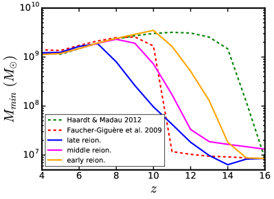
9. Conclusions
In this paper we have presented results from optically thin cosmological hydrodynamical simulations using the Nyx code (Almgren et al. 2013; Lukić et al. 2015). As commonly done in multiple IGM and galaxy formation studies, the UV background is modeled as a uniform and isotropic field that evolves with redshift. Operationally, the UVB determines the photoioinization and photoheating rates of H i, He i and He ii, which are inputs to the code.
We have demonstrated that when canonical models of the UVB, like that of HM12, are used in hydrodynamical simulations, the ionization of the IGM and, more importantly, the concomitant heating occur far too early, inconsistent with the reionization histories calculated by the respective authors, and in violation of current observational constraints on reionization. We argue that this results from the fact that these models dramatically overestimated the mean free path of ionizing photons at root at , resulting from the blind extrapolation of a model fit to lower redshift () measurements. As a result, the amplitudes of the photoionization and photoionization heating rates are far too high at . This premature heating spuriously heats the IGM to K by , and because the IGM gas pressure smoothing scale depends on the full thermal history, it produces an erroneously large pressure smoothing scale at nearly all redshifts. We argue that a correct and consistent model of the reionization and thermal history is crucial for obtaining the correct pressure scale in simulations, which is necessary for interpreting Lyman- forest statistics at – not doing so can bias estimates of the thermal state of the IGM. We also discussed the implications of this spurious early heating on galaxy formation simulations.
Motivated by these issues, we have developed a new method to generate UVB models for hydrodynamical simulations that allow one to self-consistently simulate different reionization models. We implement this by volume-averaging the photoionization and energy equations. In the model, each reionization event is defined by the ionization history with redshift and the total heat input of the reionization event. In this sense our new models provide a very promising tool to explore the parameter space of possible ionization and thermal histories. In this work, we investigated models in which we changed the redshift at which H i reionization ends and the amount of heat input associated with both H i and He ii reionization. We studied the effect of these changes on the thermal history of the IGM, in particular the temperature at mean density, , the slope of the temperature-density relation, , the temperature at the optimal density probed by curvature measurements, , and the gas pressure smoothing scale, . We have shown how important the degeneracies between these parameters can be in order to derive the thermal parameters of the IGM using the curvature Lyman- statistic. These rates have also been corrected to improve the agreement with measurements of the average H i and He ii transmission after reionization.
The UVB plays a fundamental role in determining the star formation of the first galaxies and their evolution by not only setting the minimum halo mass able to form stars but also regulating the gas accretion from the IGM into more massive halos. Previous studies utilizing UVB models that suffer from the spurious early heating described in this paper have thus overestimated the effect of this photoheating feedback and the resulting suppression of star-formation at high redshift. We therefore argue that galaxy formation simulations should be revisited using our new UVB models.
We make our new UVB models publicly available so that the community can better explore the consequences and effects of different ionization and thermal histories in all types of hydrodynamical cosmological simulations. Tables with the photoionization and photoheating rates of the new models can be found in Appendix D, which are in the the standard “TREECOOL” file format, ready and easy to use with most cosmological codes, including gadget, arepo, and gizmo. We encourage anyone interested in implementing some other specific UVB model to contact the authors. We will also be happy to provide help incorporating these models into other codes by request.
Like all optically thin simulations, our approach misses UVB fluctuations that could produce scatter in reionization times and temperatures between different regions of the universe (e.g. Abel & Haehnelt 1999; Meiksin & White 2004; Pontzen 2014; Gontcho A Gontcho et al. 2014; Davies & Furlanetto 2014; Malloy & Lidz 2015; D’Aloisio et al. 2015; Davies & Furlanetto 2016). Of course, an immediate solution to this problem in optically thin simulations will be to add some extra dependence on a specific property of each resolution element in the simulation (e.g. density, distance from a halo that could host a galaxy/quasar, etc). However, the computational challenge is to try to do this without making the simulation prohibitively expensive. In this sense, an interesting solution that it is worth exploring will be to assign a specific reionization redshift to each resolution element of the simulation using, for example, an excursion set formalism (e.g. Furlanetto et al. 2004). In this picture, a resolution element will not see the UVB background until its reionization redshift. We plan to pursue this idea in the near future. Another very valuable piece of information that would improve current optically thin hydrodynamical simulations would be if future radiative transfer simulations (e.g. So et al. 2014; Gnedin 2014; Pawlik et al. 2015; Norman et al. 2015; Ocvirk et al. 2015) were to make the probability distribution function of their photoionization rates publicly available (and perhaps also its dependence on density), and not just the evolution of the mean and/or median values.
Finally, our new parameterization for the heating and ionization produced by the UVB allows us to explore a broader range of reionization models, as well as any other physical scenarios that could alter the thermal history of the IGM. This will allow us to better test the effect of such models in simulations of galaxy formation and the IGM. These models could include Population III stars (Manrique et al. 2015), X-ray pre-heating coming from from starburst galaxies, supernova remnants, or miniquasars (Oh 2001; Glover & Brand 2003; Madau et al. 2004; Furlanetto 2006), dark matter annihilation or decay (Liu et al. 2016) or cosmic rays (Samui et al. 2005), from the intergalactic absorption of blazar TeV photons (Chang et al. 2012; Puchwein et al. 2012), or from broadband intergalactic dust absorption (Inoue & Kamaya 2008). We expect more detailed studies on these physically motivated models in the future.
Appendix A Volume-averaged Ionization and Heating Equations
In this paper we have presented a new way of obtaining effective photoionization and photoheating rates for different reionization models. These can be used in optically thin hydrodynamical simulations to account for emission of the galaxies and quasars. Here we provide detailed derivation of these rates for future reference.
We remind the reader that the new effective rates are only computed during reionization, i.e., while . After reionization, our models use the rates from common UVB models (e.g. FG09, HM12, see Section 7). New values of the photoionization rates during reionization are forced to never exceed the values of the model plugged after reionization. This is done to guarantee no numerical artifacts in the limit where reionization is almost complete, , where our new rates are not well defined.
A.1. Volume Average Optically Thin Ionization Equations
In the context of optically thin hydrodynamical codes, it is often assumed that the gas is of the primordial chemical composition, where the resulting reaction network includes six atomic species: H i, H ii, He i, He ii, He iii and e-. Codes generally evolve those species under the assumption of ionization equilibrium (see, however Gnat & Sternberg 2007; Vasiliev 2011; Oppenheimer & Schaye 2013; Richings et al. 2014a, b; Puchwein et al. 2015, for nonequilibrium treatments). The resulting system of algebraic equations is:
| (A1) | ||||
In addition, there are three closure equations for the conservation of charge and hydrogen and helium abundances. Radiative recombination (), dielectronic recombination (), and collisional ionization () rates are strongly dependent on the temperature, which itself depends on the ionization state through the mean mass per particle
| (A2) |
where is the mass of a proton, is the Boltzmann constant and is the internal thermal energy per mass of the gas. For a gas composed of only hydrogen and helium, is related to the number density of free electrons relative to hydrogen by . The reaction network equations are iteratively solved together with the ideal gas equation of state, , to determine the temperature and equilibrium distribution of species. Above and throughout this paper we have assumed an adiabatic index of .
In order to produce consistent UVB models that reliably reproduce different reionization histories, we have derived the volume-averaged version of the ionization equilibrium equations presented in eqn. (A1). We start with the H i reionization and derive here in detail the equation for H i photoionization. We will address the He single and double reionization afterward, as the method is very similar. We start by doing the volume-averages of eqn. (A1) for H i,
| (A3) |
The first thing is that collisional ionization terms, , are mainly relevant in shocks at high temperatures and densities. They will have a negligible effect on this volume-averaged calculation, so we can discard them. The important point here is that each term in this equation is nonlinear; hence, in principle, it is not possible to compute their volume averages unless the cross-correlation of the abundances of and with each other, as well as with the radiation and temperature fields are known (since and are temperature-dependent). A convenient way to encapsulate this unknown information is using correction factors. With all this we can write the volume-averaged equivalent of eqn. (A1) as
| (A4) |
where the correction factors are defined as
| (A5) | ||||
Then, we can rewrite eqn. (A4) as
| (A6) |
Now, in order to obtain an H i photoionization rate, we will make use of the following assumptions: 1) We assume that the He i reionization occurs perfectly coupled with the H i reionization process. This is a very common assumption in reionization models because ionization of hydrogen and the first ionization of helium require photons with similar energies (13.6 eV and 24.6 eV respectively). Therefore, the same physical process responsible for H i reionization must be also liable for the He i reionization. We also consider that the the helium second ionized state number density is negligible during H i and He i reionization, , so . This is a correct assumption for all the models discussed in this work but could be easily modified in the future if needed. 2) The evolution of number density of free electrons, , can be approximated by . We can rewrite this equation as a function of the hydrogen density and the ionized fractions: where and we have assumed again that He ii reionization follows that of H ii one. The volume-averaged value can be written as
| (A7) |
where factors stand for the correction factors defined as , , etc. As we are assuming that He ii is not relevant during H i reionization, we can discard the second term inside parentheses for our current derivation. Finally, putting together eqn. (A6) with eqn. (A7), we arrive at
| (A8) |
where encapsulates all correction parameters described above and can be written as
| (A9) |
where is defined as to clarify that in general the volume-averaged recombination factor is redefined as the recombination factor at a certain mean temperature value. It is customary to use the temperature at mean density, as this value. In the case of optically thin hydrodynamical simulations a constant photoionization rate is used throughout the whole volume, so .
In general, the unknown ratio of the IGM’s true recombination rate to its hypothetical rate under the assumption of uniform density and temperature is often referred to as the IGM clumping factor (). Notice also that, if for eqn. (A5) we assume that and that is a constant, it is easy to redefine the IGM clumping in a much more familiar form: (Kohler et al. 2007; Pawlik et al. 2009; Finlator et al. 2012; Kaurov & Gnedin 2014).
We can also obtain analogous equations for the volume-averaged helium photoionization rates from eqn. (A1) to the one we obtained above, eqn. (A8), for the hydrogen. We have just made one extra assumption, which is that is negligible during the single reionization of helium and that during the double reionization of helium is negligible. In the context of all the He ii reionization models discussed in this paper this is a fair assumption. For the He first ionization we obtain
| (A10) |
and is analogous to ,
| (A11) |
For the He double ionization,
| (A12) | ||||
In order to describe the reionization history of one model,we will need to specify two functions, the evolution of H ii and He iii volumen-averaged ionization fractions, and . As and and we assume that He i reionization is totally coupled with H i reionization.
To calculate the average values of the radiative recombination rates () which depend on temperature, we need to specify the evolution of the volume-averaged temperature, in our model. To do this, we first need to define the total heat input produced by each reionization event, and which will be two free parameters in our reionization models. We describe in the next paragraph the recent efforts to calculate these parameter from theoretical models. Thus, we will make another assumption in our model to describe the evolution of the volumen-averaged temperature. 3) That the evolution of the volumen-averaged temperature can be well approximated with the evolution of the reionization history times the total heat input, i.e, and . This is a very rough estimation of the thermal history, as we are neglecting all cooling, but it serves as a first-order approximation of the gas temperature during reionization in order to compute the different rates that we need to compute eqn. (A8). We will show below that this assumption is accurate enough for our purposes and for the range of models covered in this work. More elaborate assumptions, including analytic estimations of the Compton cooling, could be implemented in the future.
Finally, to generate the models of this work, we used the following correction factors. For the H i and He i photoionization rates we used for and for . Notice that we never go below redshift when we compute the H i rates, and that these values are in good agreement with results from radiative transfer simulations (clumping factor, , of Pawlik et al. 2009) in this range of redshifts. For the He ii photoionization rates we used at all redshifts, which seems to allow us to accurately recover the input ionization models.
A.1.1 First-order Estimation of the Ionization History in Hydrodynamical Simulations from the Photoionization Rates
Using the relation between volume-averaged quantities derived above, one can obtain an analytical expectation of the volume-averaged H i ionization fraction, , evolution in an optically thin simulations once a certain photoionization rate is assumed. This can be useful to predict the approximate ionization history that a certain photoionization rate model will produce in a optically thin hydrodynamical simulation. In particular, for the H i photoionization rate we can rewrite eqn. (A8) above as
| (A13) |
where now we are using that . If we define , we can rewrite this equation as
| (A14) |
Solving for the volume-averaged H i ionization fraction, we get
| (A15) |
which gives us an estimation of the expected hydrogen neutral fraction once we discard the nonphysical solution. It is expected that changes between simulations that implement very different physical processes. Therefore, this formula could also be used to obtain the value of in optically thin hydrodynamical simulations using one run and then compute analytically the expected results with different UVB models.
A.2. Volume-averaged Heating Equations
The next step is to include in a consistent way the heating occurring during different reionization epochs. To do this, we have implemented a variation of an the idea suggested by FG09.In this work the authors also raised the problems pointed out in the previous section of incorporating the effects of a prescribed UVB in cosmological hydrodynamical simulations under the assumption of an optically thin plasma. Their work was motivated by He ii reionization, but the idea can be well applied for any reionization event. They proposed as a more physically motivated approach to increase the temperature of each gas element by an amount , (which is subsequently allowed to cool) at each time step in the simulation.222222 This method injects the same amount of heat regarding of the density at each resolution element and in fact, we have also implemented it in our code and did several tests. This creates a very different evolution of the temperature-density relation slope, , with redshift. The evolution for the temperature at mean density, , was the same regardless of the method. This method has the advantage of only requiring an additional heating term and adding negligible computational overhead while capturing the timescale and magnitude of the heat input more realistically. Although we might explore it in more detail in the future, we decided to change to our current approach because it implied changing the standard algorithm used in several state-of-the-art cosmological hydrodynamical codes. Our current method produces new UVB models that can be directly plugged into any of these codes. Here is the total heat input or cumulative temperature increase evolution owing to reionization and is precomputed given the desired H i reionization history. Both the total heat input from H i reionization and from He ii reionization will be free parameters in our model. We discuss the specific values used in this work in Section 4.
Now, we want to go one step further from the idea, and relate this change in temperature to a specific photoheating rate, . This will allow the use of our new models in standard hydrodynamical codes. To do this we can, again, volumen-averaged the relation between the heat per unit of time in one cell produced by the model and the one produced by a photoheating rate. The change of internal energy density due to a certain change in temperature of the gas can be related to a new photoheating rate in the following way:
| (A16) |
Using the same assumptions considered to obtain the new photoionization rates, we can get a volume-averaged value for the heating rate. We need also to assume that the volume-averaged molecular weight is . Then we obtain
| (A17) |
where is a correction factor defined as
| (A18) |
Note that this approach sets as we include the heating produced by He i reionization in the H i heating rate. An identical approach is used to obtain the He ii heating rate, . To compute these values in our models, we have used a correction factor, .
Therefore, in our model, once a total heat input due to reionization () is chosen, the exact photoheating rates will depend on the assumption made on . In order to simplify this, we assume that the evolution of the total heat input can be well approximated by the volume-averaged ionization fraction evolution: . From here we can derive the derivative of the total heat input evolution with redshift, which is used in eqn. (A17) to obtain the tabulated photoheating rates that will go into the code. For this reason in our reionization models, the thermal history is defined based on one free parameter, the total heat input , and one free function, the ionization history, which in this context we define as the volumen-averaged ionization fraction evolution, . In the case of H i reionization the heating term is defined as
| (A19) |
The denominator factor is a normalization to guarantee that the integrated amount of heating injected at each time step corresponds to the total heat input.
Appendix B Ionization and Thermal Histories for Other UVB Models
Here we present the ionization and thermal histories produced by other UVB models, widely used in the literature. We have run simulations using the following UVB models (HM96, HM01, FG09), in addition to the HM12 model largely discussed in this work. The left panel of the Figure 12 shows the ionization history for all these models. It is particularly interesting to first focus on the results of the FG09 which use the same approximation as HM12 (Eq. 3) to calculate the reionization redshift of their model that obtained complete He ii reionization by , and H i reionization by . However, it is clear that this model is producing a much higher H i reionization, more close to , indicating that they have the same problems as the HM12 prescription. In fact, the method to compute their expected ionization history is the same as the one used by HM12. In this case the effect is not as extreme, only because tabulated values start at a lower redshift and, although they produce what seems to be a very high redshift H i reionization, the final outcome of the model is still within CMB observational constraints (Planck Collaboration et al. 2015)232323During the making of this paper, new constraints on reionization from Planck were published (Planck Collaboration et al. 2016), moving these constraints to a lower value and reducing the errors: . The HM01 and FG09 models are in clear disagreement at with these new constraints.. We do not have any information on what were the expected ionization histories for the other two older Haardt & Madau models, but it is still very interesting to show their reionization histories, as they are still used in the literature. First of all, notice that in these models, as well as in the FG09 run, the H i reionization is described as a simple step function. The HM01 model assumes a much more shallower He ii reionization history than any other model considered in this work, starting as early as . This will allow us to see the effect of these types of models on the thermal history. HM96 H i reionization happens very late, and therefore this model does not fulfill Planck Collaboration et al. (2015) CMB constraints242424Notice, however, that it is in good agreement with the new Planck Collaboration et al. (2016) constraints..
The middle and right panels of Figure 12 illustrate the thermal histories of these models. The first thing that we want to point out is the effect of a shallower He ii reionization model on the HM01 model. This basically produces a smoother evolution of the temperature at mean density, , eliminating any sharp behavior at lower redshifts. At lower redshifts, the instantaneous thermal parameters and are converging to the same values, but pressure smoothing scale and curvature are not.
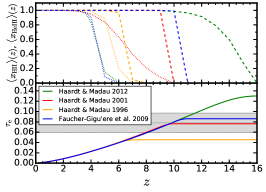
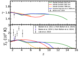
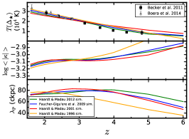
Figure 13 shows results for hydrodynamical simulations in which a simple redshift cutoff was applied to the HM12 model. In this approach the H i and He i UVB rates are set to zero above a certain redshift: (red), (blue), and (brown). We also show the original HM12 model (green lines) for comparison. All the runs share the same He ii rates. The left panel of Figure 13 shows the ionization histories of all these models. The middle and right panels present their thermal histories. As expected, by applying a cutoff to the UVB rates, the reionization redshift and its thermal signatures move down to the cutoff redshift. The gas pressure scale shows very clearly the effect of producing the heating due to H i reionization at lower redshift. As discussed in Section 6, this is because the pressure smoothing scale depends on the full thermal history of the universe and not just on the instantaneous temperatures.
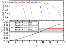
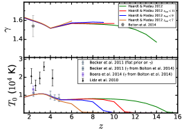
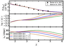
Appendix C Cosmological Effects on the Ionization and Thermal Properties of the IGM
In this appendix we present the results of simulations that only differ in the cosmological parameters and have the same UVB model, HM12. The random seeds in the initial condition are also the same. Table 2 summarizes the cosmological parameters used in each run. Cosmological model A is the default cosmological model used in this work. Models B and C were selected from the posterior distribution of the Planck results (Planck Collaboration et al. 2015) in order to differ as much as possible in the expected matter power spectrum. These should maximize the difference between the models while keeping them within the limits allowed by CMB observations. Model D was used in Lukić et al. (2015) and is also in agreement with the last CMB results.
Figure 14 shows the ionization and thermal histories for these four simulations. Both ionization histories, as well as the evolution of thermal parameters, are almost identical for all the runs. This means that within current observational constraints, the cosmological structure formation does not change significantly the thermal evolution of the IGM, which is determined by the UVB model used. In fact, this result is expected, as from our analytical calculation of the photoionization and photoheating rates we can easily calculate how these rates will change with some cosmological parameters. The difference in photoionization rate values for different cosmologies will be the difference between in the models. Difference in effective photoheating values for different cosmologies will be driven by the difference between 252525In all cases we are assuming the same abundance values for hydrogen, , and helium, ..
We want to emphasize here that even when two simulations/models share the same ionization and thermal evolution, that does not mean that the Lyman- observables (probability density function, flux power spectrum, etc.) from these runs will not show differences between them as the observables could have their own dependence on cosmological parameter or other parameters.
| Model | ||||||
|---|---|---|---|---|---|---|
| A | 0.320 | 0.0496 | 0.681 | 0.670 | 0.826 | 0.966 |
| B | 0.298 | 0.0477 | 0.702 | 0.686 | 0.873 | 0.974 |
| C | 0.333 | 0.0517 | 0.667 | 0.658 | 0.757 | 0.971 |
| D | 0.275 | 0.0460 | 0.725 | 0.702 | 0.816 | 0.960 |
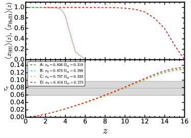

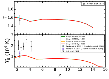
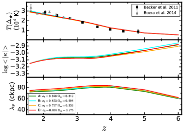
Appendix D New Optically Thin Photoionization and Photoheating Rates
We are making our new UVB models freely available for public use, so that they can be used by the whole community in future hydrodynamical simulations. We provide here the photoionization and photoheating rates for the late H i reionization (table 3), middle H i reionization (table 4), and early H i reionization (table 5) models, assuming a total heat input during reionization of K for H i and K for He ii. The rates for these models are also shown in Figure 15. We refer to Section 3 for a careful explanation on how these rates were obtained. In our new models we have also applied a small correction to the H i and He i photoionization rates of HM12 once reionization is completed to ensure that the simulations match current best observations of the H i mean flux at different redshifts. The goal is to reduce the effect of the current standard post-process rescaling approach done with simulations that aim to reproduce Lyman- statistics. The photoheating rates have been corrected by the same factor in order to keep the heat input per volume element constant in the models and therefore keep exactly the same thermal histories. Section 8 elaborates on the limitations and applicability of these models. Table 3, table 4 and table 5 are published in their entirety in a machine-readable format. Just a portion is shown here, as a guidance to its format and content. We encourage anyone interested in running some other specific model to contact the authors.

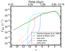
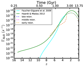
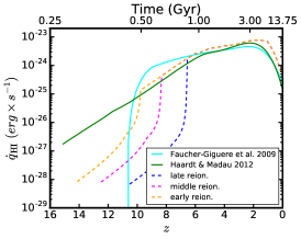
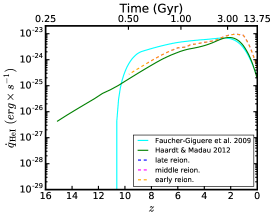
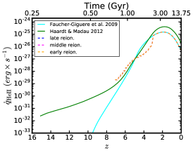
| (s-1) | (s-1) | (s-1) | (erg s-1) | (erg s-1) | (erg s-1) | |
|---|---|---|---|---|---|---|
| 0.0000 | 5.700e-14 | 3.100e-14 | 1.122e-16 | 3.561e-25 | 4.486e-25 | 5.008e-27 |
| 0.0212 | 7.131e-14 | 3.942e-14 | 1.291e-16 | 4.466e-25 | 5.632e-25 | 5.729e-27 |
| 0.0414 | 8.817e-14 | 4.882e-14 | 1.564e-16 | 5.546e-25 | 6.944e-25 | 6.874e-27 |
| 0.0607 | 1.081e-13 | 6.037e-14 | 1.892e-16 | 6.806e-25 | 8.499e-25 | 8.215e-27 |
| … |
| (s-1) | s-1) | (s-1) | (erg s-1) | (erg s-1) | (erg s-1) | |
|---|---|---|---|---|---|---|
| 0.0000 | 5.700e-14 | 3.100e-14 | 1.122e-16 | 3.561e-25 | 4.486e-25 | 5.008e-27 |
| 0.0212 | 7.131e-14 | 3.942e-14 | 1.291e-16 | 4.466e-25 | 5.632e-25 | 5.729e-27 |
| 0.0414 | 8.817e-14 | 4.882e-14 | 1.564e-16 | 5.546e-25 | 6.944e-25 | 6.874e-27 |
| 0.0607 | 1.081e-13 | 6.037e-14 | 1.892e-16 | 6.806e-25 | 8.499e-25 | 8.215e-27 |
| … |
| (s-1) | (s-1) | (s-1) | (erg s-1) | (erg s-1) | (erg s-1) | |
|---|---|---|---|---|---|---|
| 0.0000 | 5.700e-14 | 3.100e-14 | 1.122e-16 | 3.561e-25 | 4.486e-25 | 5.008e-27 |
| 0.0212 | 7.131e-14 | 3.942e-14 | 1.291e-16 | 4.466e-25 | 5.632e-25 | 5.729e-27 |
| 0.0414 | 8.817e-14 | 4.882e-14 | 1.564e-16 | 5.546e-25 | 6.944e-25 | 6.874e-27 |
| 0.0607 | 1.081e-13 | 6.037e-14 | 1.892e-16 | 6.806e-25 | 8.499e-25 | 8.215e-27 |
| … |
References
- Abel & Haehnelt (1999) Abel, T., & Haehnelt, M. G. 1999, ApJ, 520, L13
- Ahn et al. (2012) Ahn, K., Iliev, I. T., Shapiro, P. R., et al. 2012, ApJ, 756, L16
- Almgren et al. (2013) Almgren, A. S., Bell, J. B., Lijewski, M. J., Lukić, Z., & Van Andel, E. 2013, ApJ, 765, 39
- Alvarez et al. (2009) Alvarez, M. A., Busha, M., Abel, T., & Wechsler, R. H. 2009, ApJ, 703, L167
- Babul & Rees (1992) Babul, A., & Rees, M. J. 1992, MNRAS, 255, 346
- Becker & Bolton (2013) Becker, G. D., & Bolton, J. S. 2013, MNRAS, 436, 1023
- Becker et al. (2011) Becker, G. D., Bolton, J. S., Haehnelt, M. G., & Sargent, W. L. W. 2011, MNRAS, 410, 1096
- Becker et al. (2015) Becker, G. D., Bolton, J. S., Madau, P., et al. 2015, MNRAS, 447, 3402
- Becker et al. (2007) Becker, G. D., Rauch, M., & Sargent, W. L. W. 2007, ApJ, 662, 72
- Benítez-Llambay et al. (2015) Benítez-Llambay, A., Navarro, J. F., Abadi, M. G., et al. 2015, MNRAS, 450, 4207
- Boera et al. (2014) Boera, E., Murphy, M. T., Becker, G. D., & Bolton, J. S. 2014, MNRAS, 441, 1916
- Bolton et al. (2004) Bolton, J., Meiksin, A., & White, M. 2004, MNRAS, 348, L43
- Bolton et al. (2014) Bolton, J. S., Becker, G. D., Haehnelt, M. G., & Viel, M. 2014, MNRAS, 438, 2499
- Bolton & Haehnelt (2007) Bolton, J. S., & Haehnelt, M. G. 2007, MNRAS, 382, 325
- Bolton et al. (2005) Bolton, J. S., Haehnelt, M. G., Viel, M., & Springel, V. 2005, MNRAS, 357, 1178
- Bolton et al. (2009) Bolton, J. S., Oh, S. P., & Furlanetto, S. R. 2009, MNRAS, 395, 736
- Bolton et al. (2008) Bolton, J. S., Viel, M., Kim, T.-S., Haehnelt, M. G., & Carswell, R. F. 2008, MNRAS, 386, 1131
- Boylan-Kolchin et al. (2014) Boylan-Kolchin, M., Bullock, J. S., & Garrison-Kimmel, S. 2014, MNRAS, 443, L44
- Brown et al. (2014) Brown, T. M., Tumlinson, J., Geha, M., et al. 2014, ApJ, 796, 91
- Bullock et al. (2001) Bullock, J. S., Dekel, A., Kolatt, T. S., et al. 2001, ApJ, 555, 240
- Calverley et al. (2011) Calverley, A. P., Becker, G. D., Haehnelt, M. G., & Bolton, J. S. 2011, MNRAS, 412, 2543
- Chang et al. (2012) Chang, P., Broderick, A. E., & Pfrommer, C. 2012, ApJ, 752, 23
- Coc et al. (2013) Coc, A., Uzan, J.-P., & Vangioni, E. 2013, ArXiv e-prints, arXiv:1307.6955
- Compostella et al. (2014) Compostella, M., Cantalupo, S., & Porciani, C. 2014, MNRAS, 445, 4186
- D’Aloisio et al. (2015) D’Aloisio, A., McQuinn, M., & Trac, H. 2015, ApJ, 813, L38
- Davé et al. (2016) Davé, R., Thompson, R. J., & Hopkins, P. F. 2016, ArXiv e-prints, arXiv:1604.01418
- Davies & Furlanetto (2014) Davies, F. B., & Furlanetto, S. R. 2014, MNRAS, 437, 1141
- Davies & Furlanetto (2016) —. 2016, MNRAS, 460, 1328
- Davies et al. (2016) Davies, F. B., Furlanetto, S. R., & McQuinn, M. 2016, MNRAS, 457, 3006
- Desjacques et al. (2006) Desjacques, V., Haehnelt, M. G., & Nusser, A. 2006, MNRAS, 367, L74
- Efstathiou (1992) Efstathiou, G. 1992, MNRAS, 256, 43P
- Fan et al. (2006) Fan, X., Strauss, M. A., Becker, R. H., et al. 2006, AJ, 132, 117
- Faucher-Giguère et al. (2009) Faucher-Giguère, C.-A., Lidz, A., Zaldarriaga, M., & Hernquist, L. 2009, ApJ, 703, 1416
- Faucher-Giguère et al. (2008) Faucher-Giguère, C.-A., Prochaska, J. X., Lidz, A., Hernquist, L., & Zaldarriaga, M. 2008, ApJ, 681, 831
- Finlator et al. (2012) Finlator, K., Oh, S. P., Özel, F., & Davé, R. 2012, ArXiv e-prints, arXiv:1209.2489
- Fumagalli et al. (2013) Fumagalli, M., O’Meara, J. M., Prochaska, J. X., & Worseck, G. 2013, ApJ, 775, 78
- Furlanetto (2006) Furlanetto, S. R. 2006, MNRAS, 371, 867
- Furlanetto et al. (2004) Furlanetto, S. R., Zaldarriaga, M., & Hernquist, L. 2004, ApJ, 613, 1
- Garzilli et al. (2012) Garzilli, A., Bolton, J. S., Kim, T.-S., Leach, S., & Viel, M. 2012, MNRAS, 424, 1723
- Glover & Brand (2003) Glover, S. C. O., & Brand, P. W. J. L. 2003, MNRAS, 340, 210
- Gnat & Sternberg (2007) Gnat, O., & Sternberg, A. 2007, ApJS, 168, 213
- Gnedin (2000) Gnedin, N. Y. 2000, ApJ, 542, 535
- Gnedin (2014) —. 2014, ApJ, 793, 29
- Gnedin & Hui (1998) Gnedin, N. Y., & Hui, L. 1998, MNRAS, 296, 44
- Gontcho A Gontcho et al. (2014) Gontcho A Gontcho, S., Miralda-Escudé, J., & Busca, N. G. 2014, MNRAS, 442, 187
- Governato et al. (2015) Governato, F., Weisz, D., Pontzen, A., et al. 2015, MNRAS, 448, 792
- Haardt & Madau (1996) Haardt, F., & Madau, P. 1996, ApJ, 461, 20
- Haardt & Madau (2001) Haardt, F., & Madau, P. 2001, in Clusters of Galaxies and the High Redshift Universe Observed in X-rays, ed. D. M. Neumann & J. T. V. Tran, 64
- Haardt & Madau (2012) —. 2012, ApJ, 746, 125
- Haehnelt & Steinmetz (1998) Haehnelt, M. G., & Steinmetz, M. 1998, MNRAS, 298, L21
- Hahn & Abel (2011) Hahn, O., & Abel, T. 2011, MNRAS, 415, 2101
- Hennawi et al. (2006) Hennawi, J. F., Strauss, M. A., Oguri, M., et al. 2006, AJ, 131, 1
- Hennawi et al. (2010) Hennawi, J. F., Myers, A. D., Shen, Y., et al. 2010, ApJ, 719, 1672
- Hoeft et al. (2006) Hoeft, M., Yepes, G., Gottlöber, S., & Springel, V. 2006, MNRAS, 371, 401
- Hopkins et al. (2014) Hopkins, P. F., Kereš, D., Oñorbe, J., et al. 2014, MNRAS, 445, 581
- Howlett et al. (2012) Howlett, C., Lewis, A., Hall, A., & Challinor, A. 2012, Journal of Cosmology and Astroparticle Physics, 4, 27
- Hui & Gnedin (1997) Hui, L., & Gnedin, N. Y. 1997, MNRAS, 292, 27
- Iliev et al. (2007) Iliev, I. T., Mellema, G., Shapiro, P. R., & Pen, U.-L. 2007, MNRAS, 376, 534
- Inoue & Kamaya (2008) Inoue, A. K., & Kamaya, H. 2008, ArXiv e-prints, arXiv:0810.5614
- Jena et al. (2005) Jena, T., Norman, M. L., Tytler, D., et al. 2005, MNRAS, 361, 70
- Katz et al. (1996) Katz, N., Weinberg, D. H., & Hernquist, L. 1996, ApJS, 105, 19
- Kaurov & Gnedin (2014) Kaurov, A. A., & Gnedin, N. Y. 2014, ApJ, 787, 146
- Kim et al. (2007) Kim, T.-S., Bolton, J. S., Viel, M., Haehnelt, M. G., & Carswell, R. F. 2007, MNRAS, 382, 1657
- Kirkman et al. (2007) Kirkman, D., Tytler, D., Lubin, D., & Charlton, J. 2007, MNRAS, 376, 1227
- Klypin et al. (1999) Klypin, A., Kravtsov, A. V., Valenzuela, O., & Prada, F. 1999, ApJ, 522, 82
- Kohler et al. (2007) Kohler, K., Gnedin, N. Y., & Hamilton, A. J. S. 2007, ApJ, 657, 15
- Kollmeier et al. (2006) Kollmeier, J. A., Miralda-Escudé, J., Cen, R., & Ostriker, J. P. 2006, ApJ, 638, 52
- Kulkarni et al. (2015) Kulkarni, G., Hennawi, J. F., Oñorbe, J., Rorai, A., & Springel, V. 2015, ApJ, 812, 30
- Lee et al. (2015) Lee, K.-G., Hennawi, J. F., Spergel, D. N., et al. 2015, ApJ, 799, 196
- Lewis et al. (2000) Lewis, A., Challinor, A., & Lasenby, A. 2000, ApJ, 538, 473
- Li et al. (2014) Li, T. Y., Alvarez, M. A., Wechsler, R. H., & Abel, T. 2014, ApJ, 785, 134
- Lidz et al. (2010) Lidz, A., Faucher-Giguère, C.-A., Dall’Aglio, A., et al. 2010, ApJ, 718, 199
- Lidz et al. (2007) Lidz, A., McQuinn, M., Zaldarriaga, M., Hernquist, L., & Dutta, S. 2007, ApJ, 670, 39
- Liu et al. (2016) Liu, H., Slatyer, T. R., & Zavala, J. 2016, ArXiv e-prints, arXiv:1604.02457
- Lukić et al. (2015) Lukić, Z., Stark, C. W., Nugent, P., et al. 2015, MNRAS, 446, 3697
- Madau et al. (1999) Madau, P., Haardt, F., & Rees, M. J. 1999, ApJ, 514, 648
- Madau et al. (2008) Madau, P., Kuhlen, M., Diemand, J., et al. 2008, ApJ, 689, L41
- Madau et al. (2004) Madau, P., Rees, M. J., Volonteri, M., Haardt, F., & Oh, S. P. 2004, ApJ, 604, 484
- Malloy & Lidz (2015) Malloy, M., & Lidz, A. 2015, ApJ, 799, 179
- Manrique et al. (2015) Manrique, A., Salvador-Solé, E., Juan, E., et al. 2015, ApJS, 216, 13
- McDonald et al. (2001) McDonald, P., Miralda-Escudé, J., Rauch, M., et al. 2001, ApJ, 562, 52
- McGreer et al. (2015) McGreer, I. D., Mesinger, A., & D’Odorico, V. 2015, MNRAS, 447, 499
- McQuinn (2012) McQuinn, M. 2012, MNRAS, 426, 1349
- McQuinn et al. (2007) McQuinn, M., Lidz, A., Zahn, O., et al. 2007, MNRAS, 377, 1043
- McQuinn et al. (2009) McQuinn, M., Lidz, A., Zaldarriaga, M., et al. 2009, ApJ, 694, 842
- McQuinn & Upton Sanderbeck (2016) McQuinn, M., & Upton Sanderbeck, P. R. 2016, MNRAS, 456, 47
- Meiksin (2000) Meiksin, A. 2000, MNRAS, 314, 566
- Meiksin et al. (2014) Meiksin, A., Bolton, J. S., & Tittley, E. R. 2014, MNRAS, 445, 2462
- Meiksin & White (2004) Meiksin, A., & White, M. 2004, MNRAS, 350, 1107
- Miralda-Escudé et al. (1996) Miralda-Escudé, J., Cen, R., Ostriker, J. P., & Rauch, M. 1996, ApJ, 471, 582
- Miralda-Escudé et al. (2000) Miralda-Escudé, J., Haehnelt, M., & Rees, M. J. 2000, ApJ, 530, 1
- Miralda-Escudé & Rees (1994) Miralda-Escudé, J., & Rees, M. J. 1994, MNRAS, 266, 343
- Moore et al. (1999) Moore, B., Ghigna, S., Governato, F., et al. 1999, ApJ, 524, L19
- Noh & McQuinn (2014) Noh, Y., & McQuinn, M. 2014, MNRAS, 444, 503
- Norman et al. (2015) Norman, M. L., Reynolds, D. R., So, G. C., Harkness, R. P., & Wise, J. H. 2015, ApJS, 216, 16
- Oñorbe et al. (2015) Oñorbe, J., Boylan-Kolchin, M., Bullock, J. S., et al. 2015, MNRAS, 454, 2092
- Oñorbe et al. (2014) Oñorbe, J., Garrison-Kimmel, S., Maller, A. H., et al. 2014, MNRAS, 437, 1894
- Ocvirk et al. (2013) Ocvirk, P., Aubert, D., Chardin, J., et al. 2013, ApJ, 777, 51
- Ocvirk et al. (2015) Ocvirk, P., Gillet, N., Shapiro, P. R., et al. 2015, ArXiv e-prints, arXiv:1511.00011
- Oh (2001) Oh, S. P. 2001, ApJ, 553, 499
- Okamoto et al. (2008) Okamoto, T., Gao, L., & Theuns, T. 2008, MNRAS, 390, 920
- O’Meara et al. (2013) O’Meara, J. M., Prochaska, J. X., Worseck, G., Chen, H.-W., & Madau, P. 2013, ApJ, 765, 137
- O’Meara et al. (2015) O’Meara, J. M., Lehner, N., Howk, J. C., et al. 2015, AJ, 150, 111
- Oppenheimer & Schaye (2013) Oppenheimer, B. D., & Schaye, J. 2013, MNRAS, 434, 1043
- Palanque-Delabrouille et al. (2013) Palanque-Delabrouille, N., Yèche, C., Borde, A., et al. 2013, A&A, 559, A85
- Park et al. (2013) Park, H., Shapiro, P. R., Komatsu, E., et al. 2013, ApJ, 769, 93
- Pawlik et al. (2015) Pawlik, A. H., Schaye, J., & Dalla Vecchia, C. 2015, MNRAS, 451, 1586
- Pawlik et al. (2009) Pawlik, A. H., Schaye, J., & van Scherpenzeel, E. 2009, MNRAS, 394, 1812
- Peeples et al. (2010a) Peeples, M. S., Weinberg, D. H., Davé, R., Fardal, M. A., & Katz, N. 2010a, MNRAS, 404, 1281
- Peeples et al. (2010b) —. 2010b, MNRAS, 404, 1295
- Planck Collaboration et al. (2015) Planck Collaboration, Ade, P. A. R., Aghanim, N., et al. 2015, ArXiv e-prints, arXiv:1502.01589
- Planck Collaboration et al. (2016) Planck Collaboration, Aghanim, N., Ashdown, M., et al. 2016, ArXiv e-prints, arXiv:1605.02985
- Pontzen (2014) Pontzen, A. 2014, Phys. Rev. D, 89, 083010
- Prochaska & Tumlinson (2009) Prochaska, J. X., & Tumlinson, J. 2009, Baryons: What,When and Where?, ed. H. A. Thronson, M. Stiavelli, & A. Tielens, 419
- Puchwein et al. (2015) Puchwein, E., Bolton, J. S., Haehnelt, M. G., et al. 2015, MNRAS, 450, 4081
- Puchwein et al. (2012) Puchwein, E., Pfrommer, C., Springel, V., Broderick, A. E., & Chang, P. 2012, MNRAS, 423, 149
- Quinn et al. (1996) Quinn, T., Katz, N., & Efstathiou, G. 1996, MNRAS, 278, L49
- Rees (1986) Rees, M. J. 1986, MNRAS, 222, 27P
- Richings et al. (2014a) Richings, A. J., Schaye, J., & Oppenheimer, B. D. 2014a, MNRAS, 440, 3349
- Richings et al. (2014b) —. 2014b, MNRAS, 442, 2780
- Ricotti et al. (2000) Ricotti, M., Gnedin, N. Y., & Shull, J. M. 2000, ApJ, 534, 41
- Rorai et al. (2013) Rorai, A., Hennawi, J. F., & White, M. 2013, ApJ, 775, 81
- Rorai et al. (2015) Rorai, A., Hennawi, J. F., White, M., & et al. 2015, in prep.
- Rudie et al. (2012) Rudie, G. C., Steidel, C. C., & Pettini, M. 2012, ApJ, 757, L30
- Samui et al. (2005) Samui, S., Subramanian, K., & Srianand, R. 2005, International Cosmic Ray Conference, 9, 215
- Schaye (2001) Schaye, J. 2001, ApJ, 562, L95
- Schaye et al. (2000) Schaye, J., Theuns, T., Rauch, M., Efstathiou, G., & Sargent, W. L. W. 2000, MNRAS, 318, 817
- Shen et al. (2014) Shen, S., Madau, P., Conroy, C., Governato, F., & Mayer, L. 2014, ApJ, 792, 99
- Shull et al. (2015) Shull, J. M., Moloney, J., Danforth, C. W., & Tilton, E. M. 2015, ApJ, 811, 3
- Simpson et al. (2013) Simpson, C. M., Bryan, G. L., Johnston, K. V., et al. 2013, MNRAS, 432, 1989
- So et al. (2014) So, G. C., Norman, M. L., Reynolds, D. R., & Wise, J. H. 2014, ApJ, 789, 149
- Sobacchi & Mesinger (2013) Sobacchi, E., & Mesinger, A. 2013, MNRAS, 432, 3340
- Somerville & Davé (2015) Somerville, R. S., & Davé, R. 2015, ARA&A, 53, 51
- Songaila & Cowie (2010) Songaila, A., & Cowie, L. L. 2010, ApJ, 721, 1448
- Syphers & Shull (2014) Syphers, D., & Shull, J. M. 2014, ApJ, 784, 42
- Theuns et al. (2002a) Theuns, T., Bernardi, M., Frieman, J., et al. 2002a, ApJ, 574, L111
- Theuns et al. (2002b) Theuns, T., Schaye, J., Zaroubi, S., et al. 2002b, ApJ, 567, L103
- Theuns & Zaroubi (2000) Theuns, T., & Zaroubi, S. 2000, MNRAS, 317, 989
- Thoul & Weinberg (1996) Thoul, A. A., & Weinberg, D. H. 1996, ApJ, 465, 608
- Tittley & Meiksin (2007) Tittley, E. R., & Meiksin, A. 2007, MNRAS, 380, 1369
- Upton Sanderbeck et al. (2015) Upton Sanderbeck, P. R., D’Aloisio, A., & McQuinn, M. J. 2015, ArXiv e-prints, arXiv:1511.05992
- Vasiliev (2011) Vasiliev, E. O. 2011, MNRAS, 414, 3145
- Viel et al. (2013a) Viel, M., Becker, G. D., Bolton, J. S., & Haehnelt, M. G. 2013a, Phys. Rev. D, 88, 043502
- Viel et al. (2009) Viel, M., Bolton, J. S., & Haehnelt, M. G. 2009, MNRAS, 399, L39
- Viel et al. (2013b) Viel, M., Schaye, J., & Booth, C. M. 2013b, MNRAS, 429, 1734
- Vogelsberger et al. (2013) Vogelsberger, M., Genel, S., Sijacki, D., et al. 2013, MNRAS, 436, 3031
- Weinmann et al. (2007) Weinmann, S. M., Macciò, A. V., Iliev, I. T., Mellema, G., & Moore, B. 2007, MNRAS, 381, 367
- Wheeler et al. (2015) Wheeler, C., Oñorbe, J., Bullock, J. S., et al. 2015, MNRAS, 453, 1305
- Wiersma et al. (2009) Wiersma, R. P. C., Schaye, J., Theuns, T., Dalla Vecchia, C., & Tornatore, L. 2009, MNRAS, 399, 574
- Wise et al. (2014) Wise, J. H., Demchenko, V. G., Halicek, M. T., et al. 2014, MNRAS, 442, 2560
- Worseck et al. (2014) Worseck, G., Prochaska, J. X., Hennawi, J. F., & McQuinn, M. 2014, ArXiv e-prints, arXiv:1405.7405
- Worseck et al. (2015) —. 2015, ArXiv e-prints, arXiv:15XX.XXX
- Wyithe & Bolton (2011) Wyithe, J. S. B., & Bolton, J. S. 2011, MNRAS, 412, 1926