Dynamics of Stellar Spin Driven by Planets Undergoing Lidov-Kozai Migration: Paths to Spin-Orbit Misalignment

Abstract

Many exoplanetary systems containing hot Jupiters (HJs) exhibit significant misalignment between the spin axes of the host stars and the orbital angular momentum axes of the planets (“spin-orbit misalignment”). High-eccentricity migration involving Lidov-Kozai oscillations of the planet’s orbit induced by a distant perturber is a possible channel for producing such misaligned HJ systems. Previous works have shown that the dynamical evolution of the stellar spin axis during the high-$e$ migration plays a dominant role in generating the observed spin-orbit misalignment. Numerical studies have also revealed various patterns of the evolution of the stellar spin axis leading to the final misalignment. Here we develop an analytic theory to elucidate the evolution of spin-orbit misalignment during the Lidov-Kozai migration of planets in stellar binaries. Secular spin-orbit resonances play a key role in the misalignment evolution. We include the effects of short-range forces and tidal dissipation, and categorize the different possible paths to spin-orbit misalignment as a function of various physical parameters (e.g. planet mass and stellar rotation period). We identify five distinct spin-orbit evolution paths and outcomes, only two of which are capable of producing retrograde orbits. We show that these paths to misalignment and the outcomes depend only on two dimensionless parameters, which compare the stellar spin precession frequency with the rate of change of the planet’s orbital axis, and the Lidov-Kozai oscillation frequency. Our analysis reveals a number of novel phenomena for the stellar spin evolution, ranging from bifurcation, adiabatic advection, to fully chaotic evolution of spin-orbit angles.

1 Introduction

The discovery of the misalignment between the orbital axes of hot Jupiters (HJs; giant planets with orbital periods of $\sim 3$ days) and the spin axes of their host stars (e.g. Hebrard et al. 2008, 2010; Narita et al. 2009; Triaud et al. 2010; Winn et al. 2009; Albrecht et al. 2012; Winn & Fabrycky 2015) continues to pose a significant puzzle. While primordial disk misalignment (with respect to the stellar spin) is a possible explanation (e.g. Bate et al. 2010; Lai et al. 2011; Foucart & Lai 2011; Batygin 2012; Batygin & Adams 2013; Lai 2014; Spalding & Batygin 2014), it is likely that a significant fraction of HJs and the associated spin-orbit misalignments are produced by dynamical means involving multi-planet interactions or planet-binary interactions.

Lidov-Kozai (LK) oscillations (Lidov 1962, Kozai 1962) induced by external stellar or planetary companions – one of the proposed channels of hot Jupiter formation (e.g. Wu & Murray 2003; Fabrycky & Tremaine 2007; Correia et al 2011; Beaugé & Nesvorný 2012; Naoz et al. 2012; Petrovich 2015; Anderson, Storch & Lai 2016; Muñoz, Lai & Liu 2016; Petrovich & Tremaine 2016) – provide a natural means of generating spin-orbit misalignment. Lidov-Kozai oscillations occur when the proto-HJ’s host star has a binary (or external planetary) companion. A proto-HJ is assumed to form at several AUs from its host. If its orbital axis is sufficiently misaligned relative to the outer binary axis, its orbit undergoes large correlated variations in eccentricity and inclination. If the misalignment is substantial, very high eccentricities (in excess of $0.95$) can be attained; during these high-eccentricity phases, tidal dissipation at periastron brings the planet close to its host, eventually creating a HJ.

Since the host star of a giant planet generally has an appreciable rotation (with rotation period ranging from a few days to 30 days) and is oblate, significant coupling can exist between the orbital dynamics of the proto-HJ and the dynamics of the stellar spin axis. This coupling is vital in determining the final spin-orbit misalignments of these systems. Indeed, in Storch, Anderson & Lai (2014; hereafter SAL14) we showed that the evolution of the stellar spin axis, driven by the quasi-periodic changes in the planet orbit, can be very complex and even chaotic, and this evolution depends sensitively on the planet mass and stellar rotation period. Subsequently, in Storch & Lai (2015; hereafter SL15), we studied the origin of the chaotic behavior (in terms of secular spin-orbit resonances and their overlaps) by analysing the non-dissipative (i.e. no tidal dissipation) “stellar spin + planet + binary” system and considering the regime in which the stellar spin precession rate was much higher than the LK oscillation frequency (the “adiabatic” regime). In Anderson, Storch & Lai (2016; hereafter ASL16), we conducted a comprehensive population synthesis study of HJ formation via LK migration in stellar binaries, including all relevant physical effects (the octupole potential from the binary companion, various short-range forces, tidal dissipation, and stellar spin-down due to magnetic braking). In particular, our extensive Monte-Carlo experiments (see Section 4 of ASL16) revealed various paths of spin-orbit evolution during LK migration.

In the present work, we develop an analytic theory to understand the evolution of spin-orbit misalignment during LK migration in stellar binaries. We extend the analysis of SL15 to the non-adiabatic regime (i.e. the regime in which the star precesses slowly). We account for various non-ideal effects (such as periastron advance due to General Relativity and planet oblateness) and include tidal dissipation in our “stellar spin + planet + binary” system. Our goal is to provide theoretical explanations for the various paths to spin-orbit misalignment that LK oscillations can induce and to shed light on how the final spin-orbit misalignments of HJs are achieved during LK migration. Although our focus is on stellar binary-induced LK migration, most of our results can be adapted to the planet-induced LK migration scenario.

This paper is organized as follows. In Section 2, we briefly review our previous work and introduce the most important concepts and equations in LK-driven spin-orbit dynamics. In Section 3, we discuss the effect that short-range forces have on the spin-orbit dynamics. In Section 4, we examine the different regimes of non-dissipative spin dynamics. In Sections 5 and 6, we include tidal dissipation and study the various paths toward misalignment during LK migration. We identify the key paremeters that determine different behaviors of the misalignment evolution. We discuss the limitations and uncertainties of our work in Section 7 and summarize our key findings in Section 8.

Readers who are less interested in the technical details can go to Section 5.1 for a description of the five different spin-orbit evolution paths (with more detailed explanations in Sections 5.2-5.6), and Section 8 for a brief summary.

2 Lidov-Kozai-Driven Spin Dynamics: Concepts and Equations

2.1 Lidov-Kozai oscillations

We consider a star of mass $M_{\star}$ hosting a planet of mass $M_{p}$ (such that $M_{\star}\gg M_{p}$), and a stellar binary companion with mass $M_{b}$. Note that, in all calculations presented in this paper, we set $M_{\star}=M_{b}=1M_{\odot}$.

Throughout this work we consider LK oscillations to quadrupole order only. This is an important simplification/approximation in order to facilitate our theoretical analysis. Note, however, that our extensive Monte-Carlo calculations (ASL16) have showed that the dominant effect of the octupole potential of the binary companion is to increase the tidal disruption efficiency of planets, and that a majority of HJs are formed through the “normal” (quadrupole) channel (see also Muñoz et al. 2016; Petrovich 2015). Thus, we assume that the host star and binary companion are in a fixed circular orbit (which naturally leads to zero octupole potential) with semi-major axis $a_{b}$, and the binary orbital axis $\hat{{\bf L}}_{b}$ defines the invariant plane of the system.

The planet orbit is described by its semi-major axis $a$, eccentricity $e$, and angular momentum vector ${\bf L}$, which is inclined relative to $\hat{{\bf L}}_{b}$. We define $\cos\theta_{\rm{lb}}\equiv\hat{{\bf L}}\cdot\hat{{\bf L}}_{b}$. In the LK mechanism, if the initial $\theta_{\rm{lb}}^{0}$ satisfies $40^{\circ}\mathrel{\raise 1.29167pt\hbox{$<$}\mkern-14.0mu\lower 2.58334pt\hbox{$\sim$}}\theta_{\rm{lb}}^{0}\mathrel{\raise 1.29167pt\hbox{$<$}\mkern-14.0mu\lower 2.58334pt\hbox{$\sim$}}140^{\circ}$, the planet orbit undergoes oscillations in $e$ and $\theta_{\rm{lb}}$, as well as nodal and periastron precessions, while conserving ${\bf L}\cdot\hat{{\bf L}}_{b}$. The oscillations happen on a characteristic timescale $t_{k}$ given by

$$t_{k}^{-1}={n}\left(\frac{M_{b}}{M_{\star}}\right)\left(\frac{a}{a_{b}}\right)^{3},$$ (1)

where $n\equiv(GM_{\star}/a^{3})^{1/2}$ is the mean motion frequency of the planet. In the absence of short-range forces (see section 3), the maximum eccentricity achieved during an LK cycle is given by

$$e_{\rm max}=\left(1-{5\over 3}\cos^{2}\theta_{\rm{lb}}^{0}\right)^{1/2}.$$ (2)

Short-range forces tend to reduce $e_{\rm max}$ from this value, but do not change the characteristics of the LK oscillations. An important quantity for our later analysis is the frequency of eccentricity oscillations, which is given by

$$n_{e}=\mathcal{K}t^{-1}_{k},$$ (3)

where $\mathcal{K}$ is of order unity and depends on strengths of short-range forces and the value of the initial eccentricity $e_{0}$ ($2\pi/n_{e}$ is the LK eccentricity oscillation period). We also define the quantities

$$\Omega_{\rm{pl}}\equiv\Omega_{\rm{pl,0}}f(e)\equiv\frac{d\Omega}{dt},\quad\dot{\theta}_{\rm{lb}}\equiv\frac{d\theta_{\rm{lb}}}{dt}$$ (4)

as the nodal precession rate of $\hat{{\bf L}}$ (with $\Omega_{\rm{pl,0}}$ the nodal precession rate at $e=0$), and the nutation rate of $\hat{{\bf L}}$, respectively. Each of these quantities is a strong function of eccentricity, and therefore time; together, they serve as the “driving forces” for the stellar spin dynamics.

2.2 Stellar Spin Precession

Due to the star’s rotation-induced quadrupole, the stellar spin axis $\hat{{\bf S}}$ experiences periodic torquing from the planet, which is strongest at the maximum eccentricity points of the LK cycle. This torque induces precession of $\hat{{\bf S}}$ around the planet’s orbital angular momentum axis $\hat{{\bf L}}$, governed by the equation

$$\frac{d\hat{{\bf S}}}{dt}=\Omega_{\rm{ps}}\hat{{\bf L}}\times\hat{{\bf S}},$$ (5)

where

$$\Omega_{\rm{ps}}\equiv-\frac{3GM_{p}(I_{3}-I_{1})}{2a^{3}(1-e^{2})^{3/2}}\frac{\cos\theta_{\rm{sl}}}{S}$$ (6)

is the precession frequency. Here $I_{3}$ and $I_{1}$ are the principal moments of inertia of the star, $S$ is the magnitude of the spin angular momentum, and $\theta_{\rm{sl}}$ is the angle between $\hat{{\bf S}}$ and $\hat{{\bf L}}$. To separate out the $\theta_{\rm{sl}}$ and $e$ dependencies, we define a function $\alpha(t)$ via

$$\Omega_{\rm{ps}}(t)\equiv-\alpha(t)\cos\theta_{\rm{sl}}=-\frac{\alpha_{0}}{\left[1-e(t)^{2}\right]^{3/2}}\cos\theta_{\rm{sl}},$$ (7)

where

$$\alpha_{0} = {3GM_{p}(I_{3}-I_{1})\over 2a^{3}I_{3}\Omega_{\star}}$$ (8)

$$= 1.19\times 10^{-8}\left({2\pi\over 1\mathrm{yr}}\right)\left({2k_{q}\over k_{\star}}\right)\left({10^{3}M_{p}\over M_{\star}}\right)\left({\hat{\Omega}_{\star}\over 0.05}\right)\times$$

$$\times\left({a\over 1\mathrm{AU}}\right)^{-3}\left({M_{\star}\over M_{\odot}}\right)^{1/2}\left({R_{\star}\over R_{\odot}}\right)^{3/2}.$$

Here we have used $(I_{3}-I_{1})\equiv k_{q}M_{\star}R_{\star}^{2}\hat{\Omega}_{\star}^{2}$, with $\hat{\Omega}_{\star}=\Omega_{\star}/(GM_{\star}/R_{\star}^{3})^{1/2}$ the dimensionless stellar rotation rate, and $S=I_{3}\Omega_{\star}\equiv k_{\star}M_{\star}R_{\star}^{2}\Omega_{\star}$. For a solar-type star, $k_{q}\approx 0.05$, and $k_{\star}\approx 0.1$ (Claret & Gimenez 1992).

Note that since $\alpha(t)$ is just $\left|\Omega_{\rm{ps}}\right|$ evaluated at $\cos\theta_{\rm{sl}}=1$, it gives the maximum attainable spin precession rate during the LK cycle, and $\alpha_{0}$ gives the maximum precession rate at $e=0$. We emphasize that these rates depends linearly on both the planet mass $M_{p}$ and the stellar spin rate $\Omega_{\star}$, and are strong inverse functions of the semi-major axis $a$.

SAL14 and SL15 further defined the “adiabaticity parameter” $\epsilon$ as

$$\epsilon\equiv\frac{\Omega_{\rm{pl,0}}}{\alpha_{0}},$$ (9)

and showed that, generically speaking, $\epsilon$ serves as a predictor for the dynamical behavior of the system. Given a set of initial parameters such that $\epsilon\gg 1$, the system behaves “non-adiabatically”: the nodal precession of $\hat{{\bf L}}$ (around $\hat{{\bf L}}_{b}$) is much faster than the precession of $\hat{{\bf S}}$ (around $\hat{{\bf L}}$); therefore, $\hat{{\bf S}}$ essentially precesses around the time average of $\hat{{\bf L}}$, thereby conserving $\theta_{\rm{sb}}$, the angle between the stellar spin axis and the outer binary axis. If $\epsilon\ll 1$, the system behaves “adiabatically”: the nodal precession of $\hat{{\bf L}}$ is much slower than the precession of $\hat{{\bf S}}$, and therefore $\hat{{\bf S}}$ has no trouble keeping up with $\hat{{\bf L}}$ and $\theta_{\rm{sl}}$ is conserved. For intermediate values of $\epsilon$, which SAL14 termed the “trans-adiabatic” regime, the spin dynamics is complex and often chaotic. SL15 focused on exploring the spin dynamics in this regime but close to the adiabatic transition (i.e. for $\epsilon\mathrel{\raise 1.29167pt\hbox{$<$}\mkern-14.0mu\lower 2.58334pt\hbox{$\sim$}}1$). We summarize their methods and findings in the rest of this section.

2.3 Hamiltonian Spin Dynamics

Because our primary goal is to study the behavior of the spin-orbit misalignment angle $\theta_{\rm{sl}}$, it is convenient to work in a frame of reference where $\hat{{\bf L}}$ is invariant. In this frame, it can be shown (SL15) that the spin dynamics are governed by the following Hamiltonian:

$$H(p,\phi_{\rm{sl}},\tau)=\frac{\bar{\alpha}}{n_{e}}\biggl{\{}-\frac{1}{2}p^{2}+\epsilon\psi(\tau)\,p$$

$$\qquad~{}~{}-\epsilon\sqrt{1-p^{2}}\,\Bigl{[}\beta(\tau)\cos\phi_{\rm{sl}}+\gamma(\tau)\sin\phi_{\rm{sl}}\Bigr{]}\biggr{\}},$$ (10)

where $\phi_{\rm sl}$ (the precession phase of $\hat{{\bf S}}$ about $\hat{{\bf L}}$) and $p\equiv\cos\theta_{\rm{sl}}$ constitute the conjugate pair of variables (with $p$ acting as the conjugate momentum). The rescaled time $\tau$ is defined as

$$\tau(t)=\frac{n_{e}}{\bar{\alpha}}\int_{0}^{t}\alpha(t^{\prime})dt^{\prime},$$ (11)

where

$$\frac{\bar{\alpha}}{n_{e}}\equiv\frac{1}{2\pi}\int_{0}^{2\pi/n_{e}}\!\alpha(t)dt$$ (12)

is the ratio of the time-averaged maximum spin precession frequency, $\bar{\alpha}$, and the LK eccentricity oscillation frequency $n_{e}$ and thus gives the maximum number of times that $\hat{{\bf S}}$ can go around $\hat{{\bf L}}$ in one LK cycle (see section 3). Thus, $\bar{\alpha}/n_{e}$ is, in fact, a better measure of the adiabaticity of the system than $\epsilon$; we discuss this in more detail later in the section. Note that $\tau$ is normalized such that it varies from $0$ to $2\pi$ in one LK eccentricity cycle. The dimensionless functions $\beta,\,\gamma\,\psi$ are given by

$$\epsilon\beta(\tau)=-\frac{\Omega_{\rm{pl}}(\tau)}{\alpha(\tau)}\sin\theta_{\rm{lb}}(\tau),$$ (13)

$$\epsilon\gamma(\tau)=\frac{\dot{\theta}_{\rm lb}(\tau)}{\alpha(\tau)},$$ (14)

$$\epsilon\psi(\tau)=-\frac{\Omega_{\rm{pl}}(\tau)}{\alpha(\tau)}\cos\theta_{\rm{lb}}(\tau).$$ (15)

Since $\epsilon={\Omega_{\rm pl,0}/\alpha_{0}}$, the functions $\beta(\tau)$, $\gamma(\tau)$ and $\psi(\tau)$ depend only on the “shape” of the orbit, i.e., on $e(\tau)$ (with $\tau$ varying from 0 to $2\pi$). These shape functions can then be decomposed into Fourier components, as

$$\beta(\tau)=\sum_{M=0}^{\infty}\beta_{M}\cos M\tau,$$ (16)

$$\gamma(\tau)=\sum_{M=1}^{\infty}\gamma_{M}\sin M\tau,$$ (17)

$$\psi(\tau)=\sum_{M=0}^{\infty}\psi_{M}\cos M\tau,$$ (18)

and the Hamiltonian can be written as

$$H^{\prime}=\frac{\bar{\alpha}}{n_{e}}\biggl{\{}-\frac{1}{2}p^{2}+\epsilon\,\psi_{0}\,p+\epsilon\,p\sum_{M=1}^{\infty}\psi_{M}\cos Mt$$

$$\qquad~{}-\frac{\epsilon}{2}\sqrt{1-p^{2}}\sum_{M=0}^{\infty}\Bigl{[}(\beta_{M}+\gamma_{M})\cos(\phi_{\rm{sl}}-M\tau)$$

$$\qquad\quad\quad\quad\quad+(\beta_{M}-\gamma_{M})\cos(\phi_{\rm{sl}}+M\tau)\Bigr{]}\biggr{\}}.$$ (19)

Note that $\gamma_{0}$ is not defined in Eq. (17). For convenience, we set $\gamma_{0}$ = $\beta_{0}$, but note that in actuality the time average of the function $\gamma(\tau)$ is $0$, due to its antisymmetric shape.

A resonance occurs when the argument of one of the cosine functions in the above Hamiltonian is slow-varying, i.e. if

$$\frac{d\phi_{\rm{sl}}}{d\tau}=N,$$ (20)

with $N$ an integer (positive or negative). All the discussion up to this point applies for arbitrary $\epsilon$. We can appreciate the significance of (20) by considering the small $\epsilon$ limit. In this case, the Hamiltonian (19) is dominated by the first term and we have $d\phi_{\rm{sl}}/d\tau\simeq-p\bar{\alpha}/n_{e}$. Then the resonance condition becomes

$${\bar{\Omega}}_{\rm ps}=-\bar{\alpha}\cos\theta_{\rm{sl}}\simeq Nn_{e},\qquad{\rm with}~{}~{}N=0,\pm 1,\pm 2,\pm 3,\cdots$$ (21)

That is, when the time-averaged stellar spin precession frequency equals an integer multiple of the LK eccentricity oscillation frequency $n_{e}$, the system experiences a resonance. When this happens, the influence of all other terms in Eq. (19) can be averaged out and the system is governed by the single-resonance Hamiltonian

$$H_{N}=\frac{\bar{\alpha}}{n_{e}}\biggl{[}-\frac{1}{2}p^{2}+\epsilon\,\psi_{0}\,p$$

$$\qquad-\frac{\epsilon}{2}\sqrt{1-p^{2}}\,(\beta_{N}+\gamma_{N})\cos(\phi_{\rm{sl}}-N\tau)\biggr{]}.$$ (22)

For a given $\bar{\alpha}$, a set of resonances are possible, with the zeroth-order resonant momenta given by

$$p_{N}=\left(\cos\theta_{\rm sl}\right)_{N}\simeq-\frac{Nn_{e}}{\bar{\alpha}}=-\frac{N}{N_{\mathrm{max}}}.$$ (23)

Since $\left|\cos\theta_{\rm{sl}}\right|$ cannot exceed $1$, there exists a maximum resonance order, $\lfloor\bar{\alpha}/n_{e}\rfloor$. We define

$$N_{\rm max}=\frac{\bar{\alpha}}{n_{e}},$$ (24)

and allow it to be non-integer because, as discussed previously, it also has physical significance as the maximum number of spin precession cycles ($\hat{{\bf S}}$ around $\hat{{\bf L}}$) in one LK cycle. In later sections we show that, when tidal dissipation is introduced, $N_{\mathrm{max}}$ is one of the two key parameters in determining the dynamical evolution of the system.

As discussed in detail in SL15, in the $\cos\theta_{\rm{sl}}$ vs $(\phi_{\rm{sl}}-N\tau)$ phase space, the region of influence of each resonance is defined by its separatrix, which has a distinctive cat-eye shape centered on $\cos\theta_{\rm{sl}}=p_{N}$ and $\phi_{\rm{sl}}-N\tau=0$ or $\pi$, depending on the sign of $(\beta_{N}+\gamma_{N})$ (see Fig. 3). The Chirikov criterion (Chirikov 1979) states that overlaps in the separatrices of two or more resonances lead to chaos. We thoroughly explored this idea in SL15 and showed that, indeed, the appearance of chaos in the system can be explained by overlaps between resonances of different $N$’s.

One final point needs to be made. Recall that the above discussion of resonances applies in the regime where the first term of the Hamiltonian (19) dominates over the others. This regime corresonds roughly to $\epsilon\mathrel{\raise 1.29167pt\hbox{$<$}\mkern-14.0mu\lower 2.58334pt\hbox{$\sim$}}1$. More precisely, since in general (see SL15) we have $(\beta_{0}+\gamma_{0})=2\beta_{0}>(\beta_{N}+\gamma_{N})$ for $N\neq 0$, the boundary of this regime can be defined more accurately as $2\epsilon\beta_{0}\mathrel{\raise 1.29167pt\hbox{$<$}\mkern-14.0mu\lower 2.58334pt\hbox{$\sim$}}1$. We thus define

$$\bar{\mathcal{A}}\equiv\left(2\epsilon\beta_{0}\right)^{-1}$$ (25)

as a new, more precise, adiabaticity parameter, such that when $\bar{\mathcal{A}}\mathrel{\raise 1.29167pt\hbox{$>$}\mkern-14.0mu\lower 2.58334pt\hbox{$\sim$}}1$ the system is adiabatic. Note that $\bar{\mathcal{A}}$ can be expressed as

$$\bar{\mathcal{A}}=\frac{\bar{\alpha}}{2\langle\Omega_{\rm{pl}}\sin\theta_{\rm{lb}}\rangle}\equiv\frac{N_{\mathrm{max}}}{2\hat{\Omega}_{\rm L}},$$ (26)

where the triangle brackets denote time averaging and we have defined $\hat{\Omega}_{\rm L}\equiv\langle\Omega_{\rm{pl}}\sin\theta_{\rm{lb}}\rangle/n_{e}$. Physically, $2\bar{\mathcal{A}}$ represents the ratio of the maximum average rate of spin precession to the average rate of change in $\hat{{\bf L}}$ during the LK cycle. Thus, if $\bar{\mathcal{A}}\ll 1$, the spin vector hardly moves compared with the orbital angular momentum vector and the system behaves non-adiabatically, whereas when $\bar{\mathcal{A}}\gg 1$ the spin axis evolves adiabatically, closely following the changing $\hat{{\bf L}}$ (as long as $\cos\theta_{\rm{sl}}$ is not very close to $0$). Note that, because $\hat{\Omega}_{\rm L}\propto\cos\theta_{\rm{lb,0}}$, for the high inclinations that we consider in this work it is in general true that $\bar{\mathcal{A}}\mathrel{\raise 1.29167pt\hbox{$>$}\mkern-14.0mu\lower 2.58334pt\hbox{$\sim$}}N_{\mathrm{max}}$.

The quantity $\hat{\Omega}_{\rm L}$ is invariant so long as the “shape” of the orbit remains the same, i.e. it depends only on $e(\tau)$. Thus, so long as the “shape” of the orbit is unchanged, only one parameter (either $\bar{\mathcal{A}}$ or $N_{\rm max}$) determines the evolutionary behavior of the system. In comparing the behavior of systems with orbits of different “shapes”, however, both parameters are necessary.

To recapitulate, $\bar{\mathcal{A}}$ measures the (LK-averaged) maximum spin precession rate, $\bar{\alpha}$, relative to the rate of change of $\hat{{\bf L}}$, whereas $N_{\mathrm{max}}$ measures $\bar{\alpha}$ relative to the LK eccentricity oscillation frequency $n_{e}$ and sets the maximum resonance order. Both $N_{\mathrm{max}}$ and $\bar{\mathcal{A}}$ scale linearly with the stellar spin rate and the planet mass (see Eq. 8). In the remainder of the paper, we will show how the values of these two parameters determine the behavior of the system and, in the presence of tidal dissipation, the ultimate fate of the spin-orbit misalignment angle.

3 Effect of Short-Range Forces

The analysis of SL15 focused solely on the “pure” Lidov-Kozai system with no short-range forces. As a step toward realism, we now account for extra periastron advances induced in the system by various short-range forces, including GR and the tide- and rotation-induced quadrupole moments of the planet (e.g. Wu & Murray 2003, Fabrycky & Tremaine 2006, Liu et al. 2015). These extra periastron advance terms affect the LK+spin dynamics in two ways.

First, they slightly change the LK eccentricity oscillation timescale $n_{e}$; this change is small and has no effect on the system dynamics.

Second, they reduce (sometimes significantly) the maximum eccentricity attained during each LK cycle, thus changing the “shape” of $e(t)$. In general, the new maximum eccentricity depends not only on $\theta_{\rm{lb,0}}$ (cf. Eq. 2), but also on the physical parameters of the system, including the planet mass and radius ($M_{p}$ & $R_{p}$), the effective binary separation $a_{b}(1-e_{b}^{2})^{1/2}$ (but recall that for the purposes of this paper we set $e_{b}=0$), and the planet semi-major axis $a$ (see Liu et al. 2015). This leads to significant changes in the shape functions defined in Eqs. (13)-(15) and hence in the Fourier coefficients $\beta_{N}$, $\gamma_{N}$ and $\psi_{N}$. Figure 1 demonstrates this effect: In general, the variation in the shape functions becomes smoother and less pronounced. We note that from Fig. 1 it is obvious that short-range forces increase $\beta_{0}$ (the $\tau$-average of Eq. 13) and therefore decrease $\bar{\mathcal{A}}$ (Eq. 25), making the system less adiabatic.

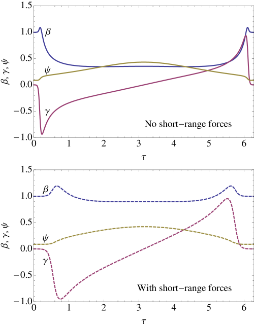
Figure 1: Shape functions $\beta$, $\gamma$, and $\psi$ for $\theta_{\rm{lb,0}}=85^{\circ}$ as a function of the rescaled time variable $\tau$, without (top panel) and with (bottom panel) short range forces. The physical parameters for the bottom panel are $M_{p}=5M_{J}$, $a_{b}=300$ AU, $a=1.5$ AU.

Due to the reduction of $e_{\mathrm{max}}$, the maximum of $\alpha(t)$ (Eq. 7) is also reduced, leading to a significant decrease in $\bar{\alpha}$ (Eq. 12). Thus, another consequence of the inclusion of short-range forces is a decrease in the parameter $N_{\mathrm{max}}$ (Eq. 24). Figure 2 (left) presents $N_{\mathrm{max}}$ as a function of the initial orbital inclination $\theta_{\rm{lb,0}}$ with and without short-range forces. We see that, in general, $N_{\mathrm{max}}$ is greatly reduced when short-range forces are included. Furthermore, because at high initial inclinations (e.g, $\theta_{\rm{lb,0}}\mathrel{\raise 1.29167pt\hbox{$>$}\mkern-14.0mu\lower 2.58334pt\hbox{$\sim$}}85$), the maximum eccentricity is determined by the short-range forces and is not sensitive to $\theta_{\rm{lb,0}}$ (e.g. Liu et al. 2015), $N_{\mathrm{max}}$ becomes nearly independent of the initial inclination. It is worth noting that $N_{\mathrm{max}}$ still scales linearly with the stellar spin rate (or inversely with the spin period), but its dependence on $M_{p}$ is no longer as simple, since $M_{p}$ now plays a role in setting the maximum eccentricity.

Likewise, the parameter $\bar{\mathcal{A}}$ is also affected (Fig. 2, right). Like $N_{\mathrm{max}}$, it still scales linearly with the stellar spin rate. However, unsurprisingly (cf. Eq. 26), it has a much stronger dependence on the initial inclination.

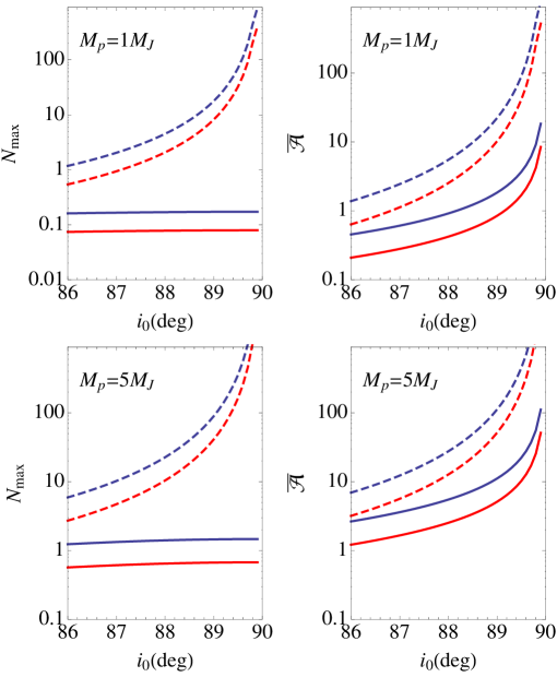
Figure 2: $N_{\rm max}$ (left panels) and $\bar{\mathcal{A}}$ (right panels) as a function of initial inclination for two planet masses (top panel: $M_{p}=1M_{J}$; bottom panel: $M_{p}=5M_{J}$) and two stellar spin periods (red: $P_{\star}=5$ days; blue: $P_{\star}=2.3$ days). Dashed: without short-range forces. Solid: with short-range forces.

For comparison, Figure 3 demonstrates how a sample phase space previously presented in SL15 (Fig. 6) changes when short-range forces are added to the system: As expected, the number of resonances is significantly reduced, and on the whole most resonances become wider. In summary, given a system with a set of initial parameters, the inclusion of short-range forces changes the shape functions that drive the spin precession dynamics, and generally decreases both $\bar{\mathcal{A}}$ and $N_{\mathrm{max}}$, reducing the degree of adiabaticity of the system.

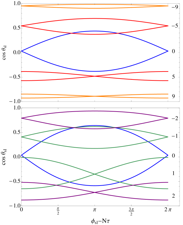
Figure 3: Separatrices in the phase space for a sample of resonances, labeled on the right-hand side with their corresponding $N$, for the shape functions presented in Fig. 1 (with $\theta_{\rm{lb,0}}=85^{\circ}$ and $\epsilon=0.1$), without (top panel) and with (bottom panel) short-range forces. Note that, for identical values of $\epsilon$ and $\theta_{\rm{lb,0}}$, inclusion of short-range forces significantly reduces the number of resonances affecting the system dynamics (i.e. the number of resonances that “fit” inside the phase space).

Finally, note that there is one more “non-ideal” effect we have neglected: the perturbation of the planet’s orbit due to the rotation-induced stellar quadrupole. This perturbation comes in two forms. First, the stellar quadrupole induces additional periastron advance in the orbit, similar to the other short-range forces. Second, the planet’s orbit experiences an extra nodal precession, governed by the equation

$$\left(\frac{d\hat{{\bf L}}}{dt}\right)_{\rm SL}=\Omega_{\rm{ps}}{S\over L}\hat{{\bf S}}\times\hat{{\bf L}},$$ (27)

where the ratio of the stellar spin angular momentum to the orbital angular momentum is

$${S\over L}\simeq 0.12\left(\!{k_{\star}\over 0.1}\!\right)\!\left(\!{M_{\star}\over M_{\odot}}\!\right)^{\!1/2}\!\left(\!{R_{\star}\over R_{\odot}}\!\right)^{2}\left(\!{M_{p}\over M_{J}}\!\right)^{\!-1}$$

$$\qquad\times\left[{a(1-e^{2})\over 0.05\,{\rm AU}}\right]^{\!-1/2}\!\left(\!{P_{\star}\over 30\,{\rm d}}\!\right)^{\!-1}.$$ (28)

We ignore these effects because, by creating feedback between stellar spin precession and orbit precession, they break the integrability of the Hamiltonian system by introducing more degrees of freedom [i.e. $e(t)$, $\Omega_{\rm{pl}}(t)$, etc. would no longer be solely determined by LK dynamics and in general would not be “known” periodic forcing functions acting on the spin evolution]. Neglecting these feedback effects is the single biggest simplifying assumption we make in our analysis. The significance of these effects increases with increasing $S/L\propto\Omega_{\star}/M_{p}$ (see Section 4.3 of ASL16 for further discussion). For low planet masses and high stellar rotation rates, this makes our subsequent analysis of the spin dynamics somewhat pedagogical. For higher planet masses and lower stellar spin rates, however, the feedback is not as important, and our conclusions should be fairly robust.

4 Non-dissipative Regime Classification

In this section we examine the differences in the spin dynamical behavior of a non-dissipative system in the non-adiabatic vs adiabatic regimes. We select two representative “shapes” of the LK orbit by considering systems with $M_{p}=5M_{J}$, $a=1.5$ AU, $a_{b}=300$ AU, and either $\theta_{\rm{lb,0}}=89^{\circ}$ or $\theta_{\rm{lb,0}}=87^{\circ}$. We then vary the stellar spin period, which scales up/down both $N_{\mathrm{max}}$ and $\bar{\mathcal{A}}$. Note that, in order to explore the entire range of possible behaviors, we consider a somewhat unphysical range of stellar spin periods, from as large as $50$ days to as small as $1$ day.

We first consider the spin dynamics in the non-adiabatic regime, with $\bar{\mathcal{A}}\mathrel{\raise 1.29167pt\hbox{$<$}\mkern-14.0mu\lower 2.58334pt\hbox{$\sim$}}1$ (section 4.1). We then consider the adiabatic regime with $\bar{\mathcal{A}}\mathrel{\raise 1.29167pt\hbox{$>$}\mkern-14.0mu\lower 2.58334pt\hbox{$\sim$}}1$ (section 4.2), which is further divided into two sub-regimes with $N_{\mathrm{max}}\mathrel{\raise 1.29167pt\hbox{$<$}\mkern-14.0mu\lower 2.58334pt\hbox{$\sim$}}1$ and $N_{\mathrm{max}}\mathrel{\raise 1.29167pt\hbox{$>$}\mkern-14.0mu\lower 2.58334pt\hbox{$\sim$}}1$ (recall that $\bar{\mathcal{A}}\mathrel{\raise 1.29167pt\hbox{$>$}\mkern-14.0mu\lower 2.58334pt\hbox{$\sim$}}N_{\mathrm{max}}$). Finally, we specialize to the dynamics of spin trajectories that start with $\cos\theta_{\rm{sl}}=1$ (i.e. zero initial spin-orbit misalignment) and discuss their behavior in each of the aforementioned regimes (section 4.3).

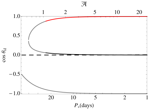
Figure 4: Locations of the fixed points of the Hamiltonian (29), for $\phi_{\rm{sl}}=0$ (solid lines) and $\phi_{\rm{sl}}=\pi$ (dashed line), for $M_{p}=5M_{J}$, $\theta_{\rm{lb,0}}=89^{\circ}$, as a function of the stellar spin period. For reference, the adiabaticity parameter $\bar{\mathcal{A}}$ is plotted on the top axis. $N_{\mathrm{max}}$ can be calculated as $N_{\mathrm{max}}\simeq\bar{\mathcal{A}}/7.63$. For more detail about the phase space structure, see Fig. 5. The colors of the lines match those of the corresponding separatrices in Fig. 5.

4.1 Non-adiabatic Regime: $\bar{\mathcal{A}}\mathrel{\raise 1.29167pt\hbox{$<$}\mkern-14.0mu\lower 2.58334pt\hbox{$\sim$}}1$

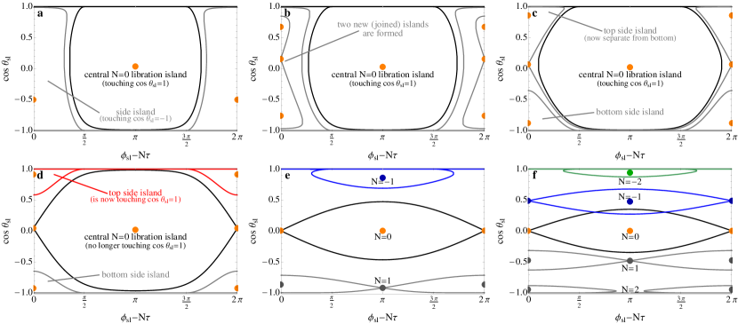
Figure 5: Sample separatrices in phase space for $M_{p}=5M_{J}$, $\theta_{\rm{lb,0}}=89^{\circ}$ and (from a to f), $P_{\star}=50$, $35$, $25$, $20$, $3$, and $1.6$ days. The separatrices shown in gray are those that have no relevance to the dynamics of the initially-aligned trajectory ($\cos\theta_{\rm{sl,0}}=1$). The colored dots mark locations of fixed points. Here $\bar{\mathcal{A}}\simeq 25.5/P_{\star}$ and $N_{\mathrm{max}}\simeq 3.34/P_{\star}$.

The form of the Hamiltonian (19) is such that the non-adiabatic regime of spin dynamics does not easily lend itself to pertubation theory and cannot be formally explored. Nevertheless, the non-adiabatic regime is very important (especially for Jupiter-mass or smaller planets). We therefore endeavor to study it based on physical arguments we consider reasonable but not necessarily rigorous.

We classify the non-adiabatic regime as having $\bar{\mathcal{A}}\mathrel{\raise 1.29167pt\hbox{$<$}\mkern-14.0mu\lower 2.58334pt\hbox{$\sim$}}1$. Since typically $\hat{\Omega}_{\rm L}\mathrel{\raise 1.29167pt\hbox{$<$}\mkern-14.0mu\lower 2.58334pt\hbox{$\sim$}}1$, this implies $N_{\mathrm{max}}\ll 1$. Thus in the non-adiabatic regime, the stellar spin vector $\hat{{\bf S}}$ changes slowly compared to both the rate of change of $\hat{{\bf L}}$ and the LK oscillation frequency. We therefore surmise that most of the relevant spin dynamics can be captured using a time-independent Hamiltonian whose coefficients are the time averages of the externally imposed shape functions ($\beta$, $\psi$, $\gamma$). In other words, most of the spin dynamics can be understood by analyzing the $N=0$ Hamiltonian (cf. Eq. 22)

$$H_{0}=N_{\mathrm{max}}\biggl{[}-\frac{1}{2}p^{2}+\frac{p}{\bar{\mathcal{B}}}-\frac{1}{2\bar{\mathcal{A}}}\sqrt{1-p^{2}}\,\cos\phi_{\rm{sl}}\biggr{]},$$ (29)

where we have replaced $\bar{\alpha}/n_{e}$ with $N_{\mathrm{max}}$, replaced $\epsilon(\beta_{0}+\gamma_{0})\equiv 2\epsilon\beta_{0}$ using the definition of $\bar{\mathcal{A}}$, and have defined $\bar{\mathcal{B}}\equiv(\epsilon\,\psi_{0})^{-1}$.

First, it is useful to examine the fixed points of the Hamiltonian $H_{0}$, and how they depend on the stellar spin period. By considering the equations of motion, it is easy to see that this Hamiltonian has two sets of fixed points: those with $\phi_{\rm{sl}}=0$ and those with $\phi_{\rm{sl}}=\pi$. Figure 4 shows how the locations of these fixed points in $\cos\theta_{\rm{sl}}$ change with stellar spin period. At very high spin periods, only two fixed points exist, one at $\phi_{\rm{sl}}=0$ and another at $\phi_{\rm{sl}}=\pi$. These fixed points are closely related to the well-known Cassini states (e.g. Fabrycky et al. 2007). At $P_{\star}\mathrel{\raise 1.29167pt\hbox{$<$}\mkern-14.0mu\lower 2.58334pt\hbox{$\sim$}}40$ days, another set of fixed points appear for $\phi_{\rm{sl}}=0$. We can now examine how each of these fixed points affects the system dynamics.

The top panels of Figure 5 present example phase spaces calculated based on the Hamiltonian (29), for which $\bar{\mathcal{A}}\mathrel{\raise 1.29167pt\hbox{$<$}\mkern-14.0mu\lower 2.58334pt\hbox{$\sim$}}1$. The curves shown in each panel are separatrices that cannot be crossed by any spin evolution trajectory. The shapes of the separatrices constrain the possible trajectories. Thus, an analysis of the separatrix shapes sheds light on the possible behaviors of the system.

At very low values of $\bar{\mathcal{A}}$ (Fig. 5, panel a), the phase space is roughly split into two islands of libration, each containing a fixed point. The separatrix of the center island touches $\cos\theta_{\rm{sl}}=1$, whereas the other touches $\cos\theta_{\rm{sl}}=-1$. A trajectory starting inside one of these separatrices will librate about the corresponding fixed point in the center of the island. Trajectories starting in the narrow region in-between the two separatrices are able to circulate.

As shown in Fig. 4, at $P_{\star}\mathrel{\raise 1.29167pt\hbox{$<$}\mkern-14.0mu\lower 2.58334pt\hbox{$\sim$}}40$ days, two more fixed points appear. Panel b of Fig. 5 shows the phase space structure shortly after the appearance of these fixed points. Two new, joined, libration islands appear. The bottom island has the previously existing Cassini-state fixed point at its center. The top island has one of the new fixed points at its center. The second new fixed point defines the separatrix between these two islands.

As $\bar{\mathcal{A}}$ gets closer to $1$ (Fig. 5, panel c), the central (centered on $\phi_{\rm{sl}}=\pi$) libration island expands, and eventually cleaves the two side islands.

As $\bar{\mathcal{A}}$ further increases, the center libration island spans an increasingly larger range of $\phi_{\rm{sl}}$, until, when $\bar{\mathcal{A}}\simeq 1$, it spans the entire $\{0,2\pi\}$ range and detaches from $\cos\theta_{\rm{sl}}=1$, forming the standard cat-eye shaped $N=0$ resonance (Fig. 5, panel d). (Note that the location of the transition is not exact: as can be seen from Fig. 5, panel c, the actual transition happens slightly after $\bar{\mathcal{A}}\simeq 1$.) The fixed point that previously defined the separatrix for the top side island now defines the separatrix for the cat-eye. At the same time, the top side island attaches to $\cos\theta_{\rm{sl}}=1$. This marks the transition from non-adiabatic to adiabatic behavior.

4.2 Adiabatic Regime: $\bar{\mathcal{A}}\mathrel{\raise 1.29167pt\hbox{$>$}\mkern-14.0mu\lower 2.58334pt\hbox{$\sim$}}1$

4.2.1 $N_{\mathrm{max}}\mathrel{\raise 1.29167pt\hbox{$<$}\mkern-14.0mu\lower 2.58334pt\hbox{$\sim$}}1$

Shortly after the non-adiabatic to adiabatic transition, $N_{\mathrm{max}}$ is still small, and therefore the spin dynamics are still essentially governed by the $N=0$ Hamiltonian. After the central $N=0$ island/resonance has detached from $\cos\theta_{\rm{sl}}=1$, the top side island merges upward and attaches to $\cos\theta_{\rm{sl}}=1$ (Fig. 5, panel d, shown in red). As $\bar{\mathcal{A}}$ and $N_{\mathrm{max}}$ continue to increase, this side island rapidly shrinks and is soon overtaken in importance by the newly forming $N=-1$ resonance. Likewise, the bottom island shrinks as well and is soon dominated by the $N=1$ resonance.

4.2.2 $N_{\mathrm{max}}\mathrel{\raise 1.29167pt\hbox{$>$}\mkern-14.0mu\lower 2.58334pt\hbox{$\sim$}}1$

As $N_{\mathrm{max}}$ approaches $1$, the spin dynamics are no longer determined solely by the $N=0$ Hamiltonian. Rather, the $N=1$ and $N=-1$ Hamiltonians must also be considered (see Eq. 22). For $0.5\mathrel{\raise 1.29167pt\hbox{$<$}\mkern-14.0mu\lower 2.58334pt\hbox{$\sim$}}N_{\mathrm{max}}\mathrel{\raise 1.29167pt\hbox{$<$}\mkern-14.0mu\lower 2.58334pt\hbox{$\sim$}}1$, each of these Hamiltonians produces a separatrix that is attached to $\cos\theta_{\rm{sl}}=1$ (for $N=-1$) and $\cos\theta_{\rm{sl}}=-1$ (for $N=1$). As $N_{\mathrm{max}}$ continues to increase, the separatrices “emerge” more fully into the phase space until eventually they detach from the top and bottom edges and form standard cat-eye shapes. Note that, due to the slight asymmetry in the Hamiltonians introduced by the $p/\bar{\mathcal{B}}$ term, the bottom resonance detaches slightly earlier than $N_{\mathrm{max}}\simeq 1$, whereas the top resonance detaches slightly later than $N_{\mathrm{max}}\simeq 1$ (Fig. 5, panel e).

After the $N=\pm 1$ resonances have emerged fully, the $N=\pm 2$ resonances begin to grow, and likewise detach and form cat-eye shapes when $N_{\mathrm{max}}\simeq 2$ (Fig. 5, panel f).

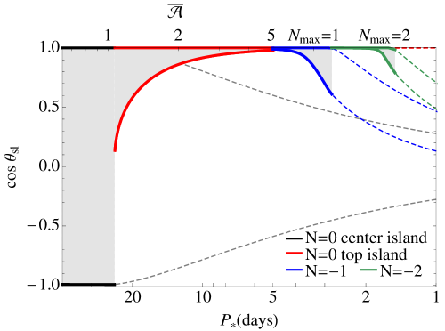
Figure 6: The range (in $\cos\theta_{\rm{sl}}$) of each of the “relevant” separatrices presented in Fig. 5 as a function of stellar spin period for $\theta_{\rm{lb,0}}=89^{\circ}$ and $M_{p}=5M_{J}$. Colors have been chosen to match those of Fig. 5. The separatrix widths are shown in bold solid lines whenever they touch $\cos\theta_{\rm{sl}}=1$ – such separatrices then determine the behavior of an initially-aligned trajectory. After detaching from $\cos\theta_{\rm{sl}}=1$, each separatrix is shown in thin dashed lines of the same color. Note that the transition from non-adiabatic behavior (controlled by the $N=0$ center island) to adiabatic behavior happens at $\bar{\mathcal{A}}\simeq 1$. In grey we show the maximum range of excursion that the initially-aligned trajectory can have. Also note that the transition from the red ($N=0$ top side island dominated) to blue ($N=-1$ dominated) is somewhat arbitrary, as there is no precise way to tell when the $N=-1$ resonance starts to dominate.

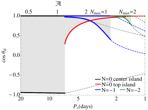
Figure 7: Same as Fig. 6, but with $\theta_{\rm{sl,0}}=87^{\circ}$.

4.3 The initially-aligned trajectory

In the standard planetary system formation scenario, giant planets are formed at a few AU’s distance from their host stars, with the orbital axis aligned with the stellar spin axis. Although in recent years several methods of generating primordial misalignment have been suggested (e.g. Bate et al. 2010; Batygin 2012; Batygin & Adams 2013; Lai 2014; Lai et al. 2011; Spalding & Batygin 2014), for the remainder of this paper we will focus on systems with $\cos\theta_{\rm sl,0}=1$, i.e. no initial spin-orbit misalignment. What determines the dynamic behavior of the stellar spin as the planet undergoes LK oscillations?

One key observation can be taken away from the six panels presented in Fig. 5: regardless of what regime the system is in, there is always a separatrix “attached” to $\cos\theta_{\rm{sl}}=1$. In the non-adiabatic regime ($\bar{\mathcal{A}}\mathrel{\raise 1.29167pt\hbox{$<$}\mkern-14.0mu\lower 2.58334pt\hbox{$\sim$}}1$) this separatrix is the $N=0$ center island. In the adiabatic regime ($\bar{\mathcal{A}}\mathrel{\raise 1.29167pt\hbox{$>$}\mkern-14.0mu\lower 2.58334pt\hbox{$\sim$}}1$), this separatrix is the $N=0$ top side island when $N_{\mathrm{max}}\mathrel{\raise 1.29167pt\hbox{$<$}\mkern-14.0mu\lower 2.58334pt\hbox{$\sim$}}0.5$ (note this number is somewhat arbitrary), and then $N=-1$ for $0.5\mathrel{\raise 1.29167pt\hbox{$<$}\mkern-14.0mu\lower 2.58334pt\hbox{$\sim$}}N_{\mathrm{max}}\mathrel{\raise 1.29167pt\hbox{$<$}\mkern-14.0mu\lower 2.58334pt\hbox{$\sim$}}1$, $N=-2$ for $1\mathrel{\raise 1.29167pt\hbox{$<$}\mkern-14.0mu\lower 2.58334pt\hbox{$\sim$}}N_{\mathrm{max}}\mathrel{\raise 1.29167pt\hbox{$<$}\mkern-14.0mu\lower 2.58334pt\hbox{$\sim$}}2$, and so on. These are the separatrices that determine the behavior of the initially aligned trajectory.

Figures 6 and 7 present a different way of visualizing this information. They show the maximum vertical extent of each of the relevant (“attached” to $\cos\theta_{\rm{sl}}=1$) separatrices as a function of the stellar spin period $P_{\star}$, for two different shape functions, with the corresponding values of $\bar{\mathcal{A}}$ and $N_{\mathrm{max}}$ given on the top axes. Since, in each case, the initially-aligned trajectory starts out on the relevant separatrix, its maximum vertical width represents the maximum range of spin-orbit misalignments that the trajectory can cover. Thus, in the non-adiabatic regime the stellar spin has the most “freedom” and is able to cover the largest range of $\cos\theta_{\rm{sl}}$. As $\bar{\mathcal{A}}$ increases, the spin axis’ range of excursion becomes progressively more and more limited, though not monotonically so.

There is a clear difference between Figures 6 ($\theta_{\rm{sl,0}}=89^{\circ}$) and 7 ($\theta_{\rm{sl,0}}=87^{\circ}$): in Fig. 6 the regions of influence of each separatrix are clearly defined and well-separated. On the other hand, in Fig. 7 it is not always clear which separatrix dominates the evolution. Furthermore, Fig. 7 features overlaps between the different separatrices, which, as we know, is a signature of chaos (see SL15). We therefore expect that for $\theta_{\rm{sl,0}}=89^{\circ}$ the spin dynamics for all stellar rotation periods should be regular and well-behaved, whereas for $\theta_{\rm{sl,0}}=87^{\circ}$ chaotic behavior may arise for certain ranges of rotation periods.

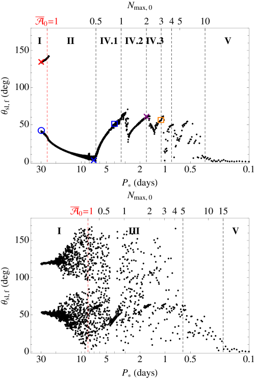
Figure 8: Final spin-orbit misalignment angle (after orbital decay and circularization due to tidal dissipation) as a function of the stellar spin period, for $M_{p}=5M_{J}$, $a_{0}=1.5$ AU, $a_{b}=300$ AU, and $\theta_{\rm{lb,0}}=89^{\circ}$ (top panel) or $\theta_{\rm{lb,0}}=87^{\circ}$ (bottom panel). The blue, red, and purple $\times$ symbols in the top panel correspond to the left, middle, and right example trajectories shown in Fig. 9, respectively. The blue $\circ$ symbol corresponds to the blue trajectory in Fig. 10. The blue and orange square symbols correspond to the left and right panels of Fig. 12, respectively. We separate identifiably distinct regions of behavior with dashed lines and number them with roman numerals.

5 Including Tidal Dissipation: Paths to Misalignment

We now include tidal dissipation in the planet and allow the semi-major axis of the planet to decay, and examine how the non-dissipative regimes discussed in the previous section map onto the final spin-orbit misalignment angle distributions. We use the standard weak friction model for tidal dissipation; see SAL14 for details.

As the planet’s semi-major axis decreases due to tidal dissipation, the stellar spin precession rate increases (Eq. 8). The LK precession rate also increases, but not as dramatically, leading to an overall gradual increase in both $\bar{\mathcal{A}}$ and $N_{\mathrm{max}}$. In addition, as the semi-major axis decays, the shape of the LK orbit changes, with the minimum eccentricity of the LK cycles slowly increasing (see Section 3.1 of ASL16); thus, the shape functions $\beta(\tau)$, $\gamma(\tau)$ and $\psi(\tau)$ that drive the stellar spin dynamics also slowly change in time. All of these changes, however, are slow enough for the system to be treated as “quasi-static”: For any given LK cycle the spin dynamics of the initially-aligned trajectory is still governed by the non-dissipative Hamiltonian, as described in the previous section. However, over the orbital decay time (involving many LK cycles), the coefficients ($N_{\mathrm{max}}$, $\bar{\mathcal{A}}$, $\bar{\mathcal{B}}$, $\beta_{M}$,$\gamma_{M}$,$\psi_{M}$) in the Hamiltonian slowly change, and the background non-dissipative phase space slowly evolves through a sequence similar to that depicted in Figs. 5, 6 and 7.

There are two consequences of this slow evolution of the Hamiltonian coefficients. First, since at any given time the system is still governed by a Hamiltonian, a (non-chaotic) trajectory still cannot cross a separatrix (unless it has no choice – more on this later). The implication is that if a trajectory starts out inside a certain separatrix, its behavior will continue to be governed by that (slowly evolving) separatrix. Second, because the system evolves so gradually (or adiabatically - not to be confused with the adiabatic regime!), an adiabatic invariant emerges: the area enclosed by a trajectory in the $\cos\theta_{\rm{sl}}-(\phi_{\rm{sl}}-N\tau)$ space is an approximately conserved quantity. Together, these two ideas (avoidance of separatrix crossings, and conservation of area) are all that is necessary to understand the dissipative system. Thus, in principle, knowing what separatrix governs the behavior of the initially-aligned system at $t=0$, plus the knowledge of how that separatrix changes under the influence of tidal evolution, should be enough to determine the fate of the trajectory.

The above considerations indicate that the governing separatrix at $t=0$ determines the fate of an initially aligned system. The initial separatrix is specified by the parameters (see Section 4.3)

$$\bar{\mathcal{A}}_{0}\equiv\bar{\mathcal{A}}(t=0),\quad N_{\rm max,0}\equiv N_{\mathrm{max}}(t=0).$$ (30)

In the presence of tidal dissipation, we expect that all possible outcomes of the system may be classified using these two parameters.

5.1 Varying the stellar spin period

We begin by repeating the experiment of Section 4, including the influence of tides and numerically integrating the system until the planet orbit decays and circularizes. We select two initial ($t=0$) “shapes” for the LK orbit by setting $M_{p}=5M_{J}$, $a_{0}=1.5$ AU (the initial semi-major axis), $a_{b}=300$ AU, and either $\theta_{\rm{lb,0}}=89^{\circ}$ or $\theta_{\rm{lb,0}}=87^{\circ}$. For $t>0$, the “shape” of the orbit slowly evolves (as the semi-major axis shrinks). As in Section 4, we vary the stellar spin period (which remains constant throughout the tidal evolution). We set $\theta_{\rm sl,0}=0$ and plot $\theta_{\rm sl,f}$, the final spin-orbit misalignment angle, as a function of the stellar spin period in Figure 8. As before, we cover a somewhat unphysical range of stellar spin periods in order to capture all possible behaviors and outcomes.

Five distinct categories of outcomes in Fig. 8 can be identified:

(I) The distinct bimodal distribution at very high spin periods ($P_{\star}\mathrel{\raise 1.29167pt\hbox{$>$}\mkern-14.0mu\lower 2.58334pt\hbox{$\sim$}}23$ days and $P_{\star}\mathrel{\raise 1.29167pt\hbox{$>$}\mkern-14.0mu\lower 2.58334pt\hbox{$\sim$}}9$ days in Fig. 8 upper and lower panels, respectively);

(II) The unimodal, monotonically decreasing distribution at high to intermediate spin periods ($7\mathrel{\raise 1.29167pt\hbox{$<$}\mkern-14.0mu\lower 2.58334pt\hbox{$\sim$}}P_{\star}\mathrel{\raise 1.29167pt\hbox{$<$}\mkern-14.0mu\lower 2.58334pt\hbox{$\sim$}}20$ days in Fig. 8, upper panel);

(III) The region of wide-spread chaos ($0.5\mathrel{\raise 1.29167pt\hbox{$<$}\mkern-14.0mu\lower 2.58334pt\hbox{$\sim$}}P_{\star}\mathrel{\raise 1.29167pt\hbox{$<$}\mkern-14.0mu\lower 2.58334pt\hbox{$\sim$}}9$ days in Fig. 8 lower panel);

(IV) The diagonally striated pattern of spin-orbit misalignments at low and very low spin periods ($0.5\mathrel{\raise 1.29167pt\hbox{$<$}\mkern-14.0mu\lower 2.58334pt\hbox{$\sim$}}P_{\star}\mathrel{\raise 1.29167pt\hbox{$<$}\mkern-14.0mu\lower 2.58334pt\hbox{$\sim$}}7$ days in Fig. 8 upper panel); we term this behavior “adiabatic advection” and discuss it extensively below;

(V) The region of very exceptionally small final misalignments at very low spin periods ($P_{\star}\mathrel{\raise 1.29167pt\hbox{$<$}\mkern-14.0mu\lower 2.58334pt\hbox{$\sim$}}0.4$ days and $P_{\star}\mathrel{\raise 1.29167pt\hbox{$<$}\mkern-14.0mu\lower 2.58334pt\hbox{$\sim$}}0.3$ days in the upper and lower panels of Fig. 8, respectively).

Figure 9 illustrates the time evolution for the behaviors (I), (II) and (IV). We discuss each category of outcomes individually in the following subsections.

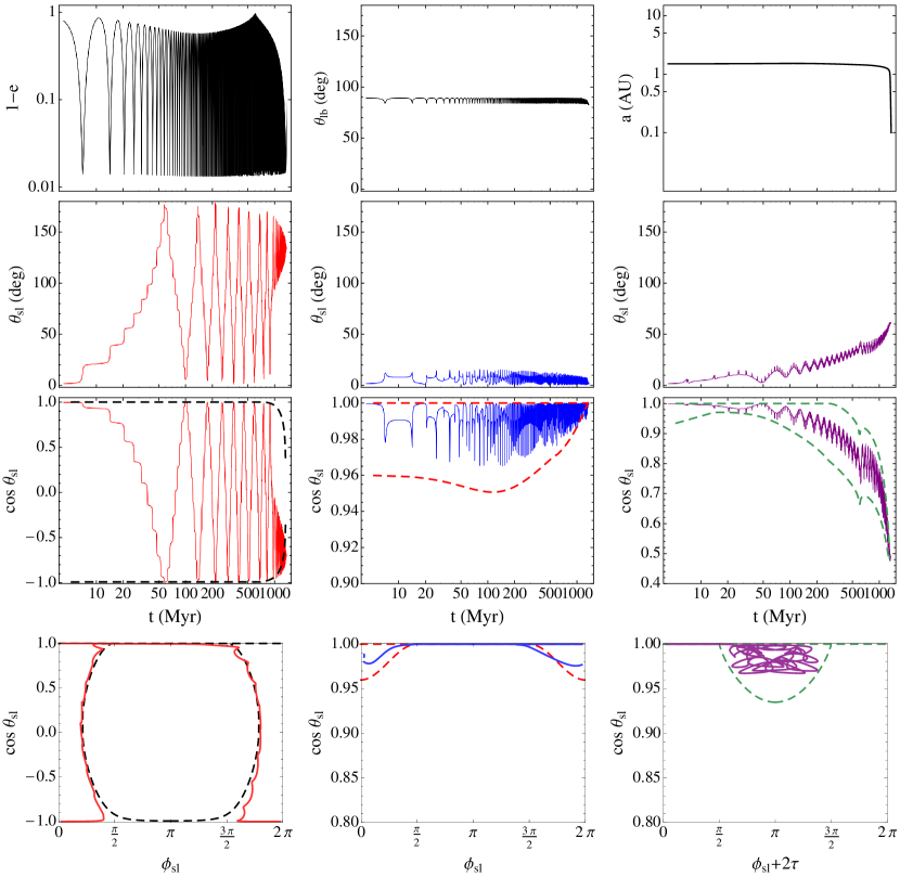
Figure 9: Sample evolution trajectories, including tidal dissipation, for $\theta_{\rm{lb,0}}=89^{\circ}$, $M_{p}=5M_{J}$ and three different values of the stellar spin period. Left panels: $P_{\star}=30$ days; middle panels: $P_{\star}=7.07$ days; right panels: $P_{\star}=1.67$ days. Top row: evolution of the orbital elements (the planet’s eccentricity, orbital inclination relative to the outer binary, and the semi-major axis). The orbital elements’ evolution is independent of the stellar spin period and is therefore the same for all three cases. Second row: evolution of the spin-orbit misalignment angle $\theta_{\rm{sl}}$. Third row: evolution of $\cos\theta_{\rm{sl}}$ (solid lines) as well as the relevant background separatrix (dashed lines; see next). Bottom row: the initial background phase space separatrices (dashed lines; see Fig 5) as well as the first full cycle of evolution of the trajectory (solid lines), showing that the relevant background separatrices, from left to right, are the $N=0$ center island (shown in black-dashed line), the $N=0$ top island (shown in red-dashed line), and the $N=-2$ resonance (shown in green-dashed line).

5.2 Non-adiabatic behavior: bimodality (I)

We first address the clean bimodal spin-orbit misalignment distribution found at high stellar spin periods in Fig. 8 (upper panel). In order to understand its origin, we need to know which separatrix governs the behavior of the $\theta_{\rm sl,0}=0$ trajectory at $t=0$. Two simple clues point to the answer: First, the left panels of Fig. 9 show an example of the time evolution in the bimodal regime, as well as the $t=0$ phase space for that evolution. We see that the separatrix governing the behavior of the trajectory at $t=0$ is the $N=0$ central island. Second, in Fig. 8 the bimodal region ends very close to $\bar{\mathcal{A}}_{0}\simeq 1$, i.e. at the stellar spin period for which at $t=0$ we have $\bar{\mathcal{A}}\simeq 1$. From Section 4, we know that $\bar{\mathcal{A}}\simeq 1$ corresponds to the transition between the non-adiabatic and adiabatic behavior, and that at $\bar{\mathcal{A}}\simeq 1$ the governing separatrix for the initially aligned system switches from being the $N=0$ center island to the $N=0$ top island (see Fig. 5 and Fig. 6). Thus, the bimodality found at high stellar spin periods in Fig. 8 corresponds to the initially non-adiabatic regime.

To understand why the outcome is bimodal, we now need to know two things: how the $N=0$ center separatrix changes in time (due to tidal dissipation), and how the trajectory interacts with it.

The $N=0$ center separatrix evolves in time (Fig. 9, left, the third panel from the top) in a way exactly analogous to the sequence shown in Figs. 5 and 6: Initially the separatrix is attached to $\cos\theta_{\rm{sl}}=1$. As tidal dissipation acts to reduce the semi-major axis and increase $\bar{\mathcal{A}}$ and $N_{\mathrm{max}}$, the separatrix detaches from $\cos\theta_{\rm{sl}}=1$ and slowly shrinks. On the other hand, the actual trajectory cannot shrink, due to the aforementioned adiabatic invariance of the area it encloses in the phase space. Its initial area is set by the area of the separatrix at $t=0$. At intermediate times the separatrix actually expands (analogously to the transition between panels a and b of Fig. 5) and the trajectory remains inside the separatrix. After the separatrix detaches and begins to shrink again, there comes a point when the area of the separatrix is equal to the area of the trajectory. At that point, the trajectory has no choice but to cross the separatrix.

Figure 10 illustrates this idea. At time of crossing, the trajectory can cross either the top or the bottom part of the separatrix, depending on its phase. Two trajectories that start very close together can, over time, accumulate enough difference in phase that one ends up exiting through the top, and the other through the bottom. This is the origin of the bimodality seen in Fig. 8.

This “bifurcation” phenomenon is analogous to the case of a pendulum whose length is slowly decreased with time. The shorter the pendulum gets, the larger its amplitude of oscillation becomes, until at some point it must transition to circulating rather than oscillating. At that point, the pendulum will “choose” to circulate either clockwise or counterclockwise – corresponding to a positive or negative conjugate momentum – depending on its phase at the time of transition.

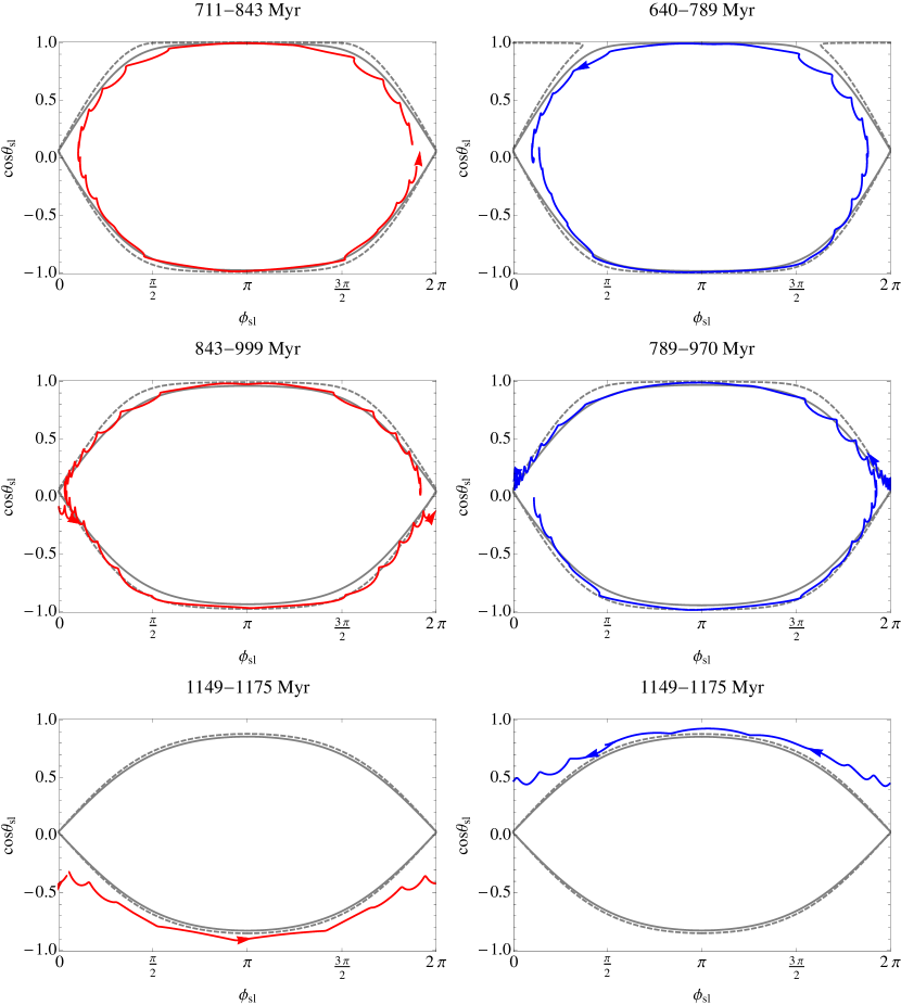
Figure 10: Demonstration of the process that gives rise to the bimodality found in the non-adiabatic regime of Fig. 8 (top panel). In each panel, the dashed (solid) grey line shows the $N=0$ separatrix at the beginning (end) of the time interval indicated at the top of the panel, while the colored line shows the actual time evolution of $\cos\theta_{\rm{sl}}$ during that time interval. The red line (left panels) has $P_{\star}=30$ days and is the trajectory shown in the left panels of Fig. 9 and marked with a red X in Fig. 8. The blue line (right panels) has $P_{\star}=29.87$ days and is marked with a blue O in Fig. 8. Top panels: both trajectories are contained within the $N=0$ separatrix and their areas are smaller than the separatrix area. Middle panels: the $N=0$ separatrix has shrunk such that its area now matches the areas of the trajectories, thus the trajectories have no choice but to exit the resonance. The red (blue) trajectory’s location at time of exit is such that it exits below (above) the separatix. Bottom panels: both trajectories are now caught in their respective part of phase space.

Finally, we note that while the bimodality is very clear and distinct in the upper panel of Fig. 8, it becomes increasingly disordered at lower periods in the lower panel of Fig. 8. This is the onset of widespread chaos that arises from resonance overlaps, as discussed in Section 4.3 (see SL15).

5.3 Stationary adiabatic behavior (II)

For $\bar{\mathcal{A}}_{0}\mathrel{\raise 1.29167pt\hbox{$>$}\mkern-14.0mu\lower 2.58334pt\hbox{$\sim$}}1$ and $N_{\rm max,0}\mathrel{\raise 1.29167pt\hbox{$<$}\mkern-14.0mu\lower 2.58334pt\hbox{$\sim$}}0.5$, Fig. 8 (top panel) shows a smooth unimodal distribution of final spin-orbit misalignments, with $\theta_{\rm sl,f}$ decreasing with decreasing $P_{\star}$. In Section 5.2, we have already determined that the behavior in this regime must be governed by the $N=0$ top side island. The middle bottom panel of Fig. 9 shows that this is indeed the case. In order to understand the distribution of the final misalignments, we again need to ask how the $N=0$ top separatrix evolves with time, and how the trajectory interacts with it.

Based on Fig. 6, we know that an increase in $\bar{\mathcal{A}}$ or $N_{\mathrm{max}}$ leads to a rapid decrease in the width of the $N=0$ top island. On the other hand, again, the actual trajectory area is constant and set by the initial area of the top island. Thus, as soon as any significant semi-major axis decay occurs, the trajectory area will exceed the area of the top island, and the actual trajectory should circulate on the outside of the island. For a circulating trajectory, the new conserved area becomes the area between the trajectory and the $\cos\theta_{\rm{sl}}=0$ axis. Thus, as more semi-major axis decay occurs, the trajectory cannot move up/down, it can only straighten out, eventually settling on a constant $\cos\theta_{\rm sl,f}$ equal approximately to its mean $\cos\theta_{\rm{sl}}$ value at the time of decoupling from the top island.

Thus, if the top island is initially extended, the final $\theta_{\rm sl,f}$ should be (relatively) large. As the stellar spin period decreases, the top island decreases in size; therefore, $\theta_{\rm sl,f}$ gets closer and closer to $0$.

A caveat to the above discussion is the following: Further into the adiabatic regime, the assumption that only the $N=0$ Hamiltonian determines the spin dynamics becomes increasingly erroneous, since the stellar spin vector now precesses at at rate comparable to the precession of $\hat{{\bf L}}$ and thus sees more than just the time average of the forcing functions. Thus, although the above discussion is suggestive and sound, the actual behavior of the trajectory can be more random and need not obey these rules. This is why, for example, the trajectory depicted in the middle column of Fig. 9 actually remains level with, or inside, the top island for most of its evolution.

We term this regime of behavior “stationary adiabatic” because the trajectory essentially cannot move away from its initial location. This is to be contrasted with type (IV) behavior discussed below.

Note that type (II) behavior need not always be present: for example, there is no such apparent behavior in the bottom panel of Fig. 8. This is because, in many cases, it can be replaced by wide-spread chaos, as discussed below.

5.4 Widespread Chaos (III)

For intermediate values of the stellar spin period, in the lower panel of Fig. 8 we can identify a region of widespread or near widespread in the final spin-orbit misalignments, as a result of chaotic spin evolution. This type of behavior was extensively studied in SL15 and we give only a short discussion here.

As discussed in SL15, chaotic behavior often arises from resonance overlaps. In Section 4.3, based on Fig. 7 which shows the existence of resonance overlaps for certain spin periods, we suggested that misalignment distributions computed using this particular set of “shape” functions should exhibit chaotic regions. This is indeed the case. In fact, there is good agreement between Fig. 7 and the lower panel of Fig. 8: For example, for $3.5\mathrel{\raise 1.29167pt\hbox{$<$}\mkern-14.0mu\lower 2.58334pt\hbox{$\sim$}}P_{\star}\mathrel{\raise 1.29167pt\hbox{$<$}\mkern-14.0mu\lower 2.58334pt\hbox{$\sim$}}5$ days the behavior of the trajectory should be governed by the $N=-1$ resonance and this resonance does not overlap with the $N=0$ island. Thus, there is no chaos in this period range.

In general, we expect the appearance of chaos to be correlated with the widths of the resonances. Since the widths of the resonances generally decrease with increasing $\bar{\mathcal{A}}_{0}$ (see SL15), we expect the chaotic bands to be confined to lower values of $\bar{\mathcal{A}}_{0}$.

We note, however, that we cannot readily explain the existence of widespread chaos in the $P_{\star}>5$ days region of Fig. 8. This is because our resonance overlap analysis (SL15) assumes that the system is already quite adiabatic, so that any non-adiabatic effects can be treated perturbatively. For $P_{\star}>5$ days this is not the case, since $\bar{\mathcal{A}}_{0}$ is close to or less than $1$.

5.5 Adiabatic Advection (IV)

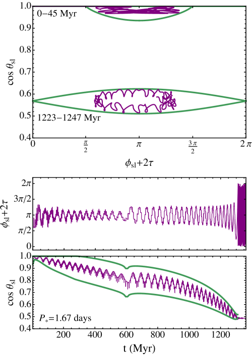
Figure 11: Demonstration of the process of adiabatic advection by an $N=-2$ resonance. In both panels, the purple lines show the actual time evolution of the spin trajectory, corresponding to the right panels of Fig. 9, and is marked with a purple X in Fig. 8. Top panel: the median shape of the $N=-2$ resonance and the time evolution of $\cos\theta_{\rm{sl}}$ is shown at two different time intervals. In both intervals, the actual trajectory is contained inside the resonance. Bottom panel: the full evolution of $\phi_{\rm sl}+2\tau$ (top sub-panel) and $\cos\theta_{\rm{sl}}$ (bottom sub-panel, purple) as well as the maximum width of the $N=-2$ resonance vs time (bottom sub-panel, green), confirming that the trajectory advects with the resonance until the resonance shrinks significantly and the trajectory has no choice but to exit.

The concept of adiabatic advection was first considered by SL15 in a schematic manner. Here we demonstrate that adiabatic advection indeed applies in the realistic situation of “LK oscillation + tidal decay” considered in this paper. Adiabatic advection is a novel way of generating spin-orbit misalignment.

The idea of adiabatic advection is simple: If at $t=0$ the behavior of the $\cos\theta_{\rm sl,0}=1$ trajectory is governed by a resonance with a specific $N$ ($=-1,-2,\cdots$), then as tidal dissipation reduces the semi-major axis of the orbit, the trajectory can be advected by the governing resonance to non-zero misalignments. Figure 11 shows an example of this behavior: in the top panel, at $t=0$ we see that the trajectory is trapped inside the $N=-2$ resonance, which is still “attached” to $\cos\theta_{\rm{sl}}=1$. Over a Gyr later, the resonance has detached and moved down significantly, and the trajectory has likewise moved down and remains inside the resonance, producing a significant spin-orbit misalignment.

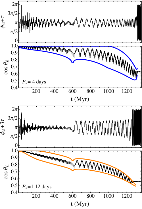
Figure 12: Demonstration of the process of adiabatic advection by the $N=-1$ (top) and the $N=-3$ (bottom) resonance. The top (bottom) time evolution is marked in Fig. 8 with a blue (orange) square symbol. As in Fig. 11 the two sample trajectories remain trapped in their respective resonances (top: $N=-1$, shown in blue; bottom: $N=-3$, shown in orange) and are advected with them.

Figure 13: Final spin-orbit misalignment angle as a function of initial orbital inclination $\theta_{\rm{lb,0}}$, for two different planet masses and two stellar spin periods. The $M_{p}=1M_{J}$ panels (left) exhibit non-adiabatic bimodal (I) and stationary adiabatic (II) behaviors, with the transition from one to the other occuring, as expected, at $\bar{\mathcal{A}}_{0}\simeq 1$. The $M_{p}=5M_{J}$ panels (right) exhibit chaos (III) and adiabatic advection (IV) by the $N=-2$ (top) and $N=-1$ (bottom) resonances. Because $N_{\rm max,0}$ is rather insensitive to the initial inclination (see Fig. 2), the final misalignment angle after advection is nearly independent of $\theta_{\rm{lb,0}}$. The higher mass planets also show a full adiabatic region (V).

As another means of looking at the situation, we note that at the center of the $N$-th resonance we have, by definition, $\phi_{\rm{sl}}-N\tau=0$. Thus, a trajectory trapped inside the resonance librates about this point; that is, $\phi_{\rm{sl}}-N\tau$ of such a trajectory should exhibit moderate variation about $0$. In the lower panel of Fig. 11, we show that this is indeed the case: $\phi_{\rm{sl}}+2\tau$ oscillates about $0$, indicating that the trajectory is trapped inside the $N=-2$ resonance. Likewise, the oscillations of $\cos\theta_{\rm{sl}}$ never exceed the maximum width of the $N=-2$ resonance, demonstrating that the trajectory is always contained inside.

Similarly, Figure 12 shows sample advections by the $N=-1$ (top) and $N=-3$ (bottom) resonances. By locating these examples on the $\theta_{\rm sl,f}$ vs $P_{\star}$ plot (Fig. 8, upper panel), we conclude that each of the diagonally striated lines in the top panel of Fig. 8, located at $0.5\mathrel{\raise 1.29167pt\hbox{$<$}\mkern-14.0mu\lower 2.58334pt\hbox{$\sim$}}N_{\rm max,0}\mathrel{\raise 1.29167pt\hbox{$<$}\mkern-14.0mu\lower 2.58334pt\hbox{$\sim$}}1$, $1\mathrel{\raise 1.29167pt\hbox{$<$}\mkern-14.0mu\lower 2.58334pt\hbox{$\sim$}}N_{\rm max,0}\mathrel{\raise 1.29167pt\hbox{$<$}\mkern-14.0mu\lower 2.58334pt\hbox{$\sim$}}2$, etc., corresponds to advection by a resonance of a different $N$.

5.6 Fully Adiabatic Evolution (V)

For very low (extremely fast) spin periods, the systems presented in both panels of Fig. 8 are fully adiabatic. (We note that in the particular case of Fig. 8 the spin periods in this regime are unphysically short; however, the same behavior can be achieved at more reasonable spin periods by changing the system orbital parameters or planet mass.) In this regime, the stellar spin vector has no trouble following the planet angular momentum vector as it undergoes LK oscillations, and no spin-orbit misalignment is generated. We note that, while we understand what happens in this regime, it is difficult to pinpoint its onset, i.e. the value of $P_{\star}$ or perhaps $N_{\mathrm{max}}$ for which it starts.

6 Predictive Power of the Theory

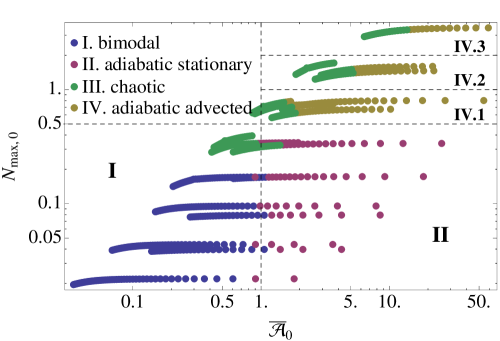
Figure 14: Compilation of the outcomes of a suite of time evolutions with variable initial conditions and parameters, plotted in the $N_{\rm max,0}$ vs $\bar{\mathcal{A}}_{0}$ space. Each outcome is classified into the categories discussed in Section 5. With dashed lines and roman numerals we denote which type of outcome we expect in that region of parameter space. The variable initial conditions/parameters include combinations of various planet masses, stellar spin periods, binary separations, and initial orbital inclinations. Despite varying all of these parameters, we see that the outcomes still agree with our expectations based on Section 5: The non-adiabatic bimodal (I) and adiabatic stationary (II) behaviors occur at low $N_{\rm max,0}$, and are separated by $\bar{\mathcal{A}}_{0}\simeq 1$. At higher $N_{\rm max,0}$, adiabatic advection (IV) and chaotic behavior (III) become possible, with the chaotic behavior being restricted to lower values of $\bar{\mathcal{A}}_{0}$ (for which, generally speaking, all the resonances are wider and more likely to overlap).

In the previous two sections, we have focused on numerical experiments that change the spin dynamics in the simplest way possible: by varying the stellar spin period, while keeping all other system parameters fixed. We would now like to check whether the understanding of the different outcomes for $\theta_{\rm sl,f}$ we have developed in the previous sections holds up when we vary some other parameters of the system. Thus, in Fig. 13 we present the distributions of final spin-orbit misalignment angles as a function of the initial orbital inclination $\theta_{\rm{lb,0}}$, for two values of the stellar spin period and two planet masses.

We find that, indeed, our classification of the misalignment outcomes based on $\bar{\mathcal{A}}_{0}$ and $N_{\rm max,0}$ holds up well. For Jupiter-mass planets, the outcomes are either bimodal (type I) or stationary adiabatic (type II), with the transition between the two regimes occuring at $\bar{\mathcal{A}}_{0}\simeq 1$, as expected. For the heavier, $5M_{J}$ planets, a chaotic band (III) appears at lower inclinations, likely due to resonance overlaps. Aside from that, however, in the non-chaotic regions we find that $\theta_{\rm sl,f}$ is nearly constant, consistent with the fact that $N_{\rm max,0}$ is moderately large and nearly independent of $\theta_{\rm{lb,0}}$ (as expected based on Fig. 2). Based on the values of $N_{\rm max,0}$, we infer that the top right panel of Fig. 13 shows an extended region of adiabatic advection by the $N=-2$ resonance (type IV.2 behavior), whereas the bottom right panel of Fig. 13 shows a region of advection by the $N=-1$ resonance (type IV.1 behavior).

Finally, taking one step further, we carry out a suite of calculations for the “LK oscillation + tidal decay” time evolutions, with various initial conditions and parameters (different planet masses, stellar spin periods, binary separations, and initial orbital inclinations). We categorize each time evolution according to its misalignment outcome: bimodal (I), stationary adiabatic (II), chaotic (III) or adiabatically advected (IV), and plot these outcomes in the $N_{\rm max,0}$ vs $\bar{\mathcal{A}}_{0}$ space (Fig. 14). From this figure, it is clear that our understanding of the different outcomes is sound: at $\bar{\mathcal{A}}_{0}\mathrel{\raise 1.29167pt\hbox{$<$}\mkern-14.0mu\lower 2.58334pt\hbox{$\sim$}}1$, bimodality dominates; at $\bar{\mathcal{A}}_{0}\mathrel{\raise 1.29167pt\hbox{$>$}\mkern-14.0mu\lower 2.58334pt\hbox{$\sim$}}1$ but $N_{\rm max,0}\mathrel{\raise 1.29167pt\hbox{$<$}\mkern-14.0mu\lower 2.58334pt\hbox{$\sim$}}0.5$ stationary adiabatic behavior is prevalent; for $\bar{\mathcal{A}}_{0}\mathrel{\raise 1.29167pt\hbox{$>$}\mkern-14.0mu\lower 2.58334pt\hbox{$\sim$}}1$ and $N_{\rm max,0}\mathrel{\raise 1.29167pt\hbox{$>$}\mkern-14.0mu\lower 2.58334pt\hbox{$\sim$}}0.5$, adiabatic advection is dominant, except where the evolution is chaotic, with the chaotic evolution restricted to lower values of $\bar{\mathcal{A}}_{0}$.

We conclude that in general, the two parameters, $\bar{\mathcal{A}}_{0}$ and $N_{\rm max,0}$, completely determine the evolutionary behavior of the spin-orbit misalignment and whether the final misalignment angle of a given system can be high. For $\bar{\mathcal{A}}_{0}\mathrel{\raise 1.29167pt\hbox{$<$}\mkern-14.0mu\lower 2.58334pt\hbox{$\sim$}}1$ (regime I), the final misalignment distribution is bimodal, and thus a system is equally likely to have low misalignment as high misalignment. For $\bar{\mathcal{A}}_{0}\mathrel{\raise 1.29167pt\hbox{$>$}\mkern-14.0mu\lower 2.58334pt\hbox{$\sim$}}1$ but $N_{\rm max,0}\mathrel{\raise 1.29167pt\hbox{$<$}\mkern-14.0mu\lower 2.58334pt\hbox{$\sim$}}0.5$ (regime II) the system is incapable of achieving a significantly misaligned state. For $\bar{\mathcal{A}}_{0}\mathrel{\raise 1.29167pt\hbox{$>$}\mkern-14.0mu\lower 2.58334pt\hbox{$\sim$}}1$ and $N_{\rm max,0}\mathrel{\raise 1.29167pt\hbox{$>$}\mkern-14.0mu\lower 2.58334pt\hbox{$\sim$}}0.5$ a calculation of resonance widths must be carried out to determine whether the system is chaotic (III) or advecting (IV), but in general it can be expected that if $\bar{\mathcal{A}}_{0}$ is relatively high then the system is not chaotic, and will attain non-zero, but strictly prograde and fairly modest, misalignment.

7 Discussion

7.1 Complications due to Spin Feedback on Orbit

As explained in Section 3, a major assumption in the analysis laid out in this paper, as well as in SL15, is the omission of the extra precession the planet’s orbit experiences due to perturbation from the stellar quadrupole. This omission enables us to considerably simplify the spin dynamics problem by reducing it to a 1D Hamiltonian system. Stellar feedback on planet’s orbit becomes important if the host star has nearly as much, or more, angular momentum as the planet’s orbit (see Eq. 28). Thus, one may question whether our analysis is truly applicable to Jupiter-mass (as opposed to heavier) planets and rapidly rotating stars. However, in ASL16 we have run a comprehensive suite of numerical simulations including stellar feedback on the orbit and all other important effects. We found that, while under certain conditions the bimodal and stationary adiabatic behaviors expected to dominate for Jupiter-mass planets can be disrupted, on the whole, bimodality remains nearly ubiquitous. We conclude that our classification of the different misalignment evolution modes and outcomes is generally valid.

7.2 Stellar Spindown

In this work, we have assumed that the stellar spin remains constant throughout the proto-HJ’s tidal decay and circularization. In reality, solar-type stars experience significant spindown due to magnetic winds. This spindown acts to temporarily reduce the strength of the coupling between the stellar spin and the planet orbit, decreasing both $N_{\mathrm{max}}$ and $\bar{\mathcal{A}}$. However, it is still the initial values of these parameters ($N_{\rm max,0}$ and $\bar{\mathcal{A}}_{0}$) that set the qualitative behavior of the system. Some differences in the final value of the spin-orbit misalignment angle $\theta_{\rm sl,f}$ due to stellar spindown could be expected, but the regime classification and predictive power should remain unchanged.

7.3 Primordial Misalignment

In this paper we have focused on stellar spin dynamics in systems that have no initial spin-orbit misalignment. However, since several ways of generating primordial misalignment have been proposed (see references in Section 1), the dynamics of initially misaligned systems are of potential interest.

Although a thorough exploration of the dynamics of initially misaligned systems is beyond the scope of this work, we believe the ideas developed in this paper, particularly the importance of the parameters $\bar{\mathcal{A}}_{0}$ and $N_{\rm max,0}$, are still applicable to initially misaligned systems. The fate of such systems should still be determined by the initial phase space of the system and where in that phase space the system is initialized. For example, for trajectories starting anywhere inside the $N=0$ center island (see Fig. 5), the final outcome should be bimodal, just as for initially aligned systems; the only difference is that, for an initially misaligned system, the peaks of the bimodal distribution of the final misalignment angle would lie closer to $90^{\circ}$ due to the smaller initial area of the trajectory. In Fig. $26$ of ASL16 we have demonstrated that this is the case.

Thus, the frameworks developed in this paper for the special case of initially aligned systems can be easily generalized to systems with arbitrary initial misalignments and phases.

8 Summary

We have developed an analytical theory to explore and classify the various regimes of stellar spin dynamics driven by planets undergoing Lidov-Kozai migration. In our previous work (Storch & Lai 2015) we analyzed only the idealized non-dissipative Lidov-Kozai system in the adiabatic regime (when the spin precession frequency is higher than the LK oscillation frequency) and succeeded in explaining the origin of chaotic behavior of stellar spin. In this paper we have significantly expanded our analysis to include the effects of various short-range forces (e.g., apsidal precession of the planet’s orbit due to General Relativity and tidal bulge) and considered all possible spin dynamical regimes. Most importantly, we have included tidal dissipation in the planet, which allows us to examine the long-term evolution of the spin-orbit misalignment angle as the planet migrates in semi-major axis and becomes a hot Jupiter. The work presented here provides a solid theoretical understanding for the various pathways toward spin-orbit misalignments as revealed in our extensive numerical simulations (Storch, Anderson & Lai 2014; Anderson, Storch & Lai 2016).

We find that, in general, the behavior of a “stellar spin + planet + binary” system with a given set of initial conditions, planet mass, and stellar spin rate is governed primarily by two parameters (Section 4): $N_{\mathrm{max}}$ (Eq. 24), which compares $\bar{\alpha}$, the average maximum precession frequency of the stellar spin, with the LK eccentricity oscillation frequency, and $\bar{\mathcal{A}}$ (Eq. 26), which compares $\bar{\alpha}$ with the averaged rate of change of the planet’s orbital angular momentum vector $\hat{{\bf L}}$. For $\bar{\mathcal{A}}\mathrel{\raise 1.29167pt\hbox{$<$}\mkern-14.0mu\lower 2.58334pt\hbox{$\sim$}}1$ (which implies $N_{\mathrm{max}}\ll 1$), the spin dynamics is in the non-adiabatic regime. The adiabatic regime ($\bar{\mathcal{A}}\mathrel{\raise 1.29167pt\hbox{$>$}\mkern-14.0mu\lower 2.58334pt\hbox{$\sim$}}1$) is divided into two sub-regimes with $N_{\mathrm{max}}\mathrel{\raise 1.29167pt\hbox{$<$}\mkern-14.0mu\lower 2.58334pt\hbox{$\sim$}}1$ and $N_{\mathrm{max}}\mathrel{\raise 1.29167pt\hbox{$>$}\mkern-14.0mu\lower 2.58334pt\hbox{$\sim$}}1$ (recall that $\bar{\mathcal{A}}\mathrel{\raise 1.29167pt\hbox{$>$}\mkern-14.0mu\lower 2.58334pt\hbox{$\sim$}}N_{\mathrm{max}}$). Each of these regimes and sub-regimes has a different phase-space resonance structure (see Figs. 5-7), which governs the evolution of the system.

In the presence of tidal dissipation (Section 5), $N_{\mathrm{max}}$ and $\bar{\mathcal{A}}$ vary slowly with time, but the fate of the system is entirely determined by the values of these parameters at $t=0$ (i.e. during the first LK cycle). In general, five distinct spin-orbit evolutionary behaviors and outcomes are possible (see Section 5.1), and Fig. 8, 13 and 14 summarize these various types of outcomes. We find that when $\bar{\mathcal{A}}_{0}\mathrel{\raise 1.29167pt\hbox{$<$}\mkern-14.0mu\lower 2.58334pt\hbox{$\sim$}}1$ (implying $N_{\rm max,0}\ll 1$), the final spin-orbit misalignment distribution is bimodal (type I), and thus the system is equally likely to settle into a retrograde or prograde orbit. When $\bar{\mathcal{A}}_{0}\mathrel{\raise 1.29167pt\hbox{$>$}\mkern-14.0mu\lower 2.58334pt\hbox{$\sim$}}1$ and $N_{\rm max,0}\mathrel{\raise 1.29167pt\hbox{$<$}\mkern-14.0mu\lower 2.58334pt\hbox{$\sim$}}0.5$, the system experiences “stationary adiabatic” behavior (type II) and cannot achieve very high (retrograde) misalignments. When When $\bar{\mathcal{A}}_{0}\mathrel{\raise 1.29167pt\hbox{$>$}\mkern-14.0mu\lower 2.58334pt\hbox{$\sim$}}1$ and $N_{\rm max,0}\mathrel{\raise 1.29167pt\hbox{$>$}\mkern-14.0mu\lower 2.58334pt\hbox{$\sim$}}0.5$, the system is either chaotic (type III) or experiences “adiabatic advection” (type IV), wherein it can slowly accumulate a modest amount of spin-orbit misalignment (never more than $90^{\circ}$). The chaotic regime is typically restricted to lower values of $\bar{\mathcal{A}}_{0}$. At very high values of both $\bar{\mathcal{A}}_{0}$ and $N_{\mathrm{max}}$ the system is fully adiabatic (type V) and cannot accumulate any misalignment.

Overall, the theoretical work presented in this paper and in Storch & Lai (2015) complements our own numerical Monte-Carlo studies of hot Jupiter formation via Lidov-Kozai migration in stellar binaries (Storch et al. 2014; Anderson et al. 2016) and those by others (e.g. Fabrycky & Tremaine 2007; Correia et al. 2011; Petrovich 2015). Our theory provides a framework to understand some of the intriguing numerical results on the final spin-orbit misalignment distributions. For example, we have shown that the bimodal distribution, seen in some of the simulations of Fabrycky & Tremaine (2007), Correira et al. (2011) and Storch et al. (2014), arises naturally from a “bifurcation” phenomenon associated with the crossing of a separatrix in the phase space (see Section 5.2). Another example is the novel “resonance advection” phenomenon (see Section 5.5), which leads to the production of misaligned systems even in “adiabatic” systems. Finally, we note that, while we have focused on Lidov-Kozai migration induced by a stellar binary in this paper, the concepts and methods developed in this paper can also be applied to other high-eccentricity migration scenarios involving planet-planet secular interactions (e.g. Nagasawa et al. 2008; Wu & Lithwick 2011; Beaugé & Nesvorný 2012; Petrovich & Tremaine 2016; Hamers et al. 2016).

References

- author (2000) Albrecht, S. et al. 2012, ApJ, 757, 18
- author (2000) Anderson, K.R., Storch, N.I., & Lai, D. 2016, MNRAS, 456, 3671 (ASL16)
- author (2000) Bate, M.R., Lodato, G., & Pringle, J.E. 2010, MNRAS, 401, 1505
- author (2000) Batygin, K. 2012, Nature, 491, 418
- author (2000) Batygin, K. & Adams, F.C. 2013, ApJ, 778, 169
- author (2000) Beaugé, C. & Nesvorný, D. 2012, ApJ, 751, 119
- author (2000) Claret, A. & Gimenez, A. 1992, A&AS, 96, 255
- author (2000) Correia, A.C.M. et al. 2011, CemDA, 111, 105
- author (2000) Fabrycky, D.C. & Tremaine, S. 2007, ApJ, 669, 1298
- author (2000) Fabrycky, D.C., Johnson, E.T., & Goodman, J. 2007, ApJ, 665, 754
- author (2000) Foucart, F., & Lai, D. 2011, 412, 2799
- author (2000) Hamers, A.S., et al. 2016, preprint, arXiv:1606.07438
- author (2000) Hebrard, G. et al. 2008, A&A, 488, 763
- author (2000) Hebrard, G. et al. 2010, A&A, 516, A95
- author (2000) Kinoshita, H. & Nakai, H. 1999, CemDA 75, 125
- author (2000) Kozai, Y. 1962, AJ, 67, 591
- author (2000) Lai, D. 2014, MNRAS, 440, 3532
- author (2000) Lai, D., Foucart, F., & Lin, D.N.C. 2011, MNRAS, 412, 2790
- author (2000) Lidov, M.L. 1962, Planet. Space Sci, 9, 719
- author (2000) Liu, B., Muñoz, D.J. & Lai, D 2015, MNRAS, 447, 747
- author (2000) Muñoz, D.J., Lai, D. & Liu, B. 2016, MNRAS, in press (arXiv:1601.05814)
- author (2000) Nagasawa, M., Ida, S., & Bessho, T. 2008, ApJ, 678, 498
- author (2000) Narita, N., Sato, B., Hirano, T., & Tamura, M. 2009, PASJ, 61, L35
- author (2000) Naoz, S., Farr, W.M., & Rasio, F.A. 2012, ApJ, 754, L36
- author (2000) Petrovich, C. 2015, ApJ, 799, 27
- author (2000) Petrovich, C. & Tremaine, S. 2016, preprint, arXiv:1604.00010
- author (2000) Spalding, C. & Batygin, K. 2014, ApJ, 790, 42
- author (2000) Storch, N.I., Anderson, K.R., & Lai, D. 2014, Science, 345, 1317 (SAL14)
- author (2000) Storch, N.I., & Lai, D. 2015, MNRAS, 448, 1821 (SL15)
- author (2000) Triaud, A.H.M.J. et al. 2010, A&A, 524, A25
- author (2000) Winn, J.N. et al. 2009, ApJ, 703, L99
- author (2000) Winn, J.N., & Fabrycky, D.C. 2015, ARAA, 53, 409
- author (2000) Wu, Y,. & Murray, N 2003, ApJ, 589, 605