Weighted BFBT Preconditioner for Stokes Flow Problems with Highly Heterogeneous Viscosity

Abstract

We present a weighted BFBT approximation (w-BFBT) to the inverse Schur complement of a Stokes system with highly heterogeneous viscosity. When used as part of a Schur complement-based Stokes preconditioner, we observe robust fast convergence for Stokes problems with smooth but highly varying (up to 10 orders of magnitude) viscosities, optimal algorithmic scalability with respect to mesh refinement, and only a mild dependence on the polynomial order of high-order finite element discretizations ($\mathbb{Q}_{k}\times\mathbb{P}_{k-1}^{\mathrm{disc}}$, order $k\geq 2$). For certain difficult problems, we demonstrate numerically that w-BFBT significantly improves Stokes solver convergence over the widely used inverse viscosity-weighted pressure mass matrix approximation of the Schur complement. In addition, we derive theoretical eigenvalue bounds to prove spectral equivalence of w-BFBT. Using detailed numerical experiments, we discuss modifications to w-BFBT at Dirichlet boundaries that decrease the number of iterations. The overall algorithmic performance of the Stokes solver is governed by the efficacy of w-BFBT as a Schur complement approximation and, in addition, by our parallel hybrid spectral-geometric-algebraic multigrid (HMG) method, which we use to approximate the inverses of the viscous block and variable-coefficient pressure Poisson operators within w-BFBT. Building on the scalability of HMG, our Stokes solver achieves a parallel efficiency of 90% while weak scaling over a more than 600-fold increase from 48 to all 30,000 cores of TACC’s Lonestar 5 supercomputer.

1 Introduction

1.1 Motivation and governing equations

Many problems in science and engineering involve creeping flows of non-Newtonian fluids [19, 35]. Important examples can be found in geophysical fluid flows, where the incompressible Stokes equations with power-law rheology have become a prototypical continuum mechanical description for creeping flows occurring in mantle convection [37], magma dynamics [32], and ice flow [22]. The linearization of the nonlinear momentum equations, for instance within a Newton method, leads to incompressible Stokes-like equations with highly heterogeneous viscosity fields.

In particular, simulations of Earth’s mantle convection at global scale [39] exhibit extreme computational challenges due to a highly heterogeneous viscosity stemming from its dependence on temperature and strain rate as well as sharp viscosity gradients in narrow regions modeling tectonic plate boundaries (six orders of magnitude drop in $\sim$$5\text{\,}\mathrm{km}$) [6, 36]. This leads to a wide range of spatial scales since small localized features at plate boundaries of size $\mathcal{O}($1\text{\,}\mathrm{km}$)$ influence plate motion at continental scales of $\mathcal{O}($1000\text{\,}\mathrm{km}$)$. The complex character of the flow presents severe computational challenges for iterative solvers due to poor conditioning of the linear systems that arise.

Since we focus here on preconditioning linearized Stokes-like problems that arise at each step of a nonlinear solver, we can simplify our problem setup by taking the viscosity to be independent of the strain rate, but otherwise exhibiting severe spatial heterogeneity. Given a bounded domain $\Omega\subset\mathbb{R}^{d}$, $d\in\{2,3\}$, right-hand side forcing $\boldsymbol{f}(\boldsymbol{x})$, and spatially-varying viscosity $\mu(\boldsymbol{x})\geq\mu_{\mathrm{min}}>0$ for all $\boldsymbol{x}\in\Omega$, we consider the incompressible Stokes equations with homogeneous Dirichlet boundary conditions

$$-\nabla\cdot\bigl{[}\mu(\boldsymbol{x})\,(\nabla\boldsymbol{u}+\nabla\boldsymbol{u}^{\mathsf{T}})\bigr{]}+\nabla p =\boldsymbol{f} \quad\text{in }\Omega,$$ (1a)

$$-\nabla\cdot\boldsymbol{u} =0 \quad\text{in }\Omega,$$ (1b)

$$\boldsymbol{u} =0 \quad\text{on }\partial\Omega,$$ (1c)

where $\boldsymbol{u}$ and $p$ are the unknown velocity and pressure fields, respectively.

1.2 Discretization and computational challenges

Discretizing (1) leads to a linear algebraic system of equations of the form

$$\begin{bmatrix}\mathbf{A}&\mathbf{B}^{\mathsf{T}}\\ \mathbf{B}&\mathbf{0}\end{bmatrix}\begin{bmatrix}\mathbf{u}\\ \mathbf{p}\end{bmatrix}=\begin{bmatrix}\mathbf{f}\\ \mathbf{0}\end{bmatrix},$$ (2)

where $\mathbf{A}$, $\mathbf{B}$, and $\mathbf{B}^{\mathsf{T}}$ are matrices corresponding to discretizations of the viscous stress, divergence, and gradient operators, respectively. The discretization is carried out by high-order finite elements on (possibly aggressively adaptively refined) hexahedral meshes with velocity–pressure pairings $\mathbb{Q}_{k}\times\mathbb{P}_{k-1}^{\mathrm{disc}}$ of polynomial order $k\geq 2$ with a continuous, nodal velocity approximation $\mathbb{Q}_{k}$ and a discontinuous, modal pressure approximation $\mathbb{P}_{k-1}^{\mathrm{disc}}$. These pairings yield optimal asymptotic convergence rates of the finite element approximation to the infinite-dimensional solution with decreasing mesh element size, are inf-sup stable on general, non-conforming hexahedral meshes with “hanging nodes,” and have the advantage of preserving mass locally at the element level due to the discontinuous pressure [16, 21, 40]. While these properties have been recognized to be important for geophysics applications (e.g., see [29, 30]), the high-order discretization, adaptivity, and discontinuous pressure approximation present significant additional difficulties for iterative solvers (relative to low order, uniform grid, continuous discretizations). Finally, a number of frontier geophysical problems, such as global mantle convection with plate boundary-resolving meshes and continental ice sheet models with grounding line-resolving meshes, result in billions of degrees of freedom, demanding efficient execution and scalability on leading edge supercomputers [6, 36, 39].

The applications we target (such as global mantle convection) exhibit all of the difficulties described above (severe heterogeneity, very large scale, need for aggressively-adapted meshes, need for high order, mass-conserving discretization) and thus demand robust and effective preconditioners for (2), resulting in iterative solvers with optimal (or nearly optimal) algorithmic and parallel scalability. This paper describes the design of such a preconditioner and its analysis and performance evaluation for problems with highly heterogeneous viscosity. The preconditioner—which we call weighted BFBT (w-BFBT)—is of Schur complement type, and we study its robustness as well as its algorithmic and parallel scalability.

1.3 Iterative methods and Schur complement approximations

An effective approximation of the Schur complement $\mathbf{S}\coloneqq\mathbf{B}\mathbf{A}^{-1}\mathbf{B}^{\mathsf{T}}$ is an essential ingredient for attaining fast convergence of Schur complement-based iterative solvers for (2). More precisely, a sufficiently good approximation of the inverse Schur complement $\tilde{\mathbf{S}}^{-1}\approx\mathbf{S}^{-1}$ is sought, which, together with an approximation of the inverse viscous block, $\tilde{\mathbf{A}}^{-1}\approx\mathbf{A}^{-1}$, is used in an iterative scheme with right preconditioning based on an upper triangular block matrix:

$$\begin{bmatrix}\mathbf{A}&\mathbf{B}^{\mathsf{T}}\\ \mathbf{B}&\mathbf{0}\end{bmatrix}\begin{bmatrix}\tilde{\mathbf{A}}&\mathbf{B}^{\mathsf{T}}\\ \mathbf{0}&\tilde{\mathbf{S}}\end{bmatrix}^{-1}\begin{bmatrix}\tilde{}\mathbf{u}\\ \tilde{}\mathbf{p}\end{bmatrix}=\begin{bmatrix}\mathbf{f}\\ \mathbf{0}\end{bmatrix}.$$ (3)

Note that the original solution to (2) is recovered by applying the preconditioner once to the solution of (3). For the preconditioned Stokes system (3), we use GMRES as the Krylov subspace solver. This particular combination of Krylov method and preconditioner is known to converge in just two iterations for exact choices of $\tilde{\mathbf{A}}^{-1}$ and $\tilde{\mathbf{S}}^{-1}$ [4].

The most widely used approximation of the Schur complement (for variable viscosity Stokes systems) is the inverse viscosity-weighted mass matrix of the pressure space [8, 24, 27, 30], denoted by $\mathbf{M}_{p}(1/\mu)$, with entries $\left[\mathbf{M}_{p}(1/\mu)\right]_{i,j}=\int_{\Omega}q_{i}(\boldsymbol{x})\,q_{j}(\boldsymbol{x})/\mu(\boldsymbol{x})\,\mathrm{d}\boldsymbol{x}$, where $q_{i},q_{j}\in\mathbb{P}_{k-1}^{\mathrm{disc}}$ are global basis functions of the finite dimensional space $\mathbb{P}_{k-1}^{\mathrm{disc}}$. Since the basis functions of $\mathbb{P}_{k-1}^{\mathrm{disc}}$ are modal and not orthogonal to each other, the mass matrix is not diagonal, and thus $\mathbf{M}_{p}(1/\mu)$ is typically diagonalized to further simplify its inversion. One common way to obtain a diagonalized version is mass lumping. For nodal discretizations, the corresponding diagonal elements are computed by summation of the entries of each matrix row, i.e., $\mathbf{M}_{p}(1/\mu)\mathbf{1}$, where $\mathbf{1}$ is the vector with ones in all entries. For modal discretizations, we generalize the lumping procedure by using the coefficient vector, $\mathbf{1}_{\{q_{i}\}_{i}}$, representing the constant function having value $1$ in the associated basis $\{q_{i}\}_{i}$, i.e.,

$$\tilde{\mathbf{M}}_{p}(1/\mu)\coloneqq\operatorname{diag}(\mathbf{M}_{p}(1/\mu)\mathbf{1}_{\{q_{i}\}_{i}}).$$ (4)

Provided that $\mu$ is sufficiently smooth, $\mathbf{M}_{p}(1/\mu)$ can be an effective approximation of $\mathbf{S}$ in numerical experiments [7] and spectral equivalence can be shown [20]. However, it has been observed in applications with highly heterogeneous viscosities $\mu$ (e.g., mantle convection [31, 36]) that convergence slows down significantly due to a poor Schur complement approximation by $\mathbf{M}_{p}(1/\mu)$. Therefore, we propose a new approximation, w-BFBT, that remains robust when $\mathbf{M}_{p}(1/\mu)$ fails.

Preconditioners based on BFBT approximations for the Schur complement were initially proposed in [13] for the Navier–Stokes equations. Over the years, these ideas were refined and extended [38, 26, 14, 15, 17] to arrive at a class of closely related Schur complement approximations: Pressure Convection–Diffusion, BFBT, and Least Squares Commutator. The underlying principle, now in a Stokes setting, is that one seeks a commutator matrix $\mathbf{X}$ such that the following commutator nearly vanishes,

$$\mathbf{A}\mathbf{D}^{-1}\mathbf{B}^{\mathsf{T}}-\mathbf{B}^{\mathsf{T}}\mathbf{X}\approx\mathbf{0},$$ (5)

for a given diagonal matrix $\mathbf{D}^{-1}$. The Navier–Stokes case differs from Stokes in that the viscous stress matrix $\mathbf{A}$ contains an additional convection term. The motivation for seeking a near-commutator $\mathbf{X}$ is that (5) can be rearranged by multiplying (5) with $\mathbf{B}\mathbf{A}^{-1}$ from the left and, provided the inverse exists, with $\mathbf{X}^{-1}$ from the right to obtain $\mathbf{S}\approx\mathbf{B}\mathbf{D}^{-1}\mathbf{B}^{\mathsf{T}}\mathbf{X}^{-1}$, where the closer the commutator is to zero, the more accurate the approximation [16]. The goal of finding a vanishing commutator can be recast as solving the following least-squares minimization problem:

$$\text{Find matrix }\mathbf{X}\text{ minimizing}\quad\left\|\mathbf{A}\mathbf{D}^{-1}\mathbf{B}^{\mathsf{T}}\mathbf{e}_{j}-\mathbf{B}^{\mathsf{T}}\mathbf{X}\mathbf{e}_{j}\right\|^{2}_{\mathbf{C}^{-1}}\quad\text{for all }j,$$ (6)

where $\mathbf{e}_{j}$ is the $j$-th Cartesian unit vector and the norm arises from a symmetric and positive definite matrix $\mathbf{C}$. The solution is given by $\mathbf{X}=(\mathbf{B}\mathbf{C}^{-1}\mathbf{B}^{\mathsf{T}})^{-1}(\mathbf{B}\mathbf{C}^{-1}\mathbf{A}\mathbf{D}^{-1}\mathbf{B}^{\mathsf{T}})$. Then the BFBT approximation of the inverse Schur complement is derived by algebraic rearrangement of the commutator (5):

$$\tilde{\mathbf{S}}_{\text{BFBT}}^{-1}\coloneqq\left(\mathbf{B}\mathbf{C}^{-1}\mathbf{B}^{\mathsf{T}}\right)^{-1}\left(\mathbf{B}\mathbf{C}^{-1}\mathbf{A}\mathbf{D}^{-1}\mathbf{B}^{\mathsf{T}}\right)\left(\mathbf{B}\mathbf{D}^{-1}\mathbf{B}^{\mathsf{T}}\right)^{-1}.$$ (7)

In the literature cited above (which addresses preconditioning of Navier–Stokes equations with constant viscosity), the diagonal weighting matrices are chosen as $\mathbf{C}=\mathbf{D}=\tilde{\mathbf{M}}_{\boldsymbol{u}}$, i.e., a diagonalized version of the velocity space mass matrix; hence we call this the $\mathbf{M}_{\boldsymbol{u}}\text{-BFBT}$ approximation of the Schur complement. $\mathbf{M}_{\boldsymbol{u}}\text{-BFBT}$ can be used for Stokes problems with constant viscosities providing convergence similar to $\mathbf{M}_{p}(1/\mu)$. However, the computational cost of applying (7) is significantly higher than the (cheap) application of a possibly diagonalized inverse of $\mathbf{M}_{p}(1/\mu)$. Moreover, $\mathbf{M}_{\boldsymbol{u}}\text{-BFBT}$ is not an option for heterogeneous viscosities because convergence becomes extremely slow or stagnates, as observed in [31]. Instead, in [31] for finite element and in [18] for staggered grid finite difference discretizations, a re-scaling of the discrete Stokes system (1) was performed, which essentially alters the diagonal weighting matrices $\mathbf{C}$, $\mathbf{D}$. By choosing entries from $\mathbf{A}$ for these weighting matrices, it was possible to demonstrate improved convergence with BFBT compared to $\mathbf{M}_{p}(1/\mu)$ for certain benchmark problems with strong viscosity variations. Building on ideas from [31], [36] chose the weighting matrices such that $\mathbf{C}=\mathbf{D}=\operatorname{diag}(\mathbf{A})$, which led to superior performance compared to $\mathbf{M}_{p}(1/\mu)$ for highly heterogeneous mantle convection problems. Hence we refer to this approach as $\operatorname{diag}(\mathbf{A})\text{-BFBT}$.

However, even $\operatorname{diag}(\mathbf{A})\text{-BFBT}$ can fail to achieve fast convergence for some problems/discretizations, as shown below (Section 2.2). Moreover, choosing the weighting matrices as $\operatorname{diag}(\mathbf{A})$ is problematic for high-order discretizations, where $\operatorname{diag}(\mathbf{A})$ becomes a poor approximation of $\mathbf{A}$. These drawbacks lead us to propose the following w-BFBT approximation for the inverse Schur complement:

$$\tilde{\mathbf{S}}_{\text{w-BFBT}}^{-1}\coloneqq\left(\mathbf{B}\mathbf{C}_{w_{l}}^{-1}\mathbf{B}^{\mathsf{T}}\right)^{-1}\left(\mathbf{B}\mathbf{C}_{w_{l}}^{-1}\mathbf{A}\mathbf{D}_{w_{r}}^{-1}\mathbf{B}^{\mathsf{T}}\right)\left(\mathbf{B}\mathbf{D}_{w_{r}}^{-1}\mathbf{B}^{\mathsf{T}}\right)^{-1},$$ (8)

where $\mathbf{C}_{w_{l}}=\tilde{\mathbf{M}}_{\boldsymbol{u}}(w_{l})$ and $\mathbf{D}_{w_{r}}=\tilde{\mathbf{M}}_{\boldsymbol{u}}(w_{r})$ are lumped velocity space mass matrices (lumping analogously to (4)) that are weighted by the square root of the viscosity, $w_{l}(\boldsymbol{x})=\sqrt{\mu(\boldsymbol{x})}=w_{r}(\boldsymbol{x})$, $\boldsymbol{x}\in\Omega$.

1.4 Outline and summary of key results

      

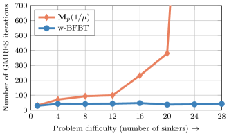
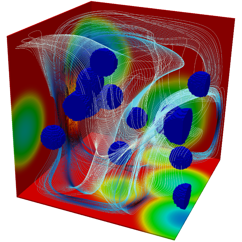
Figure 1: Left image shows the improvement in convergence obtained with the proposed w-BFBT preconditioner over a preconditioner using the inverse viscosity-weighted pressure mass matrix as Schur complement approximation. The number of randomly placed sinkers (high viscosity inclusions in low viscosity medium) increases along the horizontal axis. The vertical axis depicts the number of GMRES iterations required for $10^{6}$ residual reduction for the most popular $\mathbf{M}_{p}(1/\mu)$ and the proposed w-BFBT preconditioner. Fixed problem parameters are the dynamic ratio $\operatorname{DR}(\mu)=\max(\mu)/\!\min(\mu)=10^{8}$, discretization order $k=2$, and the mesh refinement level $\ell=7$, resulting in $128^{3}$ finite elements. Right image shows an example viscosity field with 16 sinkers (blue spheres depict highly viscous centers of Gaussian-like sinkers, low viscosity medium in red color) and the streamlines of the computed velocity field.

After defining a class of benchmark problems (Section 2.1), we compare the convergence obtained with different Schur complement approximations to motivate preconditioning with w-BFBT (Section 2.2). Theoretical estimates for spectral equivalence of w-BFBT are derived in Section 3. This is followed by a detailed numerical study showing when w-BFBT is advantageous over $\mathbf{M}_{p}(1/\mu)$ (Section 4), and a discussion of boundary modifications for w-BFBT that accelerate convergence (Section 5). In Section 6 we describe an algorithm for w-BFBT-based Stokes preconditioning, which uses hybrid spectral-geometric-algebraic multigrid (HMG). Finally, in Section 7, we provide numerical evidence for near-optimal algorithmic and parallel scalability. In particular, we demonstrate that the preconditioner’s parallel efficiency remains high when weak scaling out to tens of thousands of threads and even millions of threads.

To motivate our study of w-BFBT, we give an example for a possible improvement in convergence in Figure 1. There, a comparison is drawn between the $\mathbf{M}_{p}(1/\mu)$ and w-BFBT approximations for the Schur complement. The Stokes problem that is being solved is the multi-sinker benchmark problem from Section 2.1. The difficulty of the problem can be increased by adding more and more high-viscosity inclusions, called sinkers, into a low-viscosity background medium, which, as a result, introduces more variation in the viscosity. As can be seen in the figure, the number of GMRES iterations remain flat when preconditioning with w-BFBT, whereas the number of GMRES iterations increases significantly for higher sinker counts when using $\mathbf{M}_{p}(1/\mu)$, rendering $\mathbf{M}_{p}(1/\mu)$ inefficient for these types of difficult problems. Therefore we propose w-BFBT as an alternative Schur complement approximation for Stokes flow problems with a highly varying viscosity.

2 Benchmark problem and comparison of Schur complement approximations

This section further motivates the need for more effective Schur complement preconditioners. We first present a class of benchmark problems that range from relatively mild viscosity variations to highly heterogeneous. Then a challenging problem is used to compare Stokes solver convergence with different Schur complement approximations to demonstrate the limitations of established methods and motivate the development of w-BFBT.

2.1 Multi-sinker benchmark problem

The design of suitable benchmark problems is critical to conduct studies that can give useful convergence estimates for challenging applications. We seek complex geometrical structures in the viscosity that generate irregular, nonlocal, multiscale flow fields. Additionally, the viscosity should exhibit sharp gradients and its dynamic ratio $\operatorname{DR}(\mu)\coloneqq\max(\mu)/\!\min(\mu)$ (also commonly referred to as viscosity contrast) can be six orders of magnitude or higher in demanding applications. As in [29], we use a multi-sinker test problem with randomly positioned inclusions (e.g., as in Figure 1, right image) to study solver performance. We find that the arising viscosity structure is a suitable test for challenging, highly heterogeneous coefficient Stokes problems, and that the solver performance observed for such models can be indicative of the performance for other challenging applications.

In the (open) unit cube domain $\Omega=(0,1)^{3}$, we define the viscosity coefficient $\mu(\boldsymbol{x})\in[\mu_{\mathrm{min}},\mu_{\mathrm{max}}]$, $\boldsymbol{x}\in\Omega$, $0<\mu_{\mathrm{min}}<\mu_{\mathrm{max}}<\infty$, with dynamic ratio $\operatorname{DR}(\mu)=\mu_{\mathrm{max}}/\mu_{\mathrm{min}}$ by means of rescaling a $C^{\infty}$ indicator function $\chi_{n}(\boldsymbol{x})\in[0,1]$ that accumulates $n$ sinkers via a product of modified Gaussian functions:

$$\mu(\boldsymbol{x}) \coloneqq(\mu_{\mathrm{max}}-\mu_{\mathrm{min}})(1-\chi_{n}(\boldsymbol{x}))+\mu_{\mathrm{min}},\quad\boldsymbol{x}\in\Omega,$$

$$\chi_{n}(\boldsymbol{x}) \coloneqq\prod_{i=1}^{n}1-\exp\left(\!\!-\delta\max\left(0,\left|\boldsymbol{c}_{i}-\boldsymbol{x}\right|-\frac{\omega}{2}\right)^{2}\right),\quad\boldsymbol{x}\in\Omega,$$

where $\boldsymbol{c}_{i}\in\Omega$, $i=1,\ldots,n$, are the centers of the sinkers, $\delta>0$ controls the exponential decay of the Gaussian smoothing, and $\omega\geq 0$ is the diameter of a sinker where $\mu_{\mathrm{max}}$ is attained. Since all sinkers are equal in size, inserting more of them inside the domain will eventually result in overlapping with each other and possible intersections with the domain’s boundary. Throughout the paper, we fix $\delta=200$, $\omega=0.1$, and use the same set of precomputed random points $\boldsymbol{c}_{i}$ in all numerical experiments. Two parameters are varied: (i) the number of sinkers $n$ at random positions (the label S$n$-rand indicates a multi-sinker problem with $n$ randomly positioned sinkers) and (ii) the dynamic ratio $\operatorname{DR}(\mu)$ which in turn determines $\mu_{\mathrm{min}}\coloneqq\operatorname{DR}(\mu)^{-1/2}$ and $\mu_{\mathrm{max}}\coloneqq\operatorname{DR}(\mu)^{1/2}$. The right-hand side of (2), $\boldsymbol{f}(\boldsymbol{x})\coloneqq\left(0,0,\beta(\chi_{n}(\boldsymbol{x})-1)\right)$, $\beta=10$ constant, is such that it forces the high-viscosity sinkers downward, similarly to a gravity that pulls on high-density inclusions within a medium of lower density.

2.2 Comparison of Schur complement approximations

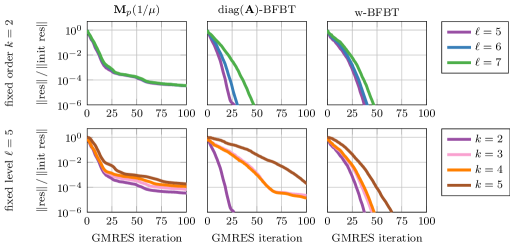
Figure 2: Comparison of Stokes solver convergence with $\mathbf{M}_{p}(1/\mu)$ (left column), $\operatorname{diag}(\mathbf{A})\text{-BFBT}$ (middle column), and w-BFBT (right column) preconditioning. We fix the problem S16-rand, $\operatorname{DR}(\mu)=10^{8}$ while varying mesh refinement level $\ell$ (top row) and discretization order $k$ (bottom row). This comparison shows that w-BFBT combines robust convergence of $\operatorname{diag}(\mathbf{A})\text{-BFBT}$ with improved algorithmic scalability when $k$ is increased.

We compare convergence of the Stokes solver using the Schur complement approximation $\mathbf{M}_{p}(1/\mu)$ with $\operatorname{diag}(\mathbf{A})\text{-BFBT}$ and with the proposed w-BFBT. The problem parameters are held fixed to S16-rand and $\operatorname{DR}(\mu)=10^{8}$. The numerical experiments are carried out using different levels of mesh refinement $\ell=5,\ldots,7$ (for fixed order $k=2$) and different discretization orders $k=2,\ldots,5$ (for fixed level $\ell=5$). A level $\ell$ corresponds to a mesh of $2^{3\ell}$ elements due to uniform refinement. Note that for these tests, the applications of $\mathbf{A}^{-1}$, $\left(\mathbf{B}\mathbf{C}_{w_{l}}^{-1}\mathbf{B}^{\mathsf{T}}\right)^{-1}$, and $\left(\mathbf{B}\mathbf{D}_{w_{r}}^{-1}\mathbf{B}^{\mathsf{T}}\right)^{-1}$ are approximated using a multigrid method (introduced in Section 6). These approximations are sufficiently accurate, such that the comparison is indicative of the effectiveness of the different Schur complement approximations. In particular, improving the approximation does not change the results, which are presented in Figure 2. In the left two plots, the poor Schur complement approximation by $\mathbf{M}_{p}(1/\mu)$ for this problem setup can be observed clearly. Convergence stagnates (similar results are found in [29, 36]).

Preconditioner $\operatorname{diag}(\mathbf{A})\text{-BFBT}$ (Figure 2, middle) is able to achieve fast convergence for discretization order $k=2$. A limitation of $\operatorname{diag}(\mathbf{A})\text{-BFBT}$ is a strong dependence on the order $k$. This can be explained by the decreasing diagonal dominance in the viscous block $\mathbf{A}$ with increasing order $k$: for higher $k$ the approximation of $\mathbf{A}$ by $\operatorname{diag}(\mathbf{A})$ deteriorates. Note that numerical experiments with $\mathbf{M}_{\boldsymbol{u}}\text{-BFBT}$ are not presented, because it performs poorly in the presence of spatially-varying viscosities. This leads to the conclusion that the choice of the weighting matrices $\mathbf{C}$, $\mathbf{D}$ in $\tilde{\mathbf{S}}_{\text{BFBT}}^{-1}$ crucially affects the quality of the Schur complement approximation.

The w-BFBT approximation delivers convergence that is nearly as fast as in the $\operatorname{diag}(\mathbf{A})\text{-BFBT}$, $k=2$ case, but without the severe deterioration when $k$ is increased (see Figure 2, right). Thus, w-BFBT exhibits the robustness of $\operatorname{diag}(\mathbf{A})\text{-BFBT}$ and additionally shows superior algorithmic scalability with respect to $k$. Having illustrated the efficacy of w-BFBT for certain problem parameters, we next establish spectral equivalence of w-BFBT (Section 3) and then analyze in more detail how crucial parameters influence convergence in Section 4.

3 Spectral equivalence of w-BFBT

Before we show spectral equivalence, we introduce notation and basic definitions.

3.1 Basic definitions

Let $\Omega\subset\mathbb{R}^{d}$ be a bounded domain with Lipschitz boundary $\partial\Omega$. We denote as $L^{2}(\Omega)$ the class of real-valued square-integrable functions, equipped with the usual $L^{2}$-inner product $\left(u\mathbin{,}v\right)_{L^{2}(\Omega)}$ and induced norm $\left\|u\right\|_{L^{2}(\Omega)}$, $u,v\in L^{2}(\Omega)$. We also consider corresponding spaces of $d$-dimensional vector-valued functions and $(d\times d)$-dimensional tensor-valued functions with component-wise multiplication, denoted by $L^{2}(\Omega)^{d}$ and $L^{2}(\Omega)^{d\times d}$. The subspace of $L^{2}(\Omega)$ that does not contain constant functions is denoted by $L^{2}(\Omega)/\mathbb{R}$. A bounded function, say $\alpha=\alpha(\boldsymbol{x})$, belongs to the space $L^{\infty}(\Omega)$ by satisfying the following finite norm: $\left\|\alpha\right\|_{L^{\infty}(\Omega)}\coloneqq\operatorname*{ess\,sup}_{\boldsymbol{x}\in\Omega}\left|\alpha(\boldsymbol{x})\right|<\infty$. We generalize the $L^{2}$-norms to classes of weighted $L^{2}_{\alpha}$-norms for functions $f\in L^{2}(\Omega)^{n}$, $n\in\{1,d,d\times d\}$, defined by

$$\left\|f\right\|_{L^{2}_{\alpha}(\Omega)^{n}}\coloneqq\left\|\alpha^{\frac{1}{2}}f\right\|_{L^{2}(\Omega)^{n}}\quad\text{for }\alpha\in L^{\infty}(\Omega)\text{, }0<\alpha(\boldsymbol{x})\text{ a.e.\ in }\Omega.$$

Next, we introduce $H^{m}(\Omega)$, with $m\geq 0$, which is the Sobolev space of $m$ derivatives in $L^{2}(\Omega)$, and for $m=1$ we use the inner product $\left(u\mathbin{,}v\right)_{H^{1}(\Omega)}\coloneqq\left(u\mathbin{,}v\right)_{L^{2}(\Omega)}+\left(\nabla u\mathbin{,}\nabla v\right)_{L^{2}(\Omega)},$ inducing the norm $\left\|u\right\|_{H^{1}(\Omega)}$. Functions in $H^{m}(\Omega)$ with vanishing trace on the boundary $\partial\Omega$ belong to the space $H^{m}_{0}(\Omega)$. Finally, we say that a function belongs to the class of $C^{\infty}(\Omega)$ if it has partial derivatives of any order in $\Omega$, and these derivatives are continuous.

We transition from abstract definitions to fluid mechanics. The differential operators acting on velocity $\boldsymbol{u}\in(H^{1}(\Omega))^{d}$ and pressure $p\in L^{2}(\Omega)$ within the Stokes equations are defined in the sense of distributions:

$$\nabla_{\!\mathrm{s}}\boldsymbol{u}\coloneqq\frac{1}{2}(\nabla\boldsymbol{u}+\nabla\boldsymbol{u}^{\mathsf{T}}),\quad B\boldsymbol{u}\coloneqq-\nabla\cdot\boldsymbol{u},\quad B^{\ast}p\coloneqq\nabla p.$$

Moreover, assume a sufficiently regular, bounded viscosity $\mu\in H^{1}(\Omega)\cap L^{\infty}(\Omega)$ such that $0<\mu_{\mathrm{min}}\leq\mu(\boldsymbol{x})$ a.e. in $\Omega$ and then define the viscous stress tensor $\boldsymbol{\tau}\coloneqq 2\mu\nabla_{\!\mathrm{s}}\boldsymbol{u}$. We denote the function space for velocity by

$$V\coloneqq\left\{\boldsymbol{u}\in(H^{1}(\Omega))^{d}\mid\boldsymbol{n}\cdot\boldsymbol{u}=0\text{ on }\partial\Omega\right\},$$ (9)

where $\boldsymbol{n}\in\mathbb{R}^{d}$ is the outward unit normal vector at the boundary $\partial\Omega$, and the function space for pressure by $Q\coloneqq L^{2}(\Omega)/\mathbb{R}$, and we introduce the viscous stress operator with a heterogeneous viscosity

$$A_{\mu}:V\rightarrow V^{\prime},\quad A_{\mu}\boldsymbol{u}\coloneqq-\nabla\cdot(2\mu\nabla_{\!\mathrm{s}}\boldsymbol{u})=-\nabla\cdot\boldsymbol{\tau}.$$

Given exterior forces acting on the fluid $\boldsymbol{f}\in V^{\prime}$, we consider the incompressible Stokes problem with free-slip and no-normal flow boundary conditions:

$$A_{\mu}\boldsymbol{u}+B^{\ast}p =\boldsymbol{f} \quad\text{in }\Omega,$$ (10a)

$$B\boldsymbol{u} =0 \quad\text{in }\Omega,$$ (10b)

$$\boldsymbol{T}\left[\boldsymbol{\tau}-p\mathbf{I}\right]\boldsymbol{n} =0 \quad\text{on }\partial\Omega,$$ (10c)

$$\boldsymbol{u}\cdot\boldsymbol{n} =0 \quad\text{on }\partial\Omega,$$ (10d)

in which we seek the velocity $\boldsymbol{u}\in V$ and pressure $p\in Q$. On the boundary, we have outward unit normal vectors $\boldsymbol{n}\in\mathbb{R}^{d}$ and tangential projectors $\boldsymbol{T}\coloneqq\mathbf{I}-\boldsymbol{n}\boldsymbol{n}^{\mathsf{T}}$. For the theoretical analysis sections, we altered the boundary conditions compared to (1c) to achieve a cleaner presentation.

For the definition of the w-BFBT approximation of the Schur complement, we introduce a Poisson operator for higher regularity pressure functions

$$K_{w}^{\ast}:H^{2}(\Omega)\rightarrow L^{2}(\Omega),\quad K_{w}^{\ast}p\coloneqq BwB^{\ast}p,$$ (11)

with an appropriate coefficient $w$ (see below) and augmented with homogeneous Neumann boundary conditions, $\boldsymbol{n}\cdot B^{\ast}p=0$. The $L^{2}$-adjoint of $K_{w}^{\ast}$ is denoted by $K_{w}$. Finally, we define the w-BFBT approximation of the Schur complement $S=BA_{\mu}^{-1}B^{\ast}$ by:

$$\tilde{S}_{\mathrm{w\text{-}BFBT}}\coloneqq K_{w_{r}}^{\ast}(Bw_{l}\,A_{\mu}\,w_{r}B^{\ast})^{-1}K_{w_{l}},$$ (12)

with sufficiently regular, bounded weight functions $w_{l},w_{r}\in H^{1}(\Omega)\cap L^{\infty}(\Omega)$ such that $0<w_{\mathrm{min}}\leq w_{l}(\boldsymbol{x}),w_{r}(\boldsymbol{x})$ a.e. in $\Omega$. Note that the definitions of the w-BFBT weight functions in the discrete case (8) are reciprocal to definitions in (11) and (12), because in the discrete case the weight functions were embedded into inverses of mass matrices.

3.2 Main theorem on spectral equivalence of w-BFBT

One measure for the efficacy of a preconditioner consists of the ratio of the maximal to minimal eigenvalues of the preconditioned system $\tilde{\mathbf{S}}_{\text{w-BFBT}}^{-1}\mathbf{S}$. This section establishes inequalities for spectral equivalence of w-BFBT by providing bounds on that ratio. The derivations are carried out in an infinite-dimensional setting. We begin by stating the main result of this section in Theorem 3.1 and continue with proving this result using a sequence of lemmas.

Theorem 3.1 (Main result).

Let $\hat{Q}=L^{2}(\Omega)/\mathbb{R}\cap H^{1}(\Omega)$. If the left and right w-BFBT weight functions are equal to

$$w_{l}(\boldsymbol{x})=\mu(\boldsymbol{x})^{-\frac{1}{2}}=w_{r}(\boldsymbol{x})\quad\text{for a.a. }\boldsymbol{x}\in\Omega,$$

then the exact Schur complement is equivalent to the w-BFBT approximation such that

$$\left(\tilde{S}_{\mathrm{w\text{-}BFBT}}\,q\mathbin{,}q\right)\leq\left(Sq\mathbin{,}q\right)\leq C_{\text{w-BFBT}}\left(\tilde{S}_{\mathrm{w\text{-}BFBT}}\,q\mathbin{,}q\right)\quad\text{for all }q\in\hat{Q},$$

where

$$C_{\text{w-BFBT}}\coloneqq\Bigl{(}1+\frac{1}{4}\left\|\nabla\mu\right\|_{L^{\infty}(\Omega)^{d}}^{2}\Bigr{)}\Bigl{(}C_{P,\mu}^{2}+1\Bigr{)}C_{K,\mu}^{2}$$

and the constants $C_{P,\mu},C_{K,\mu}>0$ stem from weighted Poincaré–Friedrichs’ and Korn’s inequalities, respectively (see Remark 3.7 for more information); the viscosity $\mu$ assumes the role of the weight function in the weighted inequalities.

If the viscosity and the w-BFBT weight functions are constant,

$$\mu\equiv 1,\quad w_{l}\equiv 1\equiv w_{r},$$

then the exact Schur complement is equivalent to the w-BFBT approximation such that

$$\left(\tilde{S}_{\mathrm{w\text{-}BFBT}}\,q\mathbin{,}q\right)\leq\left(Sq\mathbin{,}q\right)\leq(C_{P}^{2}+1)\,C_{K}^{2}\left(\tilde{S}_{\mathrm{w\text{-}BFBT}}\,q\mathbin{,}q\right)\quad\text{for all }q\in\hat{Q}$$

with constants $C_{P},C_{K}>0$ stemming from (the classical) Poincaré–Friedrichs’ and Korn’s inequalities, respectively.

3.3 Proofs

The proof of Theorem 3.1 is established in the remainder of this section. In what follows, suprema are understood over spaces excluding operator kernels that would cause a supremum to blow up. The following basic, but hereafter frequently used, result is shown for completeness of the discussion.

Lemma 3.2 (sup-form of inverse operator).

Let $V$ be a complete Hilbert space and $W\subseteq V$ be a dense subspace. Assume the linear operator $T:V\rightarrow V^{\prime}$ to be bounded, invertible, symmetric, and positive definite. Then for any $f\in V^{\prime}$ follows

$$\left(T^{-1}f\mathbin{,}f\right)=\sup_{w\in W}\frac{\left(w\mathbin{,}f\right)^{2}}{\left(Tw\mathbin{,}w\right)}.$$

Proof.

Let $w\in W$, then with Hölder’s inequality follows

$$\left(w\mathbin{,}f\right)^{2}=\left(T^{1/2}w\mathbin{,}T^{-1/2}f\right)^{2}\leq\left\|T^{1/2}w\right\|^{2}\left\|T^{-1/2}f\right\|^{2}=\left(Tw\mathbin{,}w\right)\left(T^{-1}f\mathbin{,}f\right).$$

Additionally, let $v=T^{-1}f$ and since $W\subseteq V$ dense, there exists a sequence $\{w_{k}\}_{k}\subset W$ such that $w_{k}\rightarrow v=T^{-1}f\in V$, hence

$$\frac{\left(w_{k}\mathbin{,}f\right)^{2}}{\left(Tw_{k}\mathbin{,}w_{k}\right)}\rightarrow\frac{\left(v\mathbin{,}f\right)^{2}}{\left(Tv\mathbin{,}v\right)}=\frac{\left(T^{-1}f\mathbin{,}f\right)^{2}}{\left(f\mathbin{,}T^{-1}f\right)}=\left(T^{-1}f\mathbin{,}f\right),$$

which shows that equality is achieved in the limit. ∎

The next lemma establishes Schur complement properties that are essential for deriving lower and upper bounds in the spectral equivalence estimates.

Lemma 3.3 (sup-form of Schur complement).

With the definitions from Section 3.1, the following two equalities hold:

$$\left(\tilde{S}_{\mathrm{w\text{-}BFBT}}\,q\mathbin{,}q\right)=\sup_{p\in\hat{P}}\frac{\left(B^{\ast}p\mathbin{,}w_{r}B^{\ast}q\right)^{2}}{\left(w_{l}A_{\mu}w_{r}B^{\ast}p\mathbin{,}B^{\ast}p\right)}\quad\text{for all }q\in\hat{Q},$$ (13)

where $\hat{P}\coloneqq C^{\infty}(\Omega)$ and $\hat{Q}\coloneqq L^{2}(\Omega)/\mathbb{R}\cap H^{1}(\Omega)$, and

$$\left(Sq\mathbin{,}q\right)=\sup_{\boldsymbol{v}\in V}\frac{\left(\boldsymbol{v}\mathbin{,}w_{r}B^{\ast}q\right)^{2}}{\left(w_{l}A_{\mu}w_{r}\boldsymbol{v}\mathbin{,}\boldsymbol{v}\right)}\quad\text{for all }q\in Q.$$ (14)

Proof.

For $q\in\hat{Q}$, we use integration by parts on the left hand side of (13) to obtain

$$\left(\tilde{S}_{\mathrm{w\text{-}BFBT}}\,q\mathbin{,}q\right) =\int_{\Omega}\left(w_{r}B^{\ast}(Bw_{l}A_{\mu}w_{r}B^{\ast})^{-1}K_{w_{l}}q\right)\left(B^{\ast}q\right)\,\mathrm{d}\boldsymbol{x}+b_{1}(q)$$

$$=\int_{\Omega}\left((Bw_{l}A_{\mu}w_{r}B^{\ast})^{-1}K_{w_{l}}q\right)\left(K_{w_{r}}q\right)\,\mathrm{d}\boldsymbol{x}+b_{1}(q)+b_{2}(q)$$

with boundary terms

$$b_{1}(q) \coloneqq-\int_{\partial\Omega}\left(\boldsymbol{n}\cdot w_{r}B^{\ast}(Bw_{l}A_{\mu}w_{r}B^{\ast})^{-1}K_{w_{l}}q\right)q\,\mathrm{d}\boldsymbol{x},$$

$$b_{2}(q) \coloneqq\int_{\partial\Omega}\left((Bw_{l}A_{\mu}w_{r}B^{\ast})^{-1}K_{w_{l}}q\right)\left(\boldsymbol{n}\cdot w_{r}B^{\ast}q\right)\,\mathrm{d}\boldsymbol{x}.$$

Using that $\hat{P}\subset H^{2}(\Omega)$ is dense, application of Lemma 3.2 and further integration by parts yields

$$\left(\tilde{S}_{\mathrm{w\text{-}BFBT}}\,q\mathbin{,}q\right) =\sup_{p\in\hat{P}}\frac{\left(p\mathbin{,}K_{w_{r}}q\right)^{2}}{\left(Bw_{l}A_{\mu}w_{r}B^{\ast}p\mathbin{,}p\right)}+b_{1}(q)+b_{2}(q)$$

$$=\sup_{p\in\hat{P}}\frac{\left(\left(B^{\ast}p\mathbin{,}w_{r}B^{\ast}q\right)+b_{3}(p,q)\right)^{2}}{\left(w_{l}A_{\mu}w_{r}B^{\ast}p\mathbin{,}B^{\ast}p\right)+b_{4}(p)}+b_{1}(q)+b_{2}(q)$$

with boundary terms

$$b_{3}(p,q) \coloneqq-\int_{\partial\Omega}p\left(\boldsymbol{n}\cdot w_{r}B^{\ast}q\right)\,\mathrm{d}\boldsymbol{x},$$

$$b_{4}(p) \coloneqq-\int_{\partial\Omega}\left(\boldsymbol{n}\cdot w_{l}A_{\mu}w_{r}B^{\ast}p\right)p\,\mathrm{d}\boldsymbol{x}.$$

Because the operator $K_{w_{r}}^{\ast}$ from (11) is augmented with homogeneous Neumann boundary conditions, $\boldsymbol{n}\cdot B^{\ast}p=0$, the boundary terms $b_{1}(q)$, $b_{2}(q)$, and $b_{3}(p,q)$ vanish. In addition, $p\in\hat{P}$ is sufficiently regular for the term $b_{4}(p)$ to be well-defined and it equals to zero because the velocity $\boldsymbol{u}$ satisfies $\boldsymbol{n}\cdot\boldsymbol{u}=0$ on $\partial\Omega$. Hence, (13) follows.

To show (14), let $q\in Q$, then for the exact Schur complement we apply integration by parts with a vanishing boundary term

$$\left(Sq\mathbin{,}q\right)=\left(BA_{\mu}^{-1}B^{\ast}q\mathbin{,}q\right)=\left(A_{\mu}^{-1}B^{\ast}q\mathbin{,}B^{\ast}q\right)=\left(w_{r}^{-1}A_{\mu}^{-1}w_{l}^{-1}w_{l}B^{\ast}q\mathbin{,}w_{r}B^{\ast}q\right)$$

and (14) follows from Lemma 3.2. ∎

A direct consequence of Lemma 3.3 is the following lower bound.

Corollary 3.4 (Lower bound, $\tilde{S}_{\mathrm{w\text{-}BFBT}}\lesssim S$).

The exact Schur complement is bounded by the w-BFBT approximation from below, i.e.,

$$\left(\tilde{S}_{\mathrm{w\text{-}BFBT}}\,q\mathbin{,}q\right)\leq\left(Sq\mathbin{,}q\right)\quad\text{for all }q\in\hat{Q},$$ (15)

where $\hat{Q}\coloneqq L^{2}(\Omega)/\mathbb{R}\cap H^{1}(\Omega)$.

Proof.

Let $\hat{P}=C^{\infty}(\Omega)$ and $q\in\hat{Q}$. Since $B^{\ast}$ maps $\hat{P}$ into $V$, we combine (13) and (14) to get

$$\left(\tilde{S}_{\mathrm{w\text{-}BFBT}}\,q\mathbin{,}q\right)=\sup_{p\in\hat{P}}\frac{\left(B^{\ast}p\mathbin{,}w_{r}B^{\ast}q\right)^{2}}{\left(w_{l}A_{\mu}w_{r}B^{\ast}p\mathbin{,}B^{\ast}p\right)}\leq\sup_{\boldsymbol{v}\in V}\frac{\left(\boldsymbol{v}\mathbin{,}w_{r}B^{\ast}q\right)^{2}}{\left(w_{l}A_{\mu}w_{r}\boldsymbol{v}\mathbin{,}\boldsymbol{v}\right)}=\left(Sq\mathbin{,}q\right),$$

and obtain the result (15). ∎

We begin the derivation of an upper bound for the case of constant viscosity $\mu\equiv 1$. Note that $\tilde{S}_{\mathrm{w\text{-}BFBT}}$ is scaling invariant with respect to constants multiplied to the w-BFBT weight functions $w_{l}$, $w_{r}$. Hence, it always assumes the correct scaling of $S$ independent of the viscosity constant. The result for constant viscosity presented below in Lemma 3.5 is generalized to variable viscosity in Lemma 3.6. While Lemma 3.5 is a special case of Lemma 3.6, we first prove the result for constant viscosity as the arguments are less technical and easier to follow. In the proof of the result for variable viscosity, we build on some of the arguments from the constant viscosity case and thus avoid unnecessary duplication.

Lemma 3.5 (Upper bound, $S\lesssim\tilde{S}_{\mathrm{w\text{-}BFBT}}$, for constant $\mu$).

Assume a constant viscosity $\mu\equiv 1$ and constant w-BFBT weight functions $w_{l}\equiv 1\equiv w_{r}$, and, as before in Lemma 3.3, let $\hat{Q}=L^{2}(\Omega)/\mathbb{R}\cap H^{1}(\Omega)$. Then the exact Schur complement is bounded by the w-BFBT approximation from above by

$$\left(Sq\mathbin{,}q\right)\leq(C_{P}^{2}+1)\,C_{K}^{2}\left(\tilde{S}_{\mathrm{w\text{-}BFBT}}\,q\mathbin{,}q\right)\quad\text{for all }q\in\hat{Q}$$ (16)

with constants $C_{P},C_{K}>0$ stemming from Poincaré–Friedrichs’ and Korn’s inequalities, respectively.

Proof.

Let $\hat{P}=C^{\infty}(\Omega)$ and $q\in\hat{Q}$, then due to (13) we can write

$$\left(\tilde{S}_{\mathrm{w\text{-}BFBT}}\,q\mathbin{,}q\right)=\sup_{p\in\hat{P}}\frac{\left(B^{\ast}p\mathbin{,}B^{\ast}q\right)^{2}}{\left\|B^{\ast}p\right\|_{(H^{1}(\Omega))^{d}}^{2}}\,\frac{\left\|B^{\ast}p\right\|_{(H^{1}(\Omega))^{d}}^{2}}{\left(A_{1}B^{\ast}p\mathbin{,}B^{\ast}p\right)}.$$ (17)

To estimate the second factor on the right-hand side of (17), note that

$$\left(A_{1}B^{\ast}p\mathbin{,}B^{\ast}p\right)=2\left(\nabla_{\!\mathrm{s}}B^{\ast}p\mathbin{,}\nabla_{\!\mathrm{s}}B^{\ast}p\right)=2\left(\nabla B^{\ast}p\mathbin{,}\nabla B^{\ast}p\right)=2\left\|\nabla B^{\ast}p\right\|_{(L^{2}(\Omega))^{d\times d}}^{2},$$

where we used that $\boldsymbol{n}\cdot B^{\ast}p=0$ on the boundary and that $\nabla B^{\ast}p$ is symmetric. Thus,

$$\left(A_{1}B^{\ast}p\mathbin{,}B^{\ast}p\right)\leq 2\left\|B^{\ast}p\right\|_{(H^{1}(\Omega))^{d}}^{2}.$$ (18)

For the first factor on the right-hand side of (17), observe that for any $\boldsymbol{v}\in V$ there exists a sequence $\{p_{i}\}_{i}\subset\hat{P}\subset H^{2}(\Omega)$ such that $K_{1}^{\ast}p_{i}=BB^{\ast}p_{i}\rightarrow B\boldsymbol{v}$, since $K_{1}^{\ast}$ is invertible, where convergence is with respect to the $L^{2}$-norm. Thus,

$$\sup_{p\in\hat{P}}\frac{\left(B^{\ast}p\mathbin{,}B^{\ast}q\right)}{\left\|B^{\ast}p\right\|_{(H^{1}(\Omega))^{d}}}=\sup_{\boldsymbol{v}\in V}\frac{\left(\boldsymbol{v}\mathbin{,}B^{\ast}q\right)}{\left\|\boldsymbol{v}\right\|_{(H^{1}(\Omega))^{d}}}=\left\|B^{\ast}q\right\|_{(H^{-1}(\Omega))^{d}}.$$ (19)

Combining (18) and (19) provides the following estimate for the w-BFBT Schur complement approximation (17):

$$\left(\tilde{S}_{\mathrm{w\text{-}BFBT}}\,q\mathbin{,}q\right)\geq\frac{1}{2}\left\|B^{\ast}q\right\|_{(H^{-1}(\Omega))^{d}}^{2}.$$ (20)

The exact Schur complement, on the other hand, in the form (14) from Lemma 3.3, can be bounded by

$$\left(Sq\mathbin{,}q\right)=\sup_{\boldsymbol{v}\in V}\frac{\left(\boldsymbol{v}\mathbin{,}B^{\ast}q\right)^{2}}{\left(A_{1}\boldsymbol{v}\mathbin{,}\boldsymbol{v}\right)}\leq\sup_{\boldsymbol{v}\in V}\frac{\left\|\boldsymbol{v}\right\|_{(H^{1}(\Omega))^{d}}^{2}\left\|B^{\ast}q\right\|_{(H^{-1}(\Omega))^{d}}^{2}}{2\left\|\nabla_{\!\mathrm{s}}\boldsymbol{v}\right\|_{(L^{2}(\Omega))^{d\times d}}^{2}}.$$ (21)

With Poincaré–Friedrichs’ inequality,

$$\left\|\boldsymbol{v}\right\|_{L^{2}(\Omega)^{d}}\leq C_{P}\left\|\nabla\boldsymbol{v}\right\|_{(L^{2}(\Omega))^{d\times d}},$$

where the constant $C_{P}>0$ depends on the domain $\Omega$, and Korn’s inequality,

$$\left\|\nabla\boldsymbol{v}\right\|_{(L^{2}(\Omega))^{d\times d}}\leq C_{K}\left\|\nabla_{\!\mathrm{s}}\boldsymbol{v}\right\|_{(L^{2}(\Omega))^{d\times d}},$$

with constant $C_{K}>0$, we obtain

$$\frac{1}{(C_{P}^{2}+1)}\left\|\boldsymbol{v}\right\|_{(H^{1}(\Omega))^{d}}^{2}\leq\left\|\nabla\boldsymbol{v}\right\|_{(L^{2}(\Omega))^{d\times d}}^{2}\leq C_{K}^{2}\left\|\nabla_{\!\mathrm{s}}\boldsymbol{v}\right\|_{(L^{2}(\Omega))^{d\times d}}^{2},$$

and substituting this into (21) gives

$$\left(Sq\mathbin{,}q\right)\leq\frac{(C_{P}^{2}+1)\,C_{K}^{2}}{2}\left\|B^{\ast}q\right\|_{(H^{-1}(\Omega))^{d}}^{2}.$$ (22)

Together with (20), this yields the desired result (16). ∎

We complete the presentation of spectral equivalence by deriving an upper bound for problems with variable viscosities.

Lemma 3.6 (Upper bound, $S\lesssim\tilde{S}_{\mathrm{w\text{-}BFBT}}$, for variable $\mu$).

As before in Lemma 3.3, let $\hat{Q}=L^{2}(\Omega)/\mathbb{R}\cap H^{1}(\Omega)$. If the left and right w-BFBT weight functions are equal to

$$w_{l}(\boldsymbol{x})=\mu(\boldsymbol{x})^{-\frac{1}{2}}=w_{r}(\boldsymbol{x})\quad\text{for a.a. }\boldsymbol{x}\in\Omega,$$ (23)

then the exact Schur complement is bounded by the w-BFBT approximation from above by

$$\left(Sq\mathbin{,}q\right)\leq\Bigl{(}1+\frac{1}{4}\left\|\nabla\mu\right\|_{L^{\infty}(\Omega)^{d}}^{2}\Bigr{)}\Bigl{(}C_{P,\mu}^{2}+1\Bigr{)}C_{K,\mu}^{2}\left(\tilde{S}_{\mathrm{w\text{-}BFBT}}\,q\mathbin{,}q\right)\quad\text{for all }q\in\hat{Q}$$ (24)

with constants $C_{P,\mu},C_{K,\mu}>0$ stemming from weighted Poincaré–Friedrichs’ and Korn’s inequalities, respectively, where $\mu$ assumes the role of the weight function.

Proof.

Let the weight functions be equal, $w_{l}\equiv w\equiv w_{r}$, but (for now) otherwise arbitrary subject to the condition $0<w_{\mathrm{min}}\leq w(\boldsymbol{x})$ for a.a. $\boldsymbol{x}\in\Omega$. At the end of this proof we will argue the special role of the choice (23) for the weight functions. In addition, let $\hat{P}=C^{\infty}(\Omega)$ and $q\in\hat{Q}$, then due to (13) we can write

$$\left(\tilde{S}_{\mathrm{w\text{-}BFBT}}\,q\mathbin{,}q\right)=\sup_{p\in\hat{P}}\frac{\left(B^{\ast}p\mathbin{,}wB^{\ast}q\right)^{2}}{\left\|B^{\ast}p\right\|_{(H^{1}(\Omega))^{d}}^{2}}\,\frac{\left\|B^{\ast}p\right\|_{(H^{1}(\Omega))^{d}}^{2}}{\left(wA_{\mu}wB^{\ast}p\mathbin{,}B^{\ast}p\right)}.$$ (25)

We begin by estimating the second factor on the right-hand side of (25). For an arbitrary $\boldsymbol{v}\in(H^{1}(\Omega))^{d}$, observe that $\nabla_{\!\mathrm{s}}(w\boldsymbol{v})=w\nabla_{\!\mathrm{s}}\boldsymbol{v}+\nabla w\otimes\boldsymbol{v},$ where “$\otimes$” denotes the outer product of two vectors in $\mathbb{R}^{d}$, and thus

$$\left(wA_{\mu}w\boldsymbol{v}\mathbin{,}\boldsymbol{v}\right)=2\left(\mu\nabla_{\!\mathrm{s}}(w\boldsymbol{v})\mathbin{,}\nabla_{\!\mathrm{s}}(w\boldsymbol{v})\right)=2\left\|\sqrt{\mu}w\nabla_{\!\mathrm{s}}\boldsymbol{v}+\sqrt{\mu}\nabla w\otimes\boldsymbol{v}\right\|_{(L^{2}(\Omega))^{d\times d}}^{2}.$$

Applying the triangle inequality and then Hölder’s inequality to the resulting terms,

$$\left\|\sqrt{\mu}w\nabla_{\!\mathrm{s}}\boldsymbol{v}\right\|_{(L^{2}(\Omega))^{d\times d}}^{2} \leq\left\|\sqrt{\mu}w\right\|_{L^{\infty}(\Omega)}^{2}\left\|\nabla_{\!\mathrm{s}}\boldsymbol{v}\right\|_{(L^{2}(\Omega))^{d\times d}}^{2},$$

$$\left\|\sqrt{\mu}\nabla w\otimes\boldsymbol{v}\right\|_{(L^{2}(\Omega))^{d\times d}}^{2} \leq\left\|\sqrt{\mu}\nabla w\right\|_{L^{\infty}(\Omega)^{d}}^{2}\left\|\boldsymbol{v}\right\|_{L^{2}(\Omega)^{d}}^{2},$$

and thus we obtain the estimate

$$\left(wA_{\mu}w\boldsymbol{v}\mathbin{,}\boldsymbol{v}\right)\leq 2C_{A,\mu,w}\left\|\boldsymbol{v}\right\|_{(H^{1}(\Omega))^{d}}^{2},$$

where

$$C_{A,\mu,w}\coloneqq\left\|\sqrt{\mu}w\right\|_{L^{\infty}(\Omega)}^{2}+\left\|\sqrt{\mu}\nabla w\right\|_{L^{\infty}(\Omega)^{d}}^{2}.$$ (26)

Similarly to (19) and (20), we obtain the following estimate for the w-BFBT Schur complement approximation (25):

$$\left(\tilde{S}_{\mathrm{w\text{-}BFBT}}\,q\mathbin{,}q\right)\geq\frac{1}{2C_{A,\mu,w}}\left\|wB^{\ast}q\right\|_{(H^{-1}(\Omega))^{d}}^{2}.$$ (27)

Proceeding with the exact Schur complement, we obtain from (14) in Lemma 3.3 that

$$\left(Sq\mathbin{,}q\right)=\sup_{\boldsymbol{v}\in V}\frac{\left(w^{-1}\boldsymbol{v}\mathbin{,}wB^{\ast}q\right)^{2}}{\left(A_{\mu}\boldsymbol{v}\mathbin{,}\boldsymbol{v}\right)}\leq\sup_{\boldsymbol{v}\in V}\frac{\left\|w^{-1}\boldsymbol{v}\right\|_{(H^{1}(\Omega))^{d}}^{2}\left\|wB^{\ast}q\right\|_{(H^{-1}(\Omega))^{d}}^{2}}{2\left\|\sqrt{\mu}\nabla_{\!\mathrm{s}}\boldsymbol{v}\right\|_{(L^{2}(\Omega))^{d\times d}}^{2}}.$$ (28)

We require a weighted Poincaré–Friedrichs’ inequality (see Remark 3.7 for details),

$$\left\|\boldsymbol{v}\right\|_{L^{2}_{w^{-2}}(\Omega)^{d}}\leq C_{P,w^{-2}}\left\|\nabla\boldsymbol{v}\right\|_{L^{2}_{w^{-2}}(\Omega)^{d\times d}},$$ (29)

and also a weighted Korn’s inequality (see Remark 3.7 for more information),

$$\left\|\nabla\boldsymbol{v}\right\|_{L^{2}_{\mu}(\Omega)^{d\times d}}\leq C_{K,\mu}\left\|\nabla_{\!\mathrm{s}}\boldsymbol{v}\right\|_{L^{2}_{\mu}(\Omega)^{d\times d}}.$$ (30)

With (29) and (30), we are able to bound (28) from above:

$$\left(Sq\mathbin{,}q\right)\leq\frac{\Bigl{(}C_{P,w^{-2}}^{2}+1\Bigr{)}C_{K,\mu}^{2}}{2}\left(\sup_{\boldsymbol{v}\in V}\frac{\left\|\nabla\boldsymbol{v}\right\|_{L^{2}_{w^{-2}}(\Omega)^{d\times d}}}{\left\|\nabla\boldsymbol{v}\right\|_{(L^{2}_{\mu}(\Omega))^{d\times d}}}\right)\left\|wB^{\ast}q\right\|_{(H^{-1}(\Omega))^{d}}^{2}.$$ (31)

The supremum term in (31) and the constant $C_{A,\mu,w}$ in (26) motivate the choice for the weight $w$ to be

$$w\coloneqq\mu^{-\frac{1}{2}}.$$

Then the supremum in (31) vanishes and (26) simplifies to

$$C_{A,\mu,w}=1+\frac{1}{4}\left\|\nabla\mu\right\|_{L^{\infty}(\Omega)^{d}}^{2}.$$

Substituting this into (27) together with inequality (31) yields the desired result (24). ∎

Remark 3.7.

In the proof of Lemma 3.6 we utilized a weighted Poincaré–Friedrichs’ inequality, for which the optimal constant is

$$C_{P,\mu}=\sup_{\boldsymbol{v}\in V}\frac{\left\|\boldsymbol{v}\right\|_{L^{2}_{\mu}(\Omega)^{d}}}{\left\|\nabla\boldsymbol{v}\right\|_{L^{2}_{\mu}(\Omega)^{d\times d}}},$$

where the viscosity takes the role of the weight function. While weighted Poincaré and Friedrichs’ inequalities have been investigated in the literature numerous times, usually they are proven by contradiction and scaling arguments, which does not provide information about the constants. If explicit constants are found, they depend, in general, on the weight such that the resulting estimates are too pessimistic, e.g., $C_{P,\mu}=\mathcal{O}(\operatorname{DR}(\mu))$. Knowledge of constants that are robust with respect to weight functions is limited. In the context of a posteriori error estimates for finite elements, weight-independent constants could be found for convex domains and weights that are a positive power of a non-negative concave function [10]. These results were refined for star-shaped domains under certain assumptions for the weights [42]. For another class of weights, namely quasi-monotone piecewise constant weight functions, robust constants were derived in [33].

In addition to weighted Poincaré–Friedrichs’, we utilized a weighted Korn’s inequality in the proof of Lemma 3.6. The optimal constant for this inequality is

$$C_{K,\mu}=\sup_{\boldsymbol{v}\in V}\frac{\left\|\nabla\boldsymbol{v}\right\|_{L^{2}_{\mu}(\Omega)^{d\times d}}}{\left\|\nabla_{\!\mathrm{s}}\boldsymbol{v}\right\|_{L^{2}_{\mu}(\Omega)^{d\times d}}}.$$

As for $C_{P,\mu}$, straightforward estimation results in an overly pessimistic weight-dependent constant, namely $C_{K,\mu}=\mathcal{O}(\operatorname{DR}(\mu))$, [25]. Other work utilizing weighted Korn’s inequalities usually aims to derive inequalities for special domain shapes, e.g., [1].

In summary, robust constants for weighted Poincaré–Friedrichs’ and Korn’s inequalities for general weight functions are difficult to obtain and limitations exist in the form of assumptions on the weights. Further work on this topic could improve the constants for the spectral equivalence of w-BFBT but is beyond the scope of this paper.

4 Robustness of w-BFBT

In this section, we analyze the robustness properties of the widely used Schur complement approximation $\mathbf{M}_{p}(1/\mu)$ and the new w-BFBT via numerical experiments. Furthermore, we calculate the spectra for both approaches and thus support the discussion in Section 3 about theoretical eigenvalue bounds with numerical results. The comparison of $\mathbf{M}_{p}(1/\mu)$ and w-BFBT is of particular importance, because of the widespread use of the inverse viscosity-weighted mass matrix. It is therefore of interest to determine when convergence with $\mathbf{M}_{p}(1/\mu)$ deteriorates and using w-BFBT becomes beneficial. A comparison with $\operatorname{diag}(\mathbf{A})\text{-BFBT}$ was not performed because Section 2.2 already showed that $\operatorname{diag}(\mathbf{A})\text{-BFBT}$ performs similarly or worse than w-BFBT, hence there are no advantages in using $\operatorname{diag}(\mathbf{A})\text{-BFBT}$ over w-BFBT.

For the numerical experiments in this section, we return to the definitions and setup from Section 2.1. To apply the inverse of $\mathbf{M}_{p}(1/\mu)$, we diagonalize the mass matrix of the discontinuous, modal pressure space by forming its lumped version (4). Moreover, to apply the approximate inverse of the viscous block in (3) we use the same multigrid method for each of the two Schur approximations; this multigrid method is also used for the inverse operators of w-BFBT in (8). The details of the multigrid method are provided in Section 6. To compare the robustness, we vary two problem parameters: (i) the number of randomly placed sinkers $n$ and (ii) the dynamic ratio $\operatorname{DR}(\mu)$. The parameter $n$ influences the geometric complexity of the viscosity $\mu$ while $\operatorname{DR}(\mu)$ controls the magnitude of viscosity gradients.

Tables 1(a) and 1(b) present the number of GMRES iterations for a $10^{-6}$ residual reduction in the Euclidean norm. Observe that for the S1-rand problem, the iteration count is essentially the same for both $\mathbf{M}_{p}(1/\mu)$ and w-BFBT, and that it stays stable across all dynamic ratios $\operatorname{DR}(\mu)=10^{4},\ldots,10^{10}$. Hence for this simple problem, w-BFBT has no advantages and its additional computational cost makes it less efficient than $\mathbf{M}_{p}(1/\mu)$. However, the limitations of the $\mathbf{M}_{p}(1/\mu)$ approach become apparent by increasing the number of randomly positioned sinkers. Two observations for $\mathbf{M}_{p}(1/\mu)$ can be made from Table 1(a). First, the number of GMRES iterations rises with increasing number of sinkers (factor $\sim$80 increase for $n=1,\ldots,28$, $\operatorname{DR}(\mu)=10^{8}$). Second, in a multi-sinker setup the dependence on $\operatorname{DR}(\mu)$ becomes more severe (factor $\sim$50 increase for $n=24$, $\operatorname{DR}(\mu)=10^{4},\ldots,10^{10}$). This demonstrates that $\mathbf{M}_{p}(1/\mu)$ is a poor approximation of the Schur complement for certain classes of problems with highly heterogeneous viscosities.

The advantages in robustness of the w-BFBT preconditioner are demonstrated in Table 1(b). Compared to $\mathbf{M}_{p}(1/\mu)$, the number of GMRES iterations is stable and the increase over the whole range of problem parameters is just a factor of 2. Only 60 iterations are needed for the most extreme problem, namely S28-rand, $\operatorname{DR}(\mu)=10^{10}$, for which convergence with $\mathbf{M}_{p}(1/\mu)$ essentially stagnated.

Table 1: Robustness classification for Schur complement approximations 1(a) $\mathbf{M}_{p}(1/\mu)$ and 1(b) w-BFBT in terms of number of GMRES iterations ($10^{-6}$ residual reduction, GMRES restart every $100$ iterations). Number of randomly placed sinkers (#sinkers) is increased across rows, while dynamic ratio ($\operatorname{DR}(\mu)$) is increased across columns. Discretization is fixed at $k=2$, $\ell=7$.

(a) $\mathbf{M}_{p}(1/\mu)$

$\#\text{sinkers}\setminus\operatorname{DR}(\mu)$	$10^{4}$	$10^{6}$	$10^{8}$	$10^{10}$
S1-rand	29	31	31	29
S4-rand	53	63	71	80
S8-rand	64	79	93	165
S12-rand	70	86	99	180
S16-rand	85	167	231	891
S20-rand	84	167	380	724
S24-rand	117	286	3279	5983
S28-rand	108	499	2472	$>$10000

(b) w-BFBT

$\#\text{sinkers}\setminus\operatorname{DR}(\mu)$	$10^{4}$	$10^{6}$	$10^{8}$	$10^{10}$
S1-rand	29	29	29	30
S4-rand	39	41	42	44
S8-rand	38	40	41	44
S12-rand	38	40	43	45
S16-rand	40	45	47	48
S20-rand	34	36	37	38
S24-rand	31	32	39	55
S28-rand	29	31	42	60

More insight concerning the different convergence behaviors can be gained from the eigenvalues in Figure 3. The plots in that figure are for two-dimensional multi-sinker problems, which are analogous to the three-dimensional benchmark problems from Section 2.1. We discretize the problems on triangular meshes utilizing the FEniCS library [28]. We choose $\mathbb{P}_{2}^{\mathrm{bubble}}\times\mathbb{P}_{1}^{\mathrm{disc}}$ finite elements [11, 12] because they represent a close analog to the $\mathbb{Q}_{2}\times\mathbb{P}_{1}^{\mathrm{disc}}$ elements, which are employed on (three-dimensional) hexahedral meshes. Each plot shows the eigenvalues of the exact Schur complement and the eigenvalues of the preconditioned Schur complement for the $\mathbf{M}_{p}(1/\mu)$ and w-BFBT approximations, where all inverse matrices, e.g., the viscous block matrix $\mathbf{A}$ and the pressure Poisson matrices within w-BFBT, are inverted with a direct solver. Effective preconditioners exhibit a strong clustering of eigenvalues, whereas the convergence of Krylov methods deteriorates if the eigenvalues are spread out. We recognize different characteristics in the spectra associated with $\mathbf{M}_{p}(1/\mu)$ and w-BFBT preconditioning. For $\mathbf{M}_{p}(1/\mu)$, the dominant eigenvalues are clustered around one while smaller eigenvalues, i.e., eigenvalues $\ll 1$, are spread out. The behavior for w-BFBT is the opposite: the dominant eigenvalues are spread out and the smaller eigenvalues are tightly clustered around one. Now, as the problem difficulty is increased by introducing more viscosity anomalies in the domain, the spreading of smaller eigenvalues associated with $\mathbf{M}_{p}(1/\mu)$ becomes more severe (compare in Figure 3 the top row of plots and the bottom row of plots). We postulate that this is the property that is responsible for the deteriorating convergence with $\mathbf{M}_{p}(1/\mu)$ that was observed in Table 1(a). With w-BFBT on the other hand, the spectrum remains largely unaffected by increased sinker counts. The clustering of smaller eigenvalues around one remains stable, which is likely the reason for the robustness of w-BFBT. The lower bound on the eigenvalues that we observe here numerically supports the theoretical estimates on spectral equivalence in Section 3. Therefore we find the lower bound to be sharp and, moreover, to be essential for the robustness of the w-BFBT preconditioner.

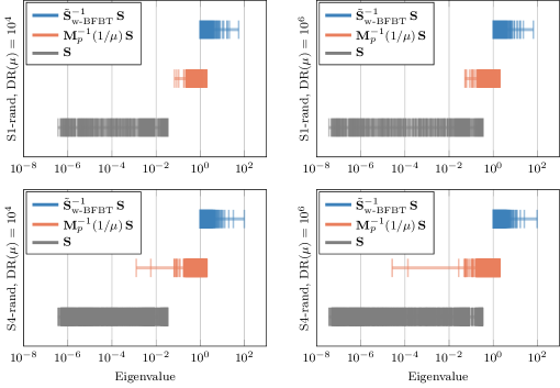
Figure 3: Spectra of the Schur complement (gray), $\mathbf{M}_{p}(1/\mu)$-preconditioned Schur complement (red), and w-BFBT-preconditioned Schur complement (blue); zero eigenvalues corresponding to the null space of the Schur complement matrix are omitted. Results for viscosities with one sinker (S1-rand) are shown in top row, and with four sinkers (S4-rand) in the bottom row of plots; $\operatorname{DR}(\mu)=10^{4}$ in the left column and $\operatorname{DR}(\mu)=10^{6}$ in the right column. The two-dimensional Stokes equations are discretized with $\mathbb{P}_{2}^{\mathrm{bubble}}\times\mathbb{P}_{1}^{\mathrm{disc}}$ finite elements on a uniform triangular mesh consisting of 512 triangles using the FEniCS library. As the problem difficulty increases from one to four sinkers, the spreading of small eigenvalues for $\mathbf{M}_{p}(1/\mu)$ becomes more severe, which is disadvantageous for solver convergence. For w-BFBT, the spectrum remains largely unaffected by increased sinker counts, which contributes to convergence that is robust with respect to viscosity variations.

Remark 4.1.

In addition to the $\mathbb{P}_{2}^{\mathrm{bubble}}\times\mathbb{P}_{1}^{\mathrm{disc}}$ discretization used for the results in Figure 3, we also calculated the spectra using $\mathbb{P}_{2}\times\mathbb{P}_{1}$ Taylor-Hood finite elements. We obtained very similar results for this discretization, which uses continuous elements to approximate the pressure. Therefore, both the efficacy of w-BFBT as a preconditioner and the issues with $\mathbf{M}_{p}(1/\mu)$ seem to be largely unaffected by the specific type of discretization, at least for the two cases that we tested.

Remark 4.2.

The convergence of the Stokes solver with the $\mathbf{M}_{p}(1/\mu)$ preconditioner can be improved by approximating the heterogeneous viscosity $\mu(\boldsymbol{x})$ with elementwise constants, computed by averaging $\mu$ over each element [3]. The benefit of faster convergence comes at the cost of slower asymptotic convergence of the discrete finite element solution and an altered constitutive relationship, which might be a less accurate representation of the physics; this is, however, problem-dependent. Moreover, for a nonlinear (e.g., power-law) rheology, elementwise averaging of $\mu$ can introduce non-physical, artificial disturbances in the effective viscosity during Newton or Picard-type nonlinear solves. We observed such a behavior in mantle convection simulations, which are governed by a nonlinear power-law rheology. Here, viscosity averaging led to non-physical checkerboard-like patterns upon convergence of the nonlinear Newton solver.

Remark 4.3.

In practice, the convergence of w-BFBT can be improved for coarse meshes, where the viscosity variations over elements are large. This is achieved by alternative choices for the diagonal weighting matrices $\mathbf{C}_{w_{l}}$ and $\mathbf{D}_{w_{r}}$ from (8) with the weights

$$w_{l}(\boldsymbol{x})=\left(\mu^{2}(\boldsymbol{x})+\left|\nabla\mu(\boldsymbol{x})\right|^{2}\right)^{\frac{1}{4}}=w_{r}(\boldsymbol{x})\quad\text{for all }\boldsymbol{x}\in\Omega,$$

where $\left|\cdot\right|$ denotes the Euclidean norm in $\mathbb{R}^{d}$. These viscosity gradient-based w-BFBT weights have the advantage of performing at least as well as the pure viscosity-based weights proposed in Section 1.3, but they exhibit superior robustness on coarser meshes. They are, however, challenging to analyze theoretically.

5 Modifications for Dirichlet boundary conditions

In Section 2.2, deteriorating approximation properties of w-BFBT for increasing discretization order and mesh refinement level could be observed. The numerical experiments in Figure 2, right did show slightly slower convergence when $k$ and $\ell$ were increased. This can stem from w-BFBT representing a poor approximation to the exact Schur complement at the boundary $\partial\Omega$ in the presence of Dirichlet boundary conditions for the velocity. This section investigates modifications to w-BFBT near a Dirichlet boundary and aims at obtaining mesh independence and only a mild dependence on discretization order in terms of Stokes solver convergence.

Consider the commutator that leads to the w-BFBT formulation in an infinite-dimensional form: $AB^{\ast}-B^{\ast}X\approx 0$, where $A$ represents the viscous stress operator, $B^{\ast}$ the gradient operator and $X$ the sought commuting operator. In case of an unbounded domain $\Omega=\mathbb{R}^{d}$ and constant viscosity $\mu\equiv 1$, this commutator is exactly satisfied since $(\nabla\cdot\nabla)\nabla-\nabla(\nabla\cdot\nabla)=0$. For Dirichlet boundary conditions, the commutator does not, in general, vanish at the boundary. Therefore a possible source for deteriorating Schur complement approximation properties of w-BFBT is a commutator mismatch for mesh elements that are touching the boundary $\partial\Omega$. A similar observation was also made in [17, 16]. A possible remedy is to modify the norm in the least-squares minimization problem (6), which is represented by the matrix $\mathbf{C}^{-1}$, such that a damping factor is applied to the matrix entries near the boundary. By damping the influence of the boundary in the minimization objective, more emphasis is given to the domain interior, and the w-BFBT approximation is improved.

Damping near Dirichlet boundaries can be incorporated by modifying the matrices $\mathbf{C}_{w_{l}}^{-1}$ or $\mathbf{D}_{w_{r}}^{-1}$ of the w-BFBT inverse Schur complement approximation (8). A similar idea for BFBT in a Navier–Stokes setting is presented in [17], where a damping to the weighting matrix $\mathbf{D}^{-1}$ in (7) is introduced to achieve mesh independence ($\mathbf{C}^{-1}$ is not changed). There, damping affects the normal components of the velocity space inside mesh elements touching $\partial\Omega$ and simply a constant damping factor of $1/10$ is set regardless of mesh refinement $\ell$. Also, only the discretization order $k=2$ was considered (in addition to $\mathbb{Q}_{2}\times\mathbb{Q}_{1}$ and MAC discretizations).

Now, we attempt to enhance our understanding of how modifications at a Dirichlet boundary $\partial\Omega$ influence convergence and therefore the efficacy of w-BFBT as a Schur complement approximation. Let $\Omega_{D}\coloneqq\bigcup_{e\in D}\Omega_{e}$, $D\coloneqq\{e\mid\overline{\Omega_{e}}\cap\partial\Omega\neq\emptyset\}$ be the set of all mesh elements $\Omega_{e}$ touching the Dirichlet boundary. Given values $a_{l},a_{r}\geq 1$, extend the previous definition of the weights $w_{l}=w_{r}=\sqrt{\mu}$ (see Section 1.3) to a version with boundary modification:

$$w_{l}(\boldsymbol{x})\coloneqq\begin{cases}a_{l}\sqrt{\mu(\boldsymbol{x})}&\boldsymbol{x}\in\Omega_{D},\\ \sqrt{\mu(\boldsymbol{x})}&\boldsymbol{x}\notin\Omega_{D},\end{cases}\quad\text{and}\quad w_{r}(\boldsymbol{x})\coloneqq\begin{cases}a_{r}\sqrt{\mu(\boldsymbol{x})}&\boldsymbol{x}\in\Omega_{D},\\ \sqrt{\mu(\boldsymbol{x})}&\boldsymbol{x}\notin\Omega_{D}.\end{cases}$$ (32)

We obtain matrices $\mathbf{C}_{w_{l}}=\tilde{\mathbf{M}}_{\boldsymbol{u}}(w_{l})$ and $\mathbf{D}_{w_{r}}=\tilde{\mathbf{M}}_{\boldsymbol{u}}(w_{r})$ in (8) that may differ at boundary elements in $\Omega_{D}$ due to possibly different values for $a_{l}$ and $a_{r}$. Note that amplifying the weight functions $w_{l}$, $w_{r}$ at the boundary is similar to damping at the boundary after taking the inverses $\mathbf{C}_{w_{l}}^{-1}$, $\mathbf{D}_{w_{r}}^{-1}$.

The Stokes solver convergence under the influence of boundary amplifications $a_{l}$, $a_{r}$ is summarized in Table 2. The table shows that the boundary amplification is most effective when performed non-symmetrically, i.e., either $a_{l}>1$ or $a_{r}>1$ but not both. Further, we deduce that with higher mesh refinement level $\ell$, the boundary amplification should increase roughly proportional to $2^{\ell}$ (or proportional to the reciprocal element size, here $h^{-1}=2^{\ell}$). Similar observations can be made for the discretization order $k$, i.e., amplification needs to increase for larger $k$ to avoid higher iteration counts. These implications were made based on extensive numerical experiments for which Table 2 serves as a representative summary.

Table 2: Influence of boundary modification factors $a_{l}$, $a_{r}$ on the Stokes solver convergence with w-BFBT for discretizations: $k=2$, $\ell=5,\ldots,7$ (see 2(a), 2(c), 2(e)) and $k=2,\ldots,5$, $\ell=5$ (see 2(a), 2(b), 2(d), 2(f)). Reported are the number of GMRES iterations for $10^{-6}$ residual reduction for the problem S16-rand, $\operatorname{DR}(\mu)=10^{6}$. Colors highlight solves within $\sim$5% of iterations above the lowest iteration count. Increase of mesh refinement level $\ell$ or discretization order $k$ demands larger boundary amplification $a_{r}$ or $a_{l}$ to maintain fast convergence.

(a) $k=2$, $\ell=5$

$a_{l}\setminus a_{r}$	$1$	$2$	$4$	$8$	$16$	$32$
1	jr@purple!4033	jr@purple!4033	jr@purple!4034	jr@purple!4034	jr@purple!4034	jr@purple!4035
2	jr@purple!4033	jr@purple!4033	jr@purple!4034	jr@purple!4034	jr@purple!4034	jr@purple!4034
4	jr@purple!4033	jr@purple!4034	jr@purple!4034	36	38	39
8	jr@purple!4034	jr@purple!4034	36	39	43	44
16	jr@purple!4034	jr@purple!4034	38	43	46	49
32	jr@purple!4034	jr@purple!4034	39	44	49	53

(b) $k=3$, $\ell=5$

$a_{l}\setminus a_{r}$	$1$	$2$	$4$	$8$	$16$	$32$
1	41	jr@pink!4038	jr@pink!4037	jr@pink!4037	jr@pink!4037	jr@pink!4037
2	jr@pink!4038	jr@pink!4037	jr@pink!4038	jr@pink!4038	39	39
4	jr@pink!4037	jr@pink!4038	40	42	44	46
8	jr@pink!4036	jr@pink!4038	42	47	50	51
16	jr@pink!4037	39	44	50	53	56
32	jr@pink!4037	39	45	51	56	59

(c) $k=2$, $\ell=6$

$a_{l}\setminus a_{r}$	$1$	$2$	$4$	$8$	$16$	$32$
1	37	jr@blue!4034	jr@blue!4033	jr@blue!4034	jr@blue!4034	jr@blue!4034
2	jr@blue!4034	jr@blue!4034	jr@blue!4034	jr@blue!4034	jr@blue!4034	jr@blue!4034
4	jr@blue!4033	jr@blue!4033	jr@blue!4034	jr@blue!4035	36	37
8	jr@blue!4034	jr@blue!4034	jr@blue!4035	38	39	39
16	jr@blue!4034	jr@blue!4034	36	39	40	41
32	jr@blue!4034	jr@blue!4034	37	39	41	42

(d) $k=4$, $\ell=5$

$a_{l}\setminus a_{r}$	$1$	$2$	$4$	$8$	$16$	$32$
1	44	39	jr@orange!4036	jr@orange!4036	jr@orange!4036	jr@orange!4036
2	39	39	39	40	41	41
4	jr@orange!4036	39	43	47	49	51
8	jr@orange!4036	40	47	52	56	58
16	jr@orange!4036	41	49	56	60	63
32	jr@orange!4036	41	50	58	63	66

(e) $k=2$, $\ell=7$

$a_{l}\setminus a_{r}$	$1$	$2$	$4$	$8$	$16$	$32$
1	45	37	jr@green!4034	jr@green!4034	jr@green!4034	jr@green!4034
2	37	jr@green!4036	jr@green!4035	jr@green!4036	jr@green!4036	jr@green!4036
4	jr@green!4034	jr@green!4036	38	39	40	41
8	jr@green!4034	jr@green!4036	39	42	44	44
16	jr@green!4034	jr@green!4036	40	44	45	46
32	jr@green!4034	jr@green!4036	41	44	46	47

(f) $k=5$, $\ell=5$

$a_{l}\setminus a_{r}$	$1$	$2$	$4$	$8$	$16$	$32$
1	63	53	46	jr@brown!4043	jr@brown!4043	jr@brown!4044
2	53	51	51	51	52	53
4	47	51	55	59	62	64
8	jr@brown!4044	51	59	65	69	72
16	jr@brown!4043	52	62	69	75	78
32	jr@brown!4044	53	64	72	78	82

Remark 5.1.

The theoretical derivations of spectral equivalence from Section 3 and the necessity for damping at Dirichlet boundaries appear inconsistent. However, spectral equivalence was shown in infinite dimensions whereas boundary damping is applied to the discretized problem. Therefore, we believe that the necessity for damping is introduced through the discretization. It still remains an open question what might be causing the slowdown in convergence that is avoided by damping.

6 Parallel hybrid spectral-geometric-algebraic multigrid (HMG) for w-BFBT

Two aspects of the Stokes preconditioner with w-BFBT have not been discussed yet. One is the approximation of the inverse viscous block $\tilde{\mathbf{A}}^{-1}$ required in (3) and the other is the approximation of inverses $\tilde{\mathbf{K}}_{w_{l}}^{-1}\approx\mathbf{K}_{w_{l}}^{-1}\coloneqq(\mathbf{B}\mathbf{C}_{w_{l}}^{-1}\mathbf{B}^{\mathsf{T}})^{-1}$ and $\tilde{\mathbf{K}}_{w_{r}}^{-1}\approx\mathbf{K}_{w_{r}}^{-1}\coloneqq(\mathbf{B}\mathbf{D}_{w_{r}}^{-1}\mathbf{B}^{\mathsf{T}})^{-1}$ in (8). These approximations are crucial for overall Stokes solver performance and scalability and are addressed in this section. For brevity, we limit our discussion to $\tilde{\mathbf{K}}_{w_{r}}^{-1}$; the results also hold for $\tilde{\mathbf{K}}_{w_{l}}^{-1}$.

The approximation of the inverse viscous block $\tilde{\mathbf{A}}^{-1}$ is well suited for multigrid V-cycles. To this end, in [36], we developed a hybrid spectral-geometric-algebraic multigrid (HMG) method, which exhibits extreme parallel scalability and retains nearly optimal algorithmic scalability (see Section 7 for scalability results). While traversing the HMG hierarchy shown in Figure 4, HMG initially reduces the discretization order (spectral multigrid); after arriving at order one, it continues by coarsening mesh elements (geometric multigrid); once the degrees of freedom fall below a threshold, algebraic multigrid (AMG) carries out further coarsening until a direct solve can be computed efficiently ([41]). Parallel forest-of-octrees algorithms, implemented in the p4est parallel adaptive mesh refinement library [5, 9], are used for efficient, scalable mesh refinement/coarsening, mesh balancing, and repartitioning in the geometric HMG phase. During parallel geometric coarsening, the number of compute cores and the size of the MPI communicator is reduced successively to minimize communication. Re-discretization of the differential equations is performed on each coarser spectral and geometric level. The viscosity values in each element are stored at the quadrature points of the velocity discretization, and are thus local to each element. The viscosity coarsening is done level-by-level during the setup phase. The coarsening operator is the adjoint of the refinement operator, which performs element-wise interpolation. This adjoint is computed with respect to the $L^{2}$-inner products, and since viscosity values are not shared amongst elements, this does not require (an approximation of) a global mass matrix solve. The transition from geometric to algebraic multigrid is done at a sufficiently small core count and small MPI communicator. AMG continues to further reduce problem size (via Galerkin coarse grid projection) and the number of cores down to a single core for the direct solver.

The operator $\mathbf{K}_{w_{r}}$ can be regarded as a discrete, variable-coefficient Poisson operator on the discontinuous pressure space $\mathbb{P}_{k-1}^{\mathrm{disc}}$ with Neumann boundary conditions. Therefore, multigrid V-cycles can also be employed to approximate the inverse $\tilde{\mathbf{K}}_{w_{r}}^{-1}$. However, it turned out to be problematic to apply multigrid coarsening directly due to the discontinuous, modal discretization of the pressure. We took a novel approach in [36] by considering the underlying infinite-dimensional, variable-coefficient Poisson operator, where the coefficient is derived from the diagonal weighting matrix (here, $\mathbf{C}_{w_{l}}^{-1}$ or $\mathbf{D}_{w_{r}}^{-1}$). Then we re-discretize with continuous, nodal high-order finite elements in $\mathbb{Q}_{k}$. An alternative would be to use $\mathbb{Q}_{k-1}$, but we prefer to use $\mathbb{Q}_{k}$ since the corresponding data structures are readily available from the discretization of the velocity. Hence, this choice avoids the setup cost related to discretization-specific parameters and their storage. Additionally, the HMG hierarchy of the preconditioner acting on the velocity can be partially reused, again saving setup time and memory. This continuous, nodal discretization of the Poisson operator is then approximately inverted with an HMG V-cycle that is similar to the one described above for the inverse viscous block approximation $\tilde{\mathbf{A}}^{-1}$. Additional smoothing is applied in the discontinuous pressure space (Figure 4, green level) to account for high frequency modes in residuals that are introduced through projections between $\mathbb{Q}_{k}$ and $\mathbb{P}_{k-1}^{\mathrm{disc}}$.

Our hybrid multigrid method combines high-order $L^{2}$-restrictions/interpolations and employs Chebyshev-accelerated point-Jacobi smoothers. This results in optimal or nearly optimal algorithmic multigrid performance (see Section 7), i.e., iteration numbers are independent of mesh size and only mildly dependent on discretization order, while maintaining robustness with respect to highly heterogeneous coefficients. In addition, the efficacy of the HMG preconditioner does not deteriorate with increasing core counts, because the spectral and geometric multigrid is by construction independent of the number of cores and AMG is invoked for prescribed small problem sizes on essentially fixed small core counts.

For all numerical experiments presented here, three pre- and post-smoothing iterations with a Chebyshev accelerated point-Jacobi smoother are performed. AMG is always invoked on just one MPI rank after geometrically coarsening the uniform mesh to $\ell=2$ with 64 elements (using a direct solver for such small problems is also reasonable). GMRES is restarted after every 100 iterations throughout all experiments. PETSc’s [2] implementations of Chebyshev acceleration, direct solver, AMG (called GAMG), and GMRES are used.

      

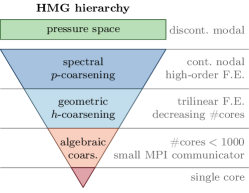
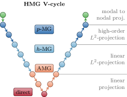
Figure 4: Hybrid spectral-geometric-algebraic multigrid (HMG). Left: Illustration of multigrid hierarchy. From top to bottom, first, the multigrid levels are obtained by spectral coarsening (dark blue). Next, the mesh is geometrically coarsened and repartitioned on successively fewer cores to minimize communication (light blue). Finally, AMG further reduces problem size and core count (light red). The multigrid hierarchy for the pressure Poisson operator $\mathbf{K}_{w_{r}}$ additionally involves smoothing in the discontinuous, modal pressure space (green). The projection from the discontinuous, modal to a continuous finite element nodal basis uses a lumped mass matrix in the nodal space to avoid the global mass matrix system solve. Right: The multigrid V-cycle consists of smoothing at each level of the hierarchy (circles) and intergrid transfer operators (arrows downward for restriction and arrows upward for interpolation). To enhance efficacy of the the V-cycle as a preconditioner, different types of projection operators are employed for these operators depending on the phase within the V-cycle.

7 Algorithmic and parallel scalability for $\text{HMG}\!+\!\text{w-BFBT}$ Stokes preconditioner

After establishing the robustness of the Stokes solver with w-BFBT preconditioning in theory (Section 3) and numerically (Section 4), addressing issues associated with Dirichlet boundary conditions (Section 5), and introducing an effective and scalable multigrid method (Section 6), in this section we finally study the scalability of the Stokes solver building on $\text{HMG}\!+\!\text{w-BFBT}$. One aspect of scalability is algorithmic scalability, i.e., the dependence of Krylov iterations on the mesh resolution and the discretization order. The second aspect is parallel scalability of the implementation, i.e., runtime measured on increasing numbers of compute cores. Studying both aspects is required to fully assess the performance of a solver at scale.

The algorithmic scalability in Table 3 shows results for the Stokes solver as well as its individual components by reporting iteration numbers for solving the systems $\mathbf{A}\mathbf{u}=\mathbf{f}$ and $\mathbf{K}_{w_{r}}\mathbf{p}=\mathbf{g}$. Studying the individual components allows us to observe HMG performance in isolation and to compare it to the algorithmic scalability of the full Stokes system, which is indicative of the quality of the w-BFBT Schur complement approximation. All systems are solved with preconditioned GMRES down to a relative tolerance of $10^{-6}$. The preconditioners for $\mathbf{A}$ and $\mathbf{K}_{w_{r}}$ are HMG-V-cycles as described in Section 6. For the w-BFBT preconditioner, we set a constant left boundary amplification $a_{l}=1$ and vary the right boundary amplification $a_{r}$ according to results from Section 5. The iteration counts in Table 3(a) show textbook mesh independence when increasing the level of refinement $\ell$. This holds for each component, $\mathbf{A}$ and $\mathbf{K}_{w_{r}}$, and also the whole Stokes solver, and hence we conclude that the Schur complement approximation by w-BFBT is mesh-independent. When the discretization order $k$ is increased, the iteration counts presented in Table 3(b) increase mildly. The convergence of both components $\mathbf{A}$ and $\mathbf{K}_{w_{r}}$ exhibits a moderate dependence on $k$. Since the increase in number of iterations is sightly larger for the full Stokes solve than for $\mathbf{A}$ and $\mathbf{K}_{w_{r}}$, we suspect a mild deterioration of w-BFBT as a Schur complement approximation.

Table 3: Algorithmic scalability for Stokes solver with $\text{HMG}\!+\!\text{w-BFBT}$ preconditioning while 3(a) varying mesh refinement level $\ell$ and 3(b) varying discretization order $k$ (problem S16-rand, $\operatorname{DR}(\mu)=10^{6}$). Computational cost is expressed in number of GMRES iterations (abbreviated by It.) for full Stokes solve ($10^{-6}$ residual reduction). Left boundary amplification for $\mathbf{C}_{w_{l}}$ is fixed to $a_{l}=1$; right boundary amplification $a_{r}$ for $\mathbf{D}_{w_{r}}$ varies. Additionally, the numbers of GMRES iterations for solving only the sub-systems $\mathbf{A}\mathbf{u}=\mathbf{f}$ and $\mathbf{K}_{w_{r}}\mathbf{p}=\mathbf{g}$ are given for demonstration of HMG efficacy (here, $\mathbf{f}$ is the right-hand side of the momentum equation and $\mathbf{g}$ is the discreet representation of $\nabla\cdot\boldsymbol{f}$; however, random right-hand sides would give similar convergence results).

(a) Algorithmic scalability (fixed order $k=2$)

$\ell$	$a_{r}$	$\boldsymbol{u}$-DOF	It.	$p$-DOF	It.	DOF	It.
		$[\times 10^{6}]$	$\mathbf{A}$	$[\times 10^{6}]$	$\mathbf{K}_{w_{r}}$	$[\times 10^{6}]$	Stokes
4	1	0.11	18	0.02	8	0.12	40
5	2	0.82	18	0.13	7	0.95	33
6	4	6.44	18	1.05	6	7.49	33
7	8	50.92	18	8.39	6	59.31	34
8	16	405.02	18	67.11	6	472.12	34
9	32	3230.67	18	536.87	6	3767.54	34
10	64	25807.57	18	4294.97	6	30102.53	34

(b) Algorithmic scalability (fixed level $\ell=5$)

$k$	$a_{r}$	$\boldsymbol{u}$-DOF	It.	$p$-DOF	It.	DOF	It.
		$[\times 10^{6}]$	$\mathbf{A}$	$[\times 10^{6}]$	$\mathbf{K}_{w_{r}}$	$[\times 10^{6}]$	Stokes
2	2	0.82	18	0.13	7	0.95	33
3	4	2.74	20	0.32	8	3.07	37
4	8	6.44	20	0.66	7	7.10	36
5	16	12.52	23	1.15	12	13.67	43
6	32	21.56	23	1.84	12	23.40	50
7	64	34.17	22	2.75	10	36.92	54
8	128	50.92	22	3.93	10	54.86	67

The following parallel scalability results complement the results presented in [36], where scalability to millions of threads was demonstrated on IBM’s BlueGene/Q architecture, which is specifically designed for large-scale supercomputers and thus differs from conventional clusters. The parallel scalability results here were obtained on the full Lonestar 5 peta-scale system, which represents a rather conventional cluster, housed at the Texas Advanced Computing Center (TACC). The Lonestar 5 supercomputer entered production in January 2016 and is a Cray XC40 system consisting of 1252 compute nodes. Each node is equipped with two Intel Haswell 12-core processors (Xeon E5-2680v3) and 64 GBytes of memory. Inter-node communication is based on an Aries Dragonfly topology network that provides dynamic routing and thus enables optimal use of the system bandwidth.

Results for weak scalability (DOF/core fixed to $\sim$1 million) in Figure 5(a) show that the Stokes solver with w-BFBT (blue curve) maintains 90% parallel efficiency over a 618-fold increase in degrees of freedom along with cores. Even for the setup of the Stokes solver (green curve), which mainly involves generation of the HMG hierarchy, we observe 71% parallel efficiency. These are excellent results for such a complex implicit multilevel solver with optimal algorithmic performance (when the mesh is refined, or nearly algorithmically optimal when the order is increased) and with convergence that is independent of the number of cores.

Finally, Figure 5(b) reports strong scalability results (overall DOF fixed to 59 million) and how the number of OpenMP threads substituting MPI ranks influences speedup. Over the 78-fold increase from 48 to 3744 cores, efficiency reduces moderately, to a worst-case 68% for 24$\times$OMP1. However, note that in the largest run with 29,640 cores, the granularity is only $\sim$2000 DOF/core, which is extremely challenging for strong scalability. In this case, due to the increased communication volume, overlapping with decreased amounts of computation becomes impossible and communication dominates the runtime. This behavior is expected for an implicit solver, especially for a multilevel method that does not sacrifice algorithmic optimality for parallel scalability.

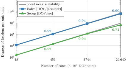
(a) Weak scalability ($k=2$, $\ell=7,\ldots,10$)

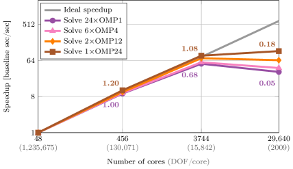
(b) Strong scalability ($k=2$, $\ell=7$)

Figure 5: Parallel scalability on Lonestar 5 for Stokes solver with $\text{HMG}\!+\!\text{w-BFBT}$ preconditioning (problem S16-rand, $\operatorname{DR}(\mu)=10^{6}$ as in Table 3(a)). 5(a) Weak scalability of setup and solve phases (normalized w.r.t. deviations from const. DOF/core). Numbers along the graph lines indicate weak parallel efficiency w.r.t. ideal weak scalability (baseline is 48 cores result). DOF/core is $\sim$1 million; the largest problem size on 29,640 cores has 30 billion DOF. 5(b) Strong scalability of solve phase for different configurations of OpenMP threads (OMP) substituting MPI ranks on each node consisting of 24 cores. Numbers along the graph lines indicate strong efficiency w.r.t. ideal speedup (baseline is 48 cores result).

8 Conclusions

For Stokes flow problems with highly heterogeneous viscosity, the commonly used inverse viscosity-weighted mass matrix approximation of the Schur complement can be insufficient. As a consequence, convergence of Schur complement-based Krylov solvers can be extremely slow. While each iteration with the weighted BFBT (w-BFBT) Schur complement approximation proposed in this paper is computationally more costly, we observe that it results in robust and fast convergence even for complex viscosity structures and for up to ten orders of magnitude viscosity contrasts—properties than occur, for instance, in problems involving non-Newtonian geophysical fluids. Our numerical findings are supported by theoretical spectral equivalence results. To the best of our knowledge, a similar analysis has not been shown for any BFBT-type method before.

At Dirichlet boundaries, we use a modification of w-BFBT that is necessary for mesh-independent convergence. In this modification, we dampen the influence of elements at these boundaries, which would otherwise dominate in w-BFBT and degrade its efficacy as a preconditioner. Finding an alternative remedy is a subject of current research.

Indefinite problems with highly heterogeneous coefficients and high-order discretizations present significant challenges for efficient solvers, especially in parallel. Nevertheless, we have demonstrated that with careful attention paid to algorithm design and scalable implementation, viscosity-robust and mesh-independent solvers can be designed that exhibit nearly optimal algorithmic and parallel scalability over a wide range of problems sizes and core counts.

References

- [1] Gabriel Acosta, Ricardo G. Durán, and Ariel L. Lombardi, Weighted Poincaré and Korn inequalities for Hölder domains, Mathematical Methods in the Applied Sciences, 29 (2006), pp. 387–400.
- [2] Satish Balay, Shrirang Abhyankar, Mark F. Adams, Jed Brown, Peter Brune, Kris Buschelman, Lisandro Dalcin, Victor Eijkhout, William D. Gropp, Dinesh Kaushik, Matthew G. Knepley, Lois Curfman McInnes, Karl Rupp, Barry F. Smith, Stefano Zampini, and Hong Zhang, PETSc users manual, Tech. Report ANL-95/11 - Revision 3.6, Argonne National Laboratory, 2015.
- [3] Wolfgang Bangerth and Timo Heister, ASPECT: Advanced Solver for Problems in Earth’s ConvecTion, Computational Infrastructure in Geodynamics, 2015.
- [4] Michele Benzi, Gene H. Golub, and Jörg Liesen, Numerical solution of saddle point problems, Acta Numerica, 14 (2005), pp. 1–137.
- [5] Carsten Burstedde, Omar Ghattas, Michael Gurnis, Tobin Isaac, Georg Stadler, Tim Warburton, and Lucas C. Wilcox, Extreme-scale AMR, in SC10: Proceedings of the International Conference for High Performance Computing, Networking, Storage and Analysis, ACM/IEEE, 2010.
- [6] Carsten Burstedde, Omar Ghattas, Michael Gurnis, Eh Tan, Tiankai Tu, Georg Stadler, Lucas C. Wilcox, and Shijie Zhong, Scalable adaptive mantle convection simulation on petascale supercomputers, in SC08: Proceedings of the International Conference for High Performance Computing, Networking, Storage and Analysis, ACM/IEEE, 2008.
- [7] Carsten Burstedde, Omar Ghattas, Georg Stadler, Tiankai Tu, and Lucas C. Wilcox, Parallel scalable adjoint-based adaptive solution for variable-viscosity Stokes flows, Computer Methods in Applied Mechanics and Engineering, 198 (2009), pp. 1691–1700.
- [8] Carsten Burstedde, Georg Stadler, Laura Alisic, Lucas C. Wilcox, Eh Tan, Michael Gurnis, and Omar Ghattas, Large-scale adaptive mantle convection simulation, Geophysical Journal International, 192 (2013), pp. 889–906.
- [9] Carsten Burstedde, Lucas C. Wilcox, and Omar Ghattas, p4est: Scalable algorithms for parallel adaptive mesh refinement on forests of octrees, SIAM Journal on Scientific Computing, 33 (2011), pp. 1103–1133.
- [10] Seng-Kee Chua and Richard L. Wheeden, Estimates of best constants for weighted Poincaré inequalities on convex domains, Proceedings of the London Mathematical Society, 93 (2006), pp. 197–226.
- [11] Michel Crouzeix and Pierre-Arnaud Raviart, Conforming and nonconforming finite element methods for solving the stationary Stokes equations. I, Rev. Française Automat. Informat. Recherche Opérationnelle Sér. Rouge, 7 (1973), pp. 33–75.
- [12] Jean Donea and Antonio Huerta, Finite Element Methods for Flow Problems, John Wiley & Sons, 2003.
- [13] Howard C. Elman, Preconditioning for the steady-state Navier–Stokes equations with low viscosity, SIAM Journal on Scientific Computing, 20 (1999), pp. 1299–1316.
- [14] Howard C. Elman, Victoria E. Howle, John Shadid, Robert Shuttleworth, and Raymond S. Tuminaro, Block preconditioners based on approximate commutators, SIAM Journal on Scientific Computing, 27 (2006), pp. 1651–1668.
- [15] , A taxonomy and comparison of parallel block multi-level preconditioners for the incompressible Navier–Stokes equations, Journal of Computational Physics, 227 (2008), pp. 1790–1808.
- [16] Howard C. Elman, David J. Silvester, and Andrew J. Wathen, Finite elements and fast iterative solvers: with applications in incompressible fluid dynamics, Oxford University Press, 2014.
- [17] Howard C. Elman and Raymond S. Tuminaro, Boundary conditions in approximate commutator preconditioners for the Navier–Stokes equations, Electronic Transactions on Numerical Analysis, 35 (2009), pp. 257–280.
- [18] Mikito Furuichi, Dave A. May, and Paul J. Tackley, Development of a Stokes flow solver robust to large viscosity jumps using a Schur complement approach with mixed precision arithmetic, Journal of Computational Physics, 230 (2011), pp. 8835–8851.
- [19] Roland Glowinski and Jinchao Xu, Numerical Methods for Non-Newtonian Fluids: Special Volume, vol. 16 of Handbook of Numerical Analysis, North-Holland, 2011.
- [20] Piotr P. Grinevich and Maxim A. Olshanskii, An iterative method for the Stokes-type problem with variable viscosity, SIAM Journal on Scientific Computing, 31 (2009), pp. 3959–3978.
- [21] Vincent Heuveline and Friedhelm Schieweck, On the inf-sup condition for higher order mixed FEM on meshes with hanging nodes, ESAIM: Mathematical Modelling and Numerical Analysis, 41 (2007), pp. 1–20.
- [22] Kolumban Hutter, Theoretical Glaciology, Mathematical Approaches to Geophysics, D. Reidel Publishing Company, 1983.
- [23] Tobin Isaac, Noemi Petra, Georg Stadler, and Omar Ghattas, Scalable and efficient algorithms for the propagation of uncertainty from data through inference to prediction for large-scale problems, with application to flow of the Antarctic ice sheet, Journal of Computational Physics, 296 (2015), pp. 348–368.
- [24] Tobin Isaac, Georg Stadler, and Omar Ghattas, Solution of nonlinear Stokes equations discretized by high-order finite elements on nonconforming and anisotropic meshes, with application to ice sheet dynamics, SIAM Journal on Scientific Computing, 37 (2015), pp. B804–B833.
- [25] Volker John, Kristine Kaiser, and Julia Novo, Finite element methods for the incompressible Stokes equations with variable viscosity, ZAMM - Zeitschrift für Angewandte Mathematik und Mechanik, 96 (2016), pp. 205–216.
- [26] David Kay, Daniel Loghin, and Andrew Wathen, A preconditioner for the steady-state Navier-Stokes equations, SIAM Journal on Scientific Computing, 24 (2002), pp. 237–256.
- [27] Martin Kronbichler, Timo Heister, and Wolfgang Bangerth, High accuracy mantle convection simulation through modern numerical methods, Geophysical Journal International, 191 (2012), pp. 12–29.
- [28] Anders Logg, Kent-Andre Mardal, and Garth Wells, Automated Solution of Differential Equations by the Finite Element Method: The FEniCS book, vol. 84, Springer Science & Business Media, 2012.
- [29] Dave A. May, Jed Brown, and Laetitia Le Pourhiet, pTatin3D: High-performance methods for long-term lithospheric dynamics, in SC14: Proceedings of the International Conference on High Performance Computing, Networking, Storage and Analysis, IEEE Press, 2014, pp. 274–284.
- [30] Dave A. May, Jed Brown, and Laetitia Le Pourhiet, A scalable, matrix-free multigrid preconditioner for finite element discretizations of heterogeneous Stokes flow, Computer Methods in Applied Mechanics and Engineering, 290 (2015), pp. 496–523.
- [31] Dave A. May and Louis Moresi, Preconditioned iterative methods for Stokes flow problems arising in computational geodynamics, Physics of the Earth and Planetary Interiors, 171 (2008), pp. 33–47.
- [32] Dan McKenzie, The generation and compaction of partially molten rock, Journal of Petrology, 25 (1984), pp. 713–765.
- [33] Clemens Pechstein and Robert Scheichl, Weighted Poincaré inequalities, IMA Journal of Numerical Analysis, 33 (2013), pp. 652–686.
- [34] Noemi Petra, Hongyu Zhu, Georg Stadler, Thomas J. R. Hughes, and Omar Ghattas, An inexact Gauss-Newton method for inversion of basal sliding and rheology parameters in a nonlinear Stokes ice sheet model, Journal of Glaciology, 58 (2012), pp. 889–903.
- [35] Kumbakonam R. Rajagopal, Mechanics of non-Newtonian fluids, in Recent Developments in Theoretical Fluid Mechanics, G.P. Galdi and J. Necas, eds., vol. 291, Longman’s Scientific and Technical, 1993, pp. 129–162.
- [36] Johann Rudi, A. Crisiano I. Malossi, Tobin Isaac, Georg Stadler, Michael Gurnis, Yves Ineichen, Costas Bekas, Alessandro Curioni, and Omar Ghattas, An extreme-scale implicit solver for complex PDEs: Highly heterogeneous flow in earth’s mantle, in SC15: Proceedings of the International Conference for High Performance Computing, Networking, Storage and Analysis, ACM, 2015, pp. 5:1–5:12.
- [37] Gerald Schubert, Donald L. Turcotte, and Peter Olson, Mantle Convection in the Earth and Planets, Cambridge University Press, 2001.
- [38] David J. Silvester, Howard C. Elman, David Kay, and Andrew J. Wathen, Efficient preconditioning of the linearized Navier–Stokes equations for incompressible flow, Journal of Computational and Applied Mathematics, 128 (2001), pp. 261–279. Numerical analysis 2000, Vol. VII, Partial differential equations.
- [39] Georg Stadler, Michael Gurnis, Carsten Burstedde, Lucas C. Wilcox, Laura Alisic, and Omar Ghattas, The dynamics of plate tectonics and mantle flow: From local to global scales, Science, 329 (2010), pp. 1033–1038.
- [40] Rolf Stenberg and Manil Suri, Mixed finite element methods for problems in elasticity and Stokes flow, Numerische Mathematik, 72 (1996), pp. 367–389.
- [41] Hari Sundar, George Biros, Carsten Burstedde, Johann Rudi, Omar Ghattas, and Georg Stadler, Parallel geometric-algebraic multigrid on unstructured forests of octrees, in SC12: Proceedings of the International Conference for High Performance Computing, Networking, Storage and Analysis, Salt Lake City, UT, 2012, ACM/IEEE.
- [42] Rüdiger Verfürth, A Posteriori Error Estimation Techniques for Finite Element Methods, Oxford University Press, 2013.
- [43] Jennifer Worthen, Georg Stadler, Noemi Petra, Michael Gurnis, and Omar Ghattas, Towards adjoint-based inversion for rheological parameters in nonlinear viscous mante flow, Physics of the Earth and Planetary Interiors, 234 (2014), pp. 23–34.