Shear viscosity at the Ising-nematic quantum critical point
in two dimensional metals

Abstract

In an isotropic strongly interacting quantum liquid without quasiparticles, general scaling arguments imply that the dimensionless ratio $(k_{B}/\hbar)\,\eta/s$, where $\eta$ is the shear viscosity and $s$ is the entropy density, is a universal number. We compute the shear viscosity of the Ising-nematic critical point of metals in spatial dimension $d=2$ by an expansion below $d=5/2$. The anisotropy associated with directions parallel and normal to the Fermi surface leads to a violation of the scaling expectations: $\eta$ scales in the same manner as a chiral conductivity, and the ratio $\eta/s$ diverges at low temperature ($T$) as $T^{-2/z}$, where $z$ is the dynamic critical exponent for fermionic excitations dispersing normal to the Fermi surface.

I Introduction

Recent experiments on graphene Bandurin et al. (2016); Crossno et al. (2016) and PdCoO₂ Moll et al. (2016) have displayed remarkable evidence for nearly-momentum-conserving hydrodynamic flow of the electron liquid. In clean Fermi liquids, hydrodynamic flow requires very clean samples with weak umklapp scattering so that electron-electron collisions lead to thermalization before there is significant momentum lost to the crystal Moll et al. (2016); Gurzhi (1968); de Jong and Molenkamp (1995); Andreev et al. (2011). However, rapid thermalization and hydrodynamics are natural properties of quantum critical systems Damle and Sachdev (1997) and strange metals Hartnoll et al. (2007, 2014); Patel and Sachdev (2014); Lucas and Sachdev (2015), and their consequences should be visible even in moderately clean samples. Graphene was proposed as a strange metal in which ill-defined quasiparticles lead to hydrodynamic flow at intermediate temperatures Müller and Sachdev (2008); Fritz et al. (2008); Müller et al. (2008); Foster and Aleiner (2009); Müller et al. (2009); Mendoza et al. (2011); Tomadin et al. (2014); Principi and Vignale (2015); Torre et al. (2015); Levitov and Falkovich (2016); Lucas et al. (2016); Falkovich and Levitov (2016): the experiments also display evidence Torre et al. (2015); Levitov and Falkovich (2016); Lucas et al. (2016); Bandurin et al. (2016); Crossno et al. (2016) for the viscous drag of such flow. There have also been studies of viscous flow in high energy physics Policastro et al. (2001); Kovtun et al. (2005); Karsch et al. (2008); Heinz et al. (2012) and ultracold atoms Cao et al. (2011); Taylor and Randeria (2010); Enss et al. (2011); Kryjevski (2014); Bluhm and Schäfer (2016).

These experimental advances indicate that the time is ripe for exploring hydrodynamic electron flow in the ubiquitous strange metal regimes of the cuprates or the pnictides. These are metals without quasiparticle excitations, and so should exhibit hydrodynamic flow when impurities are dilute. We note the indirect evidence for such behavior in the photoemission experiments of Rameau et al. Rameau et al. (2014). To this end, here we examine the simplest model which realizes a metallic state without quasiparticles in two spatial dimensions, and compute its shear viscosity, $\eta$. We will study the quantum critical point (QCP) for the onset of Ising nematic order Halboth and Metzner (2000); Oganesyan et al. (2001); Metzner et al. (2003) using its continuum field theoretic formulation using patches on the Fermi surface Metlitski and Sachdev (2010); Dalidovich and Lee (2013).

General scaling arguments (reviewed below) for a spatially isotropic system imply that $\eta$ should scale in the same manner as the entropy density, $s$; so

$$\eta/s\sim\hbar/k_{B},$$ (1)

where the r.h.s. restores dimensions, and the prefactor is expected to be of order unity. (In $d=2$ hydrodynamic long time tails can lead to logarithmic corrections to $\eta$ Kovtun (2012) which we ignore here, as we find much larger corrections). This is also the expectation from holographic studies of critical quantum liquids Policastro et al. (2001); Kovtun et al. (2005); Iqbal and Liu (2009); Roychowdhury (2015); Kiritsis and Matsuo (2015); Kuang and Wu (2015); Kolekar et al. (2016). A relationship of the form (1) appeared in string-theoretic realizations of strongly-coupled field theories Kovtun et al. (2005), and has been widely used as a diagnostic of strongly-coupled non-quasiparticle dynamics in the quark-gluon plasma Policastro et al. (2001); Kovtun et al. (2005); Karsch et al. (2008); Heinz et al. (2012).

Our main result is that Eq. (1) does not apply to many of the models of electronic strange metals without quasiparticles. Even without long-lived quasiparticles, such models have a Fermi surface at $T=0$, which defines momenta with singular low energy excitations; more precisely, the Fermi surface is the locus of points at which the inverse Green’s function vanishes. Although the metal is globally isotropic, the excitations in the vicinity of a particular point on the Fermi surface have a highly anisotropic structure, as shown in Fig. 1: excitations at a momentum $k_{\perp}$ perpendicular to the Fermi surface have a typical energy $k_{\perp}^{z}$, while excitations at a momentum $k_{\parallel}$ parallel to the Fermi surface have a typical energy $k_{\parallel}^{2z}$; here $z$ is the dynamic critical exponent.

Figure 1: Fermi surface and definition of the momentum components parallel ($k_{\parallel}$) and perpendicular ($k_{\perp}$) to the Fermi surface at the two Fermi surface patches in which the low-energy field theory is defined.

In the present paper, we will show that the dispersion of the excitations parallel to the Fermi surface plays a more fundamental role in determining the value of the shear viscosity $\eta$. As a result Eq. (1) does not apply, and we find instead a divergence as $T\rightarrow 0$,

$$\eta/s\sim T^{-2/z}.$$ (2)

This surprising violation of (1) in an isotropic system can be traced directly to the presence of a Fermi surface. Our result implies that holographic duals of strange metals Liu et al. (2011); Čubrović et al. (2009); Charmousis et al. (2010); Goldstein et al. (2010); Ogawa et al. (2012); Huijse et al. (2012) do not fully capture the Fermi surface structure. Instead, it appears that bulk quantum gravity corrections will be required to resurrect the Fermi surface in the holographic theories Polchinski and Silverstein (2012); Faulkner and Iqbal (2013); Sachdev (2012), and to obtain the result corresponding to Eq. (2).

Section II will present a review of scaling arguments which usually apply the conventional relation in Eq. (1). The dimensionally extended field theory for the quantum critical point will be presented in Section III. We will use this field theory to compute the ‘optical’ shear viscosity (i.e. the viscosity at frequencies $\omega\gg T$) in Section IV. We will then examine the usual DC viscosity (at frequencies $\omega\ll T$) in Section V.

II Scaling arguments

In studies so far of the thermodynamic and transport properties of strange metals, the anisotropy of the Fermi surface has had a specific consequence Eberlein et al. (2016): the entropy density, and the electrical and thermal conductivities are dominated by the energy dispersion perpendicular to the Fermi surface, while the direction parallel to the Fermi surface mostly acts as a label which counts the total density of perpendicular excitations. Consequently, in scaling arguments we find a violation of hyperscaling: this is the property in which the entropy density of a $d$ dimensional system scales as if it is in $d-\theta$ dimensions, with $\theta$ the violation of hyperscaling exponent. For a Fermi surface $\theta=d-1$, because only the dispersion perpendicular to each point on the Fermi surface is important in the computation of the entropy. Recent work has shown Eberlein et al. (2016) that similar arguments also correctly determine the electrical conductivity and entropy density.

We now review the general scaling arguments for the universality of $\eta/s$. The entropy density invariably scales as a density, and so has scaling dimension $d$. From the arguments just presented above, with the violation of hyperscaling in the presence of a Fermi surface, the entropy density $s$ should have scaling dimension $d-\theta$, and so

$$s\sim T^{(d-\theta)/z};$$ (3)

this was confirmed by computations in Eberlein et al. (2016). Similar arguments apply to the optical conductivity $\sigma_{Q}(\omega)$, where $\omega$ is a frequency; naively, the conductivity has scaling dimension $d-2$, and so we can expect that in the presence of a Fermi surface, the dimension will be $d-\theta-2$. The computation in Eberlein et al. (2016) shows that this is indeed the case, and we have

$$\sigma_{Q}\sim T^{(d-2-\theta)/z}\Upsilon(\omega/T),$$ (4)

where $\Upsilon$ is a scaling function.

In an isotropic system that obeys hyperscaling, we can read off the scaling dimension of the stress tensor from its definition Schwartz (2014),

$$T_{\mu\nu}=\sum_{n}\Bigl{(}\frac{\delta\mathcal{L}}{\delta(\partial_{\mu}\zeta_{n})}\partial_{\nu}\zeta_{n}-\partial_{\mu}\frac{\delta\mathcal{L}}{\delta(\partial^{2}_{\mu}\zeta_{n})}\partial_{\nu}\zeta_{n}\Bigr{)}-\delta_{\mu\nu}\mathcal{L},$$ (5)

where $\zeta_{n}$ denotes all the fields in the theory and $\mathcal{L}$ the Lagrangian density. It follows that the spatial components have the same scaling dimension as the Lagrangian density, $[T_{ij}]=d+z$, and that the mixed temporal-spatial components have scaling dimension $[T_{0i}]=d+1$. Inserting these scaling dimensions into the Euler equation,

$$\partial_{t}p_{\alpha}=\partial_{\beta}T_{\alpha\beta},$$ (6)

where $p_{\alpha}$ are the components of the momentum operator, yields consistent results. We thus obtain

$$[T_{xy}]=d+z$$ (7)

in the presence of hyperscaling. Kubo’s formula for the frequency-dependent shear viscosity reads Taylor and Randeria (2010); Enss et al. (2011),

$$\operatorname{Re}\eta(\omega)=\lim_{\bm{q}\rightarrow 0}\omega^{-1}\operatorname{Im}\chi_{T_{xy}T_{xy}}(\omega,\bm{q}),$$ (8)

where

$$\chi_{T_{xy}T_{xy}}(i\omega_{n},\bm{q})=\langle T_{xy}(i\omega_{n},\bm{q})T_{xy}(-i\omega_{n},-\bm{q})\rangle$$ (9)

is the autocorrelation function of the $xy$-component of the stress tensor $T$. Its scaling dimension is

$$[\eta]=-z-d-z+2[T_{xy}]=d$$ (10)

and the d.c. shear viscosity is given by $\eta=\lim_{\omega\rightarrow 0}\eta(\omega)$. This is the same scaling dimension as for the entropy density above. With the violation of hyperscaling in the presence of a Fermi surface, the examples of the entropy density and the optical conductivity above suggest that $\eta$ should scale just like $s$ in Eq. (3), and hence Eq. (1) should apply. Our computations in this paper show that this is not true, and the Fermi surface leads to behavior genuinely different both from naive scaling assumptions, and from holographic examples: the $T$ dependence of $\eta$ is such that Eq. (2) holds.

III Field theory

We now recall the field theory which allow us to formulate a systematic and controlled renormalization group analysis using a convenient dimensional regularization method. Moreover, this method fully preserves a two-dimensional Fermi surface with anisotropic dispersion in the vicinity of every point on the Fermi surface, and these features are crucial for our results. We will discuss the field theory for the Ising-nematic critical point, but similar field theories and results also apply to the problem of a Fermi surface coupled to a gauge field, or to other long-wavelength order parameters Metlitski and Sachdev (2010).

We consider a theory of fermions, $\psi$, in $(2+1)$ dimensions which are coupled to a critical boson, $\Phi$,

$$\begin{split}S(\bar{\psi},\psi,\Phi)=&\sum_{s=\pm}\sum_{j=1}^{N}\int\frac{d^{3}k}{(2\pi)^{3}}\tilde{\psi}^{\dagger}_{sj}(k)(ik_{0}+sk_{x}+k_{y}^{2})\tilde{\psi}_{sj}(k)+\frac{1}{2}\int\frac{d^{3}k}{(2\pi)^{3}}(k_{0}^{2}+k_{x}^{2}+k_{y}^{2})\Phi(-k)\Phi(k)\\ &+\frac{e}{\sqrt{N}}\sum_{s=\pm}\sum_{j=1}^{N}\int\frac{d^{3}k}{(2\pi)^{3}}\int\frac{d^{3}q}{(2\pi)^{3}}\lambda_{s}\Phi(q)\tilde{\psi}^{\dagger}_{sj}(k+q)\tilde{\psi}_{sj}(k),\end{split}$$ (11)

where $e$ is the fermion-boson coupling constant, $s=\pm 1$ labels the two Fermi surface patches, $N$ is the number of fermionic flavors and $\lambda_{s}$ equals 1 ($s$) for the Ising-nematic critical point (fermions coupled to a $U(1)$ gauge field). This model has been studied by many authors, including Refs. Metlitski and Sachdev, 2010; Dalidovich and Lee, 2013. In the following, we restrict ourselves to the Ising-nematic critical point and set $\lambda_{s}=1$.

This model can be studied in a controlled way using the dimensional regularization scheme proposed by Dalidovich and Lee Dalidovich and Lee (2013). Increasing the codimension of the Fermi surface by introducing auxiliary time-like directions, the dimensionally regularized action in $(d+1)$ dimensions reads

$$\begin{split}S(\bar{\psi},\psi,\Phi)=&\sum_{j=1}^{N}\int\frac{d^{d+1}k}{(2\pi)^{d+1}}\bar{\psi}_{j}(k)[i\bm{\Gamma}\cdot\bm{K}+i\gamma_{x}\delta_{k}]\psi_{j}(k)+\frac{1}{2}\int\frac{d^{d+1}q}{(2\pi)^{d+1}}[\bm{Q}^{2}+q_{x}^{2}+q_{y}^{2}]\Phi(-q)\Phi(q)\\ &+\frac{ie}{\sqrt{N}}\sqrt{d-1}\sum_{j=1}^{N}\int\frac{d^{d+1}k}{(2\pi)^{d+1}}\int\frac{d^{d+1}q}{(2\pi)^{d+1}}\Phi(q)\bar{\psi}_{j}(k+q)\gamma_{x}\psi_{j}(k),\end{split}$$ (12)

where $\bm{K}=(k_{0},k_{1},\ldots,k_{d-2})$ collects the physical and $(d-2)$ auxiliary frequency variables. We introduced the spinor notation

$$\psi_{j}(k) =\begin{pmatrix}\tilde{\psi}_{+,j}(k),\tilde{\psi}^{\dagger}_{-,j}(-k)\end{pmatrix}^{T} \bar{\psi}_{j}(k) =\psi^{\dagger}_{j}(k)\gamma_{0}$$ (13)

and defined the gamma matrices as $\gamma_{0}=\sigma_{y}$ and $\gamma_{x}=\sigma_{x}$ for the spatial and as $\bm{\Gamma}=(\gamma_{0},\gamma_{1},\ldots,\gamma_{d-2})$ for the time-like directions. Within a patch, we choose $k_{x}$ ($k_{y}$) perpendicular (parallel) to the Fermi surface, as shown in Fig. 1. The dispersion in the spatial plane containing the Fermi surface is $\delta_{k}$, while the full dispersion is $\varepsilon_{k}$ with

$$\delta_{k}=k_{x}+\sqrt{d-1}k_{y}^{2}\quad,\quad\varepsilon_{k}=\left(\delta_{k}^{2}+\sum_{i=1}^{d-2}k_{i}^{2}\right)^{1/2}.$$ (14)

Note the line of zero energy excitations in the plane $k_{i}=0$ which represents a patch on the Fermi surface in Fig. 1, and the relativistic dispersion along the $k_{i}$ directions.

Rescaling momenta as

$$\bm{K} =b^{-1}\bm{K}^{\prime} k_{x} =b^{-1}k_{x}^{\prime} k_{y}=b^{-1/2}k_{y}^{\prime},$$ (15)

the fermionic quadratic part of the action and the contribution $\sim q_{y}^{2}$ in the bosonic quadratic part of the action are invariant under rescaling if fields are scaled as

$$\psi_{j}(k) =b^{d/2+3/4}\psi_{j}^{\prime}(k^{\prime}) \Phi(k) =b^{d/2+3/4}\Phi^{\prime}(k^{\prime})$$ (16)

The terms proportional to $\bm{Q}^{2}$ and $q_{x}^{2}$ in the bosonic quadratic part are irrelevant under this rescaling. The coupling scales as

$$e^{\prime}=eb^{\frac{1}{2}(5/2-d)},$$ (17)

identifying $d=5/2$ as the upper critical dimension. It is irrelevant for $d>5/2$ and relevant for $d<5/2$. This allows to access non-Fermi liquid physics perturbatively by using $\epsilon=5/2-d$ as expansion parameter.

Keeping only marginal terms, the ansatz for the local field theory reads

$$\begin{split}S(\bar{\psi},\psi,\Phi)=&\sum_{j=1}^{N}\int\frac{d^{d+1}k}{(2\pi)^{d+1}}\bar{\psi}_{j}(k)[i\bm{\Gamma}\cdot\bm{K}+i\gamma_{x}\delta_{k}]\psi_{j}(k)+\frac{1}{2}\int\frac{d^{d+1}q}{(2\pi)^{d+1}}q_{y}^{2}\Phi(-q)\Phi(q)\\ &+\frac{ie\mu^{\epsilon/2}}{\sqrt{N}}\sqrt{d-1}\sum_{j=1}^{N}\int\frac{d^{d+1}k}{(2\pi)^{d+1}}\int\frac{d^{d+1}q}{(2\pi)^{d+1}}\Phi(q)\bar{\psi}_{j}(k+q)\gamma_{x}\psi_{j}(k),\end{split}$$ (18)

where we introduced the momentum scale $\mu$ in order to make the coupling $e$ dimensionless. Perturbative corrections to this action at one-loop level reintroduce dynamics for the bosonic field. The $\epsilon=5/2-d$ expansion allows us to make a renormalized perturbative computation in the dimensionless coupling $e$. Note that this is not equivalent to a simple $1/N$ expansion, which breaks down at the Ising-nematic QCP Metlitski and Sachdev (2010), and that the expansion parameter is $\frac{e^{4/3}}{N}$ Dalidovich and Lee (2013).

IV Optical shear viscosity

In the following, we focus on the ‘optical’ shear viscosity, evaluated at frequencies $\omega\gg T$. Its evaluation is simpler than that for the d.c. viscosity, $\omega\ll T$, which will be considered in Section V.

For the Ising-nematic QCP the $xy$-component of the stress tensor is proportional to the $y$-component of the ‘chiral’ current operator,

$$\begin{split}T_{xy}(q)&=i\sum_{j=1}^{N}\int_{k}\bigl{(}k_{y}+\frac{q_{y}}{2}\bigr{)}\bar{\psi}_{j}(k+q)\gamma_{x}\psi_{j}(k)\\ &=\frac{1}{2\sqrt{d-1}}J_{y}(q).\end{split}$$ (19)

where $\int_{k}=\int\frac{dk_{x}}{2\pi}{}\int\frac{dk_{y}}{2\pi}{}\int\frac{d^{d-1}K}{(2\pi)^{d-1}}$. Note that the $x$- and $y$-components of the chiral current contain the same gamma matrix.

Figure 2: Feynman diagrams yielding the renormalization of the scaling behavior of the viscosity at lowest order in $\epsilon$: (a) One-loop contribution, (b) self-energy correction and (c) vertex correction. Lines represent fermionic propagators, wiggly lines bosonic propagators and curly lines the stress tensor.

The Feynman diagrams describing the renormalization of the scaling behavior of the viscosity at lowest order in $\epsilon$ are shown in Fig. 2.

At one-loop level, the stress tensor correlator is given by

$$\langle T_{xy}(q)T_{xy}(-q)\rangle_{\text{1Loop}}=$$

$$=N\int_{k}(k_{y}+q_{y}/2)^{2}\operatorname{tr}\bigl{(}\gamma_{x}G_{0}(k+q)\gamma_{x}G_{0}(k)\bigr{)}$$ (20)

where

$$G_{0}(k)=\frac{\bm{\Gamma}\cdot\bm{K}+\gamma_{x}\delta_{k}}{i(\bm{K}^{2}+\delta_{k}^{2})}$$ (21)

is the bare fermionic Green’s function. Specializing to $q=\omega\bm{e}_{0}$,

$$\begin{split}&\langle T_{xy}T_{xy}\rangle_{\text{1Loop}}(i\omega)=\\ &=-2N\int\frac{d^{d+1}k}{(2\pi)^{d+1}}k_{y}^{2}\frac{\delta_{k}^{2}-\bm{K}\cdot(\bm{K}+\bm{Q})}{(\bm{K}^{2}+\delta_{k}^{2})\bigl{(}(\bm{K}+\bm{Q})^{2}+\delta_{k}^{2}\bigr{)}},\end{split}$$ (22)

where $\bm{Q}=\omega\bm{e}_{0}$. The further evaluation parallels that of the optical conductivity Eberlein et al. (2016). Shifting $k_{x}\rightarrow k_{x}-\sqrt{d-1}k_{y}^{2}$ eliminates $k_{y}$ from the integrand except in the prefactor arising from the stress tensor, yielding

$$\begin{split}&\langle T_{xy}T_{xy}\rangle_{\text{1Loop}}(i\omega)=\\ &-2N\int\negthickspace\frac{dk_{y}}{2\pi}k_{y}^{2}\int\negthickspace\frac{dk_{x}}{2\pi}\int\frac{d^{d-1}K}{(2\pi)^{d-1}}\frac{k_{x}^{2}-\bm{K}\cdot(\bm{K}+\bm{Q})}{(\bm{K}^{2}+k_{x}^{2})((\bm{K}+\bm{Q})^{2}+k_{x}^{2})}\\ &=-2N\int\negthickspace\frac{dk_{y}}{2\pi}k_{y}^{2}I_{\text{1loop}}(\bm{Q}).\end{split}$$ (23)

Introducing Feynman parameters, completing squares in the denominator and shifting $\bm{K}\rightarrow\bm{K}-(1-x)\bm{Q}$, we obtain

$$\begin{split}&I_{\text{1loop}}(\bm{Q})=\\ &\int\frac{d^{d-1}K}{(2\pi)^{d-1}}\int\frac{dp}{(2\pi)}\int_{0}^{1}\negthickspace dx\frac{p^{2}-\bm{K}^{2}+x(1-x)\bm{Q}^{2}}{[\bm{K}^{2}+p^{2}+x(1-x)\bm{Q}^{2}]^{2}}\\ &=\frac{\pi S_{d-1}}{(2\pi)^{d}}\int_{0}^{\infty}\negthickspace dkk^{d-2}\int_{0}^{1}\negthickspace dx\frac{x(1-x)\bm{Q}^{2}}{[k^{2}+x(1-x)\bm{Q}^{2}]^{3/2}}\\ &=\frac{S_{d-1}}{(2\pi)^{d}}\sqrt{\pi}\Gamma(2-d/2)\frac{\Gamma(\frac{d-1}{2})\Gamma(d/2)^{2}}{\Gamma(d)}|\bm{Q}|^{d-2}\end{split}$$ (24)

($S_{d}=2\pi^{d/2}/\Gamma(d/2)$). For $d=5/2-\epsilon$, the one-loop result for the stress tensor autocorrelation function thus reads

$$\langle T_{xy}T_{xy}\rangle_{\text{1loop}}(i\omega)=-Nu_{\text{1Loop},\epsilon}\int\negthickspace\frac{dk_{y}}{2\pi}k_{y}^{2}|\omega|^{1/2-\epsilon},$$ (25)

where

$$u_{\text{1Loop},\epsilon}=\frac{2^{\epsilon-1/2}\Gamma(\frac{3+2\epsilon}{4})\Gamma(\frac{5-2\epsilon}{4})^{2}}{\sqrt{\pi}^{5/2-\epsilon}\Gamma(\frac{5-2\epsilon}{2})}.$$ (26)

The momentum parallel to the Fermi surface, $k_{y}$, does not scale due to the emergent rotational symmetry Metlitski and Sachdev (2010) of the low-energy field theory. The latter restricts the momentum dependence of the fermionic and bosonic propagator to $G(\bm{K},k_{x},k_{y})=G(\bm{K},\delta_{k})$ and $D(\bm{Q},q_{x},q_{y})=D(\bm{Q},q_{y})$, respectively, which allows to eliminate $k_{y}$ from the integrand by shifting $k_{x}$. The $k_{y}$-integral is cut off by the Fermi surface curvature. As a consequence, the result (25) differs from the current-current correlation function only by the fact that $\int_{k_{y}}k_{y}^{2}$ appears instead of $\int_{k_{y}}$ Eberlein et al. (2016). Importantly, both results have the same dependence on frequency.

The two-loop self-energy correction to the optical viscosity is given by

$$\begin{split}\langle T_{xy}T_{xy}&\rangle_{\text{SE}}(i\omega)=2N\int_{k}(k_{y}+q_{y}/2)^{2}\\ &\times\operatorname{tr}\Bigl{(}\gamma_{x}G_{0}(k+q)\gamma_{x}G_{0}(k)\Sigma_{1}(k)G_{0}(k)\Bigr{)},\end{split}$$ (27)

where

$$\Sigma_{1}(k)=-i(\bm{\Gamma}\cdot\bm{Q})\frac{e^{4/3}}{N}\Bigl{(}\frac{\mu}{|\bm{Q}|}\Bigr{)}^{2\epsilon/3}u_{\Sigma,0}\epsilon^{-1}+\mathcal{O}(\epsilon^{0})$$ (28)

is the one-loop fermionic self-energy Dalidovich and Lee (2013) ($u_{\Sigma,0}=(2\cdot 6^{1/3}\pi)^{-1}$). We obtain

$$\langle T_{xy}T_{xy}\rangle_{\text{SE}}(i\omega)=e^{4/3}\epsilon^{-1}\int_{k_{y}}k_{y}^{2}|\omega|^{1/2-\epsilon}\Bigl{(}\frac{\mu}{|\omega|}\Bigr{)}^{2\epsilon/3}a_{\Sigma,0},$$ (29)

where $a_{\Sigma,0}=u_{\text{1Loop},0}u_{\Sigma,0}$, after evaluation of the integrals as described in Appendix A. The dependence on frequency is the same as in the self-energy correction to the current-current correlation function Eberlein et al. (2016).

The two-loop vertex correction is given by

$$\begin{split}\langle T_{xy}T_{xy}&\rangle_{\text{VC}}(i\omega)=-iN\int_{k}(k_{y}+q_{y}/2)\\ &\times\operatorname{tr}\Bigl{(}\gamma_{x}G_{0}(k+q)\Gamma_{xy,1}(k,q)G_{0}(k)\Bigr{)},\end{split}$$ (30)

where $\Gamma_{xy,1}$ is the one-loop correction to the stress-tensor. Ward identities due to the conservation of the chiral current imply that the vertex correction to the stress tensor correlation function does not have a pole in $\epsilon^{-1}$, as for the optical conductivity Dalidovich and Lee (2013); Eberlein et al. (2016). At lowest order in $\epsilon$, we thus obtain

$$\begin{split}\langle T_{xy}T_{xy}&\rangle(i\omega)=-N\int_{k_{y}}k_{y}^{2}u_{\text{1Loop,$0$}}\\ &\times|\omega|^{1/2-\epsilon}\Bigl{\{}1-\frac{e^{4/3}}{N\epsilon}\Bigl{(}\frac{\mu}{|\omega|}\Bigr{)}^{2\epsilon/3}u_{\Sigma,0}\Bigr{\}}+\ldots\end{split}$$ (31)

for the correlator of the stress tensor. Evaluation of the coupling ${e^{4/3}}/{N}$ at the fixed point using the $\beta$ function in $\mathcal{O}(\epsilon)$ Dalidovich and Lee (2013),

$$\Bigl{(}\frac{e^{4/3}}{N}\Bigr{)}^{\ast}=u_{\Sigma,0}^{-1}\epsilon,$$ (32)

and resummation of the frequency dependence yields $\langle T_{xy}T_{xy}\rangle(i\omega)\sim|\omega|^{1/2-\epsilon/3}$ for the correlator and

$$\eta(\omega)\sim\omega^{-1/2-\epsilon/3}$$ (33)

for the optical shear viscosity. Repeating the scaling arguments as described in Section II for two spatial dimensions, one time dimension and $1/2-\epsilon$ auxiliary time dimensions, the optical shear viscosity is expected to scale as

$$\eta(\omega)\sim\omega^{(d+(1/2-\epsilon)z-\theta_{\eta})/z},$$ (34)

where $\theta_{\eta}$ is a hyperscaling violation exponent. The result in Eq. (33) corresponds to $\theta_{\eta}=3$, and thus $\theta_{\eta}\neq\theta$. The origin of this breakdown of the scaling expectation is the $k_{y}^{2}$ factor in Eq. (31), which is dominated by contributions near the cutoff.

Instead, the result in Eq. (33) suggests that the viscosity scales like a conductivity. For the conductivity, the arguments in Section II imply that for the present dimensionally extended system, the scaling law in Eq. (4) is modified to

$$\sigma(\omega)\sim\omega^{(d+(1/2-\epsilon)z-\theta-2)/z};$$ (35)

using the values $d=2$, $\theta=1$, and $z=3/(3-2\epsilon)$, this agrees with Eq. (33). The Ward identity analysis in Appendix B shows that the identity of the scaling between the viscosity and the conductivity holds to all orders.

In the above computation, we considered the contributions to the optical viscosity from two patches on the Fermi surface. In Appendix C, we show that the scaling is the same if contributions from the full Fermi surface are taken into account. Moreover, by using Ward identities we trace the above conclusion back to the emergent rotation invariance of the low energy field theory, or equivalently to the fact that the Fermi surface curvature does not flow.

Given the scaling of entropy in the present system

$$s\sim T^{(d+(1/2-\epsilon)z-\theta)/z},$$ (36)

our main result in Eq. (2) would follow from Eq. (35) provided the viscosity scaled in the same manner with $T$ in the regime $\omega\ll T$, as it does with $\omega$ in $\omega\gg T$. We will turn to this important question in the following section.

V Boltzmann equation and DC viscosity

This section presents a Boltzmann equation analysis which shows that $\omega/T$ scaling applies, and that the $\omega$-dependent results above can be extended to the d.c. viscosity with $\omega\rightarrow T$. We set $N=1$ in this section for convenience. The DC viscosity may be derived in linear response by applying a static source that couples linearly to $T_{xy}$, which is equivalent to applying a static source that couples linearly to $J_{y}$ for the fermion contribution, i.e. a chiral electric field.

Since our action is invariant under inversion for the full Fermi surface, i.e.

$$\tilde{\psi}_{s}(k_{0},k_{x},k_{y})=\tilde{\psi}_{\bar{s}}(k_{0},-k_{x},-k_{y}),$$ (37)

and this leaves $J_{y}$ invariant but inverts the total momentum $P_{i}\rightarrow-P_{i}$, the chiral current has zero overlap with the conserved total momentum, i.e.

$$\chi_{J_{y}P_{i}}\equiv\int_{0}^{1/T}\langle J_{y}(\tau)P_{i}(0)\rangle=0.$$ (38)

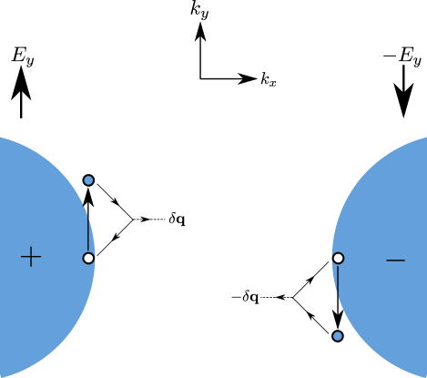
Figure 3: Elementary excitations due to the chiral electric field that carry a net chiral current at zero total momentum relative to the filled band in a two-patch system. The chiral current can decay via the emission of bosons of opposite momenta on the two patches. Since the individual bosons carry nonzero momentum, the boson distribution responds to the applied chiral electric field and is no longer in equilibrium unlike in a particle-hole symmetric system like those studied in Refs. Fritz, 2011; Patel et al., 2015, where the bosons required to relax the elementary excitations have zero momentum.

Thus, the DC chiral conductivities and hence the DC viscosities are finite and can be determined using the Boltzmann equation. Fig. 3 illustrates how chiral currents can be excited without changing the total momentum of the system. This requires oppositely directed electric fields to be applied to the two patches.

The kinetic part of the fermion Hamiltonian in the dimensionally regularized theory may be diagonalized as

$$H_{f}^{0}=\int\frac{d^{d}\mathbf{k}}{(2\pi)^{d}}\bar{\psi}(\mathbf{k})\left[i\bar{\mathbf{\Gamma}}\cdot\bar{\mathbf{K}}+i\gamma_{x}\delta_{k}\right]\psi(\mathbf{k})$$

$$=\sum_{m=\pm}\int\frac{d^{d}\mathbf{k}}{(2\pi)^{d}}m\lambda^{\dagger}_{m}(\mathbf{k})\xi(\mathbf{k})\lambda_{m}(\mathbf{k}),$$ (39)

where we use $\mathbf{k}=(k_{x},k_{y},\bar{\mathbf{K}})$, $\bar{\mathbf{K}}=(k_{1},...,k_{d-2})$ and $\bar{\mathbf{\Gamma}}=(\gamma_{1},...,\gamma_{d-2})$, with the dispersion

$$\xi(\mathbf{k})=\left(\bar{\mathbf{K}}^{2}+\delta_{k}^{2}\right)^{1/2}.$$ (40)

The $y$-component of the chiral current density becomes

$$J_{y}=\left(\sum_{m=\pm}\int\frac{d^{d}\mathbf{k}}{(2\pi)^{d}}\frac{m\delta_{k}\partial_{k_{y}}\delta_{k}}{\sqrt{\bar{\mathbf{K}}^{2}+\delta_{k}^{2}}}\lambda^{\dagger}_{m}(\mathbf{k})\lambda_{m}(\mathbf{k})\right)+J_{y}^{II},$$ (41)

where $J_{y}^{II}$ contains particle-hole terms $\lambda^{\dagger}_{+}\lambda_{-},~{}\lambda^{\dagger}_{-}\lambda_{+}$ that are unimportant for transport in the DC regime of interest Fritz et al. (2008); Fritz (2011). Defining the non-equilibrium on-shell fermion distribution functions

$$f_{f}^{m}(t,\mathbf{k})=\langle\lambda^{\dagger}_{m}(t,\mathbf{k})\lambda_{m}(t,\mathbf{k})\rangle,$$ (42)

and the non-equilibrium off-shell boson distribution function $f_{b}(t,\mathbf{q},\Omega)$, we can write down the following collision equations in presence of an applied chiral electric field $\mathbf{E}$ Kamenev (2011); Fritz (2011); Patel et al. (2015):

$$\left(\frac{\partial}{\partial t}+\mathbf{E}\cdot\frac{\partial}{\partial\mathbf{p}}\right)f_{f}^{m}(\mathbf{p},t)=-e^{2}\mu^{\epsilon}\sum_{m^{\prime}=\pm}\int\frac{d^{d}\mathbf{q}}{(2\pi)^{d}}M_{mm^{\prime}}(\mathbf{p},\mathbf{q})\mathrm{Im}\left[D^{R}(\mathbf{p}-\mathbf{q},m\xi(\mathbf{p})-m^{\prime}\xi(\mathbf{q}))\right]$$

$$\times\Big{\{}f_{f}^{m}(t,\mathbf{p})(1-f_{f}^{m^{\prime}}(t,\mathbf{q}))+f_{b}(t,\mathbf{p}-\mathbf{q},m\xi(\mathbf{p})-m^{\prime}\xi(\mathbf{q}))(f_{f}^{m}(t,\mathbf{p})-f_{f}^{m^{\prime}}(t,\mathbf{q}))\Big{\}},$$ (43)

$$\left[\frac{\partial}{\partial\Omega}(2\Omega^{2}-\mathrm{Re}[\Sigma_{b}^{R}(t,\mathbf{q},\Omega)])\frac{\partial}{\partial t}+\frac{\partial\mathrm{Re}[\Sigma_{b}^{R}(t,\mathbf{q},\Omega)]}{\partial t}\frac{\partial}{\partial\Omega}\right]f_{b}(t,\mathbf{q},\Omega)=$$

$$4\pi e^{2}\mu^{\epsilon}\sum_{m,m^{\prime}=\pm}\int\frac{d^{d}\mathbf{k}}{(2\pi)^{d}}M_{mm^{\prime}}(\mathbf{k}+\mathbf{q},\mathbf{k})\delta(m\xi(\mathbf{k}+\mathbf{q})-m^{\prime}\xi(\mathbf{k})-\Omega)\Bigg{[}f_{f}^{m}(t,\mathbf{k}+\mathbf{q})(1-f_{f}^{m^{\prime}}(t,\mathbf{k}))$$

$$+f_{b}(t,\mathbf{q},\Omega)(f_{f}^{m}(t,\mathbf{k}+\mathbf{q})-f_{f}^{m^{\prime}}(t,\mathbf{k}))\Bigg{]},$$ (44)

where the interaction matrix elements are

$$M_{mm^{\prime}}(\mathbf{p},\mathbf{q})=\frac{1}{2}\left(1+mm^{\prime}\frac{\delta_{p}\delta_{q}-\bar{\mathbf{P}}\cdot\bar{\mathbf{Q}}}{\xi(\mathbf{p})\xi(\mathbf{q})}\right)$$ (45)

(Note that $M_{++}=M_{--}$, $M_{+-}=M_{-+}$ and $M_{mm^{\prime}}(\mathbf{p},\mathbf{q})=M_{mm^{\prime}}(\mathbf{q},\mathbf{p})$), and

$$D^{R}(\mathbf{k},\omega)=\frac{|k_{y}|}{|k_{y}|^{3}+\beta_{d}e^{2}\mu^{\epsilon}(\bar{\mathbf{K}}^{2}-\omega^{2})^{(d-1)/2}},$$ (46)

where $\beta_{d}$ depends only on $d$ and is free of poles in $\epsilon$ Dalidovich and Lee (2013). The additional self-energy component appearing in the boson collision equation is given by Patel et al. (2015)

$$\mathrm{Re}[\Sigma_{b}^{R}(t,\mathbf{q},\Omega)]=-2e^{2}\mu^{\epsilon}\sum_{mm^{\prime}=\pm}\int\frac{d^{d}\mathbf{k}}{(2\pi)^{d}}M_{mm^{\prime}}(\mathbf{k},\mathbf{k}+\mathbf{q})\frac{f_{f}^{m^{\prime}}(t,\mathbf{k}+\mathbf{q})-f_{f}^{m}(t,\mathbf{k})}{m\xi(\mathbf{k})-m^{\prime}\xi(\mathbf{k}+\mathbf{q})+\Omega}.$$ (47)

Both collision integrals vanish regardless of what $D^{R}$ is when the equilibrium distributions are used due to the identity

$$n_{f}(x)(1-n_{f}(y))+n_{b}(x-y)(n_{f}(x)-n_{f}(y))=0.$$ (48)

We parameterize the deviations of the distributions from equilibrium in frequency space

$$f_{f}^{m}(\omega,\mathbf{p})=2\pi\delta(\omega)n_{f}(m\xi(\mathbf{p}))-Tn_{f}^{\prime}(\xi(\mathbf{p}))\varphi^{m}(\omega,\delta_{p},\bar{\mathbf{P}})\mathbf{E}(\omega)\cdot\mathbf{\nabla_{p}}\xi(\mathbf{p}),$$

$$f_{b}(\omega,\mathbf{q},\Omega)=2\pi\delta(\omega)n_{b}(\Omega)+u(\omega,\mathbf{q},\Omega)|\mathbf{E}(\omega)|.$$ (49)

Using these, we linearize the collision equations with $\mathbf{E}=E_{y}\hat{e}_{y}$ as we are interested in $J_{y}$. In the DC limit, we obtain (since $\lim_{\omega\rightarrow 0}(-i\omega+0^{+})\varphi^{m}(\omega,\delta_{p},\bar{\mathbf{P}})$ and $\lim_{\omega\rightarrow 0}(-i\omega+0^{+})u(\omega,\mathbf{q},\Omega)$ are expected to vanish in the presence of interactions)

$$\frac{2m\delta_{p}\sqrt{d-1}p_{y}}{\xi(\mathbf{p})}n_{f}^{\prime}(\xi(\mathbf{p}))=-e^{2}\mu^{\epsilon}\sum_{m^{\prime}=\pm}\int\frac{d^{d}\mathbf{q}}{(2\pi)^{d}}M_{mm^{\prime}}(\mathbf{p},\mathbf{q})\mathrm{Im}\left[D^{R}(\mathbf{p}-\mathbf{q},m\xi(\mathbf{p})-m^{\prime}\xi(\mathbf{q}))\right]$$

$$\times\Big{\{}\frac{2\delta_{q}\sqrt{d-1}q_{y}}{\xi(\mathbf{q})}\varphi^{m^{\prime}}(\delta_{q},\bar{\mathbf{Q}})Tn_{f}^{\prime}(\xi(\mathbf{q}))n_{f}(m\xi(\mathbf{p}))-\frac{2\delta_{p}\sqrt{d-1}p_{y}}{\xi(\mathbf{p})}\varphi^{m}(\delta_{p},\bar{\mathbf{P}})Tn_{f}^{\prime}(\xi(\mathbf{p}))(1-n_{f}(m^{\prime}\xi(\mathbf{q})))$$

$$+n_{b}(m\xi(\mathbf{p})-m^{\prime}\xi(\mathbf{q}))\left(\frac{2\delta_{q}\sqrt{d-1}q_{y}}{\xi(\mathbf{q})}\varphi^{m^{\prime}}(\delta_{q},\bar{\mathbf{Q}})Tn_{f}^{\prime}(\xi(\mathbf{q}))-\frac{2\delta_{p}\sqrt{d-1}p_{y}}{\xi(\mathbf{p})}\varphi^{m}(\delta_{p},\bar{\mathbf{P}})Tn_{f}^{\prime}(\xi(\mathbf{p}))\right)$$

$$+\mathrm{sgn}(E_{y})u(\mathbf{p}-\mathbf{q},m\xi(\mathbf{p})-m^{\prime}\xi(\mathbf{q}))(n_{f}(m\xi(\mathbf{p}))-n_{f}(m^{\prime}\xi(\mathbf{q})))\Big{\}}.$$ (50)

where we have suppressed the now zero frequency argument on the $\varphi$’s and $u$’s. For the boson collision equation we obtain

$$u(\mathbf{q},\Omega)=\mathrm{sgn}(E_{y})\frac{I_{1}[\varphi,\mathbf{q},\Omega]}{I_{2}(\mathbf{q},\Omega)},$$

$$I_{1}[\varphi,\mathbf{q},\Omega]=4\pi e^{2}\mu^{\epsilon}\sum_{mm^{\prime}=\pm}\int\frac{d^{d}\mathbf{k}}{(2\pi)^{d}}M_{mm^{\prime}}(\mathbf{k}+\mathbf{q},\mathbf{k})\delta(m\xi(\mathbf{k}+\mathbf{q})-m^{\prime}\xi(\mathbf{k})-\Omega)$$

$$\times\Bigg{[}\Big{\{}\frac{2\delta_{k}\sqrt{d-1}k_{y}}{\xi(\mathbf{k})}\varphi^{m^{\prime}}(\delta_{k},\bar{\mathbf{K}})Tn_{f}^{\prime}(\xi(\mathbf{k}))n_{f}(m\xi(\mathbf{k}+\mathbf{q}))$$

$$-\frac{2\delta_{k+q}\sqrt{d-1}(k_{y}+q_{y})}{\xi(\mathbf{k}+\mathbf{q})}\varphi^{m}(\delta_{k+q},\bar{\mathbf{K}}+\bar{\mathbf{Q}})Tn_{f}^{\prime}(\xi(\mathbf{k}+\mathbf{q}))(1-n_{f}(m^{\prime}\xi(\mathbf{k})))\Big{\}}$$

$$+n_{b}(\Omega)\Big{\{}\frac{2\delta_{k}\sqrt{d-1}k_{y}}{\xi(\mathbf{k})}\varphi^{m^{\prime}}(\delta_{k},\bar{\mathbf{K}})Tn_{f}^{\prime}(\xi(\mathbf{k}))-2\frac{\delta_{k+q}\sqrt{d-1}(k_{y}+q_{y})}{\xi(\mathbf{k}+\mathbf{q})}\varphi^{m}(\delta_{k+q},\bar{\mathbf{K}}+\bar{\mathbf{Q}})Tn_{f}^{\prime}(\xi(\mathbf{k}+\mathbf{q}))\Big{\}}\Bigg{]},$$

$$I_{2}(\mathbf{q},\Omega)=-4\pi e^{2}\mu^{\epsilon}\sum_{mm^{\prime}=\pm}\int\frac{d^{d}\mathbf{k}}{(2\pi)^{d}}M_{mm^{\prime}}(\mathbf{k}+\mathbf{q},\mathbf{k})\delta(m\xi(\mathbf{k}+\mathbf{q})-m^{\prime}\xi(\mathbf{k})-\Omega)$$

$$\times\Big{\{}n_{f}(m\xi(\mathbf{k}+\mathbf{q}))-n_{f}(m^{\prime}\xi(\mathbf{k}))\Big{\}}.$$ (51)

Since the driving term for the fermions in Eq. (44) is of opposite signs for the $+$ and $-$ quasiparticles, we expect $\varphi^{m}(\delta_{p},\bar{\mathbf{P}})=m\varphi(\delta_{p},\bar{\mathbf{P}})$. Then, using the properties of the matrix elements $M$ noted previously and that $n_{f,b}(x)+n_{f,b}(-x)=\pm 1$, one can see that $u$ is an odd function of $\Omega$ and hence that the same $\varphi(\delta_{k},\bar{\mathbf{K}})$ can be used to solve the collision equations for both branches of quasiparticles.

In the (convergent) boson collision integrals in Eq. (51), we shift $k_{x}\rightarrow k_{x}-\sqrt{d-1}k_{y}^{2}$ and integrate over $k_{y}$. In the (also convergent) fermion collision integral Eq. (50), after inserting $u$ derived from the boson collision equation we shift $q_{x}\rightarrow q_{x}-\sqrt{d-1}q_{y}^{2}$ followed by $q_{y}\rightarrow q_{y}+p_{y}$, and then integrate out $q_{y}$ after dividing through by $2\sqrt{d-1}p_{y}$. Terms that are odd in $q_{y}$ drop out, and we are left with

$$\frac{m\delta_{p}}{\xi(\mathbf{p})}n_{f}^{\prime}(\xi(\mathbf{p}))=-\frac{e^{2}\mu^{\epsilon}}{2}\sum_{m^{\prime}=\pm}\int\frac{d^{d-1}\mathbf{q}}{(2\pi)^{d}}\left(1+mm^{\prime}\frac{\delta_{p}q_{x}-\bar{\mathbf{P}}\cdot\bar{\mathbf{Q}}}{\xi(\mathbf{p})\sqrt{\bar{\mathbf{Q}}^{2}+q_{x}^{2}}}\right)$$

$$\times\mathrm{Im}\left[\frac{4\pi}{\sqrt{27}}\left(\beta_{d}e^{2}\mu^{\epsilon}\left((\bar{\mathbf{P}}-\bar{\mathbf{Q}})^{2}-\left(m\xi(\mathbf{p})-m^{\prime}\sqrt{\bar{\mathbf{Q}}^{2}+q_{x}^{2}}\right)^{2}\right)^{(d-1)/2}\right)^{-1/3}\right]$$

$$\times\Bigg{\{}\frac{q_{x}}{\sqrt{\bar{\mathbf{Q}}^{2}+q_{x}^{2}}}\varphi^{m^{\prime}}(q_{x},\bar{\mathbf{Q}})Tn_{f}^{\prime}\left(\sqrt{\bar{\mathbf{Q}}^{2}+q_{x}^{2}}\right)n_{f}(m\xi(\mathbf{p}))$$

$$-\frac{\delta_{p}}{\xi(\mathbf{p})}\varphi^{m}(\delta_{p},\bar{\mathbf{P}})Tn_{f}^{\prime}(\xi(\mathbf{p}))\left(1-n_{f}\left(m^{\prime}\sqrt{\bar{\mathbf{Q}}^{2}+q_{x}^{2}}\right)\right)$$

$$+n_{b}\left(m\xi(\mathbf{p})-m^{\prime}\sqrt{\bar{\mathbf{Q}}^{2}+q_{x}^{2}}\right)\left(\frac{q_{x}}{\sqrt{\bar{\mathbf{Q}}^{2}+q_{x}^{2}}}\varphi^{m^{\prime}}(q_{x},\bar{\mathbf{Q}})Tn_{f}^{\prime}\left(\sqrt{\bar{\mathbf{Q}}^{2}+q_{x}^{2}}\right)-\frac{\delta_{p}}{\xi(\mathbf{p})}\varphi^{m}(\delta_{p},\bar{\mathbf{P}})Tn_{f}^{\prime}(\xi(\mathbf{p}))\right)$$

$$-\frac{H_{1}[\varphi,\mathbf{\bar{P}}-\mathbf{\bar{Q}},m\xi(\mathbf{p})-m^{\prime}\sqrt{\bar{\mathbf{Q}}^{2}+q_{x}^{2}}]}{H_{2}(\mathbf{\bar{P}}-\mathbf{\bar{Q}},|m\xi(\mathbf{p})-m^{\prime}\sqrt{\bar{\mathbf{Q}}^{2}+q_{x}^{2}}|)}\left(n_{f}(m\xi(\mathbf{p}))-n_{f}\left(m^{\prime}\sqrt{\bar{\mathbf{Q}}^{2}+q_{x}^{2}}\right)\right)\Bigg{\}},$$ (52)

where

$$H_{1}[\varphi,\bar{\mathbf{Q}},\Omega]=\sum_{mm^{\prime}s}\int\frac{d^{d-1}\mathbf{k}}{(2\pi)^{d}}\frac{|m^{\prime}\sqrt{\bar{\mathbf{K}}^{2}+k_{x}^{2}}+\Omega|\Theta((m^{\prime}\sqrt{\bar{\mathbf{K}}^{2}+k_{x}^{2}}+\Omega)^{2}-(\bar{\mathbf{K}}+\bar{\mathbf{Q}})^{2})}{\left((m^{\prime}\sqrt{\bar{\mathbf{K}}^{2}+k_{x}^{2}}+\Omega)^{2}-(\bar{\mathbf{K}}+\bar{\mathbf{Q}})^{2}\right)^{1/2}}$$

$$\times\left(1+mm^{\prime}\frac{s\left((m^{\prime}\sqrt{\bar{\mathbf{K}}^{2}+k_{x}^{2}}+\Omega)^{2}-(\bar{\mathbf{K}}+\bar{\mathbf{Q}})^{2}\right)^{1/2}k_{x}-(\bar{\mathbf{K}}+\bar{\mathbf{Q}})\cdot\bar{\mathbf{K}}}{|m^{\prime}\sqrt{\bar{\mathbf{K}}^{2}+k_{x}^{2}}+\Omega|\sqrt{\bar{\mathbf{K}}^{2}+k_{x}^{2}}}\right)$$

$$\times\Bigg{[}\varphi^{m}(s((m^{\prime}(\bar{\mathbf{K}}^{2}+k_{x}^{2})^{1/2}+\Omega)^{2}-(\bar{\mathbf{K}}+\bar{\mathbf{Q}})^{2})^{1/2},\bar{\mathbf{K}}+\bar{\mathbf{Q}})\frac{s((m^{\prime}(\bar{\mathbf{K}}^{2}+k_{x}^{2})^{1/2}+\Omega)^{2}-(\bar{\mathbf{K}}+\bar{\mathbf{Q}})^{2})^{1/2}}{|m^{\prime}\sqrt{\bar{\mathbf{K}}^{2}+k_{x}^{2}}+\Omega|}$$

$$\times Tn_{f}^{\prime}(m^{\prime}(\bar{\mathbf{K}}^{2}+k_{x}^{2})^{1/2}+\Omega)\Big{\{}1-n_{f}(m^{\prime}(\bar{\mathbf{K}}^{2}+k_{x}^{2})^{1/2})+n_{b}(\Omega)\Big{\}}$$

$$-\varphi^{m^{\prime}}(k_{x},\bar{\mathbf{K}})\frac{k_{x}}{\sqrt{\bar{\mathbf{K}}^{2}+k_{x}^{2}}}Tn_{f}^{\prime}(m^{\prime}(\bar{\mathbf{K}}^{2}+k_{x}^{2})^{1/2})\Big{\{}n_{f}(m^{\prime}(\bar{\mathbf{K}}^{2}+k_{x}^{2})^{1/2}+\Omega)+n_{b}(\Omega)\Big{\}}\Bigg{]},$$

$$H_{2}(\bar{\mathbf{Q}},\Omega)=\sum_{mm^{\prime}s}\int\frac{d^{d-1}\mathbf{k}}{(2\pi)^{d}}\frac{|m^{\prime}\sqrt{\bar{\mathbf{K}}^{2}+k_{x}^{2}}+\Omega|\Theta((m^{\prime}\sqrt{\bar{\mathbf{K}}^{2}+k_{x}^{2}}+\Omega)^{2}-(\bar{\mathbf{K}}+\bar{\mathbf{Q}})^{2})}{\left((m^{\prime}\sqrt{\bar{\mathbf{K}}^{2}+k_{x}^{2}}+\Omega)^{2}-(\bar{\mathbf{K}}+\bar{\mathbf{Q}})^{2}\right)^{1/2}}$$

$$\times\left(1+mm^{\prime}\frac{s\left((m^{\prime}\sqrt{\bar{\mathbf{K}}^{2}+k_{x}^{2}}+\Omega)^{2}-(\bar{\mathbf{K}}+\bar{\mathbf{Q}})^{2}\right)^{1/2}k_{x}-(\bar{\mathbf{K}}+\bar{\mathbf{Q}})\cdot\bar{\mathbf{K}}}{|m^{\prime}\sqrt{\bar{\mathbf{K}}^{2}+k_{x}^{2}}+\Omega|\sqrt{\bar{\mathbf{K}}^{2}+k_{x}^{2}}}\right)$$

$$\times\left\{n_{f}\left(m^{\prime}\sqrt{\bar{\mathbf{K}}^{2}+k_{x}^{2}}+\Omega\right)-n_{f}\left(m^{\prime}\sqrt{\bar{\mathbf{K}}^{2}+k_{x}^{2}}\right)\right\}.$$ (53)

If we choose $\varphi^{m}(\delta_{p},\bar{\mathbf{P}})=\varphi(\delta_{p},\bar{\mathbf{P}})$ with $\varphi(\delta_{p},\bar{\mathbf{P}})=C(T)(\delta_{p}^{2}+\bar{\mathbf{P}}^{2})^{1/2}/\delta_{p}$, the right hand side of Eq. (52) vanishes due to the identity

$$n_{f}^{\prime}(x)(n_{f}(y)-1)+n_{f}(x)n_{f}^{\prime}(y)-n_{b}(x-y)(n_{f}^{\prime}(x)-n_{f}^{\prime}(y))=0.$$ (54)

This is the zero mode of the collision equation, and will lead to an infinite conductivity if excited. However, this mode cannot be excited by the chiral electric field as it produces the same (instead of opposite) deviation in the $+$ and $-$ quasiparticle distributions. This mode will be excited by a normal electric field, and is responsible for the infinite DC charge conductivity of the system. The modes excited by the chiral electric field obey $\varphi^{m}(\delta_{p},\bar{\mathbf{P}})=m\varphi(\delta_{p},\bar{\mathbf{P}})$ and are orthogonal to the zero mode, yielding a finite chiral conductivity (or viscosity).

We have

$$\eta\sim\sigma_{yy}=\frac{J_{y}}{E_{y}}=8(1-d)T\int dp_{y}p_{y}^{2}\int\frac{d^{d-1}\mathbf{p}}{(2\pi)^{d}}\frac{p_{x}^{2}}{\bar{\mathbf{P}}^{2}+p_{x}^{2}}n_{f}^{\prime}((\bar{\mathbf{P}}^{2}+p_{x}^{2})^{1/2})\varphi(p_{x},\bar{\mathbf{P}}),$$ (55)

where we shifted $p_{x}\rightarrow p_{x}-\sqrt{d-1}p_{y}^{2}$. Counting powers in Eq. (52), we obtain

$$\varphi(\xi(\mathbf{p}),\bar{\mathbf{P}})=\beta_{d}^{1/3}e^{-4/3}\mu^{-2\epsilon/3}T^{-2(d-1)/3-1}\tilde{\varphi}(\xi(\mathbf{p})/T,\bar{\mathbf{P}}/T).$$ (56)

Inserting this into Eq. (55) and using the fixed point values of $z^{\ast}=3/(2(d-1))$ and $e^{\ast 4/3}\propto\epsilon$ Dalidovich and Lee (2013), we have, to leading order in $\epsilon$,

$$\eta\sim\frac{1}{\epsilon}T^{-1/z+d-2}\int dp_{y}p_{y}^{2},$$ (57)

which is the expected quantum critical scaling.

If the Boltzmann analysis at this order is performed directly in $d=2$, then the collision equations are solved exactly by using the collisionless momentum-independent solution for $\varphi$, and thus collisions with the boson do not induce a finite DC viscosity. The reason for this is purely kinematic, stemming from the special structure of the patch dispersions in $d=2$ which have Galilean invariance in the $y$ direction and a constant $x$ velocity and was noted earlier in Ref. Maslov et al., 2011. The quantum critical scaling could possibly be restored by appropriately resumming contributions at higher orders in perturbation theory.

VI Conclusions

This paper has exposed the unconventional scaling of the shear viscosity in a theory with a critical Fermi surface. For the Ising-nematic QCP in $d=2$, we computed the optical and DC viscosities in an expansion in $\epsilon=5/2-d$ below the upper critical dimension, and showed that the viscosity scales differently than expected from that of a critical point with an effective reduced dimensionality of $(d-1)$-dimensional excitations transverse to the Fermi surface. As a consequence, the ratio $\eta/s$ diverges at low temperatures as $T^{-2/z}$ instead of saturating the universal bound like in other strongly-coupled field theories in the literature. We expect that this is a general phenomenon of metallic quantum critical states where hyperscaling is violated due to the presence of a critical Fermi surface, including states described by Fermi surfaces coupled to gauge fields. However, we do expect that metallic critical points associated with singular ‘hot spots’ on the Fermi surface Patel et al. (2015) will have a finite $\eta/s$, up to logarithmic factors.

Appendix A Optical viscosity: two-loop computations

The two-loop self-energy correction to the stress tensor autocorrelation function is given by

$$\begin{split}\langle T_{xy}T_{xy}\rangle_{\text{SE}}(i\omega)&=2N\int\frac{d^{d+1}k}{(2\pi)^{d+1}}k_{y}^{2}\operatorname{tr}\Bigl{(}\gamma_{x}G_{0}(k+q)\gamma_{x}G_{0}(k)\Sigma_{1}(k)G_{0}(k)\Bigr{)}\\ &=4e^{4/3}u_{\Sigma,0}\epsilon^{-1}\int\frac{d^{d+1}k}{(2\pi)^{d+1}}k_{y}^{2}\Bigl{(}\frac{\mu}{|\bm{K}|}\Bigr{)}^{2\epsilon/3}\frac{2\delta_{k}^{2}\bm{K}^{2}+\bm{K}\cdot(\bm{K}+\bm{Q})(\delta_{k}^{2}-\bm{K}^{2})}{\big{(}(\bm{K}+\bm{Q})^{2}+\delta_{k}^{2})(\bm{K}^{2}+\delta_{k}^{2})^{2}},\end{split}$$ (58)

where we only kept the pole contribution to the self-energy and set $\epsilon=0$ in the prefactor $u_{\Sigma,\epsilon=0}=(2\cdot 6^{1/3}\pi)^{-1}$. The self-energy correction can be computed using Feynman parameters. The integral is first rewritten as

$$\langle T_{xy}T_{xy}\rangle_{\text{SE}}(i\omega)=4(e^{2}\mu^{\epsilon})^{\frac{2}{3}}u_{\Sigma,0}\epsilon^{-1}\int\frac{d^{d+1}k}{(2\pi)^{d+1}}k_{y}^{2}\int_{0}^{1}\negthickspace dx\frac{1-x}{|\bm{K}|^{\frac{2\epsilon}{3}}}\frac{2\delta_{k}^{2}\bm{K}^{2}+\bm{K}\cdot(\bm{K}+\bm{Q})(\delta_{k}^{2}-\bm{K}^{2})}{\bigl{[}x(\bm{K}+\bm{Q})^{2}+(1-x)\bm{K}^{2}+\delta_{k}^{2}\bigr{]}^{3}}.$$ (59)

Eliminating $k_{y}$ from the fraction by a variable shift of $k_{x}$ and subsequent integration over $k_{x}$ yield

$$\begin{split}=\frac{\Gamma(3)}{4}(e^{2}\mu^{\epsilon})^{\frac{2}{3}}u_{\Sigma,0}\epsilon^{-1}&\int\negthickspace\frac{dk_{y}}{2\pi}k_{y}^{2}\int\frac{d^{d-1}K}{(2\pi)^{d-1}}\int_{0}^{1}\negthickspace dx\frac{1-x}{|\bm{K}|^{\frac{2\epsilon}{3}}}\times\Bigl{[}\frac{3\bm{K}^{2}+\bm{K}\cdot\bm{Q}}{\bigl{[}\bm{K}^{2}+x(2\bm{K}\cdot\bm{Q}+\bm{Q}^{2})\bigr{]}^{\frac{3}{2}}}-\frac{3\bm{K}^{2}(\bm{K}^{2}+\bm{K}\cdot\bm{Q})}{\bigl{[}\bm{K}^{2}+x(2\bm{K}\cdot\bm{Q}+\bm{Q}^{2})\bigr{]}^{\frac{5}{2}}}\Bigr{]}.\end{split}$$ (60)

Again using Feynman parameters to rewrite the products in the integrand, we obtain

$$\begin{split}=\frac{\Gamma(3)}{4\Gamma(\frac{\epsilon}{3})}&(e^{2}\mu^{\epsilon})^{\frac{2}{3}}u_{\Sigma,0}\epsilon^{-1}\int\negthickspace\frac{dk_{y}}{2\pi}k_{y}^{2}\int\frac{d^{d-1}K}{(2\pi)^{d-1}}\int_{0}^{1}\negthickspace dx\int_{0}^{1}\negthickspace dy\Bigl{[}\frac{\Gamma(\frac{9+2\epsilon}{6})}{\Gamma(\frac{3}{2})}\frac{(1-x)y^{\frac{\epsilon}{3}-1}(1-y)^{\frac{1}{2}}(3\bm{K}^{2}+\bm{K}\cdot\bm{Q})}{\bigl{[}\bm{K}^{2}+x(1-y)(2\bm{K}\cdot\bm{Q}+\bm{Q}^{2})]^{\frac{3}{2}+\frac{\epsilon}{3}}}\\ &\quad-\frac{\Gamma(\frac{15+2\epsilon}{6})}{\Gamma(\frac{5}{2})}\frac{3(1-x)y^{\frac{\epsilon}{3}-1}(1-y)^{\frac{3}{2}}\bm{K}^{2}(\bm{K}^{2}+\bm{K}\cdot\bm{Q})}{\bigl{[}\bm{K}^{2}+x(1-y)(2\bm{K}\cdot\bm{Q}+\bm{Q}^{2})\bigr{]}^{\frac{5}{2}+\frac{\epsilon}{3}}}\Bigr{]}.\end{split}$$ (61)

Completing squares in the denominator as

$$\bm{K}^{2}+x(1-y)(2\bm{K}\cdot\bm{Q}+\bm{Q}^{2})=(\bm{K}+x(1-y)\bm{Q})^{2}+x(1-y)(1-x+xy)\bm{Q}^{2},$$ (62)

shifting $\bm{K}\rightarrow\bm{K}-x(1-y)\bm{Q}$, and neglecting terms that vanish due to symmetries when performing the $\bm{K}$-integration, we obtain

$$\begin{split}=&\frac{\Gamma(3)}{4\Gamma(\frac{\epsilon}{3})}(e^{2}\mu^{\epsilon})^{\frac{2}{3}}u_{\Sigma,0}\epsilon^{-1}\int\negthickspace\frac{dk_{y}}{2\pi}k_{y}^{2}\int\frac{d^{d-1}K}{(2\pi)^{d-1}}\int_{0}^{1}\negthickspace dx\int_{0}^{1}\negthickspace dy(1-x)y^{\frac{\epsilon}{3}-1}\\ &\times\Bigl{\{}\frac{\Gamma(\frac{9+2\epsilon}{6})}{\Gamma(\frac{3}{2})}(1-y)^{\frac{1}{2}}\frac{3\bm{K}^{2}-x(1-y)(1-3x(1-y))\bm{Q}^{2}}{\bigl{[}\bm{K}^{2}+x(1-y)(1-y+xy)\bm{Q}^{2}\bigr{]}^{\frac{3}{2}+\frac{\epsilon}{3}}}\\ &\quad-\frac{\Gamma(\frac{15+2\epsilon}{6})}{\Gamma(\frac{5}{2})}\frac{3(1-y)^{\frac{3}{2}}}{\bigl{[}\bm{K}^{2}+x(1-y)(1-x+xy)\bm{Q}^{2}\bigr{]}^{\frac{5}{2}+\frac{\epsilon}{3}}}\Bigl{[}\bm{K}^{4}-x(1-y)(1-2x(1-y))\bm{K}^{2}\bm{Q}^{2}\\ &\quad\quad\quad-2x(1-y)(1-2x(1-y))(\bm{K}\cdot\bm{Q})^{2}-x^{3}(1-y)^{3}(1-x(1-y))\bm{Q}^{4}\Bigr{]}\Bigr{\}}\end{split}$$ (63)

The remaining integrals can easily be computed using Mathematica. First integrating over $\bm{K}$ and subsequently over $x$ and $y$, the pole contribution to the two-loop self-energy correction reads

$$\langle T_{xy}T_{xy}\rangle_{\text{SE}}(i\omega)=e^{4/3}\epsilon^{-1}\int\negthickspace\frac{dk_{y}}{2\pi}k_{y}^{2}|\omega|^{\frac{1}{2}-\epsilon}\Bigl{(}\frac{\mu}{|\omega|}\Bigr{)}^{2\epsilon/3}a_{\Sigma,0},$$ (64)

where $a_{\Sigma,0}=u_{\text{1Loop},0}u_{\Sigma,0}$, after setting $\epsilon$ to zero in the numerical prefactors.

Appendix B Relating conductivities and viscosities using Ward identities

The result in the main text, that the optical viscosity and optical conductivity scale in the same way, is not consistent with hyperscaling with an effectively reduced dimension. In order to substantiate this result, in the following we establish relations between the two transport quantities based on Ward identities.

The action for the patch theory of the Ising-nematic QCP in $d=2$, Eq. (11), is invariant under an emergent rotational symmetry Metlitski and Sachdev (2010),

$$\Phi(q_{0},q_{x},q_{y})\rightarrow\Phi^{\prime}(q_{0},q_{x},q_{y})=\Phi(q_{0},q_{x}-\Theta q_{y},q_{y})$$ (65)

$$\tilde{\psi}_{sj}(k_{0},k_{x},k_{y})\rightarrow\tilde{\psi}_{sj}^{\prime}(k_{0},k_{x},k_{y})=\tilde{\psi}_{sj}\Bigl{(}k_{0},k_{x}-\Theta k_{y}-s\frac{\Theta^{2}}{4},k_{y}+s\frac{\Theta}{2}\Bigr{)}.$$ (66)

We will show that this symmetry restricts the scaling behavior of transport properties as a function of frequency. Starting from this transformation law, we derive a Ward identity for the generating functional of connected correlation functions Negele and Orland (1998),

$$\mathcal{G}[\eta^{\dagger},\eta,\phi]=\operatorname{ln}Z[\eta^{\dagger},\eta,\phi]$$ (67)

$$Z[\eta^{\dagger},\eta,\phi]=\int D(\tilde{\psi}^{\dagger},\tilde{\psi})D(\Phi)e^{-S[\tilde{\psi}^{\dagger},\tilde{\psi},\Phi]-\int_{k}\sum_{s,j}(\tilde{\psi}^{\dagger}_{sj}(k)\eta_{sj}(k)+\eta^{\dagger}_{sj}(k)\tilde{\psi}_{sj}(k))-\int_{q}\Phi(-q)\phi(q)},$$ (68)

where $\eta^{(\dagger)}$ and $\phi$ are Grassmann and real source fields, respectively. Invariance under the above rotational symmetry implies

$$\mathcal{G}[\eta^{\prime\dagger},\eta^{\prime},\phi^{\prime}]=\mathcal{G}[\eta^{\dagger},\eta,\phi],$$ (69)

where the source fields transform as the physical fields. Differentiation with respect to $\Theta$ yields

$$\frac{d}{d\Theta}\mathcal{G}[\eta^{\prime\dagger},\eta^{\prime},\phi^{\prime}]=0,$$ (70)

which leads to the functional Ward identity

$$\begin{split}\int\frac{d^{3}k}{(2\pi)^{3}}\sum_{s,j}\Bigl{\{}&\Bigl{[}\bigl{(}k_{y}\partial_{k_{x}}\eta^{\dagger}_{sj}(k)-\frac{s}{2}\partial_{k_{y}}\eta^{\dagger}_{sj}(k)\bigr{)}\frac{\delta Z[\eta^{\dagger},\eta,\phi]}{\delta\eta^{\dagger}_{sj}(k)}+\bigl{(}k_{y}\partial_{k_{x}}\eta_{sj}(k)-\frac{s}{2}\partial_{k_{y}}\eta_{sj}(k)\bigr{)}\frac{\delta Z[\eta^{\dagger},\eta,\phi]}{\delta\eta_{sj}(k)}\Bigr{]}\\ &-\int_{q}q_{y}\partial_{q_{x}}\phi(q)\frac{\delta Z[\eta^{\dagger},\eta,\phi]}{\delta\phi(q)}\Bigr{\}}=0.\end{split}$$ (71)

In the following we are only interested in Ward identities for fermionic correlation functions and thus set $\phi=0$ from the outset.

As an example how this functional Ward identity restricts correlation functions, we derive the Ward identity that follows from rotational symmetry for the fermionic Green’s function. After computing suitable functional derivatives, we obtain

$$\bigl{(}p_{y}\partial_{p_{x}}-\frac{s}{2}\partial_{p_{y}}\bigr{)}\frac{\delta^{2}Z[\eta^{\dagger},\eta,0]}{\partial\eta_{sj}(p)\partial\eta^{\dagger}_{sj}(p)}\Bigl{|}_{\eta=\eta^{\dagger}=0}=-\bigl{(}p_{y}\partial_{p_{x}}-\frac{s}{2}\partial_{p_{y}}\bigr{)}G_{s}(p)=0,$$ (72)

where $G_{s}(p)$ is the full fermionic Green’s function. This is a partial differential equation for the momentum dependence of the latter. It can easily be verified that the Ward identity is fulfilled for $G_{s}(p)=G_{s}(p_{0},sp_{x}+p_{y}^{2})$, as expected.

For $q=q_{0}\bm{e}_{0}\neq 0$, the current-current correlation functions for the chiral current can be written as

$$\begin{split}\langle J_{x}(q)J_{x}(-q)\rangle&=\int\frac{d^{3}k}{(2\pi)^{3}}\int\frac{d^{3}k^{\prime}}{(2\pi)^{3}}\sum_{j,s,j^{\prime},s^{\prime}}\langle\tilde{\psi}_{js}^{\dagger}(k+q)\tilde{\psi}_{js}(k)\tilde{\psi}_{j^{\prime}s^{\prime}}^{\dagger}(k^{\prime}-q)\tilde{\psi}_{j^{\prime}s^{\prime}}(k^{\prime})\rangle\\ &=Z^{-1}\int\frac{d^{3}k}{(2\pi)^{3}}\int\frac{d^{3}k^{\prime}}{(2\pi)^{3}}\sum_{j,s,j^{\prime},s^{\prime}}\frac{\delta^{4}Z[\eta^{\dagger},\eta,0]}{\delta\eta_{js}(k+q)\delta\eta_{js}^{\dagger}(k)\delta\eta_{j^{\prime}s^{\prime}}(k^{\prime}-q)\delta\eta_{j^{\prime}s^{\prime}}^{\dagger}(k^{\prime})}\Bigr{|}_{\eta=\eta^{\dagger}=0}\end{split}$$ (73)

$$\begin{split}\langle J_{y}(q)J_{y}(-q)\rangle&=4\langle T_{xy}(q)T_{xy}(-q)\rangle\\ &=4\int\frac{d^{3}k}{(2\pi)^{3}}\int\frac{d^{3}k^{\prime}}{(2\pi)^{3}}\sum_{j,s,j^{\prime},s^{\prime}}ss^{\prime}k_{y}k_{y}^{\prime}\langle\tilde{\psi}_{js}^{\dagger}(k+q)\tilde{\psi}_{js}(k)\tilde{\psi}_{j^{\prime}s^{\prime}}^{\dagger}(k^{\prime}-q)\tilde{\psi}_{j^{\prime}s^{\prime}}(k^{\prime})\rangle\\ &=4Z^{-1}\int\frac{d^{3}k}{(2\pi)^{3}}\int\frac{d^{3}k^{\prime}}{(2\pi)^{3}}\sum_{j,s,j^{\prime},s^{\prime}}ss^{\prime}k_{y}k_{y}^{\prime}\frac{\delta^{4}Z[\eta^{\dagger},\eta,0]}{\delta\eta_{js}(k+q)\delta\eta_{js}^{\dagger}(k)\delta\eta_{j^{\prime}s^{\prime}}(k^{\prime}-q)\delta\eta_{j^{\prime}s^{\prime}}^{\dagger}(k^{\prime})}\Bigr{|}_{\eta=\eta^{\dagger}=0}.\end{split}$$ (74)

Applying functional derivatives to the functional Ward identity Eq. (71), we obtain a Ward identity for two-particle Green’s functions,

$$\bigl{[}(k_{y}\partial_{k_{x}}-\frac{s}{2}\partial_{k_{y}})+(k_{y}^{\prime}\partial_{k_{x}^{\prime}}-\frac{s^{\prime}}{2}\partial_{k_{y}^{\prime}})\bigr{]}\frac{\delta^{4}Z[\eta^{\dagger},\eta,0]}{\delta\eta_{js}(k+q)\delta\eta_{js}^{\dagger}(k)\delta\eta_{j^{\prime}s^{\prime}}(k^{\prime}-q)\delta\eta_{j^{\prime}s^{\prime}}^{\dagger}(k^{\prime})}\Bigr{|}_{\eta=\eta^{\dagger}=0}=0.$$ (75)

Using the method of characteristics, we can show that this Ward identity restricts the dependence of two-particle Green’s function on spatial momenta as

$$\frac{\delta^{4}Z[\eta^{\dagger},\eta,0]}{\delta\eta_{js}(k+q)\delta\eta_{js}^{\dagger}(k)\delta\eta_{j^{\prime}s^{\prime}}(k^{\prime}-q)\delta\eta_{j^{\prime}s^{\prime}}^{\dagger}(k^{\prime})}\Bigr{|}_{\eta=\eta^{\dagger}=0}=F_{js;j^{\prime}s^{\prime}}(k_{0},k_{0}^{\prime},q_{0};sk_{x}+k_{y}^{2},s^{\prime}k_{x}^{\prime}+k_{y}^{\prime 2},s^{\prime}k_{y}-sk_{y}^{\prime}),$$ (76)

analogously to the Ward identity for the one-particle Green’s function.

Inserting this result in Eqs. (73) and (74), shifting and renaming integration variables, we obtain for the $J_{x}$ correlator

$$\langle J_{x}(q_{0})J_{x}(-q_{0})\rangle =Z^{-1}\int\frac{d^{3}k}{(2\pi)^{3}}\int\frac{d^{3}k^{\prime}}{(2\pi)^{3}}\sum_{j,s,j^{\prime},s^{\prime}}F_{js;j^{\prime}s^{\prime}}(k_{0},k_{0}^{\prime},q_{0};sk_{x}+k_{y}^{2},s^{\prime}k_{x}^{\prime}+k_{y}^{\prime 2},s^{\prime}k_{y}-sk_{y}^{\prime})$$

$$=Z^{-1}\int\frac{d^{3}k}{(2\pi)^{3}}\int\frac{d^{3}k^{\prime}}{(2\pi)^{3}}\sum_{j,s,j^{\prime},s^{\prime}}F_{js;j^{\prime}s^{\prime}}(k_{0},k_{0}^{\prime},q_{0};k_{x},k_{x}^{\prime},k_{y}).$$ (77)

Note that $k_{y}^{\prime}$ does not appear in the integrand. For the $J_{y}$ correlator we obtain

$$\langle J_{y}(q_{0})J_{y}(-q_{0})\rangle =4Z^{-1}\int\frac{d^{3}k}{(2\pi)^{3}}\int\frac{d^{3}k^{\prime}}{(2\pi)^{3}}\sum_{j,s,j^{\prime},s^{\prime}}ss^{\prime}k_{y}k_{y}^{\prime}F_{js;j^{\prime}s^{\prime}}(k_{0},k_{0}^{\prime},q_{0};sk_{x}+k_{y}^{2},s^{\prime}k_{x}^{\prime}+k_{y}^{\prime 2},s^{\prime}k_{y}-sk_{y}^{\prime})$$

$$=4Z^{-1}\int\frac{d^{3}k}{(2\pi)^{3}}\int\frac{d^{3}k^{\prime}}{(2\pi)^{3}}\sum_{j,s,j^{\prime},s^{\prime}}k_{y}k_{y}^{\prime}F_{js;j^{\prime}s^{\prime}}(k_{0},k_{0}^{\prime},q_{0};k_{x},k_{x}^{\prime},k_{y}-k_{y}^{\prime})$$

$$=2Z^{-1}\int\frac{d^{3}k}{(2\pi)^{3}}\int\frac{d^{3}k^{\prime}}{(2\pi)^{3}}\sum_{j,s,j^{\prime},s^{\prime}}(k_{y}+k_{y}^{\prime})k_{y}^{\prime}F_{js;j^{\prime}s^{\prime}}(k_{0},k_{0}^{\prime},q_{0};k_{x},k_{x}^{\prime},k_{y})$$

$$\quad+2Z^{-1}\int\frac{d^{3}k}{(2\pi)^{3}}\int\frac{d^{3}k^{\prime}}{(2\pi)^{3}}\sum_{j,s,j^{\prime},s^{\prime}}k_{y}(k_{y}+k_{y}^{\prime})F_{js;j^{\prime}s^{\prime}}(k_{0},k_{0}^{\prime},q_{0};k_{x},k_{x}^{\prime},-k_{y}^{\prime})$$ (78)

where in the last step we shifted $k_{y}\rightarrow k_{y}+k_{y}^{\prime}$ and $k_{y}^{\prime}\rightarrow k_{y}^{\prime}+k_{y}$ in the first and second term, respectively. Replacing $k_{y}^{\prime}\rightarrow-k_{y}^{\prime}$ and subsequently renaming $k_{y}\leftrightarrow k_{y}^{\prime}$ in the second term, the contributions $\sim k_{y}k_{y}^{\prime}$ cancel and we hence obtain

$$=4Z^{-1}\int\frac{d^{3}k}{(2\pi)^{3}}\int\frac{d^{3}k^{\prime}}{(2\pi)^{3}}\sum_{j,s,j^{\prime},s^{\prime}}k_{y}^{\prime 2}F_{js;j^{\prime}s^{\prime}}(k_{0},k_{0}^{\prime},q_{0};k_{x},k_{x}^{\prime},k_{y}).$$ (79)

Using the Ward identity for the emergent rotational symmetry of the patch theory, we have thus established that

$$\langle J_{x}(q_{0})J_{x}(-q_{0})\rangle=\frac{\int\frac{dk_{y}}{(2\pi)}}{4\int\frac{dk_{y}}{(2\pi)}k_{y}^{2}}\langle J_{y}(q_{0})J_{y}(-q_{0})\rangle=\frac{\int\frac{dk_{y}}{(2\pi)}}{\int\frac{dk_{y}}{(2\pi)}k_{y}^{2}}\langle T_{xy}(q_{0})T_{xy}(-q_{0})\rangle.$$ (80)

As the Ward identity imposes restrictions only on the momentum dependence of the two-particle Green’s function, this result is also valid in $d=5/2-\epsilon$. The above result implies that the optical viscosity and the optical (chiral) conductivity have the same frequency dependence,

$$\sigma(\omega)\sim\eta(\omega).$$ (81)

Using the results from Ref. Eberlein et al., 2016, we obtain

$$\sigma(\omega)\sim\eta(\omega)\sim\omega^{-1/2-\epsilon/3}\stackrel{{\scriptstyle\epsilon=1/2}}{{=}}\omega^{-2/3},$$ (82)

in agreement with the field theoretic result in Eq. (33).

Appendix C Contributions from the full Fermi surface

The result Eq. (82) for the scaling of the optical viscosity was derived in the patch theory. The question arises whether the scaling could be different for the full Fermi surface, for example due to some preferred direction. In this section we show that this is not the case, using $d=2$ for simplicity.

We first analyze how the $T_{xy}$ correlator transforms under the emergent rotation symmetry of the patch theory Metlitski and Sachdev (2010). In $d=2$, $T_{xy}$ is given by

$$T_{xy}(q)=\sum_{j,s,s^{\prime}}\int_{k}\Bigl{(}k_{y}+\frac{q_{y}}{2}\Bigr{)}\tilde{\psi}_{sj}^{\dagger}(k+q)\sigma_{z,ss^{\prime}}\tilde{\psi}_{s^{\prime}j}(k).$$ (83)

We obtain

$$\langle T_{xy}T_{xy}\rangle_{\text{1Loop}}(q)\stackrel{{\scriptstyle q=\omega\bm{e}_{0}}}{{=}}-N\int_{k}k_{y}^{2}\operatorname{tr}\bigl{(}G_{0}(k_{0}+\omega,\bm{k})G_{0}(k_{0},\bm{k})\bigr{)}$$ (84)

for the correlation function, where we exploited in the last step that $G_{0}$ and $\sigma_{z}$ commute. Rotation of the Fermi momentum, with respect to which the patch theory is defined, by a small angle $\theta$ yields

$$\langle T_{xy}T_{xy}\rangle_{\text{1Loop}}(q)=-N\int_{k}\sum_{s}\Bigl{(}k_{y}+s\frac{\theta}{2}\Bigr{)}^{2}G_{0,s}(k_{0}+\omega,\bm{k})G_{0,s}(k_{0},\bm{k}),$$ (85)

where

$$k_{x} \rightarrow k_{x}-\theta k_{y}-s\frac{\theta^{2}}{4}, k_{y} \rightarrow k_{y}+s\frac{\theta}{2}.$$ (86)

The Green’s functions are independent of $\theta$ due to the emergent rotation symmetry. We can therefore eliminate $k_{y}$ from the Green’s functions by shifting $k_{x}\rightarrow k_{x}-sk_{y}^{2}$. Then $\theta$ only appears in the integrand of the $k_{y}$ integral, which is just a multiplicative prefactor, and can be eliminated by shifting $k_{y}\rightarrow k_{y}-s\frac{\theta}{2}$. Nearby patches thus contribute equally to the $T_{xy}$ correlator.

This result can be complemented by an analysis of the stress tensor correlation function for a continuum model. For an isotropic system we can start from the Lagrangian

$$\mathcal{L}(x)=\psi^{\dagger}(x)\partial_{\tau}\psi(x)+\bm{\nabla}\psi^{\dagger}(x)\cdot\bm{\nabla}\psi(x)-\mu\psi^{\dagger}(x)\psi(x),$$ (87)

where we omitted the interaction and the bosonic contribution. The $xy$-component of the stress tensor reads

$$T_{xy}(q)=\int_{k}\bigl{(}(k_{x}+q_{x})k_{y}+(k_{y}+q_{y})k_{x}\bigr{)}\psi^{\dagger}(k+q)\psi(k).$$ (88)

At one-loop level, the $T_{xy}$ autocorrelation function for $\bm{q}=0$ is then given by

$$\langle T_{xy}T_{xy}\rangle_{\text{1Loop}}(i\omega)=-4\int_{k}k_{x}^{2}k_{y}^{2}G_{0}(k+q)G_{0}(k)$$ (89)

where $q=\omega\bm{e}_{0}$.

We can subdivide the vicinity of the Fermi surface into (finite) patches, which are labeled by $\phi$, and obtain

$$\langle T_{xy}T_{xy}\rangle_{\text{1Loop}}(i\omega)=-4\sum_{\text{Patches}}\int_{k^{\prime}}(k_{x}^{\prime}\cos\phi-k_{y}^{\prime}\sin\phi)^{2}(k_{x}^{\prime}\sin\phi+k_{y}^{\prime}\cos\phi)^{2}\operatorname{tr}\bigl{(}G_{0}(k_{0}^{\prime}+\omega,\bm{k}^{\prime})G_{0}(k_{0}^{\prime},\bm{k}^{\prime})\bigr{)},$$ (90)

where the integral over $\bm{k}^{\prime}$ is over a specific patch. The sum over patches (or $\phi$-integration) sums up the contributions from individual patches. The Green’s functions do not depend on $\phi$ because they are the same in each local patch coordinate system (Fig. 4) and are just given by the patch theory action in the supplement. Shifting $k_{x}^{\prime}\rightarrow k_{F}+k_{x}^{\prime}$ in order to make the Fermi momentum explicit, we obtain

$$(k_{x}^{\prime}\cos\phi-k_{y}^{\prime}\sin\phi)^{2} (k_{x}^{\prime}\sin\phi+k_{y}^{\prime}\cos\phi)^{2}\rightarrow\frac{1}{4}\left(2k_{F}k_{y}^{\prime}\cos(2\phi)+k_{F}^{2}\sin(2\phi)-{k_{y}^{\prime}}^{2}\sin(2\phi)\right)^{2}$$

$$+\frac{1}{4}{k_{x}^{\prime}}^{2}\left(6k_{F}k_{y}^{\prime}\sin(4\phi)+6k_{F}^{2}\sin^{2}(2\phi)+{k_{y}^{\prime}}^{2}(3\cos(4\phi)+1)\right)$$

$$+\frac{1}{2}k_{x}^{\prime}\Big{(}3k_{F}^{2}k_{y}^{\prime}\sin(4\phi)+k_{F}{k_{y}^{\prime}}^{2}(3\cos(4\phi)+1)+2k_{F}^{3}\sin^{2}(2\phi)-{k_{y}^{\prime}}^{3}\sin(4\phi)\Big{)}$$

$$+{k_{x}^{\prime}}^{3}\sin(2\phi)\left(k_{F}\sin(2\phi)+k_{y}^{\prime}\cos(2\phi)\right)+{k_{x}^{\prime}}^{4}\sin^{2}\phi\cos^{2}\phi.$$ (91)

The terms in the first line of the right hand side do not depend on $k_{x}^{\prime}$ and yield the scaling that we determined from the patch theory as $k_{y}^{\prime}$ and $k_{F}$ do not scale. The terms on the other lines contain additional powers of $k_{x}^{\prime}\sim\omega^{1/z}$ and are hence subleading.

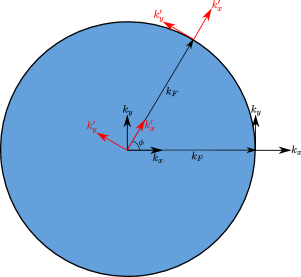
Figure 4: Transformation of coordinates used to determine the contribution of different patches to the $T_{xy}$ - $T_{xy}$ correlator.

The above argument takes care of the 1-loop and self-energy corrections. In the vertex corrections, the additional powers of $k_{x}^{\prime}$ and $k_{y}^{\prime}$ do not influence the absence of poles in $\epsilon^{-1}$. Hence all patches contribute the same scaling at leading order in $\omega$.

The expressions in Eqs. (84) and (89) are directly related only for the patches in the $k_{x}$ or the $k_{y}$ direction. In the former case, evaluating the factor $k_{x}^{2}k_{y}^{2}$ in the integrand close to the Fermi surface yields $(k_{F}+k_{x}^{\prime})^{2}{k_{y}^{\prime}}^{2}\approx k_{F}^{2}{k_{y}^{\prime}}^{2}$. After rescaling of momentum variables, this yields the factor of $k_{y}^{2}$ that appears in the stress tensor correlation function of the patch theory in Eq. (84). For other directions additional terms appear, which are not present in the patch theory, for example terms in Eq. (91) which are proportional to $k_{F}^{4}$. As $k_{F}$ and $k_{y}$ do not scale, such terms are equally relevant to the terms that appear in the patch theory and thus do not change the scaling behavior. The argument employing the emergent rotational symmetry does not generate such terms, but nevertheless leads to the correct scaling behavior.