MUSE searches for galaxies near very metal-poor gas clouds at $z\sim 3$: new constraints for cold accretion models

Abstract

We report on the search for galaxies in the proximity of two very metal-poor gas clouds at $z\sim 3$ towards the quasar Q0956$+$122. With a 5-hour MUSE integration in a $\sim 500\times 500$ kpc² region centred at the quasar position, we achieve a $\geq 80\%$ complete spectroscopic survey of continuum-detected galaxies with $m_{R}\leq 25$ mag and Ly$\alpha$ emitters with luminosity $L_{\rm Ly\alpha}\geq 3\times 10^{41}~{}\rm erg~{}s^{-1}$. We do not identify galaxies at the redshift of a $z\sim 3.2$ Lyman limit system (LLS) with $\log Z/Z_{\odot}=-3.35\pm 0.05$, placing this gas cloud in the intergalactic medium or circumgalactic medium of a galaxy below our sensitivity limits. Conversely, we detect five Ly$\alpha$ emitters at the redshift of a pristine $z\sim 3.1$ LLS with $\log Z/Z_{\odot}\leq-3.8$, while $\sim 0.4$ sources were expected given the $z\sim 3$ Ly$\alpha$ luminosity function. Both this high detection rate and the fact that at least three emitters appear aligned in projection with the LLS suggest that this pristine cloud is tracing a gas filament that is feeding one or multiple galaxies. Our observations uncover two different environments for metal-poor LLSs, implying a complex link between these absorbers and galaxy halos, which ongoing MUSE surveys will soon explore in detail. Moreover, in agreement with recent MUSE observations, we detected a $\sim 90~{}\rm kpc$ Ly$\alpha$ nebula at the quasar redshift and three Ly$\alpha$ emitters reminiscent of a “dark galaxy” population.

1 Introduction

The assembly and growth of galaxies throughout cosmic times requires the continuous accretion of substantial amounts of fresh fuel. Observations of molecular or atomic gas in the interstellar medium of both high-redshift systems and nearby galaxies reveal that, without accretion rates that are at least commensurable with the observed star formation rates (SFRs), galaxies would exhaust their gas reservoirs on timescales of $\sim 1-2~{}\rm Gyr$, much shorter than the Hubble time (e.g., Sancisi et al., 2008; Genzel et al., 2010). From this consideration, it follows that the accretion of gas from the halo (i.e. the circumgalactic medium or CGM) and, ultimately, from the baryon reservoir present in the intergalactic medium (IGM), needs to be ubiquitous at all redshifts.

In support of this argument, modern cosmological simulations predict accretions rates of $\gtrsim 10-20~{}\rm M_{\odot}~{}yr^{-1}$ at $z\sim 2-3$ galaxies (e.g., Dekel et al., 2009; Kereš et al., 2009; Faucher-Giguère et al., 2011). However, despite a general consensus that gas accretion is a dominant process for galaxy evolution, direct observational evidence of cold gas infalling onto galaxies is scarce at $z\sim 1$ (Rubin et al., 2012; Martin et al., 2012) and even more tenuous at higher redshifts (e.g., Crighton et al., 2013; Bouché et al., 2013; Martin et al., 2015). While in apparent contradiction with expectations of ubiquitous inflows, the lack of direct detections is often justified in the context of the so-called “cold stream” or “cold flow” paradigm if a significant fraction of the gas is accreted along narrow and dense filaments of cold gas (e.g., Birnboim & Dekel, 2003; Kereš et al., 2005; Dekel & Birnboim, 2006). Indeed, if the infalling gas covers only a small fraction of the solid angle as seen from a galaxy (e.g., Goerdt et al., 2012), then it is natural that only a limited number of sightlines will intersect these infalling cold streams, showing redshifted absorption lines. Moreover, for typical infall velocities of $\sim 100-200~{}\rm km~{}s^{-1}$, the signature of inflows is often masked by interstellar absorption at the systemic redshifts (Rubin et al., 2012). Further, when selecting absorbers via metal lines, some ambiguity remains in separating recycled gas falling back onto galaxies from material that is being accreted from the IGM for the first time.

Due to these intrinsic limitations, observers have to resort to other, more indirect, signatures of the presence of cold gas accretion. For instance, simulations predict that accretion in the form of cold flows is a dominant contributor to the cross section of optically-thick gas ($N_{\rm HI}\geq 10^{17.2}~{}\rm cm^{-2}$) that gives rise to Lyman limit systems (LLSs) near galaxies (e.g., Faucher-Giguère & Kereš, 2011; Fumagalli et al., 2011b; van de Voort et al., 2012). While cold streams occupy only a small fraction of the solid angle seen from a galaxy, the probability to intersect these filaments in the transverse direction with background sources is higher. Indeed, simulations predict covering factors $f_{\rm c}$ for optically-thick gas within the virial radius in the range of $f_{\rm c}\sim 0.1-0.4$, although with large variations between different models (Faucher-Giguère & Kereš, 2011; Fumagalli et al., 2011b; Shen et al., 2013; Fumagalli et al., 2014a; Faucher-Giguère et al., 2015). Thus, in principle, statistical comparisons between the observed properties of LLSs near galaxies (e.g., Rudie et al., 2012; Prochaska et al., 2013) and the predictions of numerical simulations offer interesting constraints for the cold accretion paradigm (see also Lehner et al., 2013; Fumagalli et al., 2014a; Cooper et al., 2015; Fumagalli et al., 2016).

On an object by object basis, however, the lack of direct kinematic signatures of infall requires that multiple diagnostics are combined to establish whether the gas observed in absorption is potentially being accreted onto galaxies observed in emission at close projected separations. A few examples that rely on low metallicity (e.g., Ribaudo et al., 2011; Crighton et al., 2013; Lehner et al., 2013), rotational signatures (e.g., Bouché et al., 2013; Martin et al., 2015), or filamentary morphology (e.g., Cantalupo et al., 2012) can be found in the literature. Following this approach, we present in this paper a dedicated search of galaxies around two very metal-poor LLSs with $Z\lesssim 5\times 10^{-4}Z_{\odot}$. Their extremely-low metallicity is at odds with what expected for gas that has been enriched by outflows. Thus, even without direct kinematic measurements, metal-poor LLSs that reside near galaxies are among the most compelling examples of nearly chemically-pristine gas infalling for the first time inside halos. It is however worth noting that very metal poor LLSs represent only a small fraction of the parent population, with $\lesssim 20\%$ of the LLSs having $Z\lesssim 10^{-3}Z_{\odot}$ between $z\sim 2.5$ and $3.5$ (Fumagalli et al., 2016; Lehner et al., 2016).

Our observations target the field of the quasar Q0956$+$122 (a.k.a. SDSSJ095852.19$+$120245.0), which lies at a redshift $z_{\rm qso}=3.3088\pm 0.0003$ (Hewett & Wild, 2010) and hosts two strong absorption line systems along its line of sight (Fumagalli et al., 2011a): a pristine gas cloud at $z_{\rm lls,1}=3.096221\pm 0.000009$ with H i column density $\log N_{\rm HI}=17.18\pm 0.04$ and without discernible metals to a limit of $Z<10^{-3.8}~{}\rm Z_{\odot}$; and a second LLS at $z_{\rm lls,2}=3.223194\pm 0.000002$, with column density $\log N_{\rm HI}=17.36\pm 0.05$ and metallicity $\log Z/Z_{\odot}=-3.35\pm 0.05$ (Lehner et al., 2016). A summary of the physical properties measured for these two systems or inferred via photoionization modelling by Fumagalli et al. (2011a) and Lehner et al. (2016) is presented in Table 1.

Table 1: Physical properties of the two LLSs, which are measured in absorption or inferred via photoionization modelling.

ID	$z_{\rm abs}$	$\log N_{\rm HI}$ ($\rm cm^{-2}$)	$\log Z/Z_{\odot}$	$\log n_{\rm H}$ ($\rm cm^{-3}$)	$\log x_{\rm HI}$	$\log\ell$ (pc)
LLS 1	$3.096221\pm 0.000009$	$17.18\pm 0.04$	$<-3.8$	$<-2.0$	$<-2.4$	$>3.1$
LLS 2	$3.223194\pm 0.000002$	$17.36\pm 0.05$	$-3.35\pm 0.05$	$-3.3$	$-4.1$	6.3

Details of the imaging and spectroscopic observations are presented in Section 2, followed by the analysis of continuum-detected sources and Ly$\alpha$ emitters in Section 3 and Section 4. In Section 5, we report on the discovery of an extended nebula at the quasar redshift, with discussion and conclusions in Section 6. Given the technical nature of Sections 2-4, readers who are primarily interested in the final results may prefer to continue reading from Section 5. Throughout this work, we assume solar abundances from Asplund et al. (2009) with $Z_{\odot}=0.0134$, and we use the “Planck 2013” cosmology (Planck Collaboration et al., 2014) for which the Hubble constant is $H_{0}=(67.8\pm 0.8)~{}\rm km~{}s^{-1}~{}Mpc^{-1}$ and the matter density parameter is $\Omega_{\rm m}=0.308\pm 0.010$. Magnitudes are expressed in the AB system.

2 Observations and Data Processing

2.1 Imaging observations

Imaging observations of the Q0956$+$122 field were obtained using LRIS (Oke et al., 1995) at Keck, as part of the NOAO programmes 2013A-0078 and 2013B-0102 (PI Fumagalli). Thanks to the dual-arm design of LRIS, we acquired with the D460 dichroic a 5400 s exposure using the $u^{\prime}$ filter on the blue side camera, together with a 1440 s exposure using the $V$ filter, and two 1080 s exposures in the $R$ and $I$ filters on the red side camera. Observations were conducted on UT 9 March 2013 when the target was transiting at an airmass of $\sim 1.1$ under variable conditions.

Imaging data have been processed and calibrated following the procedures described in Fumagalli et al. (2014b), including basic calibrations (bias and flat-fielding corrections), and photometric and astrometric calibrations. Due to poor seeing and patchy clouds, the resulting image quality is modest, with a point source full-width at half-maximum (FWHM) of $1.5^{\prime\prime}$ in $u^{\prime}$, $1.2^{\prime\prime}$ in $V$, $1.3^{\prime\prime}$ in $R$, and $1.3^{\prime\prime}$ in $I$. However, we recalibrate these images using the high-quality Sloan Digital Sky Survey (SDSS) photometry (Alam et al., 2015) for bright stars in the field, achieving errors on the flux calibration within $\sim 0.06-0.05$ mag for all filters. This is confirmed by the excellent agreement between $R$ band magnitudes measured in LRIS images and images reconstructed from the Multi-Unit Spectroscopic Explorer (MUSE) data collected for most part in photometric conditions (see below).

For each filter, we measure the noise properties and we extract source catalogues as described in Fumagalli et al. (2014b). For an aperture of $2^{\prime\prime}$ in diameter, we find a $2\sigma$ magnitude detection limit of $27.7$ mag in $u^{\prime}$, $26.9$ mag in $V$, $26.6$ mag in $R$, and $26.3$ mag in $I$.

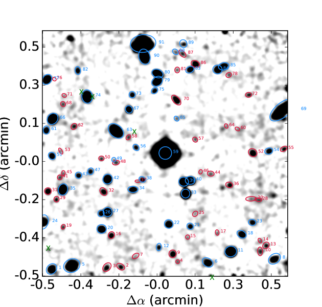
Figure 1: Image of the square region ($\sim 1.1^{\prime}$ on a side) centred at the position of Q0956$+$122, from a deep white-light image reconstructed by collapsing the MUSE datacube along the wavelength axis. The position of each continuum-detected source is marked with an aperture and the source ID. In blue, we identify sources for which a spectroscopic redshift has been measured, while in red we mark sources without spectroscopic redshifts. Green crosses mark Ly$\alpha$ emitters (see also Figure 5). Some sources are visible at the edge of the field, but they are not included in our analysis due to partial coverage or lower data quality in the periphery of the field of view.

2.2 Spectroscopic observations

High-resolution spectroscopy of the Q0956$+$122 quasar is available from the Keck HIRES archive, and the analysis of this spectrum has been presented in Fumagalli et al. (2011a) and Lehner et al. (2016).

In addition to high-resolution spectroscopy for the quasar, we have acquired integral field unit (IFU) spectroscopy within a square region of $\sim 1.1^{\prime}$ on a side centred at the quasar position. Observations have been conducted using MUSE (Bacon et al., 2010) at the UT4 Very Large Telescope (VLT) as part of the programme 094.A-0280(A) in period 94 (PI Fumagalli). Data have been acquired in Wide Field Mode using slow guiding and the extended wavelength mode to ensure non-zero throughput down to 4650 Å. A total of 4.1h on source was acquired in sets of 1500s exposures. A dither pattern with $\sim 5^{\prime\prime}$ steps and $90~{}\rm deg$ rotation was adopted to map a $68^{\prime\prime}\times 68^{\prime\prime}$ region around Q0956$+$122 with the $\sim 60^{\prime\prime}\times 60^{\prime\prime}$ MUSE field of view. With this pattern, we achieve maximum depth within the inner $40^{\prime\prime}\times 40^{\prime\prime}$, while in the outer region the sensitivity decreases radially from the quasar position. All observations were conducted in dark time, with seeing $\lesssim 0.8^{\prime\prime}$, and at airmass $<1.7$ (with an average of $\sim 1.3$) in clear or photometric conditions.

Data have been reduced using a combination of recipes from the ESO MUSE pipeline (v1.2.1; Weilbacher et al., 2014) and the CubExtractor package (CubEx in short, version 1.5; Cantalupo, in preparation), supplemented by in-house Python codes. First, we create a master bias and a master flat with the MUSE pipeline, together with a wavelength solution and an illumination correction using twilight flats. Next, we apply these calibrations to the science exposures and the standard stars used for spectro-photometric flux calibrations. Data cubes for individual exposures are constructed using a common reference grid with voxels of $1.25~{}$Å in the spectral direction and $0.2^{\prime\prime}$ in the spatial direction. At this stage, the pipeline applies a barycentric correction. Subsequently, using CubeFix and CubeSharp within the CubEx package, we improve the quality of the flat-field correction, and perform a flux-conserving sky subtraction on individual cubes (for details see, e.g., Borisova et al., 2016). The last two steps are then repeated using the cubes from the previous iteration to identify and mask sources in white-light images reconstructed from the cubes, and thus minimising the contamination from sources when computing illumination corrections. In the end, all individual exposures are combined in a final cube using mean statistics. To help with source identification, we also construct a second cube using median statistics that better rejects residual cosmic rays and artefacts in individual exposures. The wavelength calibration of MUSE data is performed in air, but we apply appropriate transformation to vacuum when comparing to HIRES data and measuring redshifts.

Before proceeding with our analysis, we also perform a series of tests on the quality of the final MUSE datacube. The final depth (root mean square) of the datacube is $5\times 10^{-19}$ $\rm erg~{}s^{-1}~{}cm^{-2}~{}\AA^{-1}~{}arcsec^{-2}$ as measured in a 10 Å window centred at 5000 Å in empty regions near the quasar position ($4\times 10^{-19}$ $\rm erg~{}s^{-1}~{}cm^{-2}~{}\AA^{-1}~{}arcsec^{-2}$ at 6000 Å). Next, we test for the absolute flux calibration by comparing the $R$-band magnitudes of sources detected in a MUSE reconstructed image against values from our deep Keck imaging, finding a difference of $<0.05$ mag in agreement with calibration errors. At this stage, we also verify the final image quality of the MUSE cubes, finding a mean FWHM of $0.67^{\prime\prime}\pm 0.02^{\prime\prime}$ for point sources. We also examine the relative flux calibration and the wavelength solution by comparing the MUSE and SDSS spectrum for the central quasar, again finding excellent agreement.

Table 2: Properties of the sources with continuum detection.

ID	R.A. (deg)	Dec. (deg)	$m_{R}$ (mag)	$m_{u^{\prime}}$ (mag)	$D_{\rm qso}$ (arcsec)	$z_{\rm spec}$	Notes
1	149.72597	12.03741	23.91$\pm$0.12	25.02$\pm$0.19	42.6	0.6502
2	149.72082	12.03758	26.13$\pm$0.40	$>$26.11	32.0	-
3	149.72184	12.03755	25.80$\pm$0.30	$>$26.65	33.6	-
4	149.71657	12.03795	26.82$\pm$0.51	$>$26.64	28.6	-
5	149.72446	12.03765	23.02$\pm$0.09	23.75$\pm$0.12	38.4	0.9456
6	149.71433	12.03789	24.60$\pm$0.19	25.26$\pm$0.25	30.6	0.8436
7	149.71970	12.03836	27.33$\pm$0.69	$>$26.65	28.0	-
8	149.70935	12.03815	24.70$\pm$0.21	24.84$\pm$0.28	39.7	1.0306
9	149.71694	12.03852	25.53$\pm$0.26	$>$26.65	26.4	-
10	149.71042	12.03869	26.11$\pm$0.35	$>$26.65	35.7	-
11	149.71261	12.03869	22.63$\pm$0.07	23.42$\pm$0.03	30.9	0.8177
12	149.71797	12.03901	26.07$\pm$0.34	$>$26.65	24.6	1.2193*	Sky residuals
13	149.70999	12.03913	26.38$\pm$0.40	$>$26.65	35.7	-
14	149.71043	12.03948	26.52$\pm$0.44	$>$26.65	33.7	-
15	149.71582	12.03973	26.82$\pm$0.51	$>$26.65	22.7	-
16	149.72151	12.03988	25.69$\pm$0.28	27.30$\pm$0.71	25.7	-
17	149.71362	12.04007	26.29$\pm$0.38	$>$26.65	24.8	-
18	149.71180	12.03994	24.88$\pm$0.19	$>$26.64	29.1	0.3391
19	149.72510	12.04049	26.44$\pm$0.39	$>$26.65	33.1	-
20	149.72223	12.04033	24.63$\pm$0.17	25.77$\pm$0.22	26.0	0.2555*	[OIII]+MgI?
21	149.71564	12.04053	25.79$\pm$0.30	$>$26.65	20.1	0.5084
22	149.71723	12.04069	24.45$\pm$0.16	$>$26.65	18.5	0.8518
23	149.71102	12.04081	25.78$\pm$0.31	26.62$\pm$0.45	29.0	1.0565
24	149.72658	12.04083	24.00$\pm$0.13	25.43$\pm$0.47	36.8	1.0058*	Sky residuals
25	149.71526	12.04143	27.06$\pm$0.59	$>$26.65	17.6	-
26	149.72228	12.04146	25.58$\pm$0.27	26.15$\pm$0.30	23.1	0.0485
27	149.72179	12.04156	23.60$\pm$0.11	26.05$\pm$0.28	21.7	0.8516
28	149.71056	12.04246	26.54$\pm$0.48	26.38$\pm$0.36	27.2	-
29	149.72560	12.04250	26.49$\pm$0.43	$>$26.65	31.1	-
30	149.71110	12.04253	26.68$\pm$0.49	27.30$\pm$0.71	25.4	-
31	149.72624	12.04309	25.23$\pm$0.23	25.67$\pm$0.27	32.5	-
32	149.72210	12.04305	25.73$\pm$0.29	26.73$\pm$0.47	19.2	-
33	149.71597	12.04290	22.46$\pm$0.06	26.46$\pm$0.38	11.8	0.0000	Star
34	149.71990	12.04321	25.09$\pm$0.22	26.98$\pm$0.57	12.8	0.0439*	H$\alpha$?
35	149.72512	12.04320	23.69$\pm$0.11	24.14$\pm$0.05	28.6	1.0847
36	149.71273	12.04354	26.08$\pm$0.35	$>$26.65	18.6	-
37	149.71955	12.04381	27.24$\pm$0.63	25.91$\pm$0.25	10.4	-
38	149.71921	12.04394	25.99$\pm$0.33	27.39$\pm$0.75	9.2	1.2003
39	149.71612	12.04377	23.46$\pm$0.10	23.72$\pm$0.04	8.8	1.0091
40	149.71563	12.04386	23.69$\pm$0.11	23.61$\pm$0.03	9.6	1.0090
41	149.72536	12.04408	26.54$\pm$0.44	26.49$\pm$0.39	28.5	-
42	149.72179	12.04396	23.83$\pm$0.12	25.38$\pm$0.16	16.7	0.8520
43	149.72396	12.04424	25.83$\pm$0.31	$>$26.65	23.6	1.1315
44	149.71410	12.04436	26.41$\pm$0.40	$>$26.64	13.0	-
45	149.72508	12.04439	27.15$\pm$0.62	$>$26.65	27.3	-
46	149.71486	12.04449	26.94$\pm$0.53	$>$26.65	10.4	-
47	149.72305	12.04453	25.85$\pm$0.31	26.78$\pm$0.48	20.2	1.0862*	Sky residuals
48	149.72116	12.04515	26.31$\pm$0.36	$>$26.65	13.3	-
49	149.72133	12.04538	26.88$\pm$0.46	$>$26.65	13.7	1.1574
50	149.72225	12.04547	26.32$\pm$0.36	$>$26.66	16.9	-

Table 3: continued

Properties of the sources with continuum detection. ID R.A. (deg) Dec. (deg) $m_{R}$ (mag) $m_{u^{\prime}}$ (mag) $D_{\rm qso}$ (arcsec) $z_{\rm spec}$ Notes 51 149.72594 12.04565 25.14$\pm$0.22 25.82$\pm$0.23 29.9 0.8051 52 149.71097 12.04589 25.39$\pm$0.25 $>$26.65 22.8 - 53 149.72528 12.04600 26.74$\pm$0.48 $>$26.65 27.6 - 54 149.70978 12.04600 25.34$\pm$0.24 $>$26.65 27.1 4.0520 55 149.70866 12.04616 26.17$\pm$0.36 26.43$\pm$0.37 31.0 - 56 149.71967 12.04626 26.18$\pm$0.35 $>$26.65 7.9 0.8506 57 149.71527 12.04683 26.89$\pm$0.51 $>$26.65 8.5 - 58 149.72025 12.04700 26.21$\pm$0.36 $>$26.65 10.7 - 59 149.71749 12.04586 17.16$\pm$0.01 20.74$\pm$0.00 0.0 3.3088 Quasar 60 149.71211 12.04761 26.90$\pm$0.59 $>$26.43 19.9 - 61 149.72636 12.04753 25.08$\pm$0.20 26.90$\pm$0.55 31.9 0.2668 62 149.72430 12.04779 26.40$\pm$0.43 $>$26.65 25.1 - 63 149.72117 12.04747 23.10$\pm$0.09 24.43$\pm$0.07 14.3 0.3752 64 149.71294 12.04782 26.87$\pm$0.53 $>$26.65 17.4 - 65 149.71665 12.04836 27.58$\pm$0.65 $>$26.65 9.5 1.5572 66 149.72590 12.04835 22.92$\pm$0.08 24.15$\pm$0.07 31.1 0.5491 67 149.72020 12.04903 24.23$\pm$0.14 $>$26.65 15.0 0.3554 68 149.72511 12.04942 26.92$\pm$0.56 $>$26.65 29.9 - 69 149.70876 12.04899 21.70$\pm$0.05 24.16$\pm$0.18 32.7 0.2710 70 149.71668 12.04971 25.12$\pm$0.21 27.19$\pm$0.65 14.2 - 71 149.72502 12.05005 $>$26.78 $>$26.65 30.7 - 72 149.71128 12.05010 26.29$\pm$0.38 $>$26.65 26.6 - 73 149.71996 12.05011 25.74$\pm$0.29 $>$26.65 17.7 0.3336 74 149.72332 12.04997 23.02$\pm$0.08 24.46$\pm$0.10 25.5 0.5556 75 149.71829 12.05040 25.86$\pm$0.29 $>$26.65 16.7 0.0740* H$\alpha$? 76 149.72576 12.05124 $>$27.39 $>$26.65 35.1 - 77 149.72631 12.05122 23.88$\pm$0.12 26.01$\pm$0.29 36.7 0.3555* Template match 78 149.71276 12.05154 26.78$\pm$0.52 $>$26.65 26.4 - 79 149.71809 12.05108 23.88$\pm$0.12 24.78$\pm$0.13 19.0 2.1311 80 149.71807 12.05165 23.47$\pm$0.10 24.99$\pm$0.13 21.0 0.5850 81 149.71660 12.05191 26.65$\pm$0.43 $>$26.65 22.1 - 82 149.72401 12.05187 25.94$\pm$0.33 26.65$\pm$0.44 31.7 1.2034 83 149.71566 12.05193 25.22$\pm$0.23 25.30$\pm$0.15 22.8 2.2912 84 149.71360 12.05194 24.64$\pm$0.17 25.14$\pm$0.13 25.8 0.5094 85 149.71313 12.05217 24.98$\pm$0.22 24.72$\pm$0.12 27.4 0.8691* MgII? 86 149.71525 12.05235 25.36$\pm$0.25 $>$26.64 24.7 - 87 149.71621 12.05310 26.65$\pm$0.45 $>$26.65 26.5 - 88 149.71673 12.05323 27.09$\pm$0.60 27.26$\pm$0.68 26.8 0.1401* H$\alpha$? 89 149.71614 12.05382 26.00$\pm$0.33 $>$26.65 29.1 4.1196* Ly$\alpha$? 90 149.71905 12.05287 22.77$\pm$0.08 23.34$\pm$0.08 26.0 0.6230 91 149.71914 12.05383 21.10$\pm$0.04 22.88$\pm$0.05 29.4 0.5562

3 Properties of continuum detected sources

3.1 Source extraction and aperture photometry

Using the MUSE median datacube, we produce a deep detection image by collapsing the cube along the wavelength axis. We then construct a source catalogue from the detection image by running sextractor (Bertin & Arnouts, 1996) with a detection area of 8 pixels and a threshold of $1.5\sigma_{\rm rms}$, where $\sigma_{\rm rms}$ is the background root mean square. Only sources within a box of $65^{\prime\prime}$ on the side ($\sim 500~{}\rm kpc$ at the redshift of the two LLSs) and centred at the quasar position are considered in the following analysis, in order to avoid spurious detections arising from edge effects and to prevent the inclusion of sources with partial coverage.

Next, using the segmentation map, we extract 1D spectra for each source from both the mean and median cubes, together with a 2D spectrum obtained by collapsing the datacube along one spatial axis. At this stage, wavelengths are shifted to vacuum for consistent redshift determinations in both HIRES and MUSE data. A list of the 91 extracted sources, detailing the positions and magnitudes of each object, is provided in Table 2. Sources are also identified within the MUSE field of view in Figure 1.

Throughout this work, we report magnitudes computed inside the Kron radius (Kron, 1980), as derived from the deep detection image. The same apertures, with appropriate astrometric transformations, are also used to extract the photometry from the Keck images. To account for the different image quality between the MUSE and Keck data, we apply a wavelength dependent aperture correction that is computed by taking the ratio of the seeing measurements in the Keck broadband images and the MUSE datacube. Agreement is found when comparing magnitudes extracted from the LRIS $R$ band image and an equivalent $R$ band image reconstructed from the MUSE datacube, providing a consistency check on both our procedures and calibrations. We emphasise, however, that while colours computed within the MUSE datacube are very robust, colours computed across instruments are more sensitive to residual offsets in the astrometric calibrations. Errors on the LRIS magnitudes are derived from the noise image following Fumagalli et al. (2014b), while errors on MUSE magnitudes are computed directly from the variance cube. These errors are used to compute upper limits for non detections, hereafter quoted at $2\sigma$ confidence level.

With $R$ band magnitudes for all the detected sources, we derive a simple metric of completeness by observing that the galaxy counts reach a peak around $m_{R}\sim 26$ mag, and steeply fall off at fainter magnitudes.

Table 4: Properties of the Ly$\alpha$ emitters near to the pristine $z\sim 3.1$ LLS.

ID	R.A. (deg)	Dec. (deg)	$\Delta v\rm(km~{}s^{-1})$	Dqso (kpc,$"$)	$F_{\rm Ly\alpha}\rm(10^{-18}erg~{}s^{-1}cm^{-2})$
1-3	149.72298	12.04986	-1149	189.5, 24.26	$5.9\pm 0.5$
1-12	149.72627	12.03883	-375	312.4, 40.00	$13.7\pm 1.1$
1-21	149.71985	12.04730	795	77.7, 9.95	$4.0\pm 0.4$
1-25	149.72380	12.05021	861	213.4, 27.32	$3.4\pm 0.4$
1-26	149.71406	12.03670	1033	273.4, 35.01	$3.6\pm 0.6$

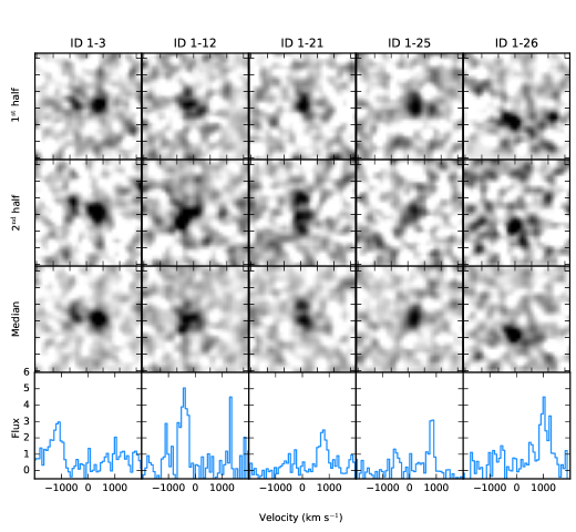
Figure 2: Gallery of the five Ly$\alpha$ emitters identified in proximity of the $z\sim 3.1$ LLS. Each emitter is shown in a column, where from top to bottom we show optimally-extracted images obtained with CubEx (Cantalupo, in preparation; see also Borisova et al., 2016) from two independent cubes each containing half of all the exposures and from the median cube. The bottom row shows the 1D spectra, with velocities relative to the LLS redshift and fluxes in units of $10^{-20}~{}\rm erg~{}s^{-1}~{}cm^{-2}~{}\AA^{-1}$.

3.2 Spectroscopic redshifts

To measure the redshift of the continuum detected sources, we first visually inspect each spectrum in 1D and 2D to search for emission and absorption lines. Weak features are confirmed by inspecting spectra from the mean and median cubes. When multiple absorption and emission lines are identified, we determine redshifts from Gaussian fits to the emission lines, with typical errors of $\delta z\sim 0.0002-0.0003$. For sources without emission lines, instead, we compare spectra to templates from SDSS/DR5 (Adelman-McCarthy et al., 2007) or to Lyman Break Galaxy (LBG) templates from Bielby et al. (2013) using a custom-made graphical user interface. For the few cases in which a single emission or absorption line is detected and no other strong unambiguous features are visible, we assign a tentative redshift as described in Table 2. Following these steps, we measure redshifts for $48/91$ sources ($38/91$ with robust redshifts), achieving a nearly complete spectroscopic redshift survey for sources with $m_{R}\leq 25$ mag (with $24/28$ sources having robust redshifts). A summary of redshift measurements is provided in Table 2, which reveals no association with the two LLSs.

In passing, we note the presence of a group of at least four sources at $z\sim 0.85$ (ID 22, 27, 42, 56) which is within $\sim 300~{}\rm km~{}s^{-1}$ from a Mg ii absorption system detected at $z=0.85010\pm 0.00001$. Among these sources, ID 56 lies at a projected separation of $\sim 8^{\prime\prime}$ or $\sim 60~{}\rm kpc$ from the absorption line system, at nearly coincident redshift.

3.3 Colour selection of $z\sim 3.0-3.3$ galaxies

For galaxies with $m_{R}>25$ mag for which our spectroscopic redshift survey becomes severely incomplete, we investigate with colour information whether the MUSE field of view contains galaxies with spectral energy distributions (SEDs) consistent with sources at $z\sim 3.0-3.3$. To this end, we generate observed SEDs for all the sources with continuum detection in the MUSE datacube using six photometric data points, which are extracted from the Keck $u^{\prime}$-band image and from five medium-band images from the MUSE datacube with a 500 Å wide top-hat filter centred at 4900 Å, 5400 Å, 5900 Å, 6400 Å, and 6900 Å. At this stage, we also correct the observed magnitudes for the wavelength-dependent Galactic extinction, following Schlafly & Finkbeiner (2011). For the broadband photometry reported in Table 2, these corrections are $A_{u^{\prime}}=0.15$ mag and $A_{R}=0.07$ mag.

To search for sources with colours consistent with $z\sim 3.0-3.3$ galaxies, we use the eazy code (Brammer et al., 2008). Using sources with a spectroscopic redshift as a test bed (at redshifts $z<3$), we find that our photometry does not span a sufficient wavelength range to remove the well-known degeneracy between low and high redshift sources. Moreover, and perhaps most importantly, the $u^{\prime}$-band image was acquired in modest weather conditions thus limiting the constraining power of the (weak) upper limits from the LRIS $u^{\prime}$-band image. This fact is indeed reflected by the broad redshift range spanned by the likelihood functions. For this reason, when integrating the redshift probability distribution function derived assuming a flat prior on the magnitude in the redshift interval $z=[3.0,3.3]$, we do not identify any galaxy with a significant probability excess ($\gtrsim 50\%$) in the interval of interest. Only three sources (ID 52, 53, and 86) exhibit a modest excess of $\sim 25-30\%$, but the broad shape of the posterior redshift distribution function prevents us from conclusively identifying any of them as the host of one of the two LLSs.

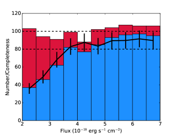
Figure 3: Results of a completeness test for the recovery of Ly$\alpha$ emitters between $z\sim 3.1$ and $3.2$. In red, we show the input mock flux distribution, and in blue we show the number of sources identified by CubEx. The black solid line shows the recovered fraction, including counting errors. Our search for Ly$\alpha$ emitters is $\geq 80\%$ complete for fluxes $\geq 3.5\times 10^{-18}~{}\rm erg~{}s^{-1}~{}cm^{-2}$.

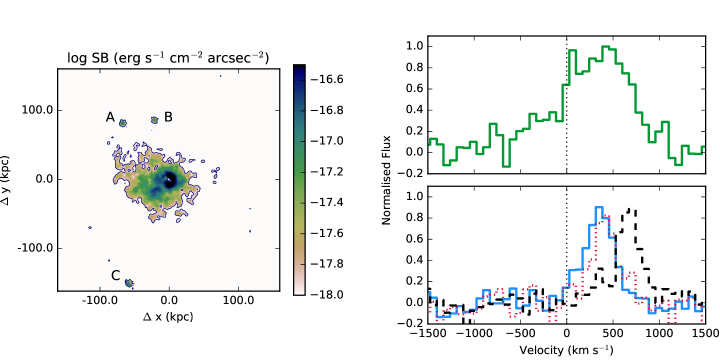
Figure 4: (Left) Ly$\alpha$ surface brightness map of an extended nebula and of three Ly$\alpha$ emitters discovered at the quasar redshift. The image shows the surface brightness derived from optimally-extracted line maps. The blue contour shows the $10^{-18}$ $\rm erg~{}s^{-1}~{}cm^{-2}~{}arcsec^{-2}$ level. (Right) Spectra integrated over the segmentation map for the extended nebula (top) and the three emitters (bottom; solid blue line for source A, red dotted line for source B, and black dashed line for source C). The velocity scale is centred at the quasar redshift derived from rest-frame UV lines (vertical dotted line).

4 Properties of line emitters

We focus next on the detection and characterisation of line emitters which, due to their faint continuum level, may be undetected in the deep white-light image. Throughout this section, we make use of the CubEx capability (Cantalupo, in preparation) of identifying sources in three dimensions by searching for groups of contiguous voxels in the MUSE datacube above a desired signal-to-noise ratio ($S/N$) threshold both in the spatial direction and along the wavelength axis.

We search for line emitters in proximity of the two intervening LLSs within a window of about $\pm 1000~{}\rm km~{}s^{-1}$, running CubEx on the mean cube, after having subtracted the quasar point spread function (PSF) and the continuum emission of each source as described in Borisova et al. (2016). To ensure the highest completeness to faint fluxes, we extract candidate sources with a minimum volume of 50 voxels at $S/N\geq 3$. At this step, the cube is convolved in the spatial direction with a boxcar filter of 2 pixels and the variance cube is rescaled by a factor of $\sim 1.8$ (weakly dependent on wavelength) to match the value measured within the datacube.

After having identified the sources, we visually inspect optimally-extracted line flux images (for details, see Borisova et al., 2016) both from the mean and median cube. To avoid the inclusion of spurious sources (e.g., cosmic rays residuals or image defects arising from the edges of the frame), we also construct line flux images from two independent cubes containing only one of the two exposures collected in each observing block. Following visual inspection, a source is included in the final catalogue if it is detected both in the mean and median cubes, as well as in the two independent cubes constructed from half of all the exposures available. While this choice affects the recovery fraction at the faint end of the flux distribution, it ensures that only reliable sources are included in the final analysis.

Finally, we extract 1D spectra and measure redshifts by fitting Gaussian functions to the emission lines. Sources are classified as Ly$\alpha$ emitters if the emission line is not resolved, which would be indicative of [OII] emission, and no positive identification of other emission lines (H$\alpha$, [OIII], H$\beta$) is made in the spectrum.

In a window of about $\pm 1000~{}\rm km~{}s^{-1}$ centred at redshift of the $z\sim 3.1$ LLS, we identify six line emitters, five of which are classified as Ly$\alpha$ sources. The remaining source is an [OII] emission line coinciding with the continuum-detected galaxy ID 18. Conversely, at the redshift of $z\sim 3.2$ LLS, we detect only one source with more than 50 voxels above $S/N=3$, which is a strong, spatially resolved, [OII] emission line associated with the galaxy ID 63 at $z\sim 0.3752$. No other sources are identified as Ly$\alpha$ emitters within this region of the cube.

For each Ly$\alpha$ emitter detected near the $z\sim 3.1$ LLS, we also measure the distance from the quasar centroid where $\rm H\,{\small I}$ absorption is detected, and we integrate the line flux within the three-dimensional segmentation maps provided by CubEx. While this choice maximises the $S/N$ of this measurement, fluxes should be regarded as formal lower limits, although we note modest differences when integrating the flux in a cubic region that encompasses the full extent of the detected emission line (see also below). A summary of the properties of the five Ly$\alpha$ emitters identified at the redshift of the $z\sim 3.1$ LLS is provided in Table 4 and Figure 2.

Finally, we assess the completeness of our search for Ly$\alpha$ emitters by means of mock tests. Specifically, we populate the mean datacube (preserving the original noise) with line emitters with fluxes in the range $(2-7)\times 10^{-18}~{}\rm erg~{}s^{-1}~{}cm^{-2}$ and size defined by a two-dimensional Gaussian with $0.7^{\prime\prime}$ FWHM in the spatial direction, and a Gaussian of 2.5 Å FWHM in the spectral direction. During this test, we inject 500 sources at the redshift of each LLS, which represents a compromise between reducing counting errors and avoiding blending of sources. We then process these mock cubes following the same analysis adopted for the real data, finding similar results for each LLS. The fraction of recovered sources combined for both LLSs is shown in Figure 3, which indicates that our search is $\geq 80\%$ complete for line fluxes $\geq 3.5\times 10^{-18}~{}\rm erg~{}s^{-1}~{}cm^{-2}$. As visible in the figure, occasional blending slightly reduces the completeness also at the bright end. At this stage, we also test the quality of the recovered line fluxes, finding that the discrepancy between the input and recovered fluxes is distributed as a Gaussian, the centre of which is consistent with zero to within the 1$\sigma$ flux errors.

5 An extended nebula associated with the quasar

Upon inspection of the datacube at wavelengths corresponding to Ly$\alpha$ at the redshift of the quasar, we identify extended diffuse emission as well as the presence of three compact emitters. After subtracting the quasar PSF and all continuum detected sources, we obtain a segmentation map for the diffuse emission by identifying with CubEx pixels with $S/N\geq 2$ inside a region of minimum area of 2000 voxels, chosen to be large enough to filter compact sources. To characterise the three emitters, we further run CubEx to search for sources composed of at least 60 voxels with $S/N\geq 5$. Figure 4 shows the surface brightness map and 1D spectra of both the nebula and these Ly$\alpha$ emitters.

As shown in the figure, this nebula is highly asymmetric and extends in the east direction for up to $\sim 12^{\prime\prime}$, or $\sim 90~{}\rm kpc$ at the redshift of the quasar, with a surface brightness of $\geq 10^{-18}~{}$$\rm erg~{}s^{-1}~{}cm^{-2}~{}arcsec^{-2}$. While not as dramatic as some of the giant nebulae uncovered around $z\sim 2$ quasars (Cantalupo et al., 2014; Hennawi et al., 2015), this nebula is brighter than the typical nebulae seen around $z\sim 2$ quasars (Arrigoni Battaia et al., 2016), and it is comparable to the nebulae seen by MUSE at $z\sim 3$ around all bright radio-quiet quasars observed so far (e.g., Borisova et al., 2016). Kinematically, the bulk of the Ly$\alpha$ emission is redshifted by $\sim 500~{}\rm km~{}s^{-1}$ when considering the quasar redshift measured from rest-frame UV lines (Figure 4, top-right panel) and spans $\gtrsim 600~{}\rm km~{}s^{-1}$ in velocity, with a second component extending to negative velocity.

The spectra of the three compact sources show prominent Ly$\alpha$ emission aligned in velocity space with the nebula (Figure 4, bottom-right panel). No obvious signatures of a strong AGN component are evident from the spectra of these compact sources. The emitters have a line flux integrated over the segmentation map of $(8.4\pm 0.4)\times 10^{-18}~{}\rm erg~{}s^{-1}~{}cm^{-2}$ (source A), $(5.1\pm 0.4)\times 10^{-18}~{}\rm erg~{}s^{-1}~{}cm^{-2}$ (source B), and $(8.9\pm 0.5)\times 10^{-18}~{}\rm erg~{}s^{-1}~{}cm^{-2}$ (source C). As previously discussed, these values represent formally lower limits, as additional flux may be present outside of the voxels selected by the segmentation map. However, we have shown that this effect is expected to be a minor one, with all the flux being recovered typically within errors. Source A is also detected in the continuum, with an $R$ band magnitude of $m_{R}=27.5\pm 0.2$ mag computed inside an aperture matched to the size of the Ly$\alpha$ emission. However, we cannot exclude contamination from the nearby source ID 67 in close proximity to emitter A, and we consider this measurement an upper limit to the actual continuum. Conversely, source B and C are not detected in the continuum within the $R$ band image, to a limiting magnitude of $28.6$ mag and $28.9$ mag ($2\sigma$) within an aperture matched to the Ly$\alpha$ emission.

With a luminosity of $L_{\rm Ly\alpha}\geq 5\times 10^{41}~{}\rm erg~{}s^{-1}$ and lacking appreciable continuum emission, these sources are characterised by equivalent widths $>100-140~{}$Å in aperture matched to the extent of the Ly$\alpha$ emission, or $>150-280~{}$Å when adopting apertures matched to the seeing of the continuum image. Thus, these sources are reminiscent of the population of bright emitters, including “dark galaxies” with equivalent widths in excess of 240 Å, reported by Cantalupo et al. (2012) around a bright quasar that boosts the Ly$\alpha$ emission intrinsic to the sources. Indeed, in a volume of $\sim 150~{}\rm Mpc^{3}$ defined by the MUSE field of view and a velocity window of $\pm 1500~{}\rm km~{}s^{-1}$ around the quasar redshift, one would expect to see approximately two emitters according to the luminosity function presented in Cantalupo et al. (2012) when including the boost due to quasar radiation. This estimate is in line with our observations and a factor of $\sim 5$ above the expectation from the field luminosity functions (e.g., Cassata et al., 2011).

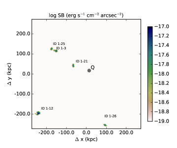
Figure 5: Spatial distribution of the Ly$\alpha$ emitters at the redshift of the $z\sim 3.1$ LLS. North is up, east to the left. The quasar position is marked by the grey circle. The alignment in projection of at least three Ly$\alpha$ emitters and a pristine LLS is suggestive of a cosmic web filament crossing the field of view in the north-east/south-west direction.

6 Discussion and Conclusions

Our analysis of a deep MUSE exposure in the field of the quasar Q0956$+$122 that hosts two very metal-poor LLSs provides a proof-of-concept of the power of IFU spectroscopy at large telescopes for addressing open questions on the nature of LLSs and their link with the CGM of galaxies as predicted by simulations (e.g., Faucher-Giguère & Kereš, 2011; Fumagalli et al., 2011b; Shen et al., 2013; Fumagalli et al., 2014a; Faucher-Giguère et al., 2015). Indeed, with a 5 hour observation, we have achieved a $\geq 80\%$ complete spectroscopic survey for continuum-detected galaxies with $m_{R}\leq 25$ mag and for Ly$\alpha$ emitters with luminosity $L_{\rm Lya}\geq 3\times 10^{41}~{}\rm erg~{}s^{-1}$. This drastically improves on what was previously possible with narrow-band or (multi-object) spectroscopic surveys (e.g., Fynbo et al., 2000; Rauch et al., 2008; Crighton et al., 2015).

In our observations, we do not identify bright continuum-detected sources at the redshift of the two LLSs, thus excluding a rapidly star-forming galaxy (i.e. a “classic” LBG) with mean halo mass $\log M/M_{\odot}\sim 11.5$ (Bielby et al., 2013) and observed SFRs of $\gtrsim 6~{}\rm M_{\odot}~{}yr^{-1}$ as the host of these gas clouds. These are the galaxies that are generally targeted in studies of galaxy-quasar pairs (e.g., Rudie et al., 2012; Prochaska et al., 2013).

Furthermore, when searching for Ly$\alpha$ emitters near the metal-poor ($\log Z/Z_{\odot}=-3.35\pm 0.05$) LLS at $z\sim 3.2$, we do not detect any source to a limiting luminosity of $L_{\rm Lya}\geq 3\times 10^{41}~{}\rm erg~{}s^{-1}$ (uncorrected for dust or IGM absorption), corresponding to SFRs of $\gtrsim 0.2~{}\rm M_{\odot}~{}yr^{-1}$ (see Rauch et al., 2008) and for which our search is $\geq 80\%$ complete. The lack of any detection of Ly$\alpha$ emitters within a comoving volume of $\sim 95~{}\rm Mpc^{-3}$ defined by the MUSE field of view and a velocity window of $\pm 1000~{}\rm km~{}s^{-1}$ is consistent with the field luminosity function at $z\sim 3$ (Grove et al., 2009; Cassata et al., 2011) according to which $\sim 0.4$ emitters should be expected above our sensitivity limit. Thus, the lack of galaxies at the redshift of this metal-poor gas cloud implies that this $z\sim 3.2$ LLS arises either from a pocket of the IGM (possibly connecting faint galaxies) or from the CGM of a galaxy below our sensitivity limit. Although it is difficult to precisely estimate the physical densities and sizes of LLSs (Fumagalli et al., 2016), we note that the IGM origin is also supported by the low density and Mpc-scale size of the absorbing cloud (see Table 1 and Lehner et al., 2016). It should be also noted that while dust is expected to play a negligible role particularly in these chemically pristine environments, we cannot exclude biases arising from extinction based only on our data.

Conversely, when searching for Ly$\alpha$ emitters at the redshift of the pristine ($Z<10^{-3.8}~{}\rm Z_{\odot}$) LLS at $z\sim 3.1$, we identify five emitters (Figure 2). Of those, ID 1-21 lies at a close impact parameter from the quasar ($D_{\rm qso}=77.7\pm 0.5~{}\rm kpc$) at a velocity separation of $\Delta v=795\pm 20~{}\rm km~{}s^{-1}$ with respect to the LLS redshift. While this velocity shift is apparently high, redshifts of $\sim 300-400~{}\rm km~{}s^{-1}$ relative to systemic are common for Ly$\alpha$ due to its resonant nature, and offsets up to $\sim 800~{}\rm km~{}s^{-1}$ have been observed (Steidel et al., 2010; Rakic et al., 2011). Thus, ID 1-21 is likely to be the closest galaxy in physical space to the pristine LLS. In velocity space, instead, ID 1-12 is the closest to the LLS without considering radiative transfer effects ($\Delta v=-375\pm 20~{}\rm km~{}s^{-1}$), but at larger projected impact parameter ($D_{\rm qso}=312.4\pm 0.5~{}\rm kpc$). For comparison, most of the host galaxies of the $z\sim 1$ LLSs that have been reported in the literature (e.g., Lehner et al., 2013) lie at distances of $\lesssim 100~{}\rm kpc$ and velocities of $\lesssim 350~{}\rm km~{}s^{-1}$.

Given that the physical three-dimensional distance from each source to the LLS is unknown, it is difficult to unambiguously identify the closest host galaxy and to directly compare to the results of simulations. However, when considered altogether, the detection of five sources in a small volume centred at the LLS redshift is an extremely rare fluctuation compared to the field number density of Ly$\alpha$ emitters. As discussed, adopting the Cassata et al. (2011) luminosity function, we should expect to detect $\sim 0.4$ emitters in this volume. Thus, the detection of five emitters corresponds to a very rare event with probability of $\sim 5\times 10^{-5}$ of occurring at random. For this reason, we conclude that the pristine LLS lies within a “rich” environment with a biased population of Ly$\alpha$ emitters, among which ID 1-21 is possibly the closest association.

Moreover, as shown in Figure 5, at least three of the detected emitters (four if including ID 1-26) appear to lie along a line which also intersects the location where the pristine LLS is detected in absorption. Given the lack of systematic correlation in the line-of-sight velocity of these emitters, and given that Ly$\alpha$ is a resonant transition, we cannot propose an unambiguous interpretation for this alignment. However, this morphology is strongly suggestive of a filament that crosses the field in the north-east/south-west direction (cf. Møller & Fynbo, 2001). This feature, in conjunction with the fact that this cloud has no detectable metals but lies at close separation from at least one galaxy, supports the idea that this LLS originates from a cold stream that connects and feeds one or multiple Ly$\alpha$ emitters with modest SFRs. As noted above, however, the assertion that this gas is infalling is only indirectly inferred from a combination of low metallicity and proximity to one or more galaxies, as we lack direct observational evidence that the gas is indeed moving towards or inside a halo. Following this argument, even if the observed alignment of sources was coincidental and solely due to projection effects, our data would nevertheless suggest a picture in which nearly-pristine gas is being accreted from the IGM inside a group of emitters.

Our work adds new constraints for the scenario put forward by modern cosmological simulations, particularly within the cold accretion paradigm (e.g., Faucher-Giguère & Kereš, 2011; Fumagalli et al., 2011b; Shen et al., 2013; Fumagalli et al., 2014a; Faucher-Giguère et al., 2015). On the one hand, the association of a metal-poor LLS with multiple Ly$\alpha$ emitters offers one of the most compelling examples of chemically-pristine gas that is likely accreting onto a galaxy (or a galaxy group), in line with theoretical predictions. On the other hand, our observations uncover two different environments for these metal-poor LLSs. This cautions against blind associations between individual very-metal poor LLSs and cold streams purely relying on absorption measurements. While not ruled out, this link needs more solid footing (see e.g., Ribaudo et al., 2011; Crighton et al., 2013; Fumagalli et al., 2016).

The fact that metal-poor LLSs should not simply be connected to accretion based on their metal content alone is also reinforced by considerations on the $\rm H\,{\small I}$ column density. Indeed, besides having very low metal content, both LLSs targeted by our observations also have a relatively low column density ($\log N_{\rm HI}=17.2-17.4$), at the limit of the threshold that defines optically-thick absorbers. With the exception of some partial LLSs, studies of large samples of absorbers at $z\sim 3$ hint at a decline in the metal distribution of optically-thick gas at low column densities and low physical densities (e.g., Cooper et al., 2015; Fumagalli et al., 2016; Glidden et al., 2016; Lehner et al., 2016), implying that metal poor absorption line systems around $\log N_{\rm HI}\sim 17$ may arise not only from CGM gas, but also from the IGM. Such a contribution from both CGM and IGM in low-column density and metal-poor LLSs would explain the different environments seen around these two LLSs, a conclusion which is also reinforced by the different densities and sizes inferred for these two absorbers (Table 1).

In summary, while we cannot draw far-reaching conclusions on the nature of LLSs and their connection to the CGM of galaxies from a single field, our observations place these two very metal poor LLSs in an environment that resembles the IGM or the CGM of galaxies with very modest SFRs in one case, and in an environment that is consistent with a cold stream feeding one or more galaxies in the second case. While our results should not be trivially extrapolated to the full LLS population because very metal poor systems represent only $\lesssim 20\%$ of the LLS population at these redshifts (Fumagalli et al., 2016; Lehner et al., 2016), our analysis provides a clear indication that the claimed connection between metal-poor LLSs and star-forming galaxies fed by cold streams is plausible, but still requires empirical scrutiny across a wide range of metallicity and column density. The answer to this open question is likely within reach in the era of large-field IFUs at 8m telescopes, thanks to dedicated observations (such as our own MUSE programme 197.A-0384(A)) that will soon target $z\sim 3.5$ quasar fields hosting $z\sim 3$ LLSs. Combined with new observations at lower redshift, these IFU surveys will also enable detailed comparisons with studies at $z\sim 1$ that currently place most of the optically-thick absorbers within $\sim 100~{}\rm kpc$ of galaxies regardless to their metallicity (e.g., Lehner et al., 2013).

References

- (1)
- Adelman-McCarthy et al. (2007) Adelman-McCarthy, J. K., Agüeros, M. A., Allam, S. S., et al. 2007, ApJS, 172, 634
- Alam et al. (2015) Alam, S., Albareti, F. D., Allende Prieto, C., et al. 2015, ApJS, 219, 12
- Arrigoni Battaia et al. (2016) Arrigoni Battaia, F., Hennawi, J. F., Cantalupo, S., & Prochaska, J. X. 2016, arXiv:1604.02942
- Asplund et al. (2009) Asplund, M., Grevesse, N., Sauval, A. J., & Scott, P. 2009, ARA&A, 47, 481
- Astropy Collaboration et al. (2013) Astropy Collaboration, Robitaille, T. P., Tollerud, E. J., et al. 2013, A&A, 558, A33
- Bacon et al. (2010) Bacon, R., Accardo, M., Adjali, L., et al. 2010, Proc. SPIE, 7735, 9
- Bertin & Arnouts (1996) Bertin, E., & Arnouts, S. 1996, A&AS, 117, 393
- Bielby et al. (2013) Bielby, R., Hill, M. D., Shanks, T., et al. 2013, MNRAS, 430, 425
- Birnboim & Dekel (2003) Birnboim, Y., & Dekel, A. 2003, MNRAS, 345, 349
- Borisova et al. (2016) Borisova, E., Cantalupo, S., Lilly, S. J., et al. 2016, arXiv:1605.01422
- Bouché et al. (2013) Bouché, N., Murphy, M. T., Kacprzak, G. G., et al. 2013, Science, 341, 50
- Brammer et al. (2008) Brammer, G. B., van Dokkum, P. G., & Coppi, P. 2008, ApJ, 686, 1503
- Cantalupo et al. (2012) Cantalupo, S., Lilly, S. J., & Haehnelt, M. G. 2012, MNRAS, 425, 1992
- Cantalupo et al. (2014) Cantalupo, S., Arrigoni-Battaia, F., Prochaska, J. X., Hennawi, J. F., & Madau, P. 2014, Nature, 506, 63
- Cassata et al. (2011) Cassata, P., Le Fèvre, O., Garilli, B., et al. 2011, A&A, 525, A143
- Cooper et al. (2015) Cooper, T. J., Simcoe, R. A., Cooksey, K. L., O’Meara, J. M., & Torrey, P. 2015, ApJ, 812, 58
- Crighton et al. (2013) Crighton, N. H. M., Hennawi, J. F., & Prochaska, J. X. 2013, ApJ, 776, L18
- Crighton et al. (2015) Crighton, N. H. M., Hennawi, J. F., Simcoe, R. A., et al. 2015, MNRAS, 446, 18
- Dekel et al. (2009) Dekel, A., Birnboim, Y., Engel, G., et al. 2009, Nature, 457, 451
- Dekel & Birnboim (2006) Dekel, A., & Birnboim, Y. 2006, MNRAS, 368, 2
- Faucher-Giguère et al. (2015) Faucher-Giguère, C.-A., Hopkins, P. F., Kereš, D., et al. 2015, MNRAS, 449, 987
- Faucher-Giguère & Kereš (2011) Faucher-Giguère, C.-A., & Kereš, D. 2011, MNRAS, 412, L118
- Faucher-Giguère et al. (2011) Faucher-Giguère, C.-A., Kereš, D., & Ma, C.-P. 2011, MNRAS, 417, 2982
- Fumagalli et al. (2014a) Fumagalli, M., Hennawi, J. F., Prochaska, J. X., et al. 2014a, ApJ, 780, 74
- Fumagalli et al. (2014b) Fumagalli, M., O’Meara, J. M., Prochaska, J. X., Kanekar, N., & Wolfe, A. M. 2014b, MNRAS, 444, 1282
- Fumagalli et al. (2011a) Fumagalli, M., O’Meara, J. M., & Prochaska, J. X. 2011a, Science, 334, 1245
- Fumagalli et al. (2011b) Fumagalli, M., Prochaska, J. X., Kasen, D., et al. 2011b, MNRAS, 418, 1796
- Fumagalli et al. (2016) Fumagalli, M., O’Meara, J. M., & Prochaska, J. X. 2016, MNRAS, 455, 4100
- Fynbo et al. (2000) Fynbo, J. U., Thomsen, B., Møller, P. 2000, A&A, 353, 457
- Genzel et al. (2010) Genzel, R., Tacconi, L. J., Gracia-Carpio, J., et al. 2010, MNRAS, 407, 2091
- Glidden et al. (2016) Glidden, A., Cooper, T. J., Cooksey, K. L., Simcoe, R. A., & O’Meara, J. M. 2016, arXiv:1604.02144
- Goerdt et al. (2012) Goerdt, T., Dekel, A., Sternberg, A., Gnat, O., & Ceverino, D. 2012, MNRAS, 424, 2292
- Grove et al. (2009) Grove, L. F., Fynbo, J. P. U., Ledoux, C., et al. 2009, A&A, 497, 689
- Hennawi et al. (2015) Hennawi, J. F., Prochaska, J. X., Cantalupo, S., & Arrigoni-Battaia, F. 2015, Science, 348, 779
- Hewett & Wild (2010) Hewett, P. C., & Wild, V. 2010, MNRAS, 405, 2302
- Kereš et al. (2005) Kereš, D., Katz, N., Weinberg, D. H., & Davé, R. 2005, MNRAS, 363, 2
- Kereš et al. (2009) Kereš, D., Katz, N., Fardal, M., Davé, R., & Weinberg, D. H. 2009, MNRAS, 395, 160
- Kron (1980) Kron, R. G. 1980, ApJS, 43, 305
- Lehner et al. (2016) Lehner, N. et al. 2016, ApJsubmitted.
- Lehner et al. (2013) Lehner, N., Howk, J. C., Tripp, T. M., et al. 2013, ApJ, 770, 138
- Martin et al. (2012) Martin, C. L., Shapley, A. E., Coil, A. L., et al. 2012, ApJ, 760, 127
- Martin et al. (2015) Martin, D. C., Matuszewski, M., Morrissey, P., et al. 2015, Nature, 524, 192
- Møller & Fynbo (2001) Møller, P., & Fynbo, J. U. 2001, A&A, 372, L57
- Oke et al. (1995) Oke, J. B., Cohen, J. G., Carr, M., et al. 1995, PASP, 107, 375
- Planck Collaboration et al. (2014) Planck Collaboration, Ade, P. A. R., Aghanim, N., et al. 2014, A&A, 571, A16
- Prochaska et al. (2013) Prochaska, J. X., Hennawi, J. F., & Simcoe, R. A. 2013, ApJ, 762, L19
- Rakic et al. (2011) Rakic, O., Schaye, J., Steidel, C. C., & Rudie, G. C. 2011, MNRAS, 414, 3265
- Rauch et al. (2008) Rauch, M., Haehnelt, M., Bunker, A., et al. 2008, ApJ, 681, 856-880
- Ribaudo et al. (2011) Ribaudo, J., Lehner, N., Howk, J. C., et al. 2011, ApJ, 743, 207
- Rubin et al. (2012) Rubin, K. H. R., Prochaska, J. X., Koo, D. C., & Phillips, A. C. 2012, ApJ, 747, LL26
- Rudie et al. (2012) Rudie, G. C., Steidel, C. C., Trainor, R. F., et al. 2012, ApJ, 750, 67
- Sancisi et al. (2008) Sancisi, R., Fraternali, F., Oosterloo, T., & van der Hulst, T. 2008, A&A Rev., 15, 189
- Schlafly & Finkbeiner (2011) Schlafly, E. F., & Finkbeiner, D. P. 2011, ApJ, 737, 103
- Shen et al. (2013) Shen, S., Madau, P., Guedes, J., et al. 2013, ApJ, 765, 89
- Steidel et al. (2010) Steidel, C. C., Erb, D. K., Shapley, A. E., et al. 2010, ApJ, 717, 289
- van de Voort et al. (2012) van de Voort, F., Schaye, J., Altay, G., & Theuns, T. 2012, MNRAS, 421, 2809
- Weilbacher et al. (2014) Weilbacher, P. M., Streicher, O., Urrutia, T., et al. 2014, Astronomical Data Analysis Software and Systems XXIII, 485, 451