The analysis of batch sojourn-times in polling systems

Abstract

We consider a cyclic polling system with general service times, general switch-over times, and simultaneous batch arrivals. This means that at an arrival epoch, a batch of customers may arrive simultaneously at the different queues of the system. For the locally-gated, globally-gated, and exhaustive service disciplines, we study the batch sojourn-time, which is defined as the time from an arrival epoch until service completion of the last customer in the batch. We obtain for the different service disciplines exact expressions for the Laplace-Stieltjes transform of the steady-state batch sojourn-time distribution, which can be used to determine the moments of the batch sojourn-time, and in particular, its mean. However, we also provide an alternative, more efficient way to determine the mean batch sojourn-time, using Mean Value Analysis. Finally, we compare the batch sojourn-times for the different service disciplines in several numerical examples. Our results show that the best performing service discipline, in terms of minimizing the batch sojourn-time, depends on system characteristics.

1 Introduction

Polling models are multi-queue systems in which a single server cyclically visits queues in order to serve waiting customers, typically incurring a switch-over time when moving to the next queue. Polling systems have been extensively used for decades to model a wide variety of applications in areas such as computer and communication systems, production systems, and traffic and transportation systems [24, 2]. In the majority of the literature on polling systems, it is assumed that in each queue new customers arrive via independent Poisson processes. However, in many applications these arrival processes are not necessarily independent; customers arrive in batches and batches of customers may arrive at different queues simultaneously [26]. It is important to consider the correlation structure in the arrival processes for these applications, because neglecting it may lead to strongly erroneous performance predictions, and, consequently, to improper decisions about system performance. In this paper, we study the batch sojourn-time in polling systems with simultaneous arrivals, that is, the time until all the customers in a single batch are served after an arrival epoch.

Batch sojourn-times are of great interest in many applications of polling systems with simultaneous arrivals. Below we describe some examples in manufacturing, warehousing, and communication. The first example is the stochastic economic lot scheduling problem, which is used to study the production of multiple products on a single machine with limited capacity, under uncertain demands, production times, and setup times [12, 29]. In case of a cyclic policy, there is fixed production sequence such that the order in which products are manufactured is always known to the manufacturer. Whenever a customer has placed an order for one or multiple products, the machine starts production. After the requested number of products has been produced, including possible demand for the same product of orders that just came in, the machine starts to process the next product in the sequence. In this way, the machine polls the buffers of the different product categories to check whether production is required. In this example, the server represents the machine, a customer represents a unit of demand for a given product, and a batch arrival corresponds to the order itself. The batch sojourn-time is defined as the total time required for manufacturing an entire order.

Figure 1: A milkrun order picking system with one order picker and 24 different storage locations.

The second example comes from the area of warehousing. In a milkrun order picking system, an order picker is constantly moving through the warehouse (e.g. with a tugger train) and receives, using modern order-picking aids like pick-by-voice, pick-by-light, or hand-held terminals, new pick instructions that allow new orders to be included in the current pick route [13]. In Figure 1 a milkrun order picking system is shown, where different products are stored at locations $Q_{1},\dots,Q_{N}$. Assume that a single order picker is constantly traveling through the aisles with the S-shape routing policy [21] and picks all outstanding orders in one pick route to a pick cart, which has sufficient capacity. An order consists of multiple products that have to be picked at multiple locations in the warehouse. Demand for products that are located upstream of the order picker will be picked in the next picking cycle. When the order picker reaches the depot, the picked products are disposed and sorted per customer order (using a pick-and-sort system) and a new picking cycle will start. The server is represented by the order picker, a new customer order by a batch arrival, a product within an order by a customer in the polling system. The batch sojourn-time is the time required to pick a customer order.

The last example from the area of computer-communication systems is an I/O subsystem of a web server. Web servers are required to perform millions of transaction requests per day at an acceptable Quality of Service (QoS) level in terms of client response time and server throughput [27]. When a request for a web page from the server is made, several file-retrieval requests are made simultaneously (e.g., text, images, multimedia, etc). In many implementations these incoming file-retrieval requests are placed in separate I/O buffers. The I/O controller continuously polls, using a scheduling mechanism, the different buffers to check for pending file-retrieval requests to be executed. The web page will be fully loaded when all its file-retrieval requests are executed. In this application, the server represents the I/O controller, a customer represents an individual file-retrieval request, a batch of customers that arrive simultaneously corresponds to each web page request, and the batch sojourn-time is the time required to fully load a web page.

In the literature, polling systems with simultaneous arrivals have not been studied intensively. [22] study a two-queue polling system where customers arrive at each station according to an independent Poisson process and, in addition, customers can arrive in pairs at the system and each join a different queue. The authors derive the Laplace-Stieltjes transform of the waiting time distribution of an individual customer and the response time distribution of a pair of customers that arrive simultaneously. [18] study polling models with simultaneous batch arrivals. For models with gated or exhaustive service, they derive a set of linear equations for the expected waiting time at each of the queues. They also provide a pseudo-conservation law for the system, i.e., an exact expression for a specific weighted sum of the expected waiting times at the different queues. [7] also derive pseudo-conservation laws, but in their model all customers in a batch join the same queue. Finally, [25] considers an asymmetric cyclic polling model with mixtures of gated and exhaustive service and general service time and switch-over time distributions and studies the heavy traffic behavior. The results were further generalized in [26].

The objective of this paper is to analyze the batch sojourn-time in a cyclic polling system with simultaneous batch arrivals. The contribution of this paper is that we obtain exact expressions for the Laplace-Stieltjes transform of the steady-state batch sojourn-time distribution for the locally-gated, globally-gated, and exhaustive service disciplines, which can be used to determine the moments of the batch sojourn-time, and in particular, its mean. However, we provide an alternative, more efficient way to determine the mean batch sojourn-time by extending the Mean Value Analysis approach of [28] for the cases of exhaustive and locally-gated service disciplines. We compare the batch sojourn-times for the different service disciplines in several numerical examples and show that the best performing service discipline, minimizing the batch sojourn-time, depends on system characteristics. From the results we conclude that there is no unique best service discipline that minimizes the expected batch sojourn-time. As such, our results provide a starting point for a framework to minimize batch sojourn-times for a given polling system.

The organization of this paper is as follows. In Section 2 a detailed description of the model and the corresponding notation used in this paper is given. Section 3 analyzes the batch sojourn-time for exhaustive service, Section 4 does this for locally-gated service, and in Section 5 for globally-gated service. We extensively analyze the results of our model in Section 6 via computational experiments for a range of parameters. Finally, in Section 7 we conclude and suggest some further research topics.

2 Model description

Consider a polling system consisting of $N\geq 2$ infinite buffer queues $Q_{1},\dots,Q_{N}$ served by a single server that visits the queues in a fixed cyclic order. For the ease of presentation, all references to queue indices greater than $N$ or less than $1$ are implicitly assumed to be modulo $N$, e.g., $Q_{N+1}$ is understood as $Q_{1}$. Assume that a new batch of customers arrives according to a Poisson process with rate $\lambda$. Each batch of customers is of size $\boldsymbol{K}=\left(K_{1},\dots,K_{N}\right)$, where $K_{i}$ represents the number of customers entering the system at $Q_{i}$, $i=1,\dots,N$. The random vector $\boldsymbol{K}$ is assumed to be independent of past and future arriving epochs and at least one element of vector $\boldsymbol{K}$ is larger than 0 and the other elements are larger than or equal to $0$, i.e. each batch contains at least one customer. The support with all possible realizations of $\boldsymbol{K}$ is denoted by $\mathcal{K}$ and let $\boldsymbol{k}=\left(k_{1},\dots,k_{N}\right)$ be a realization of $\boldsymbol{K}$. The joint probability distribution of $\boldsymbol{K}$, $\pi\left(\boldsymbol{k}\right)=\mathbb{P}\left(K_{1}=k_{1},\dots,K_{N}=k_{N}\right)$ is arbitrary and its corresponding probability generating function (PGF) is given by $\widetilde{K}\left(\boldsymbol{z}\right)=E\left(z_{1}^{K_{1}}z_{2}^{K_{2}}\dots z_{N}^{K_{N}}\right)$. The PGF of the marginal batch size distribution at $Q_{i}$ is denoted by $\widetilde{K}_{i}\left(z\right)=\widetilde{K}\left(1,\dots,1,z,1,\dots,1\right)$, $\left|z\right|\leq 1$, where the $z$ occurs at the $i$-th entry. The arrival rate of customers to $Q_{i}$ is $\lambda_{i}=\lambda E\left(K_{i}\right)$, and let $E\left(K_{ij}\right)=E\left(K_{i}K_{j}\right)$ for $i\neq j$ and $E\left(K_{ii}\right)=E\left(K_{i}^{2}\right)-E\left(K_{i}\right)$. The total arrival rate of customers arriving in the system is given by $\Lambda=\sum_{i=1}^{N}\lambda_{i}$.

The service time of a customer in $Q_{i}$ is a generally distributed random variable $B_{i}$ with Laplace-Stieltjes transform (LST) $\widetilde{B}_{i}\left(.\right)$, and with first and second moment $E\left(B_{i}\right)$ and $E(B_{i}^{2})$, respectively. The workload at queue $Q_{i}$, $i=1,\dots,N$ is defined by $\rho_{i}=\lambda_{i}E\left(B_{i}\right)$; the overall system load by $\rho=\sum_{i=1}^{N}\rho_{i}$. In order for the system to be stable, a necessary and sufficient condition is that $\rho<1$ [23]. In the remainder of this paper, it is assumed that the condition for stability holds. When the server switches from $Q_{i}$ to $Q_{i+1}$, it incurs a generally distributed switch-over time $S_{i}$ with LST $\tilde{S_{i}}\left(.\right)$, and first and second moment $E\left(S_{i}\right)$ and $E(S_{i}^{2})$. Let $E\left(S\right)=\sum_{i=1}^{N}E\left(S_{i}\right)$ be the total switch-over time in a cycle and $E(S^{2})=\sum_{i=1}^{N}E(S_{i}^{2})+\sum_{i\neq j}E\left(S_{i}\right)E\left(S_{j}\right)$ its second moment.

Figure 2: Description of a cycle, visit periods, and switch-over times.

The cycle time $C_{i}$ of $Q_{i}$ is defined as the time between two successive visits beginning of the server at this queue. A cycle consists of $N$ visit periods each followed by a switch-over time; $V_{i},S_{i},V_{i+1},\dots,V_{i+N-1},S_{i+N-1}$ (see Figure 2). A visit period, $V_{i}$, starts with a service beginning and, whenever there are customers waiting at $Q_{i}$, ends with a service completion. Its duration equals the sum of service times of the customers served during the current visit to $Q_{i}$. By definition, a visit beginning always corresponds with a switch-over completion, whereas a visit completion corresponds with a switch-over beginning. In case there are no customers waiting at $Q_{i}$, these two epochs coincide. It is well known that the mean cycle length is independent of the queue involved (and the service discipline) and is given by (see, e.g., [23]) $E\left(C\right)=E\left(S\right)/\left(1-\rho\right)$.

In this paper three different service policies are considered that satisfy the branching property [20]. Under the exhaustive policy, when a visit beginning starts at $Q_{i}$ the server continues to work until the queue becomes empty. Any customer that arrives during the server’s visit to $Q_{i}$ is also served within the current visit. However, under the locally-gated policy, the server only serves the customers that were present at $Q_{i}$ at its visit beginning; all customers that arrive during the course of the visit are served in the next visit to $Q_{i}$. The final policy is the globally-gated policy; according to this policy the server will only serve the customers who were present at all queues at the visit beginning of a reference queue, which is normally assumed to be $Q_{1}$. Customers arriving after this visit beginning will only be served after the server has finished its current cycle. This policy strongly resembles the locally-gated policy, except that all queues are gated at the same time instead of one per visit beginning.

Figure 3: Description of the batch sojourn-time.

The batch sojourn-time of a specific customer batch $\boldsymbol{k}$, denoted by $T_{\boldsymbol{k}}$ and its LST by $\widetilde{T}_{\boldsymbol{k}}\left(.\right)$, is defined as the time between its arrival epoch until the service completion of the last customer in the arrived batch; see Figure 3. In this example assume that when the server is in a visit period of $Q_{j}$, a batch of three customers arrives in $Q_{1}$ and $Q_{i}$. Then the batch sojourn-time of this batch equals the residual time in $V_{j}$, switch-over times $S_{j},\dots,S_{i-1}$, visit periods $V_{j+1},\dots,V_{i-1}$, and the time until service completion of the last customer of the batch in $V_{i}$. By definition, the batch sojourn-time corresponds with the sojourn-time of the last customer that is served within the batch. It is important to realize that the queue where the batch finishes service depends on the location of the server of the arrival of the batch and there is no fixed order in which the customers need to be served. The order in which the customers are served in this example is the same for the three service policies, but varies between disciplines depending the location of the server. Finally, the batch sojourn-time of an arbitrary customer batch is denoted by $T$ and its corresponding LST by $\widetilde{T}\left(.\right)$.

Throughout this paper we make references to the server path from $Q_{i}$ to $Q_{j}$, which should be understood in a cyclic sense; e.g. $Q_{i},Q_{i+1},\dots,Q_{j}$ if $i\leq j$, and otherwise $Q_{i},Q_{i+1},\dots,Q_{N},\allowbreak Q_{1},\dots,Q_{j}$ if $i>j$. For the ease of notation, we define a cyclic sum and, analogously, a cyclic product as [4]

$$\sideset{}{{}^{\prime}}{\sum}_{l=i}^{j}x_{l}:=\begin{cases}\sum_{l=i}^{j}\limits x_{l},&\mbox{if }i\leq j,\\ \sum_{l=i}^{N}\limits x_{l}+\sum_{l=1}^{j}\limits x_{l},&\mbox{if }i>j,\end{cases}\quad\sideset{}{{}^{\prime}}{\prod}_{l=i}^{j}x_{l}:=\begin{cases}\prod_{l=i}^{j}\limits x_{l},&\mbox{if }i\leq j,\\ \prod_{l=i}^{N}\limits x_{l}\times\prod_{l=1}^{j}\limits x_{l},&\mbox{if }i>j,\end{cases}$$

and alternatively,

$$\sideset{}{{}^{\prime}}{\sum}_{l=0}^{j-i}x_{i+l}:=\begin{cases}\hphantom{\,\,}\sum_{l=0}^{j-i}\limits x_{i+l},&\mbox{if }i\leq j,\\ \sum_{l=0}^{j+N-i}\limits x_{i+l},&\mbox{if }i>j,\end{cases}\quad\sideset{}{{}^{\prime}}{\prod}_{l=0}^{j-i}x_{l}:=\begin{cases}\hphantom{\,\,}\prod_{l=0}^{j-i}\limits x_{i+l},&\mbox{if }i\leq j,\\ \prod_{l=0}^{j+N-i}\limits x_{i+l},&\mbox{if }i>j.\end{cases}$$

Finally, let $\mathcal{K}_{i,j}$ be a subset of support $\mathcal{K}$ where the last customer of an arbitrary arriving customer batch is served in $Q_{j}$ and all its other customers are served in $Q_{i},\dots,Q_{j}$. By definition, a batch will complete its service in one of the queues, such that $\bigcup_{j=1}^{N}\mathcal{K}_{i,j}=\mathcal{K}$, $i=1,\dots,N$. The corresponding probability of subset $\mathcal{K}_{i,j}$ is given by,

$$\pi\left(\mathcal{K}_{i,j}\right)=\begin{cases}\mathbb{P}\left(K_{j}>0,K_{j+1}=0,\dots,K_{i-1}=0\right),\quad&j=1,\dots,N,\,i\neq j+1,\\ \mathbb{P}\left(K_{j}>0\right),&\mbox{otherwise.}\end{cases}$$

In addition, let $E\left(K_{l}|\mathcal{K}_{i,j}\right)$ be the conditional expected number of customers that have arrived in $Q_{l}$, $l=1,\dots,N$ given subset $\mathcal{K}_{i,j}$. We define $\widetilde{K}\left(\boldsymbol{z}|\mathcal{K}_{i,j}\right)$ as the conditional PGF of the distribution of the number of customers that arrive in $Q_{i},\dots,Q_{j}$ given $\mathcal{K}_{i,j}$,

$$\widetilde{K}\left(\boldsymbol{z}|\mathcal{K}_{i,j}\right)=\sum_{\boldsymbol{k}\in\mathcal{K}_{i,j}}\frac{\pi\left(\boldsymbol{k}\right)}{\pi\left(\mathcal{K}_{i,j}\right)}\sideset{}{{}^{\prime}}{\prod}_{l=i}^{j}z_{l}^{k_{l}},$$ (1)

such that $\widetilde{K}\left(\boldsymbol{z}\right)=\sum_{j=1}^{N}\pi\left(\mathcal{K}_{i,j}\right)\widetilde{K}\left(\boldsymbol{z}|\mathcal{K}_{i,j}\right)$, $i=1,\dots,N$.

3 Exhaustive service

In this section, we start by deriving the LST of the batch sojourn-time distribution of a specific batch of customers in case of exhaustive service. The batch sojourn-time distribution is found by conditioning on the numbers of customers present in each queue at an arrival epoch and then studying the evolution of the system until all customers within the batch have been served. For this analysis, we first study the joint queue-length distribution at several embedded epochs in Section 3.1. We use these results to determine the LST of the batch sojourn-time distribution for both a specific and an arbitrary batch of arriving customers in Section 3.2, and present a Mean Value Analysis (MVA) to calculate the mean batch sojourn-time in Section 3.3.

3.1 The joint queue-length distribution

In the polling literature, the probability generating function (PGF) of the joint queue-length distribution at various epochs is extensively studied (e.g. [23, 15, 17]). Let $\widetilde{LB}^{\left(V_{i}\right)}\left(\boldsymbol{z}\right)$ and $\widetilde{LC}^{\left(V_{i}\right)}\left(\boldsymbol{z}\right)$ be the joint queue-length PGF at visit beginnings and completions at $Q_{i}$, where $\boldsymbol{z}=\left(z_{1},\dots,z_{N}\right)$ is an $N$-dimensional vector with $\left|z_{i}\right|\leq 1$ . Similarly, let $\widetilde{LB}^{\left(S_{i}\right)}\left(\boldsymbol{z}\right)$ and $\widetilde{LC}^{\left(S_{i}\right)}\left(\boldsymbol{z}\right)$ be the joint queue-length PGFs at switch-over beginnings and completions at $Q_{i}$, respectively. Because of the branching property [20], these PGFs can be related to each other as follows,

$$\widetilde{LC}^{\left(V_{i}\right)}\left(\boldsymbol{z}\right)= \widetilde{LB}^{\left(V_{i}\right)}\left(z_{1},\dots,z_{i-1},\right.$$

$$\quad\left.\widetilde{BP}_{i}\left(\lambda-\lambda\widetilde{K}\left(z_{1},\dots,z_{i-1},1,z_{i+1},\dots,z_{N}\right)\right),z_{i+1},\dots,z_{N}\right),$$ (2)

$$\widetilde{LB}^{\left(S_{i}\right)}\left(\boldsymbol{z}\right)= \widetilde{LC}^{\left(V_{i}\right)}\left(\boldsymbol{z}\right),$$ (3)

$$\widetilde{LC}^{\left(S_{i}\right)}\left(\boldsymbol{z}\right)= \widetilde{LB}^{\left(S_{i}\right)}\left(\boldsymbol{z}\right)\widetilde{S}_{i}\left(\lambda-\lambda\widetilde{K}\left(\boldsymbol{z}\right)\right),$$ (4)

$$\widetilde{LB}^{\left(V_{i+1}\right)}\left(\boldsymbol{z}\right)= \widetilde{LC}^{\left(S_{i}\right)}\left(\boldsymbol{z}\right),$$ (5)

where $i=1,\dots,N$ and $\widetilde{BP}_{i}\left(.\right)$ is the LST of a busy-period in $Q_{i}$ of an $M/G/1$ queue and is given by,

$$\widetilde{BP}_{i}\left(\omega\right) =\widetilde{B}_{i}\left(\omega+\lambda-\lambda\widetilde{K}_{i}\left(\widetilde{BP}_{i}\left(\omega\right)\right)\right).$$ (6)

Equations (2)-(5) are referred in the polling literature as the laws of motion. The interpretation of (2) is that the queue-length in $Q_{j}$, $j\neq i$ at the end of visit period $V_{i}$ is given by the number of customers already at $Q_{j}$ at the visit beginning plus all the customers that arrive in the system during visit period $V_{i}$. For $Q_{i}$, all customers that are already in $Q_{i}$ or arrive during $V_{i}$ will be served before the end of the visit completion, and, therefore, $Q_{i}$ will contain no customers at the end of the visit period. Equation (3) simply states that the PGF of a visit completion corresponds to the PGF of the next switch-over beginning (see also Figure 2). Finally, the queue-length vector at a switch-over completion corresponds to the sum of customers already present at the switch-over beginning plus all the customers that arrive during this switch-over period (4), and by definition the queue-length vector at a switch-over completion is the same for the next visit beginning (5). Note that equations (2)-(5) can be differentiated with respect to $z_{1},\dots,z_{N}$ to compute moments of the queue-length distributions on embedded points [18] or numerically inverted for the queue-length probability distributions (e.g. [9] for the case for non-simultaneously arrivals).

Let $\widetilde{LB}^{\left(B_{i}\right)}\left(\boldsymbol{z}\right)$ and $\widetilde{LC}^{\left(B_{i}\right)}\left(\boldsymbol{z}\right)$ be the joint queue-length PGFs at service beginnings and completions at $Q_{i}$. [11] proved, that besides the laws of motion, there exists a simple relation between the joint queue-length distributions at visit- and service beginnings and completions. He observed that each visit beginning either starts with a service beginning, or with a visit completion in case there are no customers at the queue. Similarly, each visit completion coincides with either a visit beginning or a service completion. [11] only considered polling systems either with exhaustive or gated service at all queues and individual arriving customers, but [5] has proven that the relation is not restricted to a particular service discipline and also holds for general branching-type service disciplines. In this section, we generalize this result for the case of simultaneous batch arrivals. Similar as in [11], the four PGFs are related as follows,

$$\widetilde{LB}^{\left(V_{i}\right)}\left(\boldsymbol{z}\right)+\lambda_{i}E\left(C\right)\widetilde{LC}^{\left(B_{i}\right)}\left(\boldsymbol{z}\right) =\lambda_{i}E\left(C\right)\widetilde{LB}^{\left(B_{i}\right)}\left(\boldsymbol{z}\right)+\widetilde{LC}^{\left(V_{i}\right)}\left(\boldsymbol{z}\right),$$ (7)

where the term $1/\left(\lambda_{i}E\left(C\right)\right)$ is the long-run ratio between the number of service beginnings/ completions and visit beginnings/completions in $Q_{i}$, for every $i=1,\dots,N$.

Furthermore, the joint queue-length distribution at service beginnings and completions are related via,

$$\widetilde{LC}^{\left(B_{i}\right)}\left(\boldsymbol{z}\right) =\widetilde{LB}^{\left(B_{i}\right)}\left(\boldsymbol{z}\right)\left[\widetilde{B}_{i}\left(\lambda-\lambda\widetilde{K}\left(\boldsymbol{z}\right)\right)/z_{i}\right].$$ (8)

Substituting (8) in (7) and rearranging terms, the joint queue-length distribution at a service beginning can be written as,

$$\widetilde{LB}^{\left(B_{i}\right)}\left(\boldsymbol{z}\right) =\frac{z_{i}\left(\widetilde{LC}^{\left(V_{i}\right)}\left(\boldsymbol{z}\right)-\widetilde{LB}^{\left(V_{i}\right)}\left(\boldsymbol{z}\right)\right)}{\lambda_{i}E\left(C\right)\left(\widetilde{B}_{i}\left(\lambda-\lambda\widetilde{K}\left(\boldsymbol{z}\right)\right)-z_{i}\right)}.$$ (9)

Next, we can find the PGFs of the joint queue-length distributions at an arbitrary moment during $V_{i}$ and $S_{i}$, denoted by $\tilde{L}^{\left(V_{i}\right)}\left(\boldsymbol{z}\right)$ and $\tilde{L}^{\left(S_{i}\right)}\left(\boldsymbol{z}\right)$, by noticing that the queue-length at an arbitrary moment in $V_{i}$ or $S_{i}$ is equal to the queue length at service/switch-over beginning plus the number of customers that arrived in the past service/switch-over time,

$$\tilde{L}^{\left(V_{i}\right)}\left(\boldsymbol{z}\right) =\widetilde{LB}^{\left(B_{i}\right)}\left(\boldsymbol{z}\right)\frac{1-\widetilde{B}_{i}\left(\lambda-\lambda\widetilde{K}\left(\boldsymbol{z}\right)\right)}{E\left(B_{i}\right)\left(\lambda-\lambda\widetilde{K}\left(\boldsymbol{z}\right)\right)},$$ (10)

$$\tilde{L}^{\left(S_{i}\right)}\left(\boldsymbol{z}\right) =\widetilde{LB}^{\left(S_{i}\right)}\left(\boldsymbol{z}\right)\frac{1-\widetilde{S}_{i}\left(\lambda-\lambda\widetilde{K}\left(\boldsymbol{z}\right)\right)}{E\left(S_{i}\right)\left(\lambda-\lambda\widetilde{K}\left(\boldsymbol{z}\right)\right)}.$$ (11)

Finally, let $\tilde{L}\left(\boldsymbol{z}\right)$ be the PGF of the joint queue-length distribution at an arbitrary moment. By conditioning on periods $V_{1},S_{1},\dots,V_{N},S_{N}$ and using (10) and (11) $\tilde{L}\left(\boldsymbol{z}\right)$ can be written as,

$$\tilde{L}\left(\boldsymbol{z}\right) =\frac{1}{E\left(C\right)}\sum_{i=1}^{N}\left(E\left(V_{i}\right)\tilde{L}^{\left(V_{i}\right)}\left(\boldsymbol{z}\right)+E\left(S_{i}\right)\tilde{L}^{\left(S_{i}\right)}\left(\boldsymbol{z}\right)\right),$$ (12)

with $E\left(V_{i}\right)=\rho_{i}E\left(C\right)$ as the expected visit time to $Q_{i}$.

The conditioning approach of Equation (12) will also be used in the next section to determine the batch sojourn-time distribution. The next theorem will show how (12) can be reformulated and used to find the marginal queue-length distributions.

Theorem 1.

Let $\tilde{L}\left(\boldsymbol{z}\right)$ be the probability generating function of the joint queue-length distribution at an arbitrary time in steady-state. Then, $\tilde{L}\left(\boldsymbol{z}\right)$ can be written as follows,

$$\tilde{L}\left(\boldsymbol{z}\right) =\sum_{i=1}^{N}\frac{\lambda_{i}\left(1-z_{i}\right)\widetilde{LC}^{\left(B_{i}\right)}\left(\boldsymbol{z}\right)}{\lambda-\lambda\widetilde{K}\left(\boldsymbol{z}\right)}.$$ (13)

Proof.

First, we start by rewriting (10) and (11). Equation (10) can be rewritten using (9). Hence,

$$\tilde{L}^{\left(V_{i}\right)}\left(\boldsymbol{z}\right) =\frac{z_{i}\left(\widetilde{LC}^{\left(V_{i}\right)}\left(\boldsymbol{z}\right)-\widetilde{LB}^{\left(V_{i}\right)}\left(\boldsymbol{z}\right)\right)}{\lambda_{i}E\left(C\right)\left(\widetilde{B}_{i}\left(\lambda-\lambda\widetilde{K}\left(\boldsymbol{z}\right)\right)-z_{i}\right)}\frac{1-\widetilde{B}_{i}\left(\lambda-\lambda\widetilde{K}\left(\boldsymbol{z}\right)\right)}{E\left(B_{i}\right)\left(\lambda-\lambda\widetilde{K}\left(\boldsymbol{z}\right)\right)}.$$ (14)

Similarly, (11) can be rewritten using (3)-(5),

$$\tilde{L}^{\left(S_{i}\right)}\left(\boldsymbol{z}\right) =\frac{\widetilde{LC}^{\left(V_{i}\right)}\left(\boldsymbol{z}\right)-\widetilde{LB}^{\left(V_{i+1}\right)}\left(\boldsymbol{z}\right)}{E\left(S_{i}\right)\left(\lambda-\lambda\widetilde{K}\left(\boldsymbol{z}\right)\right)}.$$ (15)

Substituting (14) and (15) into (12) gives

$$\tilde{L}\left(\boldsymbol{z}\right)=\frac{1}{E\left(C\right)}\sum_{i=1}^{N}\left[\frac{z_{i}\left(\widetilde{LC}^{\left(V_{i}\right)}\left(\boldsymbol{z}\right)-\widetilde{LB}^{\left(V_{i}\right)}\left(\boldsymbol{z}\right)\right)}{\widetilde{B}_{i}\left(\lambda-\lambda\widetilde{K}\left(\boldsymbol{z}\right)\right)-z_{i}}\frac{1-\widetilde{B}_{i}\left(\lambda-\lambda\widetilde{K}\left(\boldsymbol{z}\right)\right)}{\lambda-\lambda\widetilde{K}\left(\boldsymbol{z}\right)}\right.\\ \left.+\frac{\widetilde{LC}^{\left(V_{i}\right)}\left(\boldsymbol{z}\right)-\widetilde{LB}^{\left(V_{i+1}\right)}\left(\boldsymbol{z}\right)}{\lambda-\lambda\widetilde{K}\left(\boldsymbol{z}\right)}\right].$$ (16)

Next, (16) can be rewritten into (13) as follows. First, by rearrangement it holds that,

$$\sum_{i=1}^{N}\frac{\widetilde{LC}^{\left(V_{i}\right)}\left(\boldsymbol{z}\right)-\widetilde{LB}^{\left(V_{i+1}\right)}\left(\boldsymbol{z}\right)}{E\left(S_{i}\right)\left(\lambda-\lambda\widetilde{K}\left(\boldsymbol{z}\right)\right)} =\sum_{i=1}^{N}\frac{\widetilde{LC}^{\left(V_{i}\right)}\left(\boldsymbol{z}\right)-\widetilde{LB}^{\left(V_{i}\right)}\left(\boldsymbol{z}\right)}{E\left(S_{i}\right)\left(\lambda-\lambda\widetilde{K}\left(\boldsymbol{z}\right)\right)}.$$

Then, using (16), (14), and (15),

$$\sum_{i=1}^{N}\left[\frac{z_{i}\left(\widetilde{LC}^{\left(V_{i}\right)}\left(\boldsymbol{z}\right)-\widetilde{LB}^{\left(V_{i}\right)}\left(\boldsymbol{z}\right)\right)}{\widetilde{B}_{i}\left(\lambda-\lambda\widetilde{K}\left(\boldsymbol{z}\right)\right)-z_{i}}\frac{1-\widetilde{B}_{i}\left(\lambda-\lambda\widetilde{K}\left(\boldsymbol{z}\right)\right)}{\lambda-\lambda\widetilde{K}\left(\boldsymbol{z}\right)}+\frac{\widetilde{LC}^{\left(V_{i}\right)}\left(\boldsymbol{z}\right)-\widetilde{LB}^{\left(V_{i+1}\right)}\left(\boldsymbol{z}\right)}{\lambda-\lambda\widetilde{K}\left(\boldsymbol{z}\right)}\right]$$

$$=\sum_{i=1}^{N}\left(1+\frac{z_{i}\left(1-\widetilde{B}_{i}\left(\lambda-\lambda\widetilde{K}\left(\boldsymbol{z}\right)\right)\right)}{\widetilde{B}_{i}\left(\lambda-\lambda\widetilde{K}\left(\boldsymbol{z}\right)\right)-z_{i}}\right)\frac{\left(\widetilde{LC}^{\left(V_{i}\right)}\left(\boldsymbol{z}\right)-\widetilde{LB}^{\left(V_{i}\right)}\left(\boldsymbol{z}\right)\right)}{\lambda-\lambda\widetilde{K}\left(\boldsymbol{z}\right)}$$

$$=\sum_{i=1}^{N}\frac{\left(1-z_{i}\right)\widetilde{B}_{i}\left(\lambda-\lambda\widetilde{K}\left(\boldsymbol{z}\right)\right)}{\widetilde{B}_{i}\left(\lambda-\lambda\widetilde{K}\left(\boldsymbol{z}\right)\right)-z_{i}}\frac{\left(\widetilde{LC}^{\left(V_{i}\right)}\left(\boldsymbol{z}\right)-\widetilde{LB}^{\left(V_{i}\right)}\left(\boldsymbol{z}\right)\right)}{\lambda-\lambda\widetilde{K}\left(\boldsymbol{z}\right)}$$

$$=\sum_{i=1}^{N}\frac{\left(1-z_{i}\right)\lambda_{i}E\left(C\right)\widetilde{LC}^{\left(B_{i}\right)}\left(\boldsymbol{z}\right)}{\lambda-\lambda\widetilde{K}\left(\boldsymbol{z}\right)},$$

and multiplying with $1/E\left(C\right)$ gives (13). ∎

Remark 1.

[5] derived $\tilde{L}\left(\boldsymbol{z}\right)$ for a polling system with individually arriving customers. In case of individually arriving customers, $\lambda-\lambda\widetilde{K}\left(\boldsymbol{z}\right)$ reduces to $\sum_{i=1}^{N}\lambda_{i}\left(1-z_{i}\right)$ in (13), which corresponds with Equation (10) in [5].

Remark 2.

From Theorem 1 the marginal queue-length distributions $\widetilde{L}_{i}\left(z\right)$ immediately follows by setting $z_{i}=z$ and $z_{j}=1$, for $j\neq i$. Then, from (13),

$$\tilde{L}_{i}\left(z\right) =\frac{\lambda_{i}\left(1-z\right)\widetilde{LC}_{i}^{\left(B_{i}\right)}\left(z\right)}{\lambda-\lambda\widetilde{K}_{i}\left(z\right)}$$

$$=\frac{E\left(K_{i}\right)\left(1-z\right)}{1-\widetilde{K}_{i}\left(z\right)}\widetilde{LC}_{i}^{\left(B_{i}\right)}\left(z\right).$$ (17)

where $\widetilde{LC}_{i}^{\left(B_{i}\right)}\left(z\right)=\widetilde{LC}^{\left(B_{i}\right)}\left(1,\dots,1,z,1,\dots,1\right)$, where the $z$ occurs at the $i$-th entry.

Remark 3.

When $N=1$, the system reduces to a $M^{X}/G/1$ queueing system with multiple vacations [1]. Batches of customers arrive at the system according to a compound Poisson process. As soon as the system becomes empty, the server takes an uninterruptible vacation (switch-over time) for a random length of time. After returning from that vacation, the server keeps on taking vacations until there is at least one customer in the system. With use of (8), (9), and (13) it is easy to determine the PGF of the stationary queue size distribution of the $M^{X}/G/1$ multiple vacation model,

$$\tilde{L}\left(z\right) =\frac{\lambda E\left(K\right)\left(1-z\right)\widetilde{LC}^{\left(B\right)}\left(z\right)}{\lambda-\lambda\widetilde{K}\left(z\right)}$$

$$=\frac{\left(1-\rho\right)\left(1-z\right)\widetilde{B}\left(\lambda-\lambda\widetilde{K}\left(z\right)\right)\left(\widetilde{LC}^{\left(V\right)}\left(z\right)-\widetilde{LB}^{\left(V\right)}\left(z\right)\right)}{\left(\lambda-\lambda\widetilde{K}\left(z\right)\right)E\left(S\right)\left(\widetilde{B}\left(\lambda-\lambda\widetilde{K}\left(z\right)\right)-z\right)}$$

$$=\left[\frac{\left(1-\rho\right)\left(1-z\right)\widetilde{B}\left(\lambda-\lambda\widetilde{K}\left(z\right)\right)}{\widetilde{B}\left(\lambda-\lambda\widetilde{K}\left(z\right)\right)-z}\right]\left[\frac{1-\widetilde{S}\left(\lambda-\lambda\widetilde{K}\left(z\right)\right)}{E\left(S\right)\left(\lambda-\lambda\widetilde{K}\left(z\right)\right)}\right],$$ (18)

where we use the fact that $\widetilde{LC}^{\left(V\right)}\left(z\right)=1$, since the server only goes on a vacation if the queue is empty. Equation (18) can be interpreted as follows. The first term is the PGF of the stationary queue-length distribution of the standard $M^{X}/G/1$ queue without vacations, whereas the second term is the PGF of the number of customers that arrive during the residual duration of the vacation time [8].

3.2 Batch sojourn-time distribution

In order to determine the LST of the steady-state batch sojourn-time distribution, we follow the method of [3] by conditioning on the location of the server and determining the time it takes until the last customer in a specific batch is served. These results are then used to determine the batch sojourn-time distribution of an arbitrary batch. [3] developed this method to study the steady-state waiting time distribution for polling systems with rerouting. For these kinds of models, the distributional form of Little’s Law [14] cannot be applied, since the combined processes of internal and external arrivals do not necessary form a Poisson process. However, by studying the evolution of the system after a customer arrival this problem can be avoided and the waiting time distribution can be obtained. Important in their analysis is the concept of descendants from the theory of branching processes, which is defined as all the customers who arrive during the service of a tagged customer, plus the customers who arrive during the service of those customers, etc (i.e. the total progeny of the tagged customer).

The approach of [3] is very suited to determine the steady-state batch sojourn-time distribution, since for a specific customer batch the location where the last customer in the batch will be served varies on the location of the server at the arrival of the batch (e.g. in Figure 3 depending on the location of the server the batch is either fully served in $Q_{1}$ or $Q_{i}$). Similar as in (12) we explicitly condition on the location on the server; the LST of the batch sojourn-time distribution of a specific customer batch $\boldsymbol{k}$ can be written as,

$$\widetilde{T}_{\boldsymbol{k}}\left(\omega\right) =\frac{1}{E\left(C\right)}\sum_{j=1}^{N}\left(E\left(V_{j}\right)\widetilde{T}_{\boldsymbol{k}}^{\left(V_{j}\right)}\left(\omega\right)+E\left(S_{j}\right)\widetilde{T}_{\boldsymbol{k}}^{\left(S_{j}\right)}\left(\omega\right)\right),$$ (19)

where $\widetilde{T}_{\boldsymbol{k}}^{\left(V_{j}\right)}\left(.\right)$ is the LST of the batch sojourn-time for customer batch $\boldsymbol{k}$ given that the batch arrived during $V_{j}$, and whereas $\widetilde{T}_{\boldsymbol{k}}^{\left(S_{j}\right)}\left(.\right)$ is given when the customer batch arrived during $S_{j}$. The remainder of this section will focus on how to determine $\widetilde{T}_{\boldsymbol{k}}^{\left(V_{j}\right)}\left(.\right)$, $\widetilde{T}_{\boldsymbol{k}}^{\left(S_{j}\right)}\left(.\right)$, and the LST of an arbitrary batch $\widetilde{T}\left(.\right)$.

From the theory of branching processes, we denote $B_{j,i}$ $i,j=1,\dots,N$, as the service of a tagged customer in $Q_{j}$ plus all its decedents that will be served before or during the next visit to $Q_{i}$. Combining this gives the following recursive function,

$$B_{j,i} =\begin{cases}BP_{j},&\mbox{if }i=j,\\ BP_{j}+\sideset{}{{}^{\prime}}{\sum}_{l=j+1}^{i}\limits{\displaystyle\sum_{m=1}^{N_{l}\left(BP_{j}\right)}\limits B_{l_{m},i}},&\mbox{otherwise},\end{cases}$$ (20)

where $BP_{j}$ is the busy period initiated by the tagged customer in $Q_{j}$, $N_{l}\left(BP_{j}\right)$ denotes the number of customers that arrive in $Q_{l}$ during this busy-period in $Q_{j}$, and $B_{l_{m},i}$ is a sequence of (independent) of $B_{l,i}$’s. Let $\widetilde{B}_{j,i}\left(.\right)$ be the LST of $B_{j,i}$, which is given by,

$$\widetilde{B}_{j,i}\left(\omega\right)= \widetilde{BP}_{j}\left(\omega+\lambda(1-\widetilde{K}(\boldsymbol{B_{j+1,i}}))\right),$$ (21)

where $\boldsymbol{B_{j+1,i}}$ is an $N$-dimensional vector defined as follows,

$$(\boldsymbol{B_{j,i}})_{l} =\begin{cases}\widetilde{B}_{l,i}\left(\omega\right),&\mbox{if }l=j,\dots,i,\,\mbox{and }j\neq i+1,\\ 1,&\mbox{otherwise}.\end{cases}$$ (22)

A similar LST can also be formulated for a switch-over time $S_{j}$ and the service of all its decedents that will be served before the end of the visit to $S_{i}$,

$$\widetilde{S}_{j,i}\left(\omega\right) =\widetilde{S}_{j}\left(\omega+\lambda(1-\widetilde{K}(\boldsymbol{B_{j+1,i}})\right),$$ (23)

Finally, let $\boldsymbol{B_{j,i}^{*}}$ be an $N$-dimensional vector defined as,

$$(\boldsymbol{B_{j,i}^{*}})_{l} =\begin{cases}\widetilde{B}_{i}\left(\omega\right),&\mbox{if }l=i,\\ (\boldsymbol{B_{j,i-1}})_{l},&\mbox{otherwise}.\end{cases}$$ (24)

The key difference with (22) is that (24) excludes any new customer arrivals in $Q_{i}$. This is needed to omit customers that arrive in $Q_{i}$ after the batch arrival; these customers do not influence the batch sojourn-time of the arriving customer batch since they will be served afterwards.

We first focus on the batch sojourn-time of a customer batch that arrives during a visit period. Assume than an arriving customer batch $\boldsymbol{k}$ enters the system while the server is currently within visit period $V_{j}$ and the last customer in the batch will be served in $Q_{i}$. Formally, this means $k_{i}>0$ and all the other customer arriving in the same batch should be served before the next visit to $Q_{i}$; $k_{l}\geq 0$, $l=j,\dots,i-1$, and $k_{l}=0$ elsewhere. Whenever all the customers arrive in the same queue that is currently visited; then $k_{i}=k_{j}>0$, and $k_{l}=0$ elsewhere.

The batch sojourn-time of customer batch $\boldsymbol{k}$ consists of the (i) residual service time in $Q_{j}$, (ii) the service of all the customers already in the system in $Q_{j},\dots,Q_{i}$, (iii) the service of all new customer arrivals that arrive after customer batch $\boldsymbol{k}$ in $Q_{j},\dots,Q_{i-1}$ before the server reaches $Q_{i}$, (iv) switch-over times $S_{j},\dots,S_{i-1}$, and (v) the service of the customers in the customer batch $\boldsymbol{k}$. From (10) we know that at the arrival of the customer batch, the PGF of the joint queue-length distribution is the equal to the queue lengths at a service beginning, $\widetilde{LB}^{\left(B_{j}\right)}\left(.\right)$, plus the number of customers that arrived in the past part of the service time, $\widetilde{B}_{j}^{P}\left(.\right)$. On the other hand, we also need to consider the residual part of the service time, $\widetilde{B}_{j}^{R}\left(.\right)$, and if $i\neq j$ the arrivals that occur in $Q_{j},\dots,Q_{i-1}$ during this period as well. Therefore similar as in [3], we need to consider the PGF-LST of the joint queue-length distribution at an arrival epoch and the residual service time; $\widetilde{L}^{\left(V_{i}\right)}\left(\boldsymbol{z},\omega\right)$. First, since the number of customers that arrive in the past and residual part of the service time are independent of each other and from the queue lengths at a service beginning, we can write the LST of the joint distribution of $\widetilde{B}_{j}^{P}\left(.\right)$ and $\widetilde{B}_{j}^{R}\left(.\right)$ as [10]

$$\widetilde{B}_{j}^{PR}\left(\omega_{P},\omega_{R}\right) =\frac{\widetilde{B}_{j}\left(\omega_{P}\right)-\widetilde{B}_{j}\left(\omega_{R}\right)}{E\left(B_{j}\right)\left(\omega_{R}-\omega_{P}\right)},$$

Then because of independence between $\widetilde{B}_{j}^{PR}\left(\omega_{P},\omega_{R}\right)$ and $\widetilde{LB}^{\left(B_{j}\right)}\left(\boldsymbol{z}\right)$, we have

$$\widetilde{L}^{\left(V_{j}\right)}\left(\boldsymbol{z},\omega\right) =\widetilde{LB}^{\left(B_{j}\right)}\left(\boldsymbol{z}\right)\widetilde{B}_{j}^{PR}\left(\lambda-\lambda K\left(\boldsymbol{z}\right),\omega\right).$$ (25)

Proposition 1.

The LST of the batch sojourn-time distribution of batch $\boldsymbol{k}$ conditioned that the server is in visit period $V_{j}$ and the last customer in the batch will be served in $Q_{i}$ is given by,

$$\widetilde{T}_{\boldsymbol{k}}^{\left(V_{j}\right)}\left(\omega\right)=\widetilde{L}^{\left(V_{j}\right)}\left(\boldsymbol{B_{j,i}^{*}},\,\omega+\lambda(1-\widetilde{K}(\boldsymbol{B_{j,i-1}}))\right)\sideset{}{{}^{\prime}}{\prod}_{l=1}^{i-j}\widetilde{S}_{j+l-1,i-1}\left(\omega\right)\frac{1}{(\boldsymbol{B_{j,i}^{*}})_{j}}\sideset{}{{}^{\prime}}{\prod}_{l=j}^{i}\limits(\boldsymbol{B_{j,i}^{*}})_{l}^{k_{l}}.$$ (26)

Proof.

Consider the system just before the arrival of the customer batch and assume that the batch does not finish service in the current visit period, i.e. $i\neq j$. Then, let $n_{1},n_{2},\dots,n_{N}$ be the number of customers present in the system at the arrival epoch of the customer batch and $k_{1},\dots,k_{N}$ be the number of customers per queue that arrived in batch $\boldsymbol{k}$. Since the batch arrives in $V_{j}$, it first has to wait for the residual service time of the customer currently in service. During this period, new customers can arrive before the next visit to $Q_{i}$ with $\lambda(1-\widetilde{K}(\boldsymbol{B_{j,i-1}}))$. Afterwards, each customer already in the system at the arrival of the customer batch in $Q_{j},\dots,Q_{i}$ and each customer in batch $\boldsymbol{k}$ will make a contribution of $(\boldsymbol{B_{j,i}^{*}})_{l}$, $l=j,\dots,i$ to the batch sojourn-time. Finally, in the switch-over periods between $Q_{j}$ and $Q_{i}$, new customers can arrive that will be served before the service of the last customer in the batch. Combining this, gives the LST the batch sojourn-time distribution of batch $\boldsymbol{k}$ conditioned that $n_{1},n_{2},\dots,n_{N}$ customers are already present in the system, the server is in visit period $V_{j}$, and the last customer in the batch will be served in $Q_{i}$,

$$E(e^{-\omega T_{\boldsymbol{k}}^{\left(V_{j}\right)}}|n_{1},n_{2},\dots,n_{N})=\widetilde{B}_{j}^{R}\left(\omega+\lambda(1-\widetilde{K}(\boldsymbol{B_{j,i-1}}))\right)\widetilde{B}_{j,i-1}\left(\omega\right)^{n_{j}-1+k_{j}}\\ \times\sideset{}{{}^{\prime}}{\prod}_{l=j+1}^{i-1}\widetilde{B}_{l,i-1}\left(\omega\right)^{n_{l}+k_{l}}\sideset{}{{}^{\prime}}{\prod}_{l=j}^{i-1}\widetilde{S}_{l,i-1}\left(\omega\right)\widetilde{B}_{i}\left(\omega\right)^{n_{i}+k_{i}}.$$ (27)

Unconditioning this equation gives (26). ∎

Now, consider a customer batch that arrives during a switch-over period. Assume than an arriving customer batch $\boldsymbol{k}$ enters the system while the server is currently within switch-over period $S_{j-1}$ and the last customer in the batch will be served in $Q_{i}$. The reason that we consider $S_{j-1}$ is that batch $\boldsymbol{k}$ will finish service in the same queue had it arrived in $V_{j}$ because of the exhaustive service discipline.

In this case, the batch sojourn-time consists of the same components (ii), (iii), (iv), and (v). Component (i) is however different and is now defined as the residual switch-over time between $Q_{j-1}$ and $Q_{j}$. Similarly, we define $\widetilde{L}^{\left(S_{j-1}\right)}\left(\boldsymbol{z},\omega\right)$ as the PGF-LST of the joint queue-length distribution of customers present in the system at an arbitrary moment during $S_{j-1}$ and the residual switch-over time $\widetilde{S}_{j-1}^{R}\left(.\right)$. From (11) we have the joint queue-length distribution at a switch-over beginning, $\widetilde{LB}^{\left(S_{j-1}\right)}\left(.\right)$, and the number of customers that arrived in the past part of the switch-over time, $\widetilde{S}_{j-1}^{P}\left(.\right)$. Similar to $\widetilde{B}_{j}^{PR}\left(.\right)$, we define $\widetilde{S}_{j-1}^{PR}\left(\omega_{R},\omega_{P}\right)$ as the LST of the joint distribution of the past and residual switch-over time $S_{j-1}$ as

$$\widetilde{S}_{j-1}^{PR}\left(\omega_{P},\omega_{R}\right) =\frac{\widetilde{S}_{j-1}\left(\omega_{P}\right)-\widetilde{S}_{j-1}\left(\omega_{R}\right)}{E\left(S_{j-1}\right)\left(\omega_{R}-\omega_{P}\right)}.$$

Then due to independence, the PGF-LST of the joint queue-length distribution present at an arbitrary moment during $S_{j-1}$ and the residual switch-over time is given by,

$$\widetilde{L}^{\left(S_{j-1}\right)}\left(\boldsymbol{z},\omega\right) =\widetilde{LB}^{\left(S_{j-1}\right)}\left(\boldsymbol{z}\right)\widetilde{S}_{j-1}^{PR}\left(\lambda-\lambda\widetilde{K}\left(\boldsymbol{z}\right),\omega\right).$$ (28)

Proposition 2.

The LST of the batch sojourn-time distribution of batch $\boldsymbol{k}$ conditioned that the server is in switch-over period $S_{j-1}$ and the last customer in the batch will be served in $Q_{i}$ is given by,

$$\widetilde{T}_{\boldsymbol{k}}^{\left(S_{j-1}\right)}\left(\omega\right) =\widetilde{L}^{\left(S_{j-1}\right)}\left(\boldsymbol{B_{j,i}^{*}},\,\omega+\lambda(1-\widetilde{K}(\boldsymbol{B_{j,i-1}}))\right)\sideset{}{{}^{\prime}}{\prod}_{l=1}^{i-j}\widetilde{S}_{j+l-1,i-1}\left(\omega\right)\sideset{}{{}^{\prime}}{\prod}_{l=j}^{i}(\boldsymbol{B_{j,i}^{*}})_{l}^{k_{l}}.$$ (29)

Proof.

Similar as in Proposition 1, let $n_{1},n_{2},\dots,n_{N}$ be the number of customers present in the system at the arrival epoch, $k_{1},\dots,k_{N}$ be the number of customers per queue in batch $\boldsymbol{k}$, and $i\neq j$. Then, the first component of the batch sojourn-time is the residual switch-over time in $S_{j-1}$ and the contribution of the arrival of potential new customers before the next visit to $Q_{i}$ with $\lambda(1-\widetilde{K}(\boldsymbol{B_{j,i-1}}))$. Afterwards, each customer in $Q_{j},\dots,Q_{i}$ already in the system at the arrival of the customer batch and each customer in batch $\boldsymbol{k}$ will make a contribution of $(\boldsymbol{B_{j,i}^{*}})_{l}$, $l=j,\dots,i$ to the batch sojourn-time. Finally, in the switch-over periods between $Q_{j}$ and $Q_{i}$, new customers can arrive that will be served before the service of the last customer in the batch. Combining this, gives the LST the batch sojourn-time distribution of batch $\boldsymbol{k}$ conditioned that $n_{1},n_{2},\dots,n_{N}$ customers are already present in the system, the server is in visit period $S_{j-1}$, and the last customer in the batch will be served in $Q_{i}$,

$$E(e^{-\omega T_{\boldsymbol{k}}^{\left(S_{j-1}\right)}}|n_{1},n_{2},\dots,n_{N})=\widetilde{S}_{j-1}^{R}\left(\omega+\lambda(1-\widetilde{K}(\boldsymbol{B_{j,i-1}}))\right)\\ \times\sideset{}{{}^{\prime}}{\prod}_{l=j}^{i-1}\widetilde{B}_{l,i-1}\left(\omega\right)^{n_{l}+k_{l}}\sideset{}{{}^{\prime}}{\prod}_{l=j}^{i-1}\widetilde{S}_{l,i-1}\left(\omega\right)\widetilde{B}_{i}\left(\omega\right)^{n_{i}+k_{i}}.$$ (30)

Unconditioning this equation gives (29). ∎

From Proposition 1 and Proposition 2, it can be seen that the LST of the batch sojourn-time distribution of batch $\boldsymbol{k}$ conditioned on a visit/switch-over period is comprised of two terms; a term independent of batch $\boldsymbol{k}$ and a term that corresponds to the additional contribution batch $\boldsymbol{k}$ makes to the batch sojourn-time;

$$\widetilde{T}_{\boldsymbol{k}}^{\left(V_{j}\right)}\left(\omega\right) =\sum_{i=1}^{N}1_{\left(\boldsymbol{k}\in\mathcal{K}_{j,i}\right)}\widetilde{W}_{i}^{\left(V_{j}\right)}\left(\omega\right)\sideset{}{{}^{\prime}}{\prod}_{l=j}^{i}(\boldsymbol{B_{j,i}^{*}})_{l}^{k_{l}},$$ (31)

$$\widetilde{T}_{\boldsymbol{k}}^{\left(S_{j-1}\right)}\left(\omega\right) =\sum_{i=1}^{N}1_{\left(\boldsymbol{k}\in\mathcal{K}_{j,i}\right)}\widetilde{W}_{i}^{\left(S_{j-1}\right)}\left(\omega\right)\sideset{}{{}^{\prime}}{\prod}_{l=j}^{i}(\boldsymbol{B_{j,i}^{*}})_{l}^{k_{l}},$$ (32)

where $1_{\left(\boldsymbol{k}\in\mathcal{K}_{j,i}\right)}$ is an indicator function that is equal to one if for batch $\boldsymbol{k}$ all its customers are served in $Q_{j},\dots,Q_{i}$ and the last customer will be served in $Q_{i}$, and zero otherwise. The terms $\widetilde{W}_{i}^{\left(V_{j}\right)}\left(\omega\right)$ and $\widetilde{W}_{i}^{\left(S_{j-1}\right)}\left(\omega\right)$ can be considered as the time between the batch arrival epoch and the service completion of the last customer in $Q_{i}$ that was already in the system at the arrival of the customer batch, excluding batch $\boldsymbol{k}$ and any arrivals to $Q_{i}$ after the arrival epoch, conditioned on the location of the server. In case there are only individually arriving customers this would correspond to the LST of the waiting time distribution of a customer arriving in $Q_{i}$ conditioned that the server is in a visit or switch-over period.

The LST of the batch sojourn-time distribution of a specific customer batch $\boldsymbol{k}$ can now be calculated using (19), and alternatively using (31) and (32) by,

$$\widetilde{T}_{\boldsymbol{k}}\left(\omega\right) =\frac{1}{E\left(C\right)}\sum_{j=1}^{N}\sum_{i=1}^{N}1_{\left(\boldsymbol{k}\in\mathcal{K}^{j,i}\right)}\left(E\left(V_{j}\right)\widetilde{W}_{i}^{\left(V_{j}\right)}\left(\omega\right)+E\left(S_{j-1}\right)\widetilde{W}_{i}^{\left(S_{j-1}\right)}\left(\omega\right)\right)\sideset{}{{}^{\prime}}{\prod}_{l=j}^{i}(\boldsymbol{B_{j,i}^{*}})_{l}^{k_{l}}.$$ (33)

Finally, we focus on the LST of the batch sojourn-time of an arbitrary batch $\widetilde{T}\left(.\right)$.

Theorem 2.

The LST of the batch sojourn-time distribution of an arbitrary batch $\widetilde{T}\left(\boldsymbol{.}\right)$, in case of exhaustive service, is given by:

$$\widetilde{T}\left(\omega\right) =\sum_{\boldsymbol{k}\in\mathcal{K}}\pi\left(\boldsymbol{k}\right)\widetilde{T}_{\boldsymbol{k}}\left(\omega\right),$$ (34)

where $\widetilde{T}_{\boldsymbol{k}}\left(\omega\right)$ is given by (19) or (33). Alternatively, we can write (34) as,

$$\widetilde{T}\left(\omega\right) =\frac{1}{E\left(C\right)}\sum_{j=1}^{N}\sum_{i=1}^{N}\left(E\left(V_{j}\right)\widetilde{W}_{i}^{\left(V_{j}\right)}\left(\omega\right)+E\left(S_{j-1}\right)\widetilde{W}_{i}^{\left(S_{j-1}\right)}\left(\omega\right)\right)\pi\left(\mathcal{K}_{j,i}\right)\widetilde{K}\left(\boldsymbol{B_{j,i}^{*}}|\mathcal{K}_{j,i}\right).$$ (35)

Proof.

It can be easily seen that (34) follows by enumerating all possible realizations of customer batches and the law of total probability.

Next for (35), we can partition $\mathcal{K}$ into $\mathcal{K}_{j,i}$ and write (34) using (19) as,

$$\widetilde{T}\left(\omega\right) =\frac{1}{E\left(C\right)}\sum_{i=1}^{N}\sum_{j=1}^{N}\sum_{\boldsymbol{k}\in\mathcal{K}_{j,i}}\pi\left(\boldsymbol{k}\right)\left(E\left(V_{j}\right)\widetilde{T}_{\boldsymbol{k}}^{\left(V_{j}\right)}\left(\omega\right)+E\left(S_{j-1}\right)\widetilde{T}_{\boldsymbol{k}}^{\left(S_{j-1}\right)}\left(\omega\right)\right).$$ (36)

From (31) and (32) it can be seen that when the server is either in $S_{j-1}$ or $V_{j}$, then for two different customer batches that both finish service in the same queue their LST of the batch sojourn-time distribution only varies in the contribution the batch makes to the batch sojourn-time.

Then, by (33) and (1), we have by rearrangement

$$\sum_{\boldsymbol{k}\in\mathcal{K}_{j,i}}\pi\left(\boldsymbol{k}\right)\left(E\left(V_{j}\right)\widetilde{T}_{\boldsymbol{k}}^{\left(V_{j}\right)}\left(\omega\right)+E\left(S_{j-1}\right)\widetilde{T}_{\boldsymbol{k}}^{\left(S_{j-1}\right)}\left(\omega\right)\right)$$

$$=\left(E\left(V_{j}\right)\widetilde{W}_{i}^{\left(V_{j}\right)}\left(\omega\right)+E\left(S_{j-1}\right)\widetilde{W}_{i}^{\left(S_{j-1}\right)}\left(\omega\right)\right)\pi\left(\mathcal{K}_{j,i}\right)\sum_{\boldsymbol{k}\in\mathcal{K}_{j,i}}\frac{\pi\left(\boldsymbol{k}\right)}{\pi\left(\mathcal{K}_{j,i}\right)}\sideset{}{{}^{\prime}}{\prod}_{l=j}^{i}(\boldsymbol{B_{j,i}^{*}})_{l}^{k_{l}}$$

$$=\left(E\left(V_{j}\right)\widetilde{W}_{i}^{\left(V_{j}\right)}\left(\omega\right)+E\left(S_{j-1}\right)\widetilde{W}_{i}^{\left(S_{j-1}\right)}\left(\omega\right)\right)\pi\left(\mathcal{K}_{j,i}\right)\widetilde{K}\left(\boldsymbol{B_{j,i}^{*}}|\mathcal{K}_{j,i}\right).$$

Substituting the last equation in (36) gives (35). ∎

Differentiating (35) will give the mean batch sojourn-time, however in the next section an alternative, more efficient way to determine the mean batch sojourn-time is presented.

3.3 Mean batch sojourn-time

In this section, we derive the mean batch sojourn-time of a specific batch and an arbitrary batch using Mean Value Analysis (MVA). MVA for polling systems was developed by [28] to study mean waiting times in systems with exhaustive, gated service, or mixed service. The main advantage of MVA is that it has a pure probabilistic interpretation and is based on standard queueing results, i.e., the Poisson arrivals see time averages (PASTA) property [30] and Little’s Law [19]. Furthermore, MVA evaluates the polling system at arbitrary time periods and not on embedded points such as visit beginnings, like in the buffer occupancy method [23] and the descendant set approach [16].

Central in the MVA of [28] is the derivation of $E\left(\bar{L}_{i}^{\left(S_{j-1},V_{j}\right)}\right)$, the mean queue-length at $Q_{i}$ (excluding the potential customer currently in service) at an arbitrary epoch within switch-over period $S_{j-1}$ and visit period $V_{j}$;

$$E\left(\bar{L}_{i}^{\left(S_{j-1},V_{j}\right)}\right) =\frac{E\left(S_{j-1}\right)}{E\left(S_{j-1}\right)+E\left(V_{j}\right)}E\left(\bar{L}_{i}^{\left(S_{j-1}\right)}\right)+\frac{E\left(V_{j}\right)}{E\left(S_{j-1}\right)+E\left(V_{j}\right)}E\left(\bar{L}_{i}^{\left(V_{j}\right)}\right),$$ (37)

where $E\left(\bar{L}_{i}^{\left(S_{j-1}\right)}\right)$ and $E\left(\bar{L}_{i}^{\left(V_{j}\right)}\right)$ are the expected queue-length in $Q_{i}$ during, respectively, a switch-over/visit period. Subsequently, with $E\left(\bar{L}_{i}^{\left(S_{j-1};V_{j}\right)}\right)$ the mean queue-length $E\left(\bar{L}_{i}\right)$ in $Q_{i}$ can be determined,

$$E\left(\bar{L}_{i}\right) =\sum_{j=1}^{N}\frac{E\left(S_{j-1}\right)+E\left(V_{j}\right)}{E\left(C\right)}E\left(\bar{L}_{i}^{\left(S_{j-1},V_{j}\right)}\right),\quad i=1,\dots,N,$$ (38)

and by Little’s law, also the mean waiting time $E\left(W_{i}\right)$ of a random customer in $Q_{i}$, which is defined as the time in steady-state from the customer’s arrival until the start of his/her service.

For notation purposes we introduce $\theta_{j}$ as shorthand for the intervisit period $\left(S_{j-1},V_{j}\right)$; the expected duration of this period $E\left(\theta_{j}\right)$ is given by,

$$E\left(\theta_{j}\right) =E\left(S_{j-1}\right)+E\left(V_{j}\right),\quad j=1,\dots,N.$$ (39)

Notice that $\sum_{j=1}^{N}E\left(\theta_{j}\right)=E\left(C\right)$. In addition, we define $\theta_{j,i}$ as the duration of an intervisit period starting in $\theta_{j}$ and ending in $\theta_{i}$, the expected duration of this period $E\left(\theta_{j,i}\right)$ is equal to,

$$E\left(\theta_{j,i}\right) =\sideset{}{{}^{\prime}}{\sum}_{l=j}^{i}E\left(\theta_{l}\right),\quad i=1,\dots,N,\,j=1,\dots,N,$$ (40)

and where $E\left(\theta_{j,i}^{R}\right)=E\left(\theta_{j,i}^{2}\right)/2E\left(\theta_{j,i}\right)$ is the mean residual duration of this period. However, $E\left(\theta_{j,i}^{2}\right)$ is unknown and not straightforward to derive directly. In the MVA, based on probabilistic arguments, $E\left(\theta_{j,i}^{2}\right)$ will be expressed in terms of $E\left(\bar{L}_{i}^{\left(\theta_{j}\right)}\right)$.

We denote $E\left(B_{j,i}\right)$ as the mean service of a customer in $Q_{j}$ and all its descendants before the server starts serving $Q_{i}$. Let $E\left(B_{j,j}\right)=E\left(B_{j}\right)$ and $E\left(B_{j,j+1}\right)=E\left(B_{j}\right)/\left(1-\rho_{j}\right)$ be the expected busy-period initiated by a customer in $Q_{j}$. Then, $E\left(B_{j,j+2}\right)$ equals the busy-period in $Q_{j}$ plus all the customers that arrive during this busy period in $Q_{j+1}$ and the busy periods that they trigger,

$$E\left(B_{j,j+2}\right) =\frac{E\left(B_{j}\right)}{1-\rho_{j}}\left(1+\frac{\rho_{j+1}}{1-\rho_{j+1}}\right)=\frac{E\left(B_{j}\right)}{\left(1-\rho_{j}\right)\left(1-\rho_{j+1}\right)}.$$

In general we can write $E\left(B_{j,i}\right)$ for $i\neq j$,

$$E\left(B_{j,i}\right) =\frac{E\left(B_{j}\right)}{\sideset{}{{}^{\prime}}{\prod}_{l=j}^{i-1}\left(1-\rho_{l}\right)},\quad i=1,\dots,N,\,j=1,\dots,N.$$ (41)

Also, let $E\left(S_{j,i}\right)$ is denoted by the switch-over in $Q_{j}$ and the service of all the customers that arrive during $E\left(S_{j}\right)$ and their descendants before the server starts serving $Q_{i}$. Then $E\left(S_{j,j+1}\right)=E\left(S_{j}\right)$ and, in general, for $i\neq j+1$,

$$E\left(S_{j,i}\right)=\frac{E\left(S_{j}\right)}{\sideset{}{{}^{\prime}}{\prod}_{l=j+1}^{i-1}\left(1-\rho_{l}\right)},\quad i=1,\dots,N,\,j=1,\dots,N.$$ (42)

Finally, $E\left(B_{j,i}^{R}\right)$ is the mean residual service of a customer in $Q_{j}$ and all its descendants before the server starts serving $Q_{i}$ and is given by replacing $E\left(B_{j}\right)$ by $E\left(B_{j}^{R}\right)=E\left(B_{j}^{2}\right)/2E\left(B_{j}\right)$ in $E\left(B_{j,i}\right)$. In addition, $E\left(S_{j,i}^{R}\right)$ is defined as $E\left(S_{j,i}\right)$ and by replacing $E\left(S_{j}\right)$ by $E\left(S_{j}^{R}\right)=E\left(S_{j}^{2}\right)/2E\left(S_{j}\right)$.

In the MVA a set of $N^{2}$ linear equations is derived for $E\left(\bar{L}_{i}\right)$ in terms of unknowns $E\left(\bar{L}_{i}^{\left(\theta_{j}\right)}\right)$. For this we have to consider the waiting time of an arbitrary customer and make use of the arrival relation and the PASTA property. Assume that an arbitrary customer enters the system in $Q_{i}$. The waiting time of the customer consists of (i) the service of $E\left(\bar{L}_{i}\right)$ customers already at $Q_{i}$ upon its arrival to the system, (ii) the service of $E\left(K_{ii}\right)/2E\left(K_{i}\right)$ customers that arrived in the same customer batch, but are placed before the arbitrary customer in $Q_{i}$, (iii) if the server is currently in intervisit period $\theta_{i}$, then the arbitrary customer has to wait with probability $\rho_{i}$ for the residual service time $E\left(B_{i}^{R}\right)$ and with probability $E\left(S_{i-1}\right)/E\left(C\right)$ for the residual switch-over time $E\left(S_{i-1}^{R}\right)$. Finally, (iv) whenever the server is not in intervisit period $\theta_{i}$, the arbitrary customer has to wait for the expected residual duration before the server returns at $Q_{i}$. Based on these components, the mean waiting time $E\left(W_{i}\right)$ of a customer in $Q_{i}$, $i=1,\dots,N$ is given by,

$$E\left(W_{i}\right)=E\left(\bar{L}_{i}\right)E\left(B_{i}\right)+\frac{E\left(K_{ii}\right)}{2E\left(K_{i}\right)}E\left(B_{i}\right)+\rho_{i}E\left(B_{i}^{R}\right)\\ +\frac{E\left(S_{i-1}\right)}{E\left(C\right)}E\left(S_{i-1}^{R}\right)+\bigl{(}1-\frac{E\left(\theta_{i}\right)}{E\left(C\right)}\bigr{)}\left(E\left(\theta_{i+1,i-1}^{R}\right)+E\left(S_{i-1}\right)\right).$$ (43)

The next step to derive the equations is to relate unknowns $E\left(\theta_{i+1,i-1}^{R}\right)$ to $E\left(\bar{L}_{i}^{\left(\theta_{j}\right)}\right)$. Consider $E\left(\theta_{j,i}^{R}\right)$ the expected residual duration of an intervisit period starting in $\theta_{j}$ and ending in $\theta_{i}$ given that an arbitrary customer batch just entered the system. Then with probability $E\left(\theta_{l}\right)/E\left(\theta_{j,i}\right)$, the server is during this period in intervisit period $\theta_{l}$, $l=j,\dots,i$, and the expected residual duration until the intervisit ending of $\theta_{i}$, conditioned that the server is in intervisit period $\theta_{l}$, is defined as follows. First, with probability $E\left(V_{l}\right)/E\left(\theta_{l}\right)$ the server is busy serving a customer in $Q_{l}$ and with probability $E\left(S_{l-1}\right)/E\left(\theta_{l}\right)$ the server is in switch-over period $S_{l-1}$. During the residual service/switch-over time new customers can arrive that will be served before the intervisit ending in $\theta_{i}$, which equals $E\left(B_{l,i+1}^{R}\right)$ and $E\left(S_{l-1,i+1}^{R}\right)$ respectively. In addition, the expected number of customers in $Q_{n}$ given the server is in $\theta_{l}$, $E\left(\bar{L}_{n}^{\left(\theta_{l}\right)}\right)$, and the expected number of customers $E\left(K_{nl}\right)/E\left(K_{n}\right)$ that arrived in $Q_{n}$ in the arbitrary customer batch will increase the duration of $E\left(\theta_{j,i}^{R}\right)$ by $E\left(B_{n,i+1}\right)$. Finally, the customer also has to wait for all the switch-over times $E\left(S_{n,i+1}\right)$, $n=j,\dots,i$ between $Q_{n}$ to $Q_{n+1}$ plus the customers that arrive during the switch-over times and their the descendants that will be served before the end of $E\left(\theta_{j,i}^{R}\right)$. Combining this gives the following expression for $i\neq j-1$,

$$E\left(\theta_{j,i}^{R}\right)=\sideset{}{{}^{\prime}}{\sum}_{l=j}^{i}\frac{E\left(\theta_{l}\right)}{E\left(\theta_{j,i}\right)}\biggl{(}\frac{E\left(V_{l}\right)}{E\left(\theta_{l}\right)}E\left(B_{l,i+1}^{R}\right)+\frac{E\left(S_{l-1}\right)}{E\left(\theta_{l}\right)}E\left(S_{l-1,i+1}^{R}\right)\\ +\sideset{}{{}^{\prime}}{\sum}_{n=l}^{i}\left[\frac{E\left(K_{nl}\right)}{E\left(K_{n}\right)}+E\left(\bar{L}_{n}^{\left(\theta_{l}\right)}\right)\right]E\left(B_{n,i+1}\right)+\sideset{}{{}^{\prime}}{\sum}_{n=1}^{i-l}E\left(S_{l+n-1,i+1}\right)\biggr{)},$$ (44)

It is now possible to set up a set of $N^{2}$ linear equations. First, after the server has visited $Q_{i}$, there will be no customers present in the queue. Therefore, the number of customers in $Q_{i}$ given an arbitrary moment in an intervisit period starting in $\theta_{i+1}$ and ending in $\theta_{j}$ equals the number of Poisson arrivals during the age of this period [28]. Because the age is equal to the residual time in distribution, we have for $i=1,\dots,N,\,j=1,\dots,N$, and $i\neq j$,

$$\sideset{}{{}^{\prime}}{\sum}_{l=i+1}^{j}\frac{E\left(\theta_{l}\right)}{E\left(\theta_{i+1,j}\right)}E\left(\bar{L}_{i}^{\left(\theta_{l}\right)}\right) =\lambda_{i}E\left(\theta_{i+1,j}^{R}\right).$$ (45)

Second, by (43) and using Little’s Law, $\lambda_{i}E\left(W_{i}\right)=E\left(\bar{L}_{i}\right)$, into (38) gives, for $i=1,2\dots,N$,

$$\sum_{j=1}^{N}\frac{E\left(\theta_{j}\right)}{E\left(C\right)}E\left(\bar{L}_{i}^{\left(\theta_{j}\right)}\right)=\frac{\lambda_{i}}{1-\rho_{i}}\left(\frac{E\left(K_{ii}\right)}{2E\left(K_{i}\right)}E\left(B_{i}\right)+\rho_{i}E\left(B_{i}^{R}\right)\right.\\ \left.\frac{E\left(S_{i-1}\right)}{E\left(C\right)}E\left(S_{i-1}^{R}\right)+\bigl{(}1-\frac{E\left(\theta_{i}\right)}{E\left(C\right)}\bigr{)}\left(E\left(\theta_{i+1,i-1}^{R}\right)+E\left(S_{i-1}\right)\right)\right).$$ (46)

With (45) and (46) a set of $N^{2}$ linear equations for unknowns $E\left(\bar{L}_{i}^{\left(\theta_{j}\right)}\right)$ are now defined. Solving the set of linear equations and by (38) and (43) will give the expected queue-lengths and waiting times.

In order to derive the mean batch sojourn-time $E\left(T_{\boldsymbol{k}}\right)$ of customer batch $\boldsymbol{k}$, $E\left(\bar{L}_{i}^{\left(\theta_{j}\right)}\right)$ also plays an integral role. Similar as in (19), in order to calculate the expected batch sojourn-time distribution of a specific customer batch $\boldsymbol{k}$, we explicitly condition on the location on the server,

$$E\left(T_{\boldsymbol{k}}\right) =\frac{1}{E\left(C\right)}\sum_{j=1}^{N}E\left(\theta_{j}\right)E\left(T_{\boldsymbol{k}}^{\left(\theta_{j}\right)}\right),$$ (47)

where $E\left(T_{\boldsymbol{k}}^{\left(\theta_{j}\right)}\right)$ is the expected batch sojourn-time distribution of a specific customer batch $\boldsymbol{k}$ given that the server is in intervisit period $\theta_{j}$. $E\left(T_{\boldsymbol{k}}^{\left(\theta_{j}\right)}\right)$ can derived in a similar way as (44). First, if the last customer will be served in $Q_{i}$, then with probability $E\left(V_{j}\right)/E\left(\theta_{j}\right)$ and $E\left(S_{j-1}\right)/E\left(\theta_{j}\right)$ the arriving customer batch has to wait for the residual service/switch-over time during which new customers can arrive that will be served before the visit beginning in $Q_{i}$. Note that the customers arriving at $Q_{i}$ during these residual times will not affect the batch sojourn-time of batch $\boldsymbol{k}$ since they will be served after the last customer in the batch is served. Then each customer already in the system and in batch $\boldsymbol{k}$ in $Q_{l}$, $l=j,\dots,i$ will make a contribution of $E\left(B_{l,i}\right)$ to the batch sojourn-time. Finally, the batch also has to wait for all the switch-over times between $Q_{j}$ to $Q_{i}$ and all their descendants that will be served before the server reaches $Q_{i}$. This gives the following expression,

$$E\left(T_{\boldsymbol{k}}^{\left(\theta_{j}\right)}\right)=\frac{E\left(V_{j}\right)}{E\left(\theta_{j}\right)}E\left(B_{j,i}^{R}\right)+\frac{E\left(S_{j-1}\right)}{E\left(\theta_{j}\right)}E\left(S_{j-1,i}^{R}\right)+\sideset{}{{}^{\prime}}{\sum}_{l=j}^{i}E\left(\bar{L}_{l}^{\left(\theta_{j}\right)}\right)E\left(B_{l,i}\right)\\ +\sideset{}{{}^{\prime}}{\sum}_{l=j}^{i}k_{l}E\left(B_{l,i}\right)+\sideset{}{{}^{\prime}}{\sum}_{n=1}^{i-j}E\left(S_{j+n-1,i}\right),$$ (48)

Note that the same decomposition as (31) and (32) also holds for the expected batch sojourn-time,

$$E\left(T_{\boldsymbol{k}}^{\left(\theta_{j}\right)}\right) =\sum_{i=1}^{N}1_{\left(\boldsymbol{k}\in\mathcal{K}^{j,i}\right)}\left[E\left(W_{i}^{\left(\theta_{j}\right)}\right)+\sideset{}{{}^{\prime}}{\sum}_{l=j}^{i}k_{l}E\left(B_{l,i}\right)\right],$$

where $E\left(W_{i}^{\left(\theta_{j}\right)}\right)$ is the expected time between the batch arrival epoch and the service completion of the last customer in $Q_{i}$ that is already in the system, excluding any arrivals to $Q_{i}$ after the arrival epoch. The term $\sideset{}{{}^{\prime}}{\sum}_{l=j}^{i}k_{l}E\left(B_{l,i}\right)$ can be interpreted as the total contribution batch $\boldsymbol{k}$ makes to the batch sojourn-time.

Finally, the expected batch sojourn-time of an arbitrary customer batch is obtained by multiplying $E\left(T_{\boldsymbol{k}}\right)$ with the probability that a particular batch $\boldsymbol{k}$ enters the system,

$$E\left(T\right) =\sum_{\boldsymbol{k}\in\mathcal{K}}\pi\left(\boldsymbol{k}\right)E\left(T_{\boldsymbol{k}}\right).$$ (49)

However if there are many different realizations of customer batches possible, (49) might not be computational feasible to consider, since for every $\boldsymbol{k}$ we have to determine the mean batch sojourn-time given that the server starts in intervisit period $\theta_{j}$ and ends in $\theta_{i}$; in total there are then $\left|\mathcal{K}\right|\times N\times N$ combinations to consider, where $\left|\mathcal{K}\right|$ denotes the size of support $\mathcal{K}$. Instead, by using $E\left(K_{l}|\mathcal{K}_{j,i}\right)$ we can rewrite (49) as follows,

$$E\left(T\right) =\frac{1}{E\left(C\right)}\sum_{j=1}^{N}\sum_{i=1}^{N}\sum_{\boldsymbol{k}\in\mathcal{K}_{j,i}}\pi\left(\boldsymbol{k}\right)E\left(\theta_{j}\right)E\left(T_{\boldsymbol{k}}^{\left(\theta_{j}\right)}\right)$$

$$=\frac{1}{E\left(C\right)}\sum_{j=1}^{N}\sum_{i=1}^{N}E\left(\theta_{j}\right)\sum_{\boldsymbol{k}\in\mathcal{K}_{j,i}}\pi\left(\boldsymbol{k}\right)\left(E\left(W_{i}^{\left(\theta_{j}\right)}\right)+\sideset{}{{}^{\prime}}{\sum}_{l=j}^{i}k_{l}E\left(B_{l,i}\right)\right)$$

$$=\frac{1}{E\left(C\right)}\sum_{j=1}^{N}\sum_{i=1}^{N}E\left(\theta_{j}\right)\pi\left(\mathcal{K}_{j,i}\right)\left(E\left(W_{i}^{\left(\theta_{j}\right)}\right)+\sideset{}{{}^{\prime}}{\sum}_{l=j}^{i}E\left(K_{l}|\mathcal{K}_{j,i}\right)E\left(B_{l,i}\right)\right).$$

The advantage is that the number of combinations reduces to $N\times N$, and $\pi\left(\mathcal{K}_{j,i}\right)$ can be determined in $\left|\mathcal{K}\right|$ steps.

4 Locally-gated service

In this section, we study batch sojourn-times in a polling system with locally-gated service. In Section 4.1 and Section 4.2 we will study the joint queue-length distribution and the LST of the batch sojourn-time distribution. Instead of providing a thorough analysis, we present the differences with the analysis of Section 3. Finally, in Section 4.3 a Mean Value Analysis (MVA) is presented to calculate the mean batch sojourn-time.

4.1 The joint queue-length distributions

Similar as in Section 3.1, we start by defining the laws of motions in case of locally-gated service. For this we distinguish between customers that are standing behind of the gate and those who are standing before the gate [3]. Customers that are standing behind the gate will be served in the current cycle, whereas customers before the gate will only be served in the next cycle. Let $\widetilde{LB}^{\left(V_{i}\right)}\left(\boldsymbol{z}\right)$, $\widetilde{LB}^{\left(S_{i}\right)}\left(\boldsymbol{z}\right)$, $\widetilde{LC}^{\left(S_{i}\right)}\left(\boldsymbol{z}\right)$, and $\widetilde{LC}^{\left(V_{i}\right)}\left(\boldsymbol{z}\right)$ be the joint queue-length PGF at visit/switch-over beginnings and completions at $Q_{i}$, for $i=1,\dots,N$, where $\boldsymbol{z}=\left(z_{1},\dots,z_{N},z_{G}\right)$ is an $N+1$ dimensional vector. The first $N$ elements correspond with the number of customers that are standing behind gate $Q_{i}$, $i=1,\dots,N$, whereas element $N+1$, $z_{G}$, is used during visit periods to correspond with the number of customers that are currently standing before the gate at the queue that is currently being visited.

Then the law of motions for locally-gated service are as follows,

$$\widetilde{LC}^{\left(V_{i}\right)}\left(\boldsymbol{z}\right)= \widetilde{LB}^{\left(V_{i}\right)}\left(z_{1},\dots,z_{i-1},\widetilde{B}_{i}\left(\lambda-\lambda K\left(z_{1},\dots,z_{i-1},z_{G},z_{i+1},\dots,z_{N}\right)\right),\right.$$

$$\quad\left.z_{i+1},\dots,z_{N},z_{G}\right),$$ (50)

$$\widetilde{LB}^{\left(S_{i}\right)}\left(\boldsymbol{z}\right)= \widetilde{LC}^{\left(V_{i}\right)}\left(z_{1},\dots,z_{N},z_{i}\right),$$ (51)

$$\widetilde{LC}^{\left(S_{i}\right)}\left(\boldsymbol{z}\right)= \widetilde{LB}^{\left(S_{i}\right)}\left(\boldsymbol{z}\right)\widetilde{S}_{i}\left(\lambda-\lambda\widetilde{K}\left(z_{1},\dots,z_{i-1},z_{i},z_{i+1},\dots,z_{N}\right)\right),$$ (52)

$$\widetilde{LB}^{\left(V_{i+1}\right)}\left(\boldsymbol{z}\right)= \widetilde{LC}^{\left(S_{i}\right)}\left(\boldsymbol{z}\right),$$ (53)

Equation (50) states that the queue-length in $Q_{j}$, $j\neq i$ at the end of visit period $V_{i}$ is composed of the number of customers already at $Q_{j}$ at the visit beginning plus all the customers that arrived in the system during the current visit period. However for $Q_{i}$, only the customers that were standing behind the gate are served before the end of the visit completion; customers that arrived to $Q_{i}$ during this visit period are placed before the gate and will be served during the next visit to $Q_{i}$. In (51) it can be seen that the PGF of a visit completion corresponds to the PGF of the next switch-over beginning, except that the customer standing before the gate in $Q_{i}$ are now placed behind the gate. Finally, the interpretation of (52) and (53) is the same as for (4) and (5).

In order to define the PGF of the joint queue-length distribution, Eisenberg’s relationship (7) is also valid for locally-gated service. However, the joint queue-length distribution at service beginnings and completions (8) should be modified to,

$$\widetilde{LC}^{\left(B_{i}\right)}\left(\boldsymbol{z}\right) =\widetilde{LB}^{\left(B_{i}\right)}\left(\boldsymbol{z}\right)\left[\widetilde{B}_{i}\left(\lambda-\lambda\widetilde{K}\left(z_{1},\dots,z_{i-1},z_{G},z_{i+1},\dots,z_{N}\right)\right)/z_{i}\right],$$ (54)

since during a service period in $Q_{i}$ arriving customers who join $Q_{i}$ are placed before the gate. A similar modification also applies for the PGF of the joint queue-length distributions at an arbitrary moment during $V_{i}$,

$$\tilde{L}^{\left(V_{i}\right)}\left(\boldsymbol{z}\right) =\widetilde{LB}^{\left(B_{i}\right)}\left(\boldsymbol{z}\right)\frac{1-\widetilde{B}_{i}\left(\lambda-\lambda\widetilde{K}\left(z_{1},\dots,z_{i-1},z_{G},z_{i+1},\dots,z_{N}\right)\right)}{E\left(B_{i}\right)\left(\lambda-\lambda\widetilde{K}\left(z_{1},\dots,z_{i-1},z_{G},z_{i+1},\dots,z_{N}\right)\right)}.$$ (55)

Then, all the other results from Section 3.1 can be easily modified for locally-gated service.

4.2 Batch sojourn-time distribution

In the following section we derive the LST of the steady-state batch sojourn-time distribution for locally-gated service. Assume than an arriving customer batch $\boldsymbol{k}$ enters the system while the server is currently within visit period $V_{j-1}$ or switch-over period $S_{j-1}$ such that the last customer in the batch will be served in $Q_{i}$. This means $k_{i}>0$ and all the other customers arriving in the same batch should be served before the next visit to $Q_{i}$; $k_{l}\geq 0$, $l=j,\dots,i-1$, and $k_{l}=0$ elsewhere. Whenever a customer arrives in the same queue that is currently being visited, then this customer will be placed before the gate. As a consequence, this customer will be served last in the batch since the server will visit first all the other queues before serving this customer.

Similar as for exhaustive service, let $B_{j,i}$ $i,j=1,\dots,N$, be the service of a tagged customer in $Q_{j}$ plus all its decedents that will be served before or during the next visit to $Q_{i}$. Since during a service period in $Q_{j}$ incoming customers to $Q_{j}$ are placed before the gate, we have

$$B_{j,i} =\begin{cases}B_{j}&\mbox{if }i=j,\\ B_{j}+\sideset{}{{}^{\prime}}{\sum}_{l=j+1}^{i}\limits{\displaystyle\sum_{m=1}^{N_{l}\left(B_{j}\right)}B_{l_{m},i}},&\mbox{otherwise},\end{cases}$$ (56)

where $B_{j}$ is the service time of the tagged customer in $Q_{j}$, $N_{l}\left(B_{j}\right)$ denotes the number of customers that arrive in $Q_{l}$ during the service time of the tagged customer in $Q_{j}$, and $B_{l_{m},i}$ is a sequence of (independent) of $B_{l,i}$’s. Let $\widetilde{B}_{j,i}\left(.\right)$ be the LST which is given by,

$$\widetilde{B}_{j,i}\left(\omega\right) =\widetilde{B}_{j}\left(\omega+\lambda(1-\widetilde{K}(\boldsymbol{B_{j+1,i}}))\right),$$ (57)

where $\boldsymbol{B_{j+1,i}}$ is an $N$-dimensional vector similar defined as (22). We define $\boldsymbol{B_{j,i}^{*}}$ as an $N+1$-dimensional vector defined as follows,

$$(\boldsymbol{B_{j,i}^{*}})_{l} =\begin{cases}\widetilde{B}_{i}\left(\omega\right),&\mbox{if }l=i,\\ 1,&\mbox{if }l=N+1,\\ (\boldsymbol{B_{j,i-1}})_{l},&\mbox{otherwise}.\end{cases}$$ (58)

Finally, let $\boldsymbol{B_{j,i}^{G}}$, $i,j=1,\dots,N$, be an $N+1$-dimensional vector defined as for $j\neq i$,

$$(\boldsymbol{B_{j,i}^{G}})_{l}=\begin{cases}(\boldsymbol{B_{j,i}})_{l}&\mbox{if }l=j,\dots,i,\\ 1,&\mbox{otherwise,}\end{cases}$$ (59)

and for $j=i$,

$$\boldsymbol{B_{i,i}^{G}}=\left(\widetilde{B}_{1,i-1}\left(\omega\right),\dots,\widetilde{B}_{i-1,i-1}\left(\omega\right),\right.\\ \widetilde{B}_{i}\left(\omega+\lambda(1-\widetilde{K}(\widetilde{B}_{1,i-1}\left(\omega\right),\dots,\widetilde{B}_{i}\left(\omega\right),\dots,\widetilde{B}_{N,i-1}\left(\omega\right)))\right)\\ \left.,\widetilde{B}_{i+1,i-1}\left(\omega\right),\dots,\widetilde{B}_{N,i-1}\left(\omega\right),\widetilde{B}_{i}\left(\omega\right)\right),$$ (60)

The interpretation of $\boldsymbol{B_{j,i}^{G}}$, $j\neq i$ is similar to (22). On the other hand, $\boldsymbol{B_{i,i}^{G}}$ contains the service times of a complete cycle starting in $Q_{i}$. This includes the service times of all the customers that are standing behind the gate in $Q_{i}$, the service times of all the customers in $Q_{i+1},\dots,Q_{i-1}$ that were already in the system on the arrival of the customer batch or entered the system before the next visit to $Q_{i}$, and when the server reaches $Q_{i}$ again the service times of all the customers that were standing before the gate when the cycle in $Q_{i}$ started.

We first focus on the batch sojourn-time of a customer batch that arrives during a visit period $V_{j-1}$. The batch sojourn-time of customer batch $\boldsymbol{k}$ that arrives when the server is in visit period $V_{j-1}$ consists of the (i) residual service time in $Q_{j-1}$, (ii) the service of all the customers behind the gate in $Q_{j-1},\dots,Q_{i}$, (iii) the service of all new customer arrivals that arrive after customer batch $\boldsymbol{k}$ in $Q_{j},\dots,Q_{i-1}$ before the server reaches $Q_{i}$, (iv) switch-over times $S_{j-1},\dots,S_{i-1}$, (v) the service of the customers in customer batch $\boldsymbol{k}$, and (vi) if $i=j-1$ also the customers before the gate in $Q_{i}$. Because incoming customers are placed before the gate when the server is in visit period $V_{j-1}$, we have to modify (25) to,

$$\widetilde{L}^{\left(V_{j-1}\right)}\left(\boldsymbol{z},\omega\right) =\widetilde{LB}^{\left(B_{j-1}\right)}\left(\boldsymbol{z}\right)\widetilde{B}_{j-1}^{PR}\left(\lambda-\lambda K\left(z_{1},\dots,z_{j-2},z_{G},z_{j},\dots,z_{N}\right),\omega\right).$$ (61)

Then, the LST of batch sojourn-time distribution of batch $\boldsymbol{k}$ given that the server is in visit period $V_{j-1}$ is given in the next proposition.

Proposition 3.

The LST of the batch sojourn-time distribution of batch $\boldsymbol{k}$ conditioned that the server is in visit period $V_{j-1}$ and the last customer in the batch will be served in $Q_{i}$ is given by,

$$\widetilde{T}_{\boldsymbol{k}}^{\left(V_{j-1}\right)}\left(\omega\right)=\widetilde{L}^{\left(V_{j-1}\right)}\left(\boldsymbol{B_{j-1,i}^{G}},\,\omega+\lambda(1-\widetilde{K}(\boldsymbol{B_{j,i-1}}))\right)\\ \times\sideset{}{{}^{\prime}}{\prod}_{l=j-1}^{i-1}\widetilde{S}_{l,i-1}\left(\omega\right)\frac{1}{(\boldsymbol{B_{j-1,i}^{G}})_{j-1}}\sideset{}{{}^{\prime}}{\prod}_{l=j}^{i}(\boldsymbol{B_{j,i}^{*}})_{l}^{k_{l}}.$$ (62)

Proof.

During visit period $V_{j-1}$ incoming customers to $Q_{j-1}$ are placed before the gate and will be served in the next visit. Taken this into account, the same steps as in the proof of Proposition 1 can be used to derive (62). ∎

Next, we derive the LST of batch sojourn-time distribution of batch $\boldsymbol{k}$ given that the server is in switch-over period $S_{j-1}$. For this we modify (28) to,

$$\widetilde{L}^{\left(S_{j-1}\right)}\left(\boldsymbol{z},\omega\right) =\widetilde{LB}^{\left(S_{j-1}\right)}\left(\boldsymbol{z}\right)\widetilde{S}_{j-1}^{PR}\left(\lambda-\lambda\widetilde{K}\left(z_{1},\dots,z_{j-2},z_{j-1},z_{j},\dots,z_{N}\right),\omega\right).$$ (63)

Proposition 4.

The LST of the batch sojourn-time distribution of batch $\boldsymbol{k}$ conditioned that the server is in switch-over period $S_{j-1}$ and the last customer in the batch will be served in $Q_{i}$ is given by

$$\tilde{T}_{\boldsymbol{k}}^{\left(S_{j-1}\right)}\left(\omega\right) =\widetilde{L}^{\left(S_{j-1}\right)}\left(\boldsymbol{B_{j,i}^{*}},\,\omega+\lambda(1-\widetilde{K}(\boldsymbol{B_{j,i-1}}))\right)\sideset{}{{}^{\prime}}{\prod}_{l=1}^{i-j}\widetilde{S}_{j+l-1,i-1}\left(\omega\right)\sideset{}{{}^{\prime}}{\prod}_{l=j}^{i}(\boldsymbol{B_{j,i}^{*}})_{l}^{k_{l}}.$$ (64)

Proof.

Similarly, the same steps as in the proof of Proposition 2 can be used to derive (64). ∎

From Proposition 3 and Proposition 4, it can be seen that the LST of the batch sojourn-time distribution of batch $\boldsymbol{k}$ conditioned on a visit/switch-over period can be decomposed into two terms;

$$\widetilde{T}_{\boldsymbol{k}}^{\left(V_{j-1}\right)}\left(\omega\right) =\sum_{i=1}^{N}1_{\left(\boldsymbol{k}\in\mathcal{K}_{j,i}\right)}\widetilde{W}_{i}^{\left(V_{j-1}\right)}\left(\omega\right)\sideset{}{{}^{\prime}}{\prod}_{l=j}^{i}(\boldsymbol{B_{j,i}^{*}})_{l}^{k_{l}},$$ (65)

$$\widetilde{T}_{\boldsymbol{k}}^{\left(S_{j-1}\right)}\left(\omega\right) =\sum_{i=1}^{N}1_{\left(\boldsymbol{k}\in\mathcal{K}_{j,i}\right)}\widetilde{W}_{i}^{\left(S_{j-1}\right)}\left(\omega\right)\sideset{}{{}^{\prime}}{\prod}_{l=j}^{i}(\boldsymbol{B_{j,i}^{*}})_{l}^{k_{l}},$$ (66)

where $\widetilde{W}_{i}^{\left(V_{j-1}\right)}\left(\omega\right)$ and $\widetilde{W}_{i}^{\left(S_{j-1}\right)}\left(\omega\right)$ can be considered as the time between the batch arrival epoch and the service completion of the last customer in $Q_{i}$ that is already in the system, excluding any arrivals to $Q_{i}$ after the arrival epoch and contribution of the batch.

The LST of the batch sojourn-time distribution of a specific customer batch $\boldsymbol{k}$ can now be calculated using (19) or alternatively by (19),

$$\widetilde{T}_{\boldsymbol{k}}\left(\omega\right)=\frac{1}{E\left(C\right)}\sum_{j=1}^{N}\sum_{i=1}^{N}1_{\left(\boldsymbol{k}\in\mathcal{K}_{j,i}\right)}\left(E\left(V_{j-1}\right)\widetilde{W}_{i}^{\left(V_{j-1}\right)}\left(\omega\right)+E\left(S_{j-1}\right)\widetilde{W}_{i}^{\left(S_{j-1}\right)}\left(\omega\right)\right)\\ \times\sideset{}{{}^{\prime}}{\prod}_{l=j}^{i}(\boldsymbol{B_{j,i}^{*}})_{l}^{k_{l}}.$$ (67)

Finally, we focus on the LST of the batch sojourn-time of an arbitrary batch $\widetilde{T}\left(.\right)$.

Theorem 3.

The LST of the batch sojourn-time distribution of an arbitrary batch $\widetilde{T}\left(\boldsymbol{.}\right)$, if this queue receives locally-gated service, is given by:

$$\widetilde{T}\left(\omega\right) =\sum_{\boldsymbol{k}\in\mathcal{K}}\pi\left(\boldsymbol{k}\right)\widetilde{T}_{\boldsymbol{k}}\left(\omega\right),$$ (68)

where $\widetilde{T}_{\boldsymbol{k}}\left(\omega\right)$ is given by (19) or (67). Alternatively, we can write (68) as,

$$\widetilde{T}\left(\omega\right)=\frac{1}{E\left(C\right)}\sum_{j=1}^{N}\sum_{i=1}^{N}\left(E\left(V_{j-1}\right)\widetilde{W}_{i}^{\left(V_{j-1}\right)}\left(\omega\right)+E\left(S_{j-1}\right)\widetilde{W}_{i}^{\left(S_{j-1}\right)}\left(\omega\right)\right)\\ \times\pi\left(\mathcal{K}_{j,i}\right)\widetilde{K}\left(\boldsymbol{B_{j,i}^{*}}|\mathcal{K}_{j,i}\right).$$ (69)

Proof.

Using the definition of $\mathcal{K}_{j,i}$, the proof is almost identical to the one of Theorem 2. ∎

4.3 Mean value analysis

In this section, we will use MVA again to derive the mean batch sojourn-time of a specific batch and an arbitrary batch. Central in the MVA for locally-gated service is $E\left(\bar{L}_{i}^{\left(V_{j},S_{j}\right)}\right)$, the mean queue-length at $Q_{i}$ (excluding the potential customer currently in service) at an arbitrary epoch within visit period $V_{j}$ and switch-over period $S_{j}$. First, for notation purposes we introduce $\theta_{j}$ as shorthand for intervisit period $\left(V_{j},S_{j}\right)$; the expected duration of this period $E\left(\theta_{j}\right)$ is given by,

$$E\left(\theta_{j}\right) =E\left(V_{j}\right)+E\left(S_{j}\right),\quad j=1,\dots,N.$$ (70)

The big difference with Section 3.3 is that we know have to consider the customers that stand before the gate and those who stand behind. For this we introduce variables $E\left(\tilde{L}_{i}^{\left(\theta_{j}\right)}\right)$ as the expected number of customers standing before the gate the gate in $Q_{i}$ during intervisit period $\theta_{j}$ and $E\left(\hat{L}_{i}^{\left(\theta_{i}\right)}\right)$ as the expected number of customers standing behind the gate the gate in $Q_{i}$ during intervisit period $\theta_{i}$. In MVA customers all incoming customers are placed before the gate, and only placed behind the gate when a visit period begins. Note this is a slight difference with Section 4.1 where only customers arriving to the same queue that is being visited are placed before the gate. Then the mean queue-length in $Q_{i}$, $E\left(\bar{L}_{i}^{\left(\theta_{j}\right)}\right)$, given that the server is not in intervisit period $\theta_{i}$, i.e. $i\neq j$, is equal to the mean number of customers standing before the gate $E\left(\tilde{L}_{i}^{\left(\theta_{j}\right)}\right)$. Otherwise, when $i=j$ the mean queue length in $Q_{i}$ is the sum of the number of customers standing in front and behind the gate. Thus we can write $E\left(\bar{L}_{i}^{\left(\theta_{j}\right)}\right)$ as,

$$E\left(\bar{L}_{i}^{\left(\theta_{j}\right)}\right)=\begin{cases}E\left(\tilde{L}_{i}^{\left(\theta_{j}\right)}\right)+E\left(\hat{L}_{i}^{\left(\theta_{i}\right)}\right),&i=j,\\ E\left(\tilde{L}_{i}^{\left(\theta_{j}\right)}\right),&\mbox{otherwise}.\end{cases}$$

Subsequently, the mean queue-length in $Q_{i}$ is given by,

$$E\left(\bar{L}_{i}\right) =\sum_{j=1}^{N}\frac{E\left(\theta_{j}\right)}{E\left(C\right)}E\left(\tilde{L}_{i}^{\left(\theta_{j}\right)}\right)+\frac{E\left(\theta_{i}\right)}{E\left(C\right)}E\left(\hat{L}_{i}^{\left(\theta_{i}\right)}\right),\quad i=1,\dots,N.$$ (71)

We denote by $E\left(B_{j,i}\right)$ as the the mean duration a service time $B_{j}$ and its descendants before the server starts service in $Q_{i}$ given that the server is currently in $Q_{j}$. Let $E\left(B_{j,j+1}\right)=E\left(B_{j}\right)$ be the expectation of $B_{j}$ and $E\left(B_{j,j+2}\right)=E\left(B_{j}\right)\left(1+\rho_{j+1}\right)$ be the sum of the service time $B_{j}$ and the service of all the customers that arrive in $Q_{j+1}$ during this service. In general we can write $E\left(B_{j,i}\right)$ for $i\neq j+1$ as,

$$E\left(B_{j,i}\right) =E\left(B_{j}\right)\sideset{}{{}^{\prime}}{\prod}_{l=j+1}^{i-1}\left(1+\rho_{l}\right),\quad i=1,\dots,N,\,j=1,\dots,N.$$ (72)

Finally, $E\left(S_{j,i}\right)$, $E\left(B_{j,i}^{R}\right)$, and $E\left(S_{j,i}^{R}\right)$ are given by $E\left(B_{j,i}\right)$ and replacing $E\left(B_{j}\right)$ with $E\left(S_{j}\right)$, $E\left(B_{j}^{R}\right)$, and $E\left(S_{j}^{R}\right)$ respectively.

Again, we consider the waiting time $E\left(W_{i}\right)$ of an arbitrary customer and make extensively use of Little’s Law and the PASTA property. When the customer enters the system at $Q_{i}$, it has to wait for the next visit to $Q_{i}$. Even if the customer enters the system while the server is in intervisit period $\theta_{i}$, the customer is placed before the gate and will only be served when the server returns to this queue in the next cycle. The average duration of the server returning to $Q_{i}$ equals $E\left(\theta_{i,i-1}^{R}\right)$. Then at $Q_{i}$, the customer first has to wait for the service of the average number of customers $E\left(\tilde{L}_{i}\right)=\sum_{j=1}^{N}E\left(\theta_{j}\right)/E\left(C\right)E\left(\tilde{L}_{i}^{\left(\theta_{j}\right)}\right)$ that are in front of the customer when it arrived in the system, as well as, the service of $E\left(K_{ii}\right)/2E\left(K_{i}\right)$ customers that arrived in the same customer batch, but are placed before the arbitrary customer in $Q_{i}$. This gives the following expression for the mean waiting time $E\left(W_{i}\right)$,

$$E\left(W_{i}\right) =E\left(\tilde{L}_{i}\right)E\left(B_{i}\right)+\frac{E\left(K_{ii}\right)}{2E\left(K_{i}\right)}E\left(B_{i}\right)+E\left(\theta_{i,i-1}^{R}\right),$$ (73)

Applying Little’s law gives,

$$E\left(\bar{L}_{i}\right) =\rho_{i}E\left(\tilde{L}_{i}\right)+\rho_{i}\frac{E\left(K_{ii}\right)}{2E\left(K_{i}\right)}+\lambda_{i}E\left(\theta_{i,i-1}^{R}\right).$$ (74)

The next step is to derive the equations is to relate unknowns $E\left(\theta_{i,i-1}^{R}\right)$ to $E\left(\tilde{L}_{i}^{\left(\theta_{j}\right)}\right)$ and $E\left(\hat{L}_{i}^{\left(\theta_{i}\right)}\right)$. Consider $E\left(\theta_{j,i}^{R}\right)$ the expected residual duration of an intervisit period starting in $\theta_{j}$ and ending in $\theta_{i}$ given that an arbitrary customer batch just entered the system. Then with probability $E\left(\theta_{l}\right)/E\left(\theta_{j,i}\right)$, the server is during this period in intervisit period $\theta_{l}$, $l=j,\dots,i$, and the expected residual duration until the intervisit ending of $\theta_{i}$, conditioned that the server is in intervisit period $\theta_{l}$, is defined as follows. First, with probability $E\left(V_{l}\right)/E\left(\theta_{l}\right)$ the customer has to wait for the server serving a customer in $Q_{l}$ and switch-over period $S_{l}$ and with probability $E\left(S_{l}\right)/E\left(C\right)$ the customer has to wait for a residual switch-over period in $S_{l}$. Also, $E\left(\hat{L}_{l}^{\left(\theta_{j}\right)}\right)$ customers are standing behind the gate in $Q_{l}$ that need to be served. During this period new descendants can arrive in the system that will be served before the intervisit ending in $\theta_{j}$. In addition, for each queue $Q_{n}$, $n=j+1,\dots,i$, the expected number of customers in the $Q_{n}$ given that the server is in $\theta_{l}$, $E\left(\tilde{L}_{n}^{\left(\theta_{l}\right)}\right)$, and the expected number of customers that arrived in $Q_{n}$ in the arbitrary customer batch $E\left(K_{nl}\right)/E\left(K_{n}\right)$ will increase the duration of $E\left(\theta_{j,i}^{R}\right)$ by $E\left(B_{n,i+1}\right)$. Finally, the switch-over times between $Q_{n}$ to $Q_{n+1}$ plus all its descendants that will be served before the end of the period contribute with $E\left(S_{n,i+1}\right)$. Combining this gives the following expression,

$$E\left(\theta_{j,i}^{R}\right)=\sideset{}{{}^{\prime}}{\sum}_{l=j}^{i}\frac{E\left(\theta_{l}\right)}{E\left(\theta_{j,i}\right)}\biggl{(}\frac{E\left(V_{l}\right)}{E\left(\theta_{l}\right)}\left(E\left(B_{l,i+1}^{R}\right)+E\left(S_{l,i+1}\right)\right)+\frac{E\left(S_{l}\right)}{E\left(\theta_{l}\right)}E\left(S_{l,i+1}^{R}\right)\\ +E\left(\hat{L}_{l}^{\left(\theta_{l}\right)}\right)E\left(B_{l,i+1}\right)+\sideset{}{{}^{\prime}}{\sum}_{n=1}^{i-l}\left(\frac{E\left(K_{l+n,l}\right)}{E\left(K_{l+n}\right)}+E\left(\tilde{L}_{l+n}^{\left(\theta_{l}\right)}\right)\right)E\left(B_{l+n,i+1}\right)+E\left(S_{l+n,i+1}\right)\biggr{)}.$$ (75)

It is now possible to set up a set of $N\left(N+1\right)$ linear equations in terms of unknowns $E\left(\tilde{L}_{i}^{\left(\theta_{j}\right)}\right)$ and $E\left(\hat{L}_{i}^{\left(\theta_{i}\right)}\right)$. First, the number of customers in $Q_{i}$ before the gate given an arbitrary moment in an intervisit period starting in $\theta_{i}$ and ending in $\theta_{j}$ equals the number of Poisson arrivals during the age of this period. Since the age is in distribution equal to the residual time, the following equation holds, $i=1,\dots,N,\,j=1,\dots,N$,

$$\sideset{}{{}^{\prime}}{\sum}_{l=i}^{j}\frac{E\left(\theta_{l}\right)}{E\left(\theta_{i,j}\right)}E\left(\tilde{L}_{i}^{\left(\theta_{l}\right)}\right) =\lambda_{i}E\left(\theta_{i,j}^{R}\right).$$ (76)

Second, by (73) and using Little’s Law $\lambda_{i}E\left(W_{i}\right)=E\left(\bar{L}_{i}\right)$ into (74) gives, for $i=1,2\dots,N$,

$$\left(1-\rho_{i}\right)\sum_{j=1}^{N}\frac{E\left(\theta_{j}\right)}{E\left(C\right)}E\left(\tilde{L}_{i}^{\left(\theta_{j}\right)}\right)+\frac{E\left(\theta_{i}\right)}{E\left(C\right)}E\left(\hat{L}_{i}^{\left(\theta_{i}\right)}\right)-\rho_{i}\frac{E\left(K_{ii}\right)}{2E\left(K_{i}\right)} =\lambda_{i}E\left(\theta_{i,i-1}^{R}\right).$$ (77)

With (76) and (77) a set of $N\left(N+1\right)$ linear equations are now defined. Solving the set of linear equations and by (74) and (73) will give the expected queue-lengths and waiting times.

It is now possible to derive the mean batch time $E\left(T_{\boldsymbol{k}}\right)$ of customer batch $\boldsymbol{k}$ using (47). For this we need to calculate $E\left(T_{\boldsymbol{k}}^{\left(\theta_{j-1}\right)}\right)$. When customer batch $\boldsymbol{k}$ enters the system and the server is in intervisit period $\theta_{j-1}$, then with probability $E\left(V_{j-1}\right)/E\left(\theta_{j-1}\right)$ and $E\left(S_{j-1}\right)/E\left(\theta_{j-1}\right)$ the arriving customer batch has to wait for the residual service and a switch-over or a residual switch-over time during in which new customer can arrive that will be served before the visit completion in $Q_{i-1}$. Then each customer already in the system and in batch $\boldsymbol{k}$ in $Q_{l}$, $l=j-1,\dots,i$ and their descendants will increase the batch sojourn-time. Finally, the batch also has to wait for all the switch-over times between $Q_{j}$ to $Q_{i-1}$ and all their descendants that will be served before the server reaches $Q_{i}$. This gives the following expression,

$$E\left(T_{\boldsymbol{k}}^{\left(\theta_{j-1}\right)}\right)=\frac{E\left(V_{j-1}\right)}{E\left(\theta_{j-1}\right)}\left(E\left(B_{j-1,i}^{R}\right)+E\left(S_{j-1,i}\right)\right)+\frac{E\left(S_{j-1}\right)}{E\left(\theta_{j-1}\right)}E\left(S_{j-1,i}^{R}\right)\\ +E\left(\hat{L}_{j-1}^{\left(\theta_{j-1}\right)}\right)E\left(B_{j-1,i}\right)+\sideset{}{{}^{\prime}}{\sum}_{l=1}^{i-j}\left(E\left(\tilde{L}_{j+l-1}^{\left(\theta_{j-1}\right)}\right)+k_{j+l-1}\right)E\left(B_{j+l-1,i}\right)\\ +E\left(S_{j+l-1,i}\right)+\left(\left(\tilde{L}_{i}^{\left(\theta_{j-1}\right)}\right)+k_{i}\right)E\left(B_{i}\right),$$ (78)

Notice that the same decomposition as (31) and (32) also holds for the expected batch sojourn-time,

$$E\left(T_{\boldsymbol{k}}^{\left(\theta_{j-1}\right)}\right) =E\left(W_{i}^{\left(\theta_{j-1}\right)}\right)+\sideset{}{{}^{\prime}}{\sum}_{l=1}^{i-j}k_{j+l-1}E\left(B_{j+l-1,i}\right)+k_{i}E\left(B_{i}\right),$$ (79)

where $E\left(W_{i}^{\left(\theta_{j-1}\right)}\right)$ is the expected time between the batch arrival epoch and the service completion of the last customer in $Q_{i}$ that is already in the system, excluding any arrivals to $Q_{i}$ after the arrival epoch.

Finally, the expected batch sojourn-time of an arbitrary customer batch is given by (49). Similarly, we can rewrite (49) by taking the expectation of $\mathcal{K}_{j,i}$ and using (79),

$$E\left(T\right)=\frac{1}{E\left(C\right)}\sum_{j=1}^{N}\sum_{i=1}^{N}E\left(\theta_{j}\right)\pi\left(\mathcal{K}_{j,i}\right)(E\left(W_{i}^{\left(\theta_{j-1}\right)}\right)\\ +\sideset{}{{}^{\prime}}{\sum}_{l=1}^{i-j}E\left(K_{j+l-1}|\mathcal{K}_{j,i}\right)E\left(B_{j+l-1,i}\right)+E\left(K_{i}|\mathcal{K}_{j,i}\right)E\left(B_{i}\right)).$$

5 Globally-gated service

In this section the batch sojourn distribution under globally-gated service is studied in Section 5.1, and the mean batch sojourn-times in Section 5.2.

5.1 Batch sojourn distribution

Under the globally-gated service discipline all the customers that were present at the visit beginning of reference queue $Q_{1}$ will be served during the coming cycle. Meanwhile, customers that arrive in the system during this cycle have to wait and will be served in the next cycle. The advantage of the globally-gated service discipline is that closed-form expressions can be easily be derived for the delay distribution compared to exhaustive and locally-gated [6].

Let random variables $n_{1},\dots n_{N}$ denote the number of customers in the queues at the beginning of an arbitrary cycle $C$ and let $\widetilde{C}\left(\omega\right)=E\left(e^{-\omega C}\right)$ be its LST. Then, the length of the current cycle will equal the sum of all switch-over times and the total sum of all the service times of the customers present at the beginning of the cycle. Combining this gives,

$$E\left(e^{-\omega C}|n_{1},\dots,n_{N}\right) =\widetilde{S}\left(\omega\right)\prod_{j=1}^{N}\widetilde{B}_{j}^{n_{j}}\left(\omega\right),$$ (80)

where $\widetilde{S}\left(\omega\right)=\prod_{j=1}^{N}\widetilde{S}_{j}\left(\omega\right)$.

On the other hand, the length of a cycle determines the joint queue-length distribution at the beginning of the next cycle [6],

$$E\left(z_{1}^{n_{1}}\dotsm z_{N}^{n_{N}}\right) =E\left(E\left(z_{1}^{n_{1}}\dotsm z_{N}^{n_{N}}|C=t\right)\right)$$

$$=E\left(\exp\left(-\left(\lambda-\lambda\widetilde{K}\left(\boldsymbol{z}\right)\right)t\right)\right)=\widetilde{C}\left(\lambda-\lambda\widetilde{K}\left(\boldsymbol{z}\right)\right).$$ (81)

With use of (80) and (81), we have

$$\widetilde{C}\left(\omega\right) =\widetilde{S}\left(\omega\right)E\left(\widetilde{B}_{1}^{n_{1}}\left(\omega\right)\dotsm\widetilde{B}_{N}^{n_{N}}\left(\omega\right)\right)$$

$$=\widetilde{S}\left(\omega\right)\widetilde{C}\left(\lambda-\lambda K\left(\widetilde{B}_{1}\left(\omega\right),\dots,\widetilde{B}_{N}\left(\omega\right)\right)\right).$$ (82)

Let $C_{P}$ and $C_{R}$ be the past and residual time, respectively, of a cycle. We can write the LST of the joint distribution of $C^{P}$ and $C^{R}$ as [10],

$$\widetilde{C}^{PR}\left(\omega_{P},\omega_{R}\right) =\frac{\widetilde{C}\left(\omega_{R}\right)-\widetilde{C}\left(\omega_{P}\right)}{E\left(C\right)\left(\omega_{P}-\omega_{R}\right)},$$ (83)

and

$$\widetilde{C}^{P}\left(\omega_{R}\right) =\widetilde{C}^{R}\left(\omega_{P}\right)=\frac{1-\widetilde{C}\left(\omega\right)}{\omega E\left(C\right)}.$$ (84)

Finally, let $\boldsymbol{B_{j,i}}$ be an $N$-dimensional vector with the LST of the service times of $Q_{l}$ on elements $l=j,\dots,i$,

$$\boldsymbol{B_{j,i}}=\left(1,\dots,\widetilde{B}_{j}\left(\omega\right),\widetilde{B}_{j+1}\left(\omega\right),\dots,\widetilde{B}_{i}\left(\omega\right),1,\dots,1\right).$$

With the previous results, we can now derive the LST of the batch sojourn distribution of specific batch of customers.

Proposition 5.

The LST of the batch sojourn-time distribution of batch $\boldsymbol{k}$ is given by,

$$\widetilde{T}_{\boldsymbol{k}}\left(\omega\right)=\frac{1}{E\left(C\right)}\left[\frac{\widetilde{C}\left(\lambda-\lambda\widetilde{K}\left(\boldsymbol{B_{1,i}}\right)\right)-\widetilde{C}\left(\lambda-\lambda\widetilde{K}\left(\boldsymbol{B_{1,i-1}}\right)+\omega\right)}{\omega-\lambda\left(1-\widetilde{K}\left(\boldsymbol{B_{i,i}}\right)\right)}\right]\prod_{j=1}^{i-1}\widetilde{S}_{j}\left(\omega\right)\\ \times\prod_{j=1}^{i}k_{i}\widetilde{B}_{j}\left(\omega\right).$$ (85)

Proof.

Assume an arbitrary customer batch $\boldsymbol{k}$ where the number of customer arrivals per queue is $k_{1}\geq 0,\dots,k_{i}>0$ and $k_{i+1}=0,\dots,k_{N}$. Due to the globally-gated service discipline, any arriving customer batch will be totally served in the next cycle, which implies that the customer batch will be fully served after its last customer in $Q_{i}$ is served. Then, the batch sojourn-time of customer batch $\boldsymbol{k}$ is composed of; (i) the residual cycle time $C^{R}$, (ii) the service times of all customers who arrive at $Q_{1},\dots,Q_{i-1}$ during the cycle in which the new customer batch arrives, (iii) the switch-over times of the server between $Q_{1},\dots,Q_{i-1}$, (iv) the service times of all the customers who arrive at $Q_{i}$ during the past part $C^{P}$ of the cycle in which the customer batch arrives, and (v) the service times of all the customers in the batch at $Q_{1},\dots,Q_{i}$. Combining this gives,

$$T_{\boldsymbol{k}} =C^{R}+\sum_{j=1}^{i-1}\sum_{m=1}^{N_{j}\left(C^{P}+C^{R}\right)}B_{j_{m}}+\sum_{j=1}^{i-1}S_{j}+\sum_{m=1}^{N_{i}\left(C^{P}\right)}B_{i_{m}}+\sum_{j=1}^{i}\sum_{m=1}^{k_{j}}B_{j_{m}},$$ (86)

where $N_{j}\left(C^{P}+C^{R}\right)$ denotes number of arrivals in $Q_{j}$ during the past and residual time of the current cycle and $N_{i}\left(C^{P}\right)$ denotes the number of arriving customers in $Q_{i}$ during $C^{P}$. Note that the cycle in which the customer batch arrives is not equal to $E\left(C\right)$, but is atypical of size $E\left(C^{P}\right)+E\left(C^{R}\right)$ [6]. By taking the LST of (86) we obtain,

$$\widetilde{T}_{\boldsymbol{k}}\left(\omega\right)= \prod_{j=1}^{i-1}\widetilde{S}_{j}\left(\omega\right)\int_{t_{P=0}}^{\infty}\int_{t_{R}=0}^{\infty}e^{-\omega t_{R}}e^{-\left(\lambda-\lambda K\left(\boldsymbol{B_{1,i-1}}\right)\right)\left(t_{P}+t_{R}\right)}$$

$$\quad\times e^{-\left(\lambda-\lambda\widetilde{K}\left(\boldsymbol{B_{i,i}}\right)\right)t_{P}}\mbox{d}Pr\left(C^{P}<t_{P},\,C^{R}<t_{R}\right)\prod_{j=1}^{i}k_{j}\widetilde{B}_{j}\left(\omega\right)$$

$$= \prod_{j=1}^{i-1}\widetilde{S}_{j}\left(\omega\right)E\left(\exp\left(-\left(\lambda-\lambda\widetilde{K}\left(\boldsymbol{B_{1,i}}\right)\right)C^{P}-\left(\lambda-\lambda\widetilde{K}\left(\boldsymbol{B_{1,i-1}}\right)+\omega\right)C^{R}\right)\right)$$

$$\quad\times\prod_{j=1}^{i}k_{j}\widetilde{B}_{j}\left(\omega\right),$$

Using the LST of the joint distribution of $C_{P}$ and $C_{R}$ of (83), we obtain (85). ∎

We can now find the LST of the batch sojourn-time distribution of an arbitrary batch.

Theorem 4.

The LST of the batch sojourn-time distribution of an arbitrary batch $\widetilde{T}\left(\boldsymbol{.}\right)$, if this queue receives globally-gated service, is given by:

$$\widetilde{T}\left(\omega\right) =\sum_{\boldsymbol{k}\in\mathcal{K}}\pi\left(\boldsymbol{k}\right)\widetilde{T}_{\boldsymbol{k}}\left(\omega\right),$$ (87)

where $\widetilde{T}_{\boldsymbol{k}}\left(\omega\right)$ is given by (19). Alternatively, we can write (85) as,

$$\widetilde{T}\left(\omega\right)=\frac{1}{E\left(C\right)}\sum_{i=1}^{N}\left[\frac{\widetilde{C}\left(\lambda-\lambda\widetilde{K}\left(\boldsymbol{B_{1,i}}\right)\right)-\widetilde{C}\left(\lambda-\lambda\widetilde{K}\left(\boldsymbol{B_{1,i-1}}\right)+\omega\right)}{\omega-\lambda\left(1-\widetilde{K}\left(\boldsymbol{B_{i,i}}\right)\right)}\right]\\ \times\prod_{j=1}^{i-1}\widetilde{S}_{j}\left(\omega\right)\pi\left(\mathcal{K}_{1,i}\right)\widetilde{K}\left(\boldsymbol{B_{1,i}}|\mathcal{K}_{1,i}\right).$$ (88)

Proof.

In case of locally-gated an incoming customer batch can only be served in the next cycle. Therefore, independently on the location of the server the last customer in the batch to be served is located in the queue that is the farthest loacted from the reference queue. Thus, we can write

$$\widetilde{T}\left(\omega\right)=\sum_{\boldsymbol{k}\in\mathcal{K}}\sum_{i=1}^{N}1_{\left(\boldsymbol{k}\in\mathcal{K}_{1,i}\right)}\pi\left(\boldsymbol{k}\right)\widetilde{T}_{\boldsymbol{k}}\left(\omega\right).$$

Finally, by inserting (85) and (1) we obtain (88). ∎

5.2 Mean batch sojourn-time

In this section we determine $E\left(T_{\boldsymbol{k}}\right)$, the expected batch sojourn-time for a specific customer batch $\boldsymbol{k}$. Instead of using MVA, as was the case for exhaustive and locally-gated, we can directly calculate $E\left(T_{\boldsymbol{k}}\right)$ similar as for the mean waiting time [6]. Taking the expectation of (86) gives the following expression,

$$E\left(T_{\boldsymbol{k}}\right)=E\left(C^{R}\right)+\sum_{j=1}^{i-1}\lambda_{j}E\left(B_{j}\right)\left(E\left(C^{P}\right)+E\left(C^{R}\right)\right)+\sum_{j=1}^{i-1}E\left(S_{j}\right)\\ +\rho_{i}E\left(C^{P}\right)+\sum_{j=1}^{i}k_{j}E\left(B_{j}\right).$$ (89)

What is left is to derive the mean past and residual time of the cycle time, $E\left(C_{P}\right)$ and $E\left(C_{R}\right)$. Differentiating (82) once and twice yields closed-form expressions for the first two moment of the cycle time,

$$E\left(C\right) =\frac{E\left(S\right)}{\left(1-\rho\right)},$$ (90)

$$E\left(C^{2}\right) =\frac{1}{\left(1-\rho^{2}\right)}\left[E\left(S^{2}\right)+2\rho E\left(S\right)E\left(C\right)+\sum_{j=1}^{N}\lambda_{j}E\left(B_{j}^{2}\right)E\left(C\right)\right.$$

$$\qquad\left.+\sum_{i=1}^{N}\sum_{j=1}^{N}\lambda E\left(K_{ij}\right)E\left(B_{i}\right)E\left(B_{j}\right)E\left(C\right)\right].$$ (91)

and the expected past and residual cycle time is given by

$$E\left(C^{P}\right)=E\left(C^{R}\right)=\frac{E\left(C^{2}\right)}{2E\left(C\right)}=\frac{1}{\left(1+\rho\right)}\left[\frac{E\left(S^{2}\right)}{2E\left(S\right)}+\frac{\rho E\left(S\right)}{\left(1-\rho\right)}\right.\\ \left.+\frac{\sum_{j=1}^{N}\lambda_{j}E\left(B_{j}^{2}\right)+\sum_{i=1}^{N}\sum_{j=1}^{N}\lambda E\left(K_{ij}\right)E\left(B_{i}\right)E\left(B_{j}\right)}{2\left(1-\rho\right)}\right].$$ (92)

Using (92), we can rewrite (89) as follows,

$$E\left(T_{\boldsymbol{k}}\right) =\left[1+2\sum_{j=1}^{i-1}\rho_{j}+\rho_{i}\right]\frac{E\left(C^{2}\right)}{2E\left(C\right)}+\sum_{j=1}^{i-1}E\left(S_{j}\right)+\sum_{j=1}^{i}k_{j}E\left(B_{j}\right).$$ (93)

Finally, we can derive $E\left(T\right)$ the expected batch sojourn-time of an arbitrary customer batch. Multiplying $E\left(T_{\boldsymbol{k}}\right)$ with all possible realizations of $\boldsymbol{k}$ and using $\mathcal{K}_{1,i}$ gives,

$$E\left(T\right) =\sum_{i=1}^{N}\sum_{\boldsymbol{k}\in\mathcal{K}_{1,i}}\pi\left(\boldsymbol{k}\right)\left(\left[1+2\sum_{l=1}^{i-1}\rho_{l}+\rho_{i}\right]\frac{E\left(C^{2}\right)}{2E\left(C\right)}+\sum_{j=1}^{i-1}E\left(S_{j}\right)+\sum_{j=1}^{i}k_{j}E\left(B_{j}\right)\right)$$

$$=\sum_{i=1}^{N}\pi\left(\mathcal{K}_{1,i}\right)\left(\left[1+2\sum_{l=1}^{i-1}\rho_{l}+\rho_{i}\right]\frac{E\left(C^{2}\right)}{2E\left(C\right)}+\sum_{j=1}^{i-1}E\left(S_{j}\right)\right)+\sum_{j=1}^{N}E\left(K_{j}\right)E\left(B_{j}\right)$$

$$=\frac{E\left(C^{2}\right)}{2E\left(C\right)}+\sum_{i=1}^{N}\left(\rho_{i}\frac{E\left(C^{2}\right)}{E\left(C\right)}+E\left(S_{i}\right)\right)\cdot\left(1-\sum_{j=1}^{i}\pi\left(\mathcal{K}_{1,j}\right)\right)$$

$$\quad+\rho_{i}\frac{E\left(C^{2}\right)}{2E\left(C\right)}\pi\left(\mathcal{K}_{1,i}\right)+E\left(K_{i}\right)E\left(B_{i}\right).$$

6 Numerical results

In the following section we investigate the batch sojourn-times for the three server disciplines. In Section 6.1 we study a symmetrical polling system with two queues and derive a closed form solution for the expected batch sojourn-times and show under which parameters settings, which service discipline has the lowest the expected batch sojourn-time. In Section 6.2 we study asymmetrical systems and show that the service discipline that achieves the lowest expected batch sojourn-time depends on the system parameters.

6.1 A symmetrical polling system with two exponential queues

Consider a symmetrical polling system with two queues where all customers arrive in pairs and each of them joins another queue as shown in Figure 4. Assume that the arrival rate is $\lambda$, the expected service time of a customer in $Q_{1}$ or $Q_{2}$ is $E\left(B_{1}\right)=E\left(B_{2}\right)=b$, and the expected switch-over time from $Q_{1}$ to $Q_{2}$ and vice versa is $E\left(S_{1}\right)=E\left(S_{2}\right)=s$. In addition, we make the assumption that both service times and switch-over times are exponentially distributed; i.e. $E\left(B_{1}^{R}\right)=E\left(B_{2}^{R}\right)=b$ and $E\left(S_{1}^{R}\right)=E\left(S_{2}^{R}\right)=s$. Since customers arrive in pairs, $E\left(K_{1}\right)=E\left(K_{2}\right)=1$, and $E\left(K_{12}\right)=E\left(K_{21}\right)=1$ and $E\left(K_{11}\right)=E\left(K_{22}\right)=0$. Finally, the overall system load is $\rho=\rho_{1}+\rho_{2}=2b\lambda$.

Figure 4: A symmetrical polling system with two exponential queues.

First, consider the expected batch sojourn-time $E\left(T^{EX}\right)$ in case of exhaustive service. When a new pair of new customers enter the system, they will encounter with equal probability the system either in intervisit period $\theta_{1}=\left(S_{2},V_{1}\right)$ or $\theta_{2}=\left(S_{1},V_{2}\right)$. Because of exhaustive service, the first customer will be served within the current intervisit period, whereas the second will be served in the following intervisit period. Because the queues are symmetrical, with probability $\rho$ the pair of customers should wait for the remaining service of a customer and the service of new arrivals to the same queue total duration of which is $b/\left(1-0.5\rho\right)$ and with probability $1-\rho$ they should wait for the remaining duration of a switch-over period and the busy period it triggers of duration $s/\left(1-0.5\rho\right)$. In addition, there are $\bar{L}^{S}=\bar{L}_{1}^{\left(\theta_{1}\right)}=\bar{L}_{2}^{\left(\theta_{2}\right)}$ customers waiting at the queue that are served within the current intervisit period each of which trigger a busy period of $b/\left(1-0.5\rho\right)$ and, in addition, one of the arriving customers will be taken into service and trigger a busy period of $b/\left(1-0.5\rho\right)$. After this, the server moves to the other queue which takes a switch-over time $s$. Then at the other queue, first the customers that were already in the queue before the pair of customers arrived at the system $\bar{L}^{O}=\bar{L}_{1}^{\left(\theta_{2}\right)}=\bar{L}_{1}^{\left(\theta_{2}\right)}$ will be served and afterwards the other arriving customer is served. Hence, the average batch sojourn-time in case of exhaustive service is given as follows,

$$E\left(T^{EX}\right) =\underbrace{\frac{1}{1-0.5\rho}\left[\rho b+\left(1-\rho\right)s+b+\bar{L}^{S}b\right]}_{\mbox{Intervisit 1}}+\underbrace{\vphantom{\frac{1}{1-0.5\rho}\left[\rho b+\left(1-\rho\right)s+b+\bar{L}^{S}b\right]}s+\bar{L}^{O}b+b.}_{\mbox{Intervisit 2}}$$ (94)

Solving the linear equations of (45) and (46) gives,

$$\bar{L}^{S}=\frac{\lambda(1.5\rho b-1.5\rho s+2s)}{1-\rho},\qquad \bar{L}^{O}=\frac{\lambda\left(0.5\rho b-0.5\rho s+b+s\right)}{1-\rho},$$

and by substituting $\bar{L}^{S}$ and $\bar{L}^{O}$ in (94), we obtain the expected batch sojourn-time in case of exhaustive service,

$$E\left(T^{EX}\right)=\frac{0.25\rho^{2}b-0.25\rho^{2}s-\rho s+2b+2s}{1-\rho}.$$ (95)

Second, consider the expected batch sojourn-time in case of locally-gated service. In this case, neither of the arriving customers will be served during the current intervisit period, since both customers are placed before a gate. The residual duration of the current intervisit period is $\rho\left(b+s\right)+\left(1-\rho\right)s+\hat{L}^{S}b$, where $\hat{L}^{S}=\hat{L}_{1}^{\left(\theta_{1}\right)}=\hat{L}_{2}^{\left(\theta_{2}\right)}$ are the average number of customers standing before the gate on the arriving of the customer pair. Then, in the next intervisit period, $\tilde{L}^{O}=\tilde{L}_{1}^{\left(\theta_{2}\right)}=\tilde{L}_{2}^{\left(\theta_{1}\right)}$ customers will be served, as well as, all the customers that arrived to this queue during the previous intervisit period and the one of the arriving customers. Afterwards, the server returns to the other queue again and serves first the $\tilde{L}^{S}=\tilde{L}_{1}^{\left(\theta_{1}\right)}=\tilde{L}_{2}^{\left(\theta_{2}\right)}$ customers that were standing before the gate when the pair of customers entered the system and finally the other arriving customer. Then, the average batch sojourn-time in case of locally-gated service is given as follows,

$$E\left(T^{LG}\right)=\underbrace{\left[\rho\left(b+s\right)+\left(1-\rho\right)s^{R}+\hat{L}^{S}b\right]}_{\mbox{Intervisit 1}}+\\ +\underbrace{\vphantom{\left[\rho\left(b+s\right)+\left(1-\rho\right)s+\hat{L}b\right]\left(1+0.5\rho\right)}\left[\rho\left(b+s\right)+\left(1-\rho\right)s+\hat{L}^{S}b\right]0.5\rho+\tilde{L}^{O}b+b+s}_{\mbox{Intervisit 2}}+\underbrace{\vphantom{\left[\rho\left(b+s\right)+\left(1-\rho\right)s+\hat{L}^{S}b\right]\left(1+0.5\rho\right)}\tilde{L}^{S}b+b}_{\mbox{Intervisit 3}},$$ (96)

Solving the linear equations of (76) and (77) gives,

$$\hat{L}^{S}=\frac{\left(0.5\rho^{3}+0.25\rho^{2}+1.5\rho s\lambda\right)}{\left(1+0.5\rho\right)\left(1-\rho\right)},\qquad\tilde{L}^{O}=\frac{\lambda\left(0.5\rho b-0.5\rho s+b+2s\right)}{1-\rho},$$

$$\tilde{L}^{S}=\frac{\lambda\left(-0.25\rho^{2}b+0.25\rho^{2}s+\rho b-0.5\rho s+s\right)}{\left(1+0.5\rho\right)\left(1-\rho\right)},$$

and by substituting $\hat{L}^{S}$, $\tilde{L}^{S}$, and $\tilde{L}^{O}$ in (96), we obtain the expected batch sojourn-time in case of locally-gated service,

$$E\left(T^{LG}\right)=\frac{-0.125\rho^{3}b+0.125\rho^{3}s+0.25\rho^{2}b-0.5\rho^{2}s+0.5\rho b+\rho s+2b+2s}{\left(1+0.5\rho\right)\left(1-\rho\right)}.$$ (97)

Finally, consider the expected batch sojourn-time in case of globally-gated service.

$$E\left(T^{GG}\right)=\left(1+1.5\rho\right)\frac{E\left(C^{2}\right)}{2E\left(C\right)}+s+2b,$$ (98)

Then by (92), we obtain the expected batch sojourn-time in case of globally-gated service,

$$E\left(T^{GG}\right)=\frac{0.5\rho^{2}b-0.5\rho^{2}s+3\rho b+5.5\rho s+4b+5s}{2\left(1+\rho\right)\left(1-\rho\right)}.$$ (99)

Now, we can compare the expected batch sojourn-times $E\left(T^{EX}\right)$, $E\left(T^{LG}\right)$, and $E\left(T^{GG}\right)$ and investigate under which parameters settings which service discipline achieves the lowest expected batch sojourn-time. Figure 5 shows for two different total arrival rates, $\Lambda$, the areas where a specific service discipline achieves the lowest expected batch sojourn-time. From the figures it can be seen that when the switch-over times are longer compared to the service times, the exhaustive service discipline achieves the lowest expected batch sojourn-time, since it is more beneficial to serve all customers at the current queue first before moving to the other queue. However, if the service times are longer than the switch-over times it is better to switch to the other queue more often, because otherwise the server will spend too much time serving customers in one queue and it will take a long time before a customer batch is completely served. In this case, both gated policies perform better than exhaustive service. For both $\Lambda$ the same pattern can be observed.

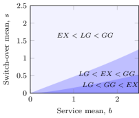
(a) $\Lambda=0.4$

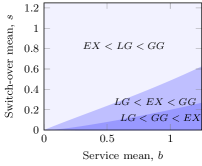
(b) $\Lambda=0.8$

Figure 5: The expected batch sojourn-time for symmetrical polling system with two queues.

6.2 Asymmetrical polling systems with multiple queues

Table 1: Parameters for three polling models.

	Model a			Model b			Model c
$Q_{i}$	1	2	3	1	2	3	1	2	3
$E\left(B_{i}\right)$	1.00	1.00	1.00	1.00	1.00	1.00	0.10	0.40	0.90
$E\left(B_{i}^{\left(2\right)}\right)$	2.00	2.00	2.00	2.00	2.00	2.00	1.00	1.00	1.00
$E\left(S_{i}\right)$	0.10	0.10	0.10	1.00	1.00	1.00	1.00	1.00	1.00
$E\left(S_{i}^{\left(2\right)}\right)$	0.02	0.02	0.02	2.00	2.00	2.00	1.00	1.00	1.00
$\boldsymbol{k}\in\mathcal{K}$	$\pi\left(1,1,0\right)=1/4$			$\pi\left(1,0,0\right)=1/3$			$\pi\left(1,1,0\right)=4/5$
	$\pi\left(3,0,1\right)=3/4$			$\pi\left(0,1,0\right)=1/3$			$\pi\left(1,0,3\right)=1/5$
				$\pi\left(0,0,1\right)=1/3$

In the previous section, we have shown that depending on the system parameters exhaustive service or locally-gated service minimizes the expected batch sojourn-time. However, it can be shown that any of the three service disciplines studied in this paper can minimize the expected batch sojourn-time. In Table 1 the parameters of three systems with $N=3$ are given. Model a has short switch-over times, Model b is a system with individual arriving customers and equal switch-over times and service times, and in Model c the last queue is the slowest and receives most of the work. Using the results of Section 3.3, Section 4.3, and Section 5.2 the expected batch sojourn-times for the three different models can be calculated. The batch sojourn-times are shown in Figure 6 for $0\leq\rho<1$. The results of Model a in Figure 6a show that locally-gated achieves the lowest expected batch sojourn-times, which is similar as in Section 6.1 when the switch-over times were short. From the results of Model b shown in Figure 6b, it can be seen that exhaustive service has the lowest expected batch sojourn-times. Here it is beneficial to serve a customer arriving to the same queue that is currently being served, since otherwise this customer has to wait a full cycle which increases the mean batch sojourn-time. Finally, Model c in Figure 6c shows that globally-gated service achieves the lowest expected batch sojourn-times, since for this policy the server will switch more often between the queues and finish service for all customers in a batch during one cycle, compared to the other disciplines.

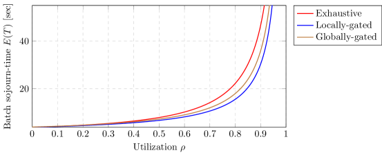
(a) Locally-gated minimizes the expected batch sojourn-time

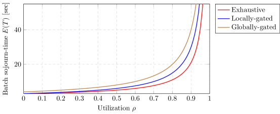
(b) Exhaustive minimizes the expected batch sojourn-time

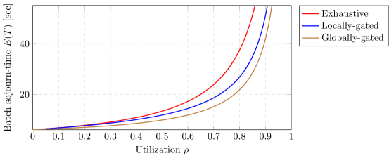
(c) Globally-gated minimizes the expected batch sojourn-time

Figure 6: The expected batch sojourn-time for various utilizations for three different systems.

7 Conclusion and further research

In this paper we analyzed the batch sojourn-time in a cyclic polling system with simultaneous batch arrivals and obtained exact expressions for the Laplace-Stieltjes transform of the steady-state batch sojourn-time distribution for the locally-gated, globally-gated, and exhaustive service disciplines. Also, we provided a more efficient way to determine the mean batch sojourn-time using the Mean Value Analysis. We compared the batch sojourn-times for the different service disciplines in several numerical examples and showed that the best performing service discipline, minimizing the batch sojourn-time, depends on system characteristics.

A further research topic would be to determine for each of the three policies, under what conditions for the system parameters, its mean batch sojourn-time is smaller than that of the other two and whether alternative service disciplines can achieve even lower batch sojourn-times. Another interesting further research topic would be to study how the customers of an arriving customer batch should be allocated over the various queues in order to minimize the batch sojourn-times.

References

- Baba, [1986] Baba, Y. (1986). On the queue with vacation time. Operations Research Letters, 5(2), 93–98.
- Boon et al., [2011] Boon, M. A. A., Van der Mei, R. D., & Winands, E. M. M. (2011). Applications of polling systems. Surveys in Operations Research and Management Science, 16(2), 67–82.
- Boon et al., [2012] Boon, M. A. A., Van der Mei, R. D., & Winands, E. M. M. (2012). Waiting times in queueing networks with a single shared server. Queueing Systems, 74(4), 403–429.
- Boxma et al., [1990] Boxma, O. J., Groenendijk, W. P., & Weststrate, J. A. (1990). A pseudoconservation law for service systems with a polling table. IEEE Transactions on Communications, 38(10), 1865–1870.
- Boxma et al., [2011] Boxma, O. J., Kella, O., & Kosinski, K. M. (2011). Queue lengths and workloads in polling systems. Operations Research Letters, 39(6), 401–405.
- Boxma et al., [1992] Boxma, O. J., Levy, H., & Yechiali, U. (1992). Cyclic reservation schemes for efficient operation of multiple-queue single-server systems. Annals of Operations Research, 35(3), 187–208.
- Chiarawongse & Srinivasan, [1991] Chiarawongse, J. & Srinivasan, M. M. (1991). On pseudo-conservation laws for the cyclic server system with compound Poisson arrivals. Operations Research Letters, 10(8), 453–459.
- Choudhury, [2002] Choudhury, G. (2002). Analysis of the queueing system with vacation times. Sankhya: The Indian Journal of Statistics, 64(1), 37–49.
- Choudhury & Whitt, [1996] Choudhury, G. L. & Whitt, W. (1996). Computing distributions and moments in polling models by numerical transform inversion. Performance Evaluation, 25(4), 267–292.
- Cohen, [1982] Cohen, J. W. (1982). The single server queue. North-Holland, Amsterdam.
- Eisenberg, [1972] Eisenberg, M. (1972). Queues with periodic service and changeover time. Operations Research, 20(2), 440–451.
- Federgruen & Katalan, [1999] Federgruen, A. & Katalan, Z. (1999). The impact of adding a make-to-order item to a make-to-stock production system. Management Science, 45(7), 980–994.
- Gong & De Koster, [2011] Gong, Y. & De Koster, M. B. M. (2011). A review on stochastic models and analysis of warehouse operations. Logistics Research, 3(4), 191–205.
- Keilson & Servi, [1988] Keilson, J. & Servi, L. D. (1988). A distributional form of Little’s Law. Operations Research Letters, 7(5), 223–227.
- Kleinrock & Levy, [1988] Kleinrock, L. & Levy, H. (1988). The Analysis of Random Polling Systems. Operations Research, 36(5), 716–732.
- Konheim et al., [1994] Konheim, A. G., Levy, H., & Srinivasan, M. M. (1994). Descendant set: an efficient approach for the analysis of polling systems. IEEE Transactions on Communications, 42(234), 1245–1253.
- Levy & Sidi, [1990] Levy, H. & Sidi, M. (1990). Polling systems: Applications, modeling, and optimization. IEEE Transactions on Communications, 38(10), 1750–1760.
- Levy & Sidi, [1991] Levy, H. & Sidi, M. (1991). Polling systems with simultaneous arrivals. IEEE Transactions on Communications, 39(6), 823–827.
- Little, [1961] Little, J. D. C. (1961). A proof of the queuing formula . Operations Research, 9(3), 383–387.
- Resing, [1993] Resing, J. A. C. (1993). Polling systems and multitype branching processes. Queueing Systems, 13(4), 409–426.
- Roodbergen & De Koster, [2001] Roodbergen, K. J. & De Koster, M. B. M. (2001). Routing methods for warehouses with multiple cross aisles. International Journal of Production Research, 39(9), 1865–1883.
- Shiozawa et al., [1990] Shiozawa, Y., Takine, T., Takahashi, Y., & Hasegawa, T. (1990). Analysis of a polling system with correlated input. Computer Networks and ISDN Systems, 20(1-5), 297–308.
- Takagi, [1986] Takagi, H. (1986). Analysis of polling systems. MIT press.
- Takagi, [2000] Takagi, H. (2000). Analysis and application of polling models. In Performance Evaluation: Origins and Directions (pp. 423–442). Springer.
- Van der Mei, [2001] Van der Mei, R. D. (2001). Polling systems with simultaneous batch arrivals. Stochastic Models, 17(3), 271–292.
- Van der Mei, [2002] Van der Mei, R. D. (2002). Waiting-time distributions in polling systems with simultaneous batch arrivals. Annals of Operations Research, 113(1-4), 155–173.
- Van der Mei et al., [2001] Van der Mei, R. D., Hariharan, R., & Reeser, P. K. (2001). Web server performance modeling. Telecommunication Systems, 16(3-4), 361–378.
- Winands et al., [2006] Winands, E. M. M., Adan, I. J. B. F., & Van Houtum, G. J. (2006). Mean value analysis for polling systems. Queueing Systems, 54(1), 35–44.
- Winands et al., [2011] Winands, E. M. M., Adan, I. J. B. F., & Van Houtum, G. J. (2011). The stochastic economic lot scheduling problem: A survey. European Journal of Operational Research, 210(1), 1–9.
- Wolff, [1982] Wolff, R. W. (1982). Poisson Arrivals See Time Averages. Operations Research, 30(2), 223–231.