Secrecy and Energy Efficiency in Massive MIMO Aided Heterogeneous C-RAN: A New Look at Interference

Abstract

In this paper, we investigate the potential benefits of the massive multiple-input multiple-output (MIMO) enabled heterogeneous cloud radio access network (C-RAN) in terms of the secrecy and energy efficiency (EE). In this network, both remote radio heads (RRHs) and massive MIMO macrocell base stations (BSs) are deployed and soft fractional frequency reuse (S-FFR) is adopted to mitigate the inter-tier interference. We first examine the physical layer security by deriving the area ergodic secrecy rate and secrecy outage probability. Our results reveal that the use of massive MIMO and C-RAN can greatly improve the secrecy performance. For C-RAN, a large number of RRHs achieves high area ergodic secrecy rate and low secrecy outage probability, due to its powerful interference management. We find that for massive MIMO aided macrocells, having more antennas and serving more users improves secrecy performance. Then we derive the EE of the heterogeneous C-RAN, illustrating that increasing the number of RRHs significantly enhances the network EE. Furthermore, it is indicated that allocating more radio resources to the RRHs can linearly increase the EE of RRH tier and improve the network EE without affecting the EE of the macrocells.

I Introduction

As a new mobile network architecture consisting of remote radio heads (RRHs) and baseband units (BBUs), cloud radio access network (C-RAN) can deal with large-scale control/data processing much more efficiently. The rationale behind this is that baseband processing is centralized and coordinated among sites in the centralized BBU pool, which reduces the capital expenditure (CAPEX) and operating expenditure (OPEX) of the networks [1]. Massive multiple-input multiple-output (MIMO) is another key technology that promises outstanding spectral efficiency (SE) and energy efficiency (EE). In massive MIMO antenna systems, base stations (BSs) are equipped with large antenna arrays to support a large number of users in the same time-frequency domain [2]. Among other emerging technologies such as device-to-device communications, full duplex radios, and millimeter wave, etc., C-RAN and massive MIMO are identified as promising 5G technologies [3, 4, 5].

Driven by its high SE and EE, C-RAN has recently received tremendous attention from both industry and academia [6, 7]. For instance, a group of single-antenna RRHs were considered to form a distributed antenna array, and two downlink transmission strategies namely best RRH selection and distributed beamforming were examined in terms of outage probability in [7]. Most recently in [8], user-centric association in a multi-tier C-RAN was proposed, in which the RRH that had the best signal-to-noise ratio (SNR) was scheduled to serve the user. Compared to [7], downlink transmission in the C-RAN with a group of multi-antenna RRHs was investigated in [9]. In the work of [9], maximal ratio transmission and transmit antenna selection were adopted at the RRHs, and the outage probability was derived by considering several transmission schemes such as RRH selection and distributed beamforming.

Heterogeneous C-RAN is a new paradigm by integrating cloud computing with heterogeneous networks (HetNets) [10, 11]. In heterogeneous C-RAN, severe inter-tier interference is coordinated for the enhancement of SE and EE. The architecture of heterogenous C-RAN with massive MIMO is envisioned as an appealing solution, since none of these techniques can solely achieve the 5G targets [4, 10]. In [10], the opportunities and challenges for heterogenous C-RAN with massive MIMO were discussed, and it was mentioned that the proper densities of the massive MIMO macrocell BSs (MBSs) and RRHs in the networks should be addressed. While the significance of heterogenous C-RAN with massive MIMO has been highlighted in the prior works [6, 10], more research efforts should be devoted to proper characterization of this combination.

Although C-RAN can effectively mitigate the inter-RRH interference by using interference management techniques such as coordinated multi-point (CoMP), the inter-tier interference between the RRHs and MBSs may be problematic in the heterogeneous C-RAN, due to the limited radio resources. Soft fractional frequency reuse (S-FFR) is viewed as an efficient inter-tier interference coordination approach. In [11], S-FFR was considered in the heterogeneous C-RAN to both mitigate the inter-tier interference and enhance the spectrum efficiency.

Recent developments have showed physical layer security as an innovative solution for safeguarding wireless networks. The rationale behind this is to exploit the randomness inherent in wireless channels such as fading or artificial noise, etc. in order to transmit information confidentially [12]. In contrast to traditional cryptographic approaches, physical layer security based techniques do not rely on computational complexity and have very good scalability [13]. The emergence of massive MIMO also introduces new opportunities for providing physical layer security, e.g., [14, 13, 15]. In particular, in [14], matched filter precoding and artificial noise generation were considered to secure downlink transmission in a multicell massive MIMO system in the presence of an eavesdropper. Subsequently in [15], passive eavesdropping and active attacks were investigated in massive MIMO systems with physical layer security, which illustrates that passive eavesdropping has little effect on the secrecy capacity for the case of considering only one single-antenna eavesdropper. While these recent contributions certainly laid a solid foundation in massive MIMO systems with physical layer security, such a research area is still far from being well understood. The research on physical layer security in the C-RAN is also in its infancy, and we believe it is a new highly rewarding candidate for physical layer security due to at least the following two crucial factors:

• Low-power RRHs are densely placed in C-RAN [1] so the distance between user and its serving RRH is short, which decreases the risk of information leakage.

• The inter-RRH interference is mitigated in the C-RAN. As such, all other RRHs can act as “friendly jammers” to confound the eavesdroppers [16, 17, 18].

Thus, massive MIMO and C-RAN offer a wealth of opportunities at the physical layer to secure communication.

Motivated by the aforementioned background, in this paper, we explore the benefits of massive MIMO aided heterogeneous C-RAN by investigating its secrecy and EE performance. We consider downlink transmission in a two-tier heterogeneous C-RAN, in which the RRHs co-exist with the massive MIMO aided macrocells. To control the inter-tier interference to an acceptable level, S-FFR is used to allocate the radio resources appropriately. Different from [11, 14, 15], in this paper, the RRHs and massive MIMO MBSs are spatially distributed under the framework of stochastic geometry. While [7, 9] considered only one single user in the network with multiple RRHs around the user coverage area and evaluated the performance from the standpoint of the user, we analyze the secrecy and EE of the entire network. In summary, our contributions are that:

• We provide a tractable analytical framework to characterize the secrecy and EE performance of heterogeneous C-RAN aided by massive MIMO. Our analysis accounts for the key features of massive MIMO and C-RAN, i.e., large antenna arrays and simultaneously serving multiple users for massive MIMO, and large numbers of RRHs and inter-RRH interference mitigation for C-RAN.

• We also study the area ergodic secrecy rate and secrecy outage probability in this network. Our results illustrate that accommodating more users by the massive MIMO empowered MBSs increases the area ergodic secrecy rate and decreases the secrecy outage probability, while it has negligible effect on the RRH’s performance. Deploying large numbers of RRHs increases the area ergodic secrecy rate and decreases the secrecy outage probability.

• In addition, our results demonstrate that the effect of S-FFR on the area ergodic secrecy rate of the network can be distinct depending on the RRH density. Moreover, the EE of the RRH tier linearly increases with their dedicated radio resources, and the network EE is improved by using more RRHs and more radio resources to be allocated to the RRHs.

II System Descriptions

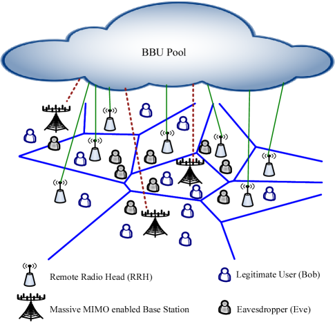
Figure 1: An illustration of two-tier heterogeneous C-RAN, where the red dash lines represent the backhual links between the macrocell base stations and BBU pool via X2/S1 interfaces, and the green solid lines represent the fronthaul links between the RRHs and BBU pool via optical fiber link.

II-A Network Model

As shown in Fig. 1, we consider the downlink of a two-tier heterogeneous C-RAN, where the BBU pool in the cloud is established to coordinate the entire network. Massive MIMO enabled MBSs of the first tier, as high power nodes (HPNs), are connected with the BBU pool via backhaul link, while the RRHs of the second tier, as low power nodes (LPNs), are connected with the BBU pool via fronthaul link (optical fibre link). In this model, we have eavesdroppers (Eves) passively intercepting the secrecy messages without any active attacks. The locations of Eves are modeled as a homogeneous Poisson point process (HPPP) $\Phi_{e}$ with density $\lambda_{e}$. On the other hand, the locations of MBSs are modeled as an independent HPPP $\Phi_{\mathrm{M}}$ with density $\lambda_{\mathrm{M}}$, and we model the locations of RRHs by an independent HPPP $\Phi_{\mathrm{R}}$ with density $\lambda_{\mathrm{R}}$.

Equipped with $N_{\mathrm{M}}$ antennas, each MBS uses zero-forcing beamforming (ZFBF) to communicate with $S$ single-antenna users over the same resource block (RB) ($N_{\mathrm{M}}\gg S\geq 1$) using equal power assignment. The ZFBF matrix at a MBS is ${\bf{W}}{\rm{=}}{\bf{G}}{\left({{{\bf{G}}^{H}}{\bf{G}}}\right)^{-1}}$ with the channel matrix $\bf{G}$ [20], where $(\cdot)^{H}$ denotes the Hermitian transpose. Each RRH is equipped with a single-antenna and serves a single-antenna user over one RB. All channels are assumed to undergo independent identically distributed (i.i.d.) quasi-static Rayleigh block fading. Further, each user is assumed to be connected with its nearest BS such that the Euclidean plane is divided into Poisson-Voronoi cells.

We consider the adoption of S-FFR for inter-tier interference mitigation and assume that there are a total of $K$ RBs, the number of RBs allocated to RRHs is $\alpha K$, and the number of RBs shared by RRHs and MBSs is $\left(1-\alpha\right)K$, in which $\alpha$ denotes the S-FFR factor, with $\left(0\leq\alpha\leq 1\right)$. Since inter-RRH interference can be efficiently mitigated via cooperation among RRHs, same radio resources can be shared among the RRHs in the C-RAN [11]. For RRH transmission over the $k$-th RB allocated to RRHs, the receive signal-to-interference-plus-noise ratio (SINR) at a typical user can be expressed as

$$\gamma_{\mathrm{R},k} =\frac{P_{\mathrm{R}}}{B_{o}N_{o}}h_{\mathrm{R},k}\beta\left|{{X_{{o},\mathrm{R}}}}\right|^{-\eta_{\mathrm{R}}},\quad k=1,\dots,\alpha K$$ (1)

where $P_{\mathrm{R}}$ is the RRH transmit power allocated to each RB, $B_{o}$ is the bandwidth per RB, $h_{\mathrm{R},k}\sim\rm{exp}(1)$ is the small-scale fading channel power gain, $\beta$ is a frequency dependent constant value, which is typically set as ${(\frac{{\text{c}}}{{4\pi{f_{c}}}})^{2}}$ with $c=3\times 10^{8}\rm m/s$ and the carrier frequency $f_{c}$, $\eta_{\mathrm{R}}$ is the pathloss exponent, $\left|{{X_{{o},\mathrm{R}}}}\right|$ denotes the distance between the typical user and its typical serving RRH, and $N_{o}$ is the power spectrum density of the noise and the weak inter-RRH interference. For RRH transmission over the $\nu$-th RB shared by the RRHs and MBSs, the receive SINR at a typical user is written as

$$\gamma_{\mathrm{R},\nu} =\frac{P_{\mathrm{R}}h_{\mathrm{R},\nu}\beta\left|{{X_{{o},\mathrm{R}}}}\right|^{-\eta_{\mathrm{R}}}}{I_{\mathrm{M},\nu}+B_{o}N_{o}},\quad\nu=1,\dots,\left(1-\alpha\right)K$$ (2)

where $h_{\mathrm{R},\nu}\sim\rm{exp}(1)$ is the small-scale fading channel power gain, $I_{\mathrm{M},\nu}$ is the inter-tier interference from the MBSs, which is given by

$$I_{\mathrm{M},\nu}=\sum\limits_{\ell\in{\Phi_{\mathrm{M}}}}{\frac{P_{\mathrm{M}}}{S}{h_{\ell,\nu}}\beta\left|{{X_{\ell,\mathrm{M}}}}\right|^{-\eta_{\mathrm{M}}}},$$ (3)

where $P_{\mathrm{M}}$ is the MBS transmit power of each RB, $h_{\ell,\nu}\sim\Gamma\left(S,1\right)$ is the small-scale fading interfering channel power gain, $\left|{{X_{\ell,\mathrm{M}}}}\right|$ is the distance between the interfering MBS $\ell\in{\Phi_{\mathrm{M}}}$ and the typical user, and $\eta_{\mathrm{M}}$ is the pathloss exponent.

We consider the non-colluding eavesdropping scenario where the most malicious Eve i.e., the one with the largest SINR of the received signal, dominates the secrecy rate [12]. Thus, for RRH transmissions over the $k$-th and $\nu$-th RB, the receive SINRs at the most malicious Eve ${e^{*}}$ are given by

$$\gamma_{\mathrm{R},k}^{e^{*}}=\mathop{\max}\limits_{e\in\Phi_{e}}\left\{\frac{{{P_{\mathrm{R}}}h_{\mathrm{R}{\rm{,}}k}^{e}\beta{{\left|{X_{o{\rm{,}}\mathrm{R}}^{e}}\right|}^{-{\eta_{\mathrm{R}}}}}}}{{I_{\mathrm{R},k}^{e}+{B_{o}}{N_{e}}}}\right\},$$ (4)

and

$$\gamma_{\mathrm{R},\nu}^{e^{*}}=\mathop{\max}\limits_{e\in\Phi_{e}}\left\{\frac{{{P_{\mathrm{R}}}h_{\mathrm{R}{\rm{,}}\nu}^{e}\beta{{\left|{X_{o{\rm{,}}\mathrm{R}}^{e}}\right|}^{-{\eta_{\mathrm{R}}}}}}}{{I_{\mathrm{R},\nu}^{e}+I_{\mathrm{M},\nu}^{e}+{B_{o}}{N_{e}}}}\right\},$$ (5)

respectively, where $h_{\mathrm{R}{\rm{,}}i}^{e}(i\in\left\{k,\nu\right\})\sim\rm{exp}(1)$ and $\left|{X_{o{\rm{,}}\mathrm{R}}^{e}}\right|$ are the small-scale fading eavesdropping channel power gain and the distance between the typical serving RRH and the Eve $e\in\Phi_{e}$, respectively, $N_{e}$ is the noise power spectrum density, $I_{\mathrm{R},i}^{e}$ and $I_{\mathrm{M},\nu}^{e}$ are the interference from the RRHs and MBSs, which are found as

$$\left\{\begin{aligned} I_{\mathrm{R},i}^{e}&=\sum\limits_{j\in{\Phi_{\mathrm{R}}}/{o}}{{P_{\mathrm{R}}}{h_{j,i}^{e}}\beta\left|{{X_{j,\mathrm{R}}^{e}}}\right|^{-\eta_{\mathrm{R}}}},\\ I_{\mathrm{M},\nu}^{e}&=\sum\limits_{\ell\in{\Phi_{\mathrm{M}}}}{\frac{P_{\mathrm{M}}}{S}{h_{\ell,\nu}^{e}}\beta\left|{{X_{\ell,\mathrm{M}}^{e}}}\right|^{-\eta_{\mathrm{M}}}},\end{aligned}\right.$$ (6)

where ${h_{j,i}^{e}}\sim\rm{exp}(1)$ and $\left|{{X_{j,\mathrm{R}}^{e}}}\right|$ are the small-scale fading interfering channel power gain and the distance between the RRH $j\in{\Phi_{\mathrm{R}}}/{o}$ (except the typical serving RRH) and the Eve, respectively, ${h_{\ell,\nu}^{e}}\sim\Gamma\left(S,1\right)$ [20] and $\left|{{X_{\ell,\mathrm{M}}^{e}}}\right|$ are the small-scale fading interfering channel power gain and the distance between the MBS $\ell\in{\Phi_{\mathrm{M}}}$ and the Eve, respectively.

Due to the limited backhaul capacity, the inter-MBS interference is assumed to be not mitigated. Thus, for MBS transmission over the $\nu$-th RB shared by RRHs and MBSs, the receive SINR at a typical user is written as

$$\gamma_{\mathrm{M},\nu}=\frac{\frac{P_{\mathrm{M}}}{S}g_{\mathrm{M},\nu}\beta\left|{{X_{{o},\mathrm{M}}}}\right|^{-\eta_{\mathrm{M}}}}{J_{\mathrm{M},\nu}+J_{\mathrm{R},\nu}+B_{o}N_{1}},$$ (7)

where $g_{\mathrm{M},\nu}\sim\Gamma\left(N_{\mathrm{M}}-S+1,1\right)$ is the small-scale fading channel power gain, $\left|{{X_{{o},\mathrm{M}}}}\right|$ is the distance between the typical user and its typical serving MBS, $N_{1}$ is the power spectrum density of the noise. In (7), $J_{\mathrm{M},\nu}$ and $J_{\mathrm{R},\nu}$ are the interference from MBSs and RRHs, which are given by

$$\left\{\begin{aligned} J_{\mathrm{M},\nu}&=\sum\limits_{\ell\in{\Phi_{\mathrm{M}}}/{o}}{\frac{P_{\mathrm{M}}}{S}{g_{\ell,\nu}}\beta\left|{{X_{\ell,\mathrm{M}}}}\right|^{-\eta_{\mathrm{M}}}},\\ J_{\mathrm{R},\nu}&=\sum\limits_{j\in{\Phi_{\mathrm{R}}}}{{P_{\mathrm{R}}}{g_{j,\nu}}\beta\left|{{X_{j,\mathrm{R}}}}\right|^{-\eta_{\mathrm{R}}}},\end{aligned}\right.$$ (8)

where $g_{\ell,\nu}\sim\Gamma\left(S,1\right)$ and $\left|{{X_{\ell,\mathrm{M}}}}\right|$ are the small-scale fading interfering channel power gain and the distance between the interfering MBS $\ell\in{\Phi_{\mathrm{M}}}/{o}$ (except the typical serving MBS) and the typical user, respectively, $g_{j,\nu}\sim\exp\left(1\right)$ and $\left|{{X_{j,\mathrm{R}}}}\right|$ are the small-scale interfering channel power gain and the distance between the interfering RBS $j\in{\Phi_{\mathrm{R}}}$ and the typical user, respectively.

Similar to (5), for MBS transmission, the receive SINR $\gamma_{\mathrm{M},\nu}^{e^{*}}$ at the most malicious Eve ${e^{*}}$ is given by

$$\gamma_{\mathrm{M},\nu}^{e^{*}}=\mathop{\max}\limits_{e\in\Phi_{e}}\left\{\frac{\frac{P_{\mathrm{M}}}{S}g_{\mathrm{M},\nu}^{e}\beta\left|{{X_{{o},\mathrm{M}}^{e}}}\right|^{-\eta_{\mathrm{M}}}}{J_{\mathrm{M},\nu}^{e}+J_{\mathrm{R},\nu}^{e}+B_{o}N_{e}}\right\},$$ (9)

where $g_{\mathrm{M},\nu}^{e}\sim\exp\left(1\right)$ and $\left|{{X_{{o},\mathrm{M}}^{e}}}\right|$ are the small-scale fading channel power gain and distance between the typical serving MBS and the Eve, respectively. In particular, we consider the worst-case scenario that Eves are capable of mitigating the intra-cell interference [19]. In (9), $J_{\mathrm{M},\nu}^{e}$ and $J_{\mathrm{R},\nu}^{e}$ are the interference from the MBSs and RRHs, respectively, given by

$$\left\{\begin{aligned} J_{\mathrm{M},\nu}^{e}&=\sum\limits_{\ell\in{\Phi_{\mathrm{M}}}/{o}}{\frac{P_{\mathrm{M}}}{S}{g_{\ell,\nu}^{e}}\beta\left|{{X_{\ell,\mathrm{M}}^{e}}}\right|^{-\eta_{\mathrm{M}}}},\\ J_{\mathrm{R},\nu}^{e}&=\sum\limits_{j\in{\Phi_{\mathrm{R}}}}{{P_{\mathrm{R}}}{g_{j,\nu}^{e}}\beta\left|{{X_{j,\mathrm{R}}^{e}}}\right|^{-\eta_{\mathrm{R}}}},\end{aligned}\right.$$ (10)

where $g_{\ell,\nu}^{e}\sim\Gamma\left(S,1\right)$ and $\left|{{X_{\ell,\mathrm{M}}^{e}}}\right|$ are the small-scale fading interfering channel power gain and the distance between the interfering MBS $\ell\in{\Phi_{\mathrm{M}}}/{o}$ (except the typical serving MBS) and Eve, respectively, and ${g_{j,\nu}^{e}}\sim\exp\left(1\right)$ and $\left|{{X_{j,\mathrm{R}}^{e}}}\right|$ are the small-scale fading interfering channel power gain and the distance between the interfering RRH $j\in{\Phi_{\mathrm{R}}}$ and Eve, respectively.

II-B Power Consumption Model

The total power consumption at each RRH is given by

$$P_{\mathrm{R}}^{total}=K\frac{{{P_{\mathrm{R}}}}}{\varepsilon_{\mathrm{R}}}+P_{\mathrm{R}}^{0}+P_{\mathrm{fh}},$$ (11)

in which $\varepsilon_{\mathrm{R}}$ is the efficiency of the power amplifier, $P_{\mathrm{R}}^{0}$ is the static hardware power consumption of the RRH, and $P_{\mathrm{fh}}$ denotes the power consumption of the fronthaul link.

We employ a general massive MIMO power consumption model proposed in [22], which can clearly specify how the power scales with the number of antennas and active users in each macrocell. Thus, the total power consumption at each MBS is found as

$$P_{\mathrm{M}}^{total}= {\left(1-\alpha\right)K}\Big{(}\frac{{{P_{\mathrm{M}}}}}{\varepsilon_{\mathrm{M}}}+\sum\limits_{\rho=1}^{3}\big{(}{\left(S\right)^{\rho}}{\Lambda_{\rho,0}}$$

$$\;\;\;\;~{}~{}~{}+{\left(S\right)^{\left(\rho-1\right)}}N_{\mathrm{M}}{\Lambda_{\rho,1}}\big{)}\Big{)}+P_{\mathrm{M}}^{0}+P_{\mathrm{bh}},$$ (12)

where $\varepsilon_{\mathrm{M}}\left(0<\varepsilon_{\mathrm{M}}\leq 1\right)$ is the efficiency of the power amplifier, the parameters $\Lambda_{\rho,0}$ and $\Lambda_{\rho,1}$ depend on the transceiver chains, coding and decoding, precoding, etc., which are detailed in Section V, $P_{\mathrm{M}}^{0}$ is the MBS’s static hardware power consumption, and $P_{\mathrm{bh}}$ is the power consumption of the backhaul link.

III Secrecy Performance Analysis

In this section, the effects of massive MIMO and C-RAN on the secrecy performance are studied in terms of both the area ergodic secrecy rate and secrecy outage probability.

Secrecy outage probability captures the probability of both reliability and secrecy for one transmission.

III-A Area Ergodic Secrecy Rate

Area ergodic secrecy rate represents the secrecy capacity limitation of the network, which allows us to investigate the impacts of different densities of RRHs and massive MIMO macrocells on the network secrecy performance. We first study the ergodic capacity of the channel between the typical RRH and its served user, which is given as follows.

Theorem 1.

When using the $k$-th RB allocated to the RRHs, the ergodic capacity $\bar{C}_{\mathrm{R},k}$ of the channel between the typical RRH and its served user is derived as (13) (see top of next page). When using the $\nu$-th RB shared by the RRHs and MBSs, the ergodic capacity $\bar{C}_{\mathrm{R},\nu}$ of the channel between the typical RRH and its served user is derived as (14), where $\mathrm{B}_{\left(\cdot\right)}\left[\cdot,\cdot\right]$ is the incomplete beta function [21, (8.391)].

Proof.

A detailed proof is provided in Appendix A. ∎

$$\bar{C}_{\mathrm{R},k}=\frac{2\pi}{{\ln 2}}\left({{\lambda_{\mathrm{R}}}+{\lambda_{\mathrm{M}}}}\right)\int_{0}^{\infty}{{e^{\frac{{{B_{o}}{N_{o}}}}{{{P_{\rm{R}}}\beta}}{x^{{\eta_{\rm{R}}}}}}}\Gamma\left({0,\frac{{{B_{o}}{N_{o}}}}{{{P_{\rm{R}}}\beta}}{x^{{\eta_{\rm{R}}}}}}\right)x{e^{-\pi\left({{\lambda_{\mathrm{R}}}+{\lambda_{\mathrm{M}}}}\right){x^{2}}}}dx},$$ (13)

$$\bar{C}_{\mathrm{R},\nu}=\frac{2\pi}{{\ln 2}}\left({{\lambda_{\mathrm{R}}}+{\lambda_{\mathrm{M}}}}\right)\int_{0}^{\infty}{\left[{\int_{0}^{\infty}{\frac{{\bar{F}}_{{\gamma_{\mathrm{R},\nu}}\mid\left\{\left|{{X_{o,{\rm{R}}}}}\right|=x\right\}}\left(\gamma\right)}{{1+\gamma}}d\gamma}}\right]x{e^{-\pi\left({{\lambda_{\mathrm{R}}}+{\lambda_{\mathrm{M}}}}\right){x^{2}}}}dx},$$ (14)

with

$${\bar{F}}_{{\gamma_{\mathrm{R},\nu}}\mid\left\{\left|{{X_{o,{\rm{R}}}}}\right|=x\right\}}\left(\gamma\right)={e^{-\frac{{{B_{o}}{N_{o}}}}{{{P_{\rm{R}}}\beta}}{x^{{\eta_{\rm{R}}}}}\gamma}}\times$$

$$\exp\bigg{\{}-{\lambda_{\mathrm{M}}}2\pi\sum\limits_{\mu=1}^{S}{{S\choose\mu}{{\left({\frac{{x^{{\eta_{\rm{R}}}}}\gamma{{P_{\mathrm{M}}}}}{{P_{\rm{R}}S}}}\right)}^{\mu}}}\frac{{\left({\frac{{x^{{\eta_{\rm{R}}}}}\gamma{{P_{\mathrm{M}}}}}{{P_{\rm{R}}S}}}\right)^{-\mu+\frac{2}{{{\eta_{\mathrm{M}}}}}}}}{{{\eta_{\mathrm{M}}}}}{B_{\left(-{\frac{{x^{{\eta_{\rm{R}}}-\eta_{\mathrm{M}}}}\gamma{{P_{\mathrm{M}}}}}{{P_{\rm{R}}S}}}\right)}}\left[{\mu-\frac{2}{{{\eta_{\mathrm{M}}}}},1-S}\right]\bigg{\}}$$ (15)

$$\bar{C}_{\mathrm{R},k}^{e^{*}}=\frac{1}{{\ln 2}}\int_{0}^{\infty}\frac{1-F_{\gamma_{\mathrm{R},k}^{e^{*}}}\left(x\right)}{1+x}dx,$$ (16)

with

$$F_{\gamma_{\mathrm{R},k}^{e^{*}}}\left(x\right)=\exp\bigg{\{}-2\pi{\lambda_{e}}\int_{0}^{\infty}\exp\Big{[}-\frac{{r}^{{\eta_{\mathrm{R}}}}x}{{P_{\mathrm{R}}}\beta}{B_{o}}{N_{e}}-\lambda_{\mathrm{R}}\pi\Gamma\left(1+\frac{2}{\eta_{\mathrm{R}}}\right)\Gamma\left(1-\frac{2}{\eta_{\mathrm{R}}}\right)\big{(}{{r}^{{\eta_{\mathrm{R}}}}x}\big{)}^{\frac{2}{\eta_{\mathrm{R}}}}\Big{]}rdr\bigg{\}}$$ (17)

$$\bar{C}_{\mathrm{R},\nu}^{e^{*}}=\frac{1}{{\ln 2}}\int_{0}^{\infty}\frac{1-F_{\gamma_{\mathrm{R},\nu}^{e^{*}}}\left(x\right)}{1+x}dx,$$ (18)

with

$$F_{\gamma_{\mathrm{R},\nu}^{e^{*}}}\left(x\right)= \exp\bigg{\{}-2\pi{\lambda_{e}}\int_{0}^{\infty}\exp\Big{[}-\frac{{r}^{{\eta_{\mathrm{R}}}}x}{{P_{\mathrm{R}}}\beta}{B_{o}}{N_{e}}-\lambda_{\mathrm{R}}\pi\Gamma\left(1+\frac{2}{\eta_{\mathrm{R}}}\right)\Gamma\left(1-\frac{2}{\eta_{\mathrm{R}}}\right)\big{(}{{r}^{{\eta_{\mathrm{R}}}}x}\big{)}^{\frac{2}{\eta_{\mathrm{R}}}}$$

$$-2\pi\lambda_{\mathrm{M}}\sum\limits_{\mu=1}^{S}{S\choose\mu}\left(\frac{{r}^{{\eta_{\mathrm{R}}}}xP_{\mathrm{M}}}{P_{\mathrm{R}}S}\right)^{\frac{2}{\eta_{\mathrm{M}}}}\frac{\Gamma\left(\mu-\frac{2}{\eta_{\mathrm{M}}}\right)\Gamma\left(-\mu+\frac{2}{\eta_{\mathrm{M}}}+S\right)}{\eta_{\mathrm{M}}\Gamma\left(S\right)}\Big{]}rdr\bigg{\}}$$ (19)

We next derive the ergodic capacity of the channel between the most malicious eavesdropper and the typical RRH, which is given as follows:

Theorem 2.

For RRH transmissions over the $k$-th RB and $\nu$-th RB, the ergodic capacity $\bar{C}_{\mathrm{R},k}^{e^{*}}$ and $\bar{C}_{\mathrm{R},\nu}^{e^{*}}$ of the most malicious eavesdropper’s channel are derived as (16) and (18), respectively, in the next page.

Proof.

A detailed proof is provided in Appendix B. ∎

Based on Theorem 1 and Theorem 2 , using Jensen’s inequality that $\mathbb{E}\left\{{\max\left({X{\rm{,}}Y}\right)}\right\}\geq\max\left({\mathbb{E}\left\{x\right\}{\rm{,}}\mathbb{E}\left\{Y\right\}}\right)$, the ergodic secrecy rate for the typical RRH transmission over the $k$-th RB is lower bounded as [23, 14]

$$R_{\mathrm{R},k}^{\mathrm{s}}=\left[\bar{C}_{\mathrm{R},k}-\bar{C}_{\mathrm{R},k}^{e^{*}}\right]^{+},$$ (20)

where $[x]^{+}=\max\left\{x,0\right\}$.

Likewise, the ergodic secrecy rate for the typical RRH transmission over the $\nu$-th RB is lower bounded as

$$R_{\mathrm{R},\nu}^{\mathrm{s}}=\left[\bar{C}_{\mathrm{R},\nu}-\bar{C}_{\mathrm{R},\nu}^{e^{*}}\right]^{+}.$$ (21)

Remark 2: From the results in Theorem 1, Theorem 2, (20) and (21), we realize that the ergodic secrecy rate for RRH transmission increases with the density of RRHs, which can be explained by the facts that: 1) When deploying more RRHs in the same area, the distance between the legitimate user and its associated RRH is shorter, which decreases the pathloss; and 2) more interference from RRHs is present at the eavesdroppers, which degrades the eavesdropping channel.

The area ergodic secrecy rate (in bits/s/m²) of the RRH tier in the heterogeneous C-RAN is calculated as

$$R_{\mathrm{R}}^{\mathrm{s}}=\lambda_{\mathrm{R}}\left(\alpha KB_{o}R_{\mathrm{R},k}^{\mathrm{s}}+\left(1-\alpha\right)KB_{o}R_{\mathrm{R},\nu}^{\mathrm{s}}\right).$$ (22)

For MBS transmission, we have a tractable lower bound expression for the ergodic capacity of the channel between the typical MBS and its serving user as stated in the following theorem.

Theorem 3.

For MBS transmission over the $\nu$-th RB, the ergodic capacity of the channel between the typical MBS and its served user is lower bounded in closed-form as

$$\vspace{-0.5 cm}\bar{C}_{\mathrm{M},\nu}^{\mathrm{L}}=\log_{2}\Bigg{(}1+\exp\bigg{(}\ln\left({\frac{{{P_{\rm{M}}}}}{S}\beta}\right)+\psi\left(N_{\mathrm{M}}-S+1\right)-\frac{\eta_{\rm{M}}}{2}$$

$$\vspace{-0.5 cm}\left(\psi\left(1\right)-\ln\left({\pi\left({{\lambda_{\rm{R}}}+{\lambda_{\rm{M}}}}\right)}\right)\right)-\ln\Big{(}{\frac{{{P_{\mathrm{M}}}\beta 2\pi{\lambda_{\mathrm{M}}}}\Gamma\left(2-\frac{\eta_{\mathrm{M}}}{2}\right)}{{\left({\eta_{\mathrm{M}}}-2\right)\left(\pi\lambda_{\mathrm{M}}+\pi\lambda_{\mathrm{R}}\right)^{1-\frac{\eta_{\mathrm{M}}}{2}}}}}$$

$$+{\frac{{{P_{\mathrm{R}}}\beta 2\pi{\lambda_{\mathrm{R}}}}\Gamma\left(2-\frac{\eta_{\mathrm{R}}}{2}\right)}{{\left({\eta_{\mathrm{R}}}-2\right)\left(\pi\lambda_{\mathrm{M}}+\pi\lambda_{\mathrm{R}}\right)^{1-\frac{\eta_{\mathrm{R}}}{2}}}}}+B_{o}N_{1}\Big{)}\bigg{)}\Bigg{)},$$ (23)

where $\psi\left(\cdot\right)$ is the digamma function [24]. For very large $N_{\mathrm{M}}$, $\psi\left(N_{\mathrm{M}}-S+1\right)\approx\ln\left(N_{\mathrm{M}}-S+1\right)$ [25].

Proof.

A detailed proof is provided in Appendix C. ∎

For MBS transmission over the $\nu$-th RB, the ergodic capacity $\bar{C}_{\mathrm{M},\nu}^{e^{*}}$ of the most malicious eavesdropper’s channel is derived as

$$\bar{C}_{\mathrm{M},\nu}^{e^{*}} =\mathbb{E}\left\{\log_{2}\left(1+\gamma_{\mathrm{M},\nu}^{e^{*}}\right)\right\}$$

$$=\frac{1}{{\ln 2}}\int_{0}^{\infty}\frac{1-F_{\gamma_{\mathrm{M},\nu}^{e^{*}}}\left(x\right)}{1+x}dx,$$ (24)

where $F_{\gamma_{\mathrm{M},\nu}^{e^{*}}}\left(x\right)$ is given by (III-A) in the next page, which can be easily obtained by following the proof of Theorem 2.

$$F_{\gamma_{\mathrm{M},\nu}^{e^{*}}}\left(x\right)=\exp\bigg{\{}-2\pi{\lambda_{e}}\int_{0}^{\infty}\exp\bigg{[}-\frac{S{r}^{{\eta_{\mathrm{M}}}}x}{{P_{\mathrm{M}}}\beta}{B_{0}}{N_{1}}-\lambda_{\mathrm{R}}\pi\left(P_{\mathrm{R}}\beta\right)^{\frac{2}{\eta_{\mathrm{R}}}}\Gamma\left(1+\frac{2}{\eta_{\mathrm{R}}}\right)\Gamma\left(1-\frac{2}{\eta_{\mathrm{R}}}\right)$$

$$\left(\frac{S{r}^{{\eta_{\mathrm{M}}}}x}{{P_{\mathrm{M}}}\beta}\right)^{\frac{2}{\eta_{\mathrm{R}}}}-2\pi\lambda_{\mathrm{M}}\sum\limits_{\mu=1}^{S}{S\choose\mu}\left({{r}^{{\eta_{\mathrm{M}}}}x}\right)^{\frac{2}{\eta_{\mathrm{M}}}}\frac{\Gamma\left(\mu-\frac{2}{\eta_{\mathrm{M}}}\right)\Gamma\left(-\mu+\frac{2}{\eta_{\mathrm{M}}}+S\right)}{\eta_{\mathrm{M}}\Gamma\left(S\right)}\Bigg{]}rdr\Bigg{\}}$$ (25)

Based on Theorem 3 and (III-A), the ergodic secrecy rate for the typical MBS transmission over the $\nu$-th RB is lower bounded as

$$R_{\mathrm{M},\nu}^{\mathrm{s}}=\left[\bar{C}_{\mathrm{M},\nu}^{\mathrm{L}}-\bar{C}_{\mathrm{M},\nu}^{e^{*}}\right]^{+}.$$ (26)

Remark 3: From the results in (3), (III-A), and (26), we establish that the ergodic secrecy rate is improved by increasing the number of MBS antennas, due to the fact that only the served legitimate users can obtain the large array gains.

The area ergodic secrecy rate (in bits/s/m²) of the MBS tier in the heterogeneous C-RAN is calculated as

$$R_{\mathrm{M}}^{\mathrm{s}}=\lambda_{\mathrm{M}}\left(1-\alpha\right)KB_{o}SR_{\mathrm{M},\nu}^{\mathrm{s}}.$$ (27)

III-B Secrecy Outage Probability

In the above, we have studied the secrecy capacity in the massive MIMO aided heterogeneous C-RAN. Since Eves only intercept the secrecy massages passively without any transmissions, the channel state information (CSI) of the eavesdropping channels cannot be obtained by the BSs or legitimate users. In this circumstance, the BSs set the transmission rate $R$ consisting of the secrecy codewords and non-secrecy codewords, and a constant rate of the secrecy codewords $R_{\mathrm{s}}\left(R_{\mathrm{s}}\leq R\right)$. Secrecy outage is declared when the targeted secrecy rate $R_{\mathrm{s}}$ cannot be guaranteed.

III-B1 Delay-Limited Mode

In the delay-limited mode, a rate $R$ is set under certain connection outage constraint. For RRH transmission over the $k$-th RB allocated to the RRHs, given a distance $\left|{{X_{{0},\mathrm{R}}}}\right|=d_{0}$ between a typical RRH and its serving user, the connection outage probability is given by

$$P_{\mathrm{R},k}^{\mathrm{co}}\left(R\right) =\Pr\left(\log_{2}\left(1+\gamma_{\mathrm{R},k}\right)<R\right)$$

$$=1-\exp\left(-\frac{B_{o}N_{o}}{P_{\mathrm{R}}\beta}d_{o}^{\eta_{\mathrm{R}}}\left(2^{R}-1\right)\right).$$ (28)

For RRH transmission over the $\nu$-th RB shared by RRHs and MBSs, the connection outage probability is

$$P_{\mathrm{R},\nu}^{\mathrm{co}}\left(R\right) =\Pr\left(\log_{2}\left(1+\gamma_{\mathrm{R},\nu}\right)<R\right)$$

$$=1-{\bar{F}}_{{\gamma_{\mathrm{R},\nu}}\mid\left\{\left|{{X_{o,{\rm{R}}}}}\right|=d_{o}\right\}}\left(2^{R}-1\right),$$ (29)

where ${\bar{F}}_{{\gamma_{\mathrm{R},\nu}}\mid\left\{\left|{{X_{o,{\rm{R}}}}}\right|=x\right\}}\left(\cdot\right)$ is given by (III-A).

Remark 4: From (III-B1) and (III-B1), we see that when a typical RRH transmits information to its served user, deploying more RRHs in its surrounding area has no effect on the quality of connectivity, since the inter-RRH interference is mitigated.

Corollary 1.

Given a distance $\left|{{X_{{o},\mathrm{R}}}}\right|=d_{o}$ and the connection outage probability threshold $\sigma$, the typical RRH transmission rate over the $k$-th RB allocated to RRHs is given by

$$R={\log_{2}}\left({1-\frac{{{P_{\rm{R}}}\beta}}{{{B_{o}}{N_{o}}{d_{o}^{{\eta_{\rm{R}}}}}}}\ln\left({1-\sigma}\right)}\right),$$ (30)

and the typical RRH transmission rate over the $\nu$-th RB shared by RRHs and MBSs satisfies

$$R\geq\log_{2}\left(1+\frac{{{P_{\mathrm{R}}}S}}{{{P_{\mathrm{M}}}{d_{o}^{{\eta_{R}}}}}}\Delta_{1}^{\frac{{{\eta_{\mathrm{M}}}}}{2}}\right),$$ (31)

with

$$\Delta_{1}={-\frac{{{\eta_{\mathrm{M}}}\Gamma\left(S\right)\ln\left({1-\sigma}\right)}}{{2\pi{\lambda_{\mathrm{M}}}\sum\limits_{\mu=1}^{S}{{S\choose\mu}\Gamma\left({\mu-\frac{2}{{{\eta_{\mathrm{M}}}}}}\right)\Gamma\left({-\mu+\frac{2}{{{\eta_{\mathrm{M}}}}}+S}\right)}}}}.$$ (32)

Proof.

A detailed proof is provided in Appendix D. ∎

Similar to (III-B1), given a distance $\left|{{X_{{o},\mathrm{M}}}}\right|=d_{o}$ between a typical MBS and its served user, we obtain the connection outage probability of MBS transmission as

$$\mathrm{P}_{\mathrm{M},\nu}^{\mathrm{co}}\left(R\right)=1-{\bar{F}}_{{\gamma_{\mathrm{M},\nu}}\mid\left\{\left|{{X_{o,{\rm{M}}}}}\right|=d_{o}\right\}}\left(2^{R}-1\right),$$ (33)

where ${\bar{F}}_{{\gamma_{\mathrm{M},\nu}}\mid\left\{\left|{{X_{o,{\rm{M}}}}}\right|=d_{o}\right\}}\left(\cdot\right)$ is the complementary cumulative distribution function (CCDF) of the receive SINR $\gamma_{\mathrm{M},\nu}$ at the MBS. However, the exact expression for ${\bar{F}}_{{\gamma_{\mathrm{M},\nu}}\mid\left\{\left|{{X_{o,{\rm{M}}}}}\right|=d_{o}\right\}}\left(\cdot\right)$ involves higher order derivatives of laplace transform using $\mathrm{Fa\grave{a}}$ di Bruno’s formula [26], which becomes inefficient for large number of MBS antennas. By the law of large numbers, i.e., $g_{\mathrm{M},\nu}\approx N_{\mathrm{M}}-S+1$ as $N_{\mathrm{M}}$ is large, and employing Gil-Pelaez theorem [27], we have

$${\bar{F}}_{{\gamma_{\mathrm{M},\nu}}\mid\left\{\left|{{X_{o,{\rm{M}}}}}\right|=d_{o}\right\}}\left(\gamma\right)=\Pr\Big{(}\frac{\frac{P_{\mathrm{M}}}{S}\left(N_{\mathrm{M}}-S+1\right)\beta d_{o}^{-\eta_{\mathrm{M}}}}{J_{\mathrm{M},\nu}+J_{\mathrm{R},\nu}+B_{o}N_{1}}>\gamma\Big{)}$$

$$=\Pr\Big{(}J_{\mathrm{M},\nu}+J_{\mathrm{R},\nu}<\Big{(}\frac{P_{\mathrm{M}}}{S\gamma}\left(N_{\mathrm{M}}-S+1\right)\beta d_{o}^{-\eta_{\mathrm{M}}}-B_{o}N_{1}\Big{)}\Big{)}$$

$$=\frac{1}{2}-\frac{1}{\pi}\int_{0}^{\infty}\frac{\mathrm{Im}\big{[}e^{-jw\big{(}\frac{P_{\mathrm{M}}\beta}{Sd_{o}^{\eta_{\mathrm{M}}}\gamma}\left(N_{\mathrm{M}}-S+1\right)-B_{o}N_{1}\big{)}}\varphi^{*}\left(w\right)\big{]}}{w}dw,$$ (34)

where $j=\sqrt{-1}$, $\varphi\left(w\right)$ is the conjugate of the characteristic function given by (III-B1) (See top of this page), which can be easily obtained by following the similar approach in Appendix A. In (III-B1), ${}_{2}{F_{1}}\left[\cdot,\cdot;\cdot;\cdot\right]$ is the Gauss hypergeometric function [21, (9.142)].

$$\varphi\left(w\right)=\exp\bigg{(}-2\pi{\lambda_{\mathrm{R}}}\frac{jwP_{\mathrm{R}}\beta d_{o}^{2-\eta_{\mathrm{R}}}}{\eta_{\mathrm{R}}-2}{}_{2}{F_{1}}\left[1,{\frac{{\eta_{\mathrm{R}}-2}}{{{\eta_{\mathrm{R}}}}};2-\frac{2}{{{\eta_{\mathrm{R}}}}};-jwP_{\mathrm{R}}\beta{d_{o}^{-{\eta_{\mathrm{R}}}}}}\right]-{\lambda_{\mathrm{M}}}2\pi\sum\limits_{\mu=1}^{S}$$

$${{S\choose\mu}{{\left({jw\frac{{{P_{\mathrm{M}}}}}{{S}}}\beta\right)}^{\mu}}}\frac{{{{\left({-jw\frac{{{P_{\mathrm{M}}}}}{{S}}}\beta\right)}^{-\mu+\frac{2}{{{\eta_{\mathrm{M}}}}}}}}}{{{\eta_{\mathrm{M}}}}}{B_{\left(-{jw\frac{{{P_{\mathrm{M}}}}}{{S}}\beta d_{o}^{-\eta_{\mathrm{M}}}}\right)}}\left[{\mu-\frac{2}{{{\eta_{\mathrm{M}}}}},1-S}\right]\bigg{)}$$ (35)

Secrecy outage occurs when the equivocation rate of Eve is lower than the secrecy rate $R_{\mathrm{s}}$. Thus, the secrecy outage probability can be written in a general form as

$$P_{\mathrm{s}} =\Pr\left(R-\log_{2}\left(1+\gamma_{\vartheta,i}^{e^{*}}\right)<R_{\mathrm{s}}\right)$$

$$=1-F_{\gamma_{\vartheta,i}^{e^{*}}}\left(2^{R-R_{\mathrm{s}}}-1\right),$$ (36)

where $F_{\gamma_{\vartheta,i}^{e^{*}}}\left(\cdot\right)$ is the CDF of the SINR $\gamma_{\vartheta,i}^{e^{*}}$ at the most malicious Eve. Note that here, $F_{\gamma_{\vartheta,i}^{e^{*}}}\left(\cdot\right)$ is given by (17), (III-A) and (III-A) for RRH transmissions ($\vartheta={\rm{R}},i\in\left\{k,\nu\right\}$) and MBS transmissions ($\vartheta={\rm{M}},i=\nu$), respectively.

Remark 5: From (III-B1), we see that for eavesdroppers, deploying more RRHs and MBSs results in more interference, which degrades the eavesdropping channel, thereby decreasing the secrecy outage probability.

III-B2 Delay-Tolerant Mode

In the delay-tolerant mode, coding can be operated over a sufficient number of independent channel realizations to experience the whole ensemble of the channel, and therefore the transmission rate $R$ can be set as an arbitrary value less than or equal to the ergodic capacity of the channel between the legitimate user and its serving RRH/MBS [14]. The secrecy outage occurs when the targeted ergodic secrecy rate $R_{\mathrm{s}}$ cannot be satisfied, i.e.,

$$R-R_{e}<R_{\mathrm{s}},$$ (37)

where $R_{e}$ denotes the ergodic capacity of the most malicious eavesdropper’s channel. When intercepting the RRH transmission, $R_{e}=\bar{C}_{\mathrm{R},i}^{e^{*}}(i\in\left\{k,\nu\right\})$ given by (16) and (18) respectively; and when intercepting the MBS transmission, $R_{e}=\bar{C}_{\mathrm{M},\nu}^{e^{*}}$ given by (III-A). As mentioned in Remark 5, $R_{e}$ decreases with increasing the densities of RRHs and MBSs, due to more severe interference.

It is indicated from (37) that given a secrecy rate $R_{\mathrm{s}}$, the rate $R$ should be set as large as possible to avoid the secrecy outage. Based on Theorem 1, i) RRH transmission over the $k$-th RB allocated to RRHs, the transmission rate $R$ at RRH (bits/s/Hz) satisfies $R\leq\bar{C}_{\mathrm{R},k}$ with $\bar{C}_{\mathrm{R},k}$ given by (13), and ii) RRH transmission over the $\nu$-th RB shared by the RRHs and MBSs, $R$ at RRH satisfies $R\leq\bar{C}_{\mathrm{R},\nu}$ with $\bar{C}_{\mathrm{R},\nu}$ given by (14). Based on Theorem 3, for MBS transmission over the $\nu$-th RB shared by the RRHs and MBSs, The value for $R$ at MBS can be at least set as $R=\bar{C}_{\mathrm{M},\nu}^{\mathrm{L}}$ with $\bar{C}_{\mathrm{M},\nu}^{\mathrm{L}}$ given by (3).

IV Energy Efficiency Analysis

One of the 5G goals is to achieve $10{\rm x}$ reduction in energy consumption [28]. As such, EE is a very important performance metric. In this section, we proceed to examine the EE concern in the massive MIMO aided heterogeneous C-RAN.

The EE for transmission from a typical RRH is given by

$$\mathrm{EE}_{\mathrm{RRH}} =\frac{\mathrm{throughput}}{\mathrm{Power~{}Consumption}}$$

$$=\frac{\alpha KB_{o}\bar{C}_{\mathrm{R},k}+\left(1-\alpha\right)KB_{o}\bar{C}_{\mathrm{R},\nu}}{P_{\mathrm{R}}^{total}},$$ (38)

where $\bar{C}_{\mathrm{R},k}$ and $\bar{C}_{\mathrm{R},\nu}$ are given by (13) and (14), respectively, based on Theorem 1. In the RRH tier, transmission over RBs that are only allocated to RRHs plays a dominant role in the overall throughput [11], compared to using RBs shared by the RRHs and MBSs. As a consequence, (IV) can be approximately evaluated as

$$\mathrm{EE}_{\mathrm{RRH}} \mathop{\approx}\limits^{\left(a\right)}\frac{\alpha B_{o}\bar{C}_{\mathrm{R},k}}{\frac{{{P_{\mathrm{R}}}}}{\varepsilon_{\mathrm{R}}}},$$ (39)

where (a) is obtained by omitting the power consumptions from static hardware and fronthaul link, compared to the RRH transmit power. It is implied from (39) that the EE for RRH transmission can be linearly improved by allocating more RBs to the RRHs. From (13), we note that $\bar{C}_{\mathrm{R},k}$ increases with density of RRHs and MBSs. Hence we have the following corollary:

Corollary 2.

EE for RRH transmission is improved by increasing the density of RRHs and MBSs in the heterogeneous C-RAN, due to the fact that the distance between the user and its associated RRH is shorter, hence increasing the throughput.

Likewise, the EE for transmission from a typical MBS can at least achieve

$$\mathrm{EE}_{\mathrm{MBS}} =\frac{\left(1-\alpha\right)KB_{o}S\bar{C}_{\mathrm{M},\nu}^{\mathrm{L}}}{P_{\mathrm{M}}^{total}}$$

$$\mathop{\approx}\limits^{\left(b\right)}\frac{B_{o}S\bar{C}_{\mathrm{M},\nu}^{\mathrm{L}}}{\frac{{{P_{\mathrm{M}}}}}{\varepsilon_{\mathrm{M}}}+\sum\limits_{\rho=1}^{3}{\left({{\left(S\right)^{\rho}}{\Lambda_{\rho,0}}+{\left(S\right)^{\left(\rho-1\right)}}N_{\mathrm{M}}{\Lambda_{\rho,1}}}\right)}},$$ (40)

where $P_{\mathrm{M}}^{total}$ represents the total power consumption at each MBS given by (II-B), (b) is obtained by the fact that the power consumptions from static hardware and backhaul link are negligible compared to the massive MIMO processing. In (IV), $\bar{C}_{\mathrm{M},\nu}^{\mathrm{L}}$ is given by (3), based on Theorem 3. From (IV), we see that S-FFR has negligible effect on the EE of MBS transmission.

In light of the aforementioned, we conclude that the EE of the massive MIMO enabled heterogeneous C-RAN is improved by increasing the RRH density and RBs only used by RRHs.

We next evaluate the EE of this network. Using the Theorem 1 and Theorem 3 in Section III, we know that the EE of the massive MIMO enabled heterogeneous C-RAN can at lease achieve

$$\mathrm{EE}_{\mathrm{Net}}=\frac{\mathrm{Area~{}throughput~{}of~{}the~{}network}}{\mathrm{Area~{}Power~{}Consumption~{}of~{}the~{}network}}$$

$$=\frac{\lambda_{\mathrm{R}}\alpha KB_{o}\bar{C}_{\mathrm{R},k}+\left(1-\alpha\right)KB_{o}\left(\lambda_{\mathrm{R}}\bar{C}_{\mathrm{R},\nu}+\lambda_{\mathrm{M}}S\bar{C}_{\mathrm{M},\nu}^{\mathrm{L}}\right)}{\lambda_{\mathrm{R}}P_{\mathrm{R}}^{total}+\lambda_{\mathrm{M}}P_{\mathrm{M}}^{total}}.$$ (41)

V Numerical Results

In this section, we present numerical results to evaluate the secrecy and EE of the massive MIMO enabled heterogeneous C-RAN (abbreviated as Het C-RAN in the figures). We consider a circular region with radius $1\times 10^{4}$ m. Such a network is assumed to operate at a carrier frequency of 1 GHz, with the MBS transmit power $P_{\mathrm{M}}=40$ dBm, the RRH transmit power $P_{\mathrm{R}}=30$ dBm, the RB bandwidth $\mathrm{B}_{0}=800$ kHz, and the total number of RBs $K=25$. The power spectrum densities are $N_{0}=N_{1}=N_{e}=-162$ dBm/Hz [6]. The static hardware power consumption for RRH and HPN are $P_{\mathrm{R}}^{0}=$0.1 W and $P_{\mathrm{M}}^{0}=$10 W, respectively, and the power consumption of the fronthaul link and backhaul link are $P_{\mathrm{fh}}=P_{\mathrm{bh}}=0.2$ W. We set the coefficients for power consumption under ZFBF precoding in (II-B) as $P_{\mathrm{M}}^{0}=4$ W, $\Lambda_{1,0}=4.8$, $\Lambda_{2,0}=0$, $\Lambda_{3,0}=2.08\times 10^{-8}$, $\Lambda_{1,1}=1$, $\Lambda_{2,1}=9.5\times 10^{-8}$ and $\Lambda_{3,1}=6.25\times 10^{-8}$ [22]. In the simulation results, the values of MBS and RRH density are set based on the macro inter-site distance (ISD) in 3GPP model [29].

V-A The Effects of Massive MIMO

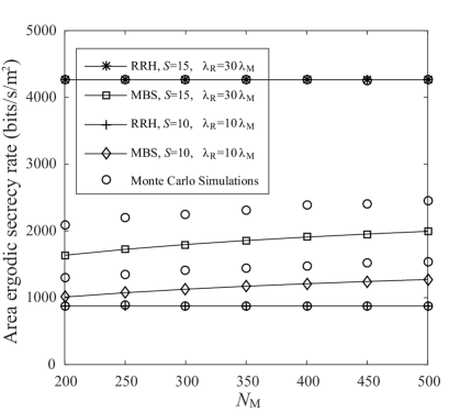
Figure 2: Effects of massive MIMO on the area ergodic secrecy rate: $\lambda_{\mathrm{M}}=\left(500^{2}\times\pi\right)^{-1}\mathrm{m}^{-2}$, $\lambda_{e}=10^{-5}$ m^-2, $\eta_{\mathrm{M}}=3.0$, $\eta_{\mathrm{R}}=3.6$, and $\alpha=0.5$.

Fig. 2 analyzes the effects of massive MIMO on the area ergodic secrecy rate. The analytical curves for area ergodic secrecy rate of the RRH tier were obtained from (22), which have a precise match to the results obtained using the Monte-Carlo simulations marked by ‘$\circ$’. The lower bound curves for area ergodic secrecy rate of the MBS tier were obtained from using (27), which can efficiently predict the performance behavior. As mentioned in Remark 3 of Section III-A, we observe that the area ergodic secrecy rate increases with the number of MBS antennas, due to more array gains obtained by the legitimate user. Increasing the number of served users can also significantly improve the ergodic secrecy rate. The area ergodic secrecy rate of the RRH tier remains unchanged with increasing the number of MBS antennas, since employing more MBS antennas will not cause more interference in the network. Nevertheless, it will substantially increase with the density of RRHs.

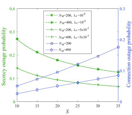
Figure 3: The secrecy outage probability and connection outage probability for MBS transmission in delay-limited mode: $R=8$ bits/s/Hz, $R_{\mathrm{s}}=0.3R$, $d_{o}=50$ m, $\lambda_{\mathrm{M}}=\left(500^{2}\times\pi\right)^{-1}\mathrm{m}^{-2}$, $\lambda_{\mathrm{R}}=20\times\lambda_{\mathrm{M}}$, $\eta_{\mathrm{M}}=3.0$ and $\eta_{\mathrm{R}}=3.6$.

Fig. 3 provides the results for the secrecy outage probability and connection outage probability of MBS transmission operating in delay-limited mode. With increasing the number of served users, the secrecy outage probability decreases and the connection outage probability increases. The reason is that the transmit power allocated to each user data stream decreases when serving more users at the MBS, which in turn decreases the receive SINR at both the legitimate user and eavesdroppers. To decrease the connection outage probability without altering the secrecy outage probability, MBSs can be equipped with more antennas to provide larger array gains for the legitimate users. In addition, it is obvious that more eavesdroppers will deteriorate the secrecy performance.

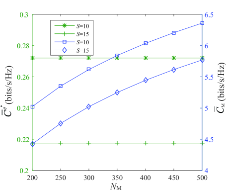
Figure 4: The ergodic capacity $\bar{C}^{e^{*}}$ of the most malicious eavesdropper’s channel and the ergodic capacity $\bar{C}_{\mathrm{M}}$ of the macrocell user’s channel for MBS transmission in delay-tolerant mode: $\lambda_{\mathrm{M}}=\left(500^{2}\times\pi\right)^{-1}\mathrm{m}^{-2}$, $\lambda_{\mathrm{R}}=20\times\lambda_{\mathrm{M}}$, $\lambda_{e}=10^{-5}$ m^-2, $\eta_{\mathrm{M}}=3.3$.

Fig. 4 shows the ergodic capacity $\bar{C}^{e^{*}}$ of the most malicious eavesdropper’s channel and the ergodic capacity $\bar{C}_{\mathrm{M}}$ of the macrocell user’s channel for MBS transmission in delay-tolerant mode. When adding more MBS antennas, $\bar{C}^{e^{*}}$ is unaltered and $\bar{C}_{\mathrm{M}}$ experiences a substantial increase, since only the legitimate macrocell users can obtain the array gains. Additionally, serving more users at the MBS decreases $\bar{C}^{{e^{\rm{*}}}}$ and $\bar{C}_{\mathrm{M}}$, because of lower transmit power per user data stream at the MBS as mentioned in Fig 3.

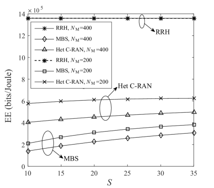
Figure 5: Effects of massive MIMO on the EE: $\lambda_{\mathrm{M}}=\left(500^{2}\times\pi\right)^{-1}\mathrm{m}^{-2}$, $\lambda_{\mathrm{R}}=20\times\lambda_{\mathrm{M}}$, $\eta_{\mathrm{M}}=3.2$, $\eta_{\mathrm{R}}=3.6$, and $\alpha=0.5$.

Fig. 5 illustrates the effects of massive MIMO on the EE. Results indicate that the EE of MBS transmission is improved by serving more users at the MBS, which is attributed to the fact that more multiplexing gain is achieved. Although adding more antennas at the MBS can provide a large array gain, there is a significant increase in power consumption resulting from massive MIMO baseband processing, which decreases the EE of MBS transmission. In addition, the RRHs achieve higher EE than the MBSs, as they use lower transmit power and do not consume power for baseband processing, and results also demonstrate that massive MIMO has negligible effect on the EE of RRH transmission.

V-B The Effects of RRH Density

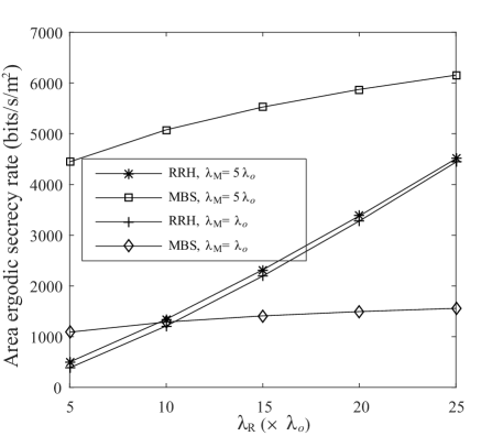
Figure 6: Effects of RRH density on area ergodic secrecy rate: $\lambda_{o}=\left(500^{2}\times\pi\right)^{-1}\mathrm{m}^{-2}$, $\lambda_{e}=10^{-5}\mathrm{m}^{-2}$, $N_{\mathrm{M}}=400$, $S=30$, $\eta_{\mathrm{M}}=3.0$, $\eta_{\mathrm{R}}=3.6$, and $\alpha=0.7$.

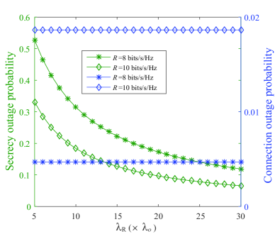
(a) $R_{s}=0.2R$, $d_{o}=30$ m, $\lambda_{o}=\left(500^{2}\times\pi\right)^{-1}\mathrm{m}^{-2}$, $\lambda_{e}=10^{-4}\mathrm{m}^{-2}$, $\eta_{\mathrm{R}}=3.6$.

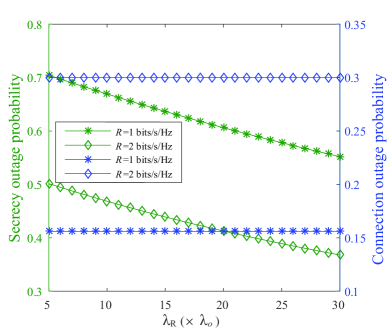
(b) $R_{s}=0.2R$, $d_{o}=30$ m, $\lambda_{\mathrm{M}}=\lambda_{o}=\left(500^{2}\times\pi\right)^{-1}\mathrm{m}^{-2}$, $\lambda_{e}=10^{-4}\mathrm{m}^{-2}$, $N_{\mathrm{M}}=200$, $S=15$, $\eta_{\mathrm{M}}=3.0$, and $\eta_{\mathrm{R}}=3.6$.

Figure 7: Secrecy outage probability and connection outage probability for RRH transmission in delay-limited mode.

Fig. 6 shows the effects of RRH density on area ergodic secrecy rate. We observe that when more RRHs are deployed, there is a substantial increase in the area ergodic secrecy rate of the RRH tier, as illustrated in Remark 2 of Section III-A. The area ergodic secrecy rate of the MBS tier can also increase with the density of RRH, since users with far-away MBSs will be offloaded to the RRHs. RRH tier can achieve higher area ergodic secrecy rate than the massive MIMO aided MBS tier when the RRHs are denser than the MBSs. In addition, slightly increasing the number of massive MIMO macrocells brings large improvement in the area ergodic secrecy rate of the MBS tier because more users can be served, and it also improves the area ergodic secrecy rate of the RRH tier due to the fact that users with far-away RRHs will be offloaded to the MBSs.

Fig. 7 shows the secrecy outage probability and connection outage probability of RRH transmission in delay-limited mode. Specifically, Fig. 7(a) focuses on the performance when RRH transmissions operate over the RBs only allocated to RRHs, while Fig. 7(b) concentrates on the performance when RRH transmissions operate over the RBs shared by RRHs and MBSs. As stated in Remark 5 of Section III-B, the secrecy outage probability experiences a massive decline when increasing the density of RRHs, due to more severe interference on the Eves but the connection outage probability is unaltered since the inter-RRH interference is mitigated in the C-RAN, as mentioned in Remark 4. Compared with the use of RBs shared by RRHs and MBSs, RRH achieves better performance by using the RBs only used by RRHs, due to the absence of inter-tier interference in these RBs.

Fig. 8 shows the ergodic capacity $\bar{C}^{e^{*}}$ of the most malicious eavesdropper’s channel and the ergodic capacity $\bar{C}_{\mathrm{R}}$ of the C-RAN user’s channel for RRH transmission in delay-tolerant mode. As suggested in Remark 2, deploying more RRHs can significantly decrease $\bar{C}^{e^{*}}$ and increase $\bar{C}_{\mathrm{R}}$. For RRH transmission over the RB shared by RRHs and MBSs, interference from the MBS tier has a large negative impact on the performance at the legitimate users, however, its impact on the degradation of the most malicious eavesdropper’s channel is limited compared to more interference from dense RRHs.

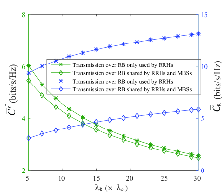
Figure 8: The ergodic capacity $\bar{C}^{e^{*}}$ of the most malicious eavesdropper’s channel and the ergodic capacity $\bar{C}_{\mathrm{R}}$ of the C-RAN user’s channel for RRH transmission in delay-tolerant mode: $\lambda_{\mathrm{M}}=\lambda_{o}=\left(500^{2}\times\pi\right)^{-1}\mathrm{m}^{-2}$, $\lambda_{e}=10^{-4}$ m^-2, $N_{\mathrm{M}}=200$, $S=15$, $\eta_{\mathrm{M}}=3.5$, and $\eta_{\mathrm{R}}=3.2$.

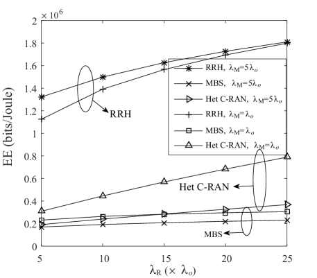
Figure 9: Effects of RRH density on the EE: $\lambda_{o}=\left(500^{2}\times\pi\right)^{-1}\mathrm{m}^{-2}$, $N_{\mathrm{M}}=400$, $S=30$, $\eta_{\mathrm{M}}=3.0$, $\eta_{\mathrm{R}}=3.6$, and $\alpha=0.7$.

Fig. 9 shows the effects of RRH density on the EE. As mentioned in Corollary 2 of Section IV, when increasing the density of RRHs, the EE of RRH transmission is significantly improved. Increasing the density of MBSs improves the EE of RRH transmission but decreases the EE of MBS transmission, since users with far-away RRHs are offloaded to the MBSs. The EE of the Het C-RAN decreases with increasing the density of MBSs, due to the fact that power consumption of the network is significantly boosted by using more massive MIMO MBSs. Since RRHs achieve higher EE, more RRHs should be deployed in the Het C-RAN to enhance the EE.

V-C The Effects of S-FFR

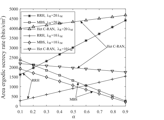
Figure 10: Effects of S-FFR on area ergodic secrecy rate: $\lambda_{\mathrm{M}}=\left(500^{2}\times\pi\right)^{-1}\mathrm{m}^{-2}$, $\lambda_{e}=5*10^{-5}$ m^-2, $N_{\mathrm{M}}=400$, $S=25$, $\eta_{\mathrm{M}}=3.5$, and $\eta_{\mathrm{R}}=3.3$.

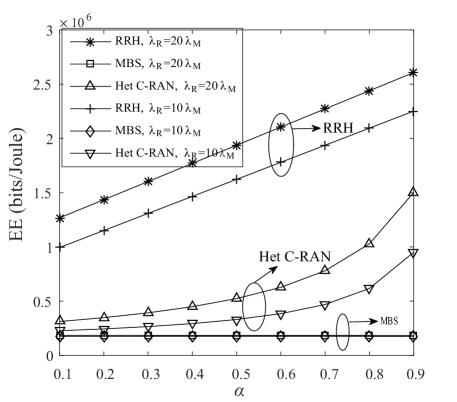
Figure 11: Effects of S-FFR on the EE: $\lambda_{\mathrm{M}}=\left(500^{2}\times\pi\right)^{-1}\mathrm{m}^{-2}$, $\lambda_{e}=5*10^{-5}$ m^-2, $N_{\mathrm{M}}=400$, $S=25$, $\eta_{\mathrm{M}}=3.5$, and $\eta_{\mathrm{R}}=3.3$.

Results in Fig. 10 demonstrate the effects of S-FFR on area ergodic secrecy rate. It is obvious that with more RBs allocated to the RRHs, the area ergodic secrecy rate increases for the RRH tier, and decreases for the MBS tier. The RRH tier can achieve higher area ergodic secrecy rate than the MBS tier, when the density of RRHs and the allocated RBs are large. More importantly, it is implied that the effect of S-FFR on the area ergodic secrecy rate of the network can be distinct depending on the RRH density.

Finally, Fig. 11 provides the effects of S-FFR on the EE. As mentioned in section IV, the EE for RRH transmission is indeed linearly improved by allocating more RBs to the RRHs without the harm of inter-tier interference. S-FFR indeed has little effect on the EE of MBS transmission. Therefore, the EE of the network increases with the RRH density and RBs only used by RRHs, as shown in this figure.

VI Conclusions

In this paper, we investigated the physical layer secrecy and EE in the two-tier massive MIMO aided heterogeneous C-RAN, where massive MIMO empowered macrocell BSs and RRHs coexist. The implementation of S-FFR was utilized to suppress the inter-tier interference. We first studied the impacts of massive MIMO and C-RAN on the secrecy performance in terms of the area ergodic secrecy rate and secrecy outage probability. Then we evaluated the EE in such networks. Our results demonstrated that both C-RAN and massive MIMO can significantly enhance the secrecy performance. The implementation of C-RAN with low power cost RRHs improves EE of the networks substantially.

Appendix A: A detailed derivation of Theorem 1

When using the $k$-th RB allocated to the RRHs, the ergodic capacity of the channel between the typical RRH and its served user is given by

$$\bar{C}_{\mathrm{R},k}={\mathbb{E}}\left\{\log_{2}\left(1+\gamma_{\mathrm{R},k}\right)\right\}$$

$$=\int_{0}^{\infty}{\mathbb{\mathrm{E}}}_{h_{\mathrm{R},k}}\left\{\log_{2}\left(1+\frac{P_{\mathrm{R}}\beta}{B_{o}N_{o}}h_{\mathrm{R},k}x^{-\eta_{\mathrm{R}}}\right)\right\}f_{\left|{{X_{{o},\mathrm{R}}}}\right|}\left(x\right)dx.$$ (A.1)

Considering that $h_{\mathrm{R},k}\sim\rm{exp}(1)$, we further have

$$\bar{C}_{\mathrm{R},k} =\frac{1}{{\ln 2}}\int_{0}^{\infty}{\left\{{\int_{\rm{0}}^{\infty}{\frac{1}{{1+t}}}{e^{-\frac{{{B_{o}}{N_{o}}}}{{{P_{\rm{R}}}\beta}}{x^{{\eta_{\rm{R}}}}}t}}dt}\right\}{f_{\left|{{X_{o,{\rm{R}}}}}\right|}}\left(x\right)dx}$$

$$=\frac{1}{{\ln 2}}\int_{0}^{\infty}{{e^{\frac{{{B_{o}}{N_{o}}}}{{{P_{\rm{R}}}\beta}}{x^{{\eta_{\rm{R}}}}}}}\Gamma\left({0,\frac{{{B_{o}}{N_{o}}}}{{{P_{\rm{R}}}\beta}}{x^{{\eta_{\rm{R}}}}}}\right){f_{\left|{{X_{o,{\rm{R}}}}}\right|}}\left(x\right)dx},$$ (A.2)

where ${f_{\left|{{X_{o,{\rm{R}}}}}\right|}}\left(x\right)$ is the probability density function (PDF) of the distance between the typical RRH and its intended user, using the similar approach in [30], ${f_{\left|{{X_{o,{\rm{R}}}}}\right|}}\left(x\right)$ is given by

$${f_{\left|{{X_{o,{\rm{R}}}}}\right|}}\left(x\right)=\frac{{2\pi{\lambda_{\mathrm{R}}}}}{{{\mathcal{A}_{\mathrm{R}}}}}x{e^{-\pi\left({{\lambda_{\mathrm{R}}}+{\lambda_{\mathrm{M}}}}\right){x^{2}}}},$$ (A.3)

where ${\mathcal{A}_{\mathrm{R}}}=\frac{\lambda_{\mathrm{R}}}{\lambda_{\mathrm{R}}+\lambda_{\mathrm{M}}}$ is the probability that a user is associated with the RRH. By plugging (A.3) into (Appendix A: A detailed derivation of Theorem 1), we get (13).

When using the $\nu$-th RB shared by the RRHs and MBSs, the ergodic capacity of the channel between the typical RRH and its served user is given by

$$\bar{C}_{\mathrm{R},\nu} ={\mathbb{E}}\left\{\log_{2}\left(1+\gamma_{\mathrm{R},\nu}\right)\right\}$$

$$=\frac{1}{{\ln 2}}\int_{0}^{\infty}{{\mathbb{E}}_{\left|{{X_{o,{\rm{R}}}}}\right|=x}\left\{\log_{2}\left(1+\gamma_{\mathrm{R},\nu}\right)\right\}{f_{\left|{{X_{o,{\rm{R}}}}}\right|}}\left(x\right)dx}$$

$$=\frac{1}{{\ln 2}}\int_{0}^{\infty}{\left[{\int_{0}^{\infty}{\frac{{\bar{F}}_{{\gamma_{\mathrm{R},\nu}}\mid\left\{\left|{{X_{o,{\rm{R}}}}}\right|=x\right\}}\left(\gamma\right)}{{1+\gamma}}d\gamma}}\right]{f_{\left|{{X_{o,{\rm{R}}}}}\right|}}\left(x\right)dx},$$ (A.4)

where ${\bar{F}}_{{\gamma_{\mathrm{R},\nu}}\mid\left\{\left|{{X_{o,{\rm{R}}}}}\right|=x\right\}}\left(\gamma\right)$ is the CCDF of $\gamma_{\mathrm{R},\nu}$ given a distance $\left|{{X_{o,{\rm{R}}}}}\right|=x$, which is calculated as

$${\bar{F}}_{{\gamma_{\mathrm{R},\nu}}\mid\left\{\left|{{X_{o,{\rm{R}}}}}\right|=x\right\}}\left(\gamma\right)=\Pr\left({\frac{{{P_{\rm{R}}}{h_{{\rm{R}},\nu}}\beta{x^{-{\eta_{\rm{R}}}}}}}{{{I_{{\rm{M}},\nu}}+{B_{o}}{N_{o}}}}>\gamma}\right)$$

$$={e^{-\frac{{{B_{o}}{N_{o}}}}{{{P_{\rm{R}}}\beta}}{x^{{\eta_{\rm{R}}}}}\gamma}}{\mathbb{\mathrm{E}}_{{\Phi_{\mathrm{M}}}}}\left\{{{e^{-\frac{1}{{{P_{\rm{R}}}\beta}}{x^{{\eta_{\rm{R}}}}}\gamma{I_{{\rm{M}},\nu}}}}}\right\}$$

$$={e^{-\frac{{{B_{o}}{N_{o}}}}{{{P_{\rm{R}}}\beta}}{x^{{\eta_{\rm{R}}}}}\gamma}}\mathcal{L}_{{I_{{\rm{M}},\nu}}}\left({\frac{1}{{{P_{\rm{R}}}\beta}}{x^{{\eta_{\rm{R}}}}}\gamma}\right),$$ (A.5)

where $\mathcal{L}_{{I_{{\rm{M}},\nu}}}\left(\cdot\right)$ is the laplace transform of the PDF of ${I_{{\rm{M}},\nu}}$, and is given by

$$\mathcal{L}_{{I_{{\rm{M}},\nu}}}\left(s\right)=\mathbb{\mathrm{E}}\left\{\exp\left\{-\left(\sum\limits_{\ell\in{\Phi_{\mathrm{M}}}}{\frac{P_{\mathrm{M}}}{S}{h_{\ell,\nu}}\beta\left|{{X_{\ell,\mathrm{M}}}}\right|^{-\eta_{\mathrm{M}}}}\right)s\right\}\right\}$$

$$\mathop{=}\limits^{\left(b\right)}\exp\left\{{-\int_{x}^{\infty}{\left({1-\frac{1}{{{{\left({1+s\frac{{{P_{\mathrm{M}}}}}{S}\beta{r^{-{\eta_{\mathrm{M}}}}}}\right)}^{S}}}}}\right){\lambda_{\mathrm{M}}}2\pi rdr}}\right\}$$

$$\mathop{=}\limits^{\left(c\right)}\exp\left({-{\lambda_{\mathrm{M}}}2\pi\sum\limits_{\mu=1}^{S}{S\choose\mu}\int_{x}^{\infty}{\frac{{{{{{\left({\frac{{{P_{\rm{M}}}}}{S}\beta}\right)}^{\mu}}{s^{\mu}}\left({{r^{-{\eta_{\mathrm{M}}}}}}\right)}^{\mu}}}}{{{{\left({1+s\frac{{{P_{\mathrm{M}}}}}{S}\beta{r^{-{\eta_{\mathrm{M}}}}}}\right)}^{S}}}}rdr}}\right)$$

$$=\exp\bigg{\{}-{\lambda_{\mathrm{M}}}2\pi\sum\limits_{\mu=1}^{S}{{S\choose\mu}{{\left({s\frac{{{P_{\mathrm{M}}}}}{{S}}}\beta\right)}^{\mu}}}\frac{{{{\left({-s\frac{{{P_{\mathrm{M}}}}}{{S}}}\beta\right)}^{-\mu+\frac{2}{{{\eta_{\mathrm{M}}}}}}}}}{{{\eta_{\mathrm{M}}}}}$$

$$\;\;\;{B_{\left(-{s\frac{{{P_{\mathrm{M}}}}}{{S}}\beta x^{-\eta_{\mathrm{M}}}}\right)}}\left[{\mu-\frac{2}{{{\eta_{\mathrm{M}}}}},1-S}\right]\bigg{\}},$$ (A.6)

where (b) is obtained by using the generating functional of PPP [31], (c) results from using Binomial expansion, $\mathrm{B}_{\left(\cdot\right)}\left[\cdot,\cdot\right]$ is the incomplete beta function [21, (8.391)]. By pulling (Appendix A: A detailed derivation of Theorem 1) and (Appendix A: A detailed derivation of Theorem 1) together, we get (III-A). Substituting (A.3) into (Appendix A: A detailed derivation of Theorem 1), we also get (14).

Appendix B: A detailed derivation of Theorem 2

The ergodic capacity $\bar{C}_{\mathrm{R},i}^{e^{*}}$ $(i\in\left\{k,\nu\right\})$ of the most malicious eavesdropper’s channel is written as

$$\bar{C}_{\mathrm{R},i}^{e^{*}} ={\mathbb{E}}\left\{\log_{2}\left(1+\gamma_{\mathrm{R},i}^{e^{*}}\right)\right\}$$

$$=\frac{1}{{\ln 2}}\int_{0}^{\infty}\frac{1-F_{\gamma_{\mathrm{R},i}^{e^{*}}}\left(x\right)}{1+x}dx,$$ (B.1)

where $F_{\gamma_{\mathrm{R},i}^{e^{*}}}\left(x\right)$ denotes the cumulative distribution function (CDF) of ${\gamma_{\mathrm{R},i}^{e^{*}}}$.

Based on (4), the CDF of ${\gamma_{\mathrm{R},k}^{e^{*}}}$ is calculated as

$$F_{\gamma_{\mathrm{R},k}^{e^{*}}}\left(x\right)=\Pr\left(\gamma_{\mathrm{R},k}^{e^{*}}<x\right)$$

$$=\Pr\left(\mathop{\max}\limits_{e\in\Phi_{e}}\left\{\frac{{{P_{\mathrm{R}}}h_{\mathrm{R}{\rm{,}}k}^{e}\beta{{\left|{X_{o{\rm{,}}\mathrm{R}}^{e}}\right|}^{-{\eta_{\mathrm{R}}}}}}}{{I_{\mathrm{R},k}^{e}+{B_{o}}{N_{e}}}}\right\}<x\right)$$

$$=\mathbb{E}_{\Phi_{e}}\bigg{\{}\prod\limits_{e\in{\Phi_{e}}}{\Pr\left(\frac{{{P_{\mathrm{R}}}h_{\mathrm{R}{\rm{,}}k}^{e}\beta{{\left|{X_{o{\rm{,}}\mathrm{R}}^{e}}\right|}^{-{\eta_{\mathrm{R}}}}}}}{{I_{\mathrm{R},k}^{e}+{B_{o}}{N_{e}}}}<x\left.\right|\Phi_{e}\right)}\bigg{\}}.$$ (B.2)

Using the generating functional of the PPP $\Phi_{e}$, $F_{\gamma_{\mathrm{R},k}^{e^{*}}}\left(x\right)$ can be further derived as

$$F_{\gamma_{\mathrm{R},k}^{e^{*}}}\left(x\right)=\exp\bigg{\{}-{\lambda_{e}}\int_{{R^{\rm{2}}}}\Big{(}1-{\Pr\Big{(}\frac{{{P_{\mathrm{R}}}h_{\mathrm{R}{\rm{,}}k}^{e}\beta{{r}^{-{\eta_{\mathrm{R}}}}}}}{{I_{\mathrm{R},k}^{e}+{B_{o}}{N_{e}}}}<x\Big{)}}\Big{)}{dr}\Big{\}}$$

$$=\exp\bigg{\{}-{\lambda_{e}}\int_{{R^{\rm{2}}}}\mathbb{E}_{\Phi_{\mathrm{R}}}\bigg{\{}\mathbb{E}_{\Phi_{\mathrm{M}}}\bigg{\{}$$

$$\quad\quad\quad\quad\quad\;\;\exp\big{[}-\frac{{r}^{{\eta_{\mathrm{R}}}}x}{{P_{\mathrm{R}}}\beta}\left(I_{\mathrm{R},k}^{e}+{B_{o}}{N_{e}}\right)\big{]}\bigg{\}}\bigg{\}}dr\bigg{\}}$$

$$\mathop{=}\limits^{\left(a\right)}\exp\bigg{\{}-2\pi{\lambda_{e}}\int_{0}^{\infty}\exp\big{[}-\frac{{r}^{{\eta_{\mathrm{R}}}}x}{{P_{\mathrm{R}}}\beta}{B_{o}}{N_{e}}\big{]}\mathcal{L}_{I_{\mathrm{R},k}^{e}}\big{(}\frac{{r}^{{\eta_{\mathrm{R}}}}x}{{P_{\mathrm{R}}}\beta}\big{)}rdr\bigg{\}},$$ (B.3)

where (a) results from using the polar-coordinate system, $\mathcal{L}_{I_{\mathrm{R},k}^{e}}\left(\cdot\right)$ is the laplace transform of the PDF of ${I_{\mathrm{R},k}^{e}}$.

Likewise, the CDF of ${\gamma_{\mathrm{R},\nu}^{e^{*}}}$ is calculated as

$$F_{\gamma_{\mathrm{R},\nu}^{e^{*}}}\left(x\right)=\Pr\left(\gamma_{\mathrm{R},\nu}^{e^{*}}<x\right)$$

$$=\Pr\left(\mathop{\max}\limits_{e\in\Phi_{e}}\left\{\frac{{{P_{\mathrm{R}}}h_{\mathrm{R}{\rm{,}}\nu}^{e}\beta{{\left|{X_{o{\rm{,}}\mathrm{R}}^{e}}\right|}^{-{\eta_{\mathrm{R}}}}}}}{{I_{\mathrm{R},\nu}^{e}+I_{\mathrm{M},\nu}^{e}+{B_{o}}{N_{e}}}}\right\}<x\right)$$

$$=\mathbb{E}_{\Phi_{e}}\bigg{\{}\prod\limits_{e\in{\Phi_{e}}}{\Pr\left(\frac{{{P_{\mathrm{R}}}h_{\mathrm{R}{\rm{,}}\nu}^{e}\beta{{\left|{X_{o{\rm{,}}\mathrm{R}}^{e}}\right|}^{-{\eta_{\mathrm{R}}}}}}}{{I_{\mathrm{M},\nu}^{e}+I_{\mathrm{R},\nu}^{e}+{B_{o}}{N_{e}}}}<x\left.\right|\Phi_{e}\right)}\bigg{\}}$$

$$=\exp\bigg{\{}-2\pi{\lambda_{e}}\int_{0}^{\infty}\exp\big{[}-\frac{{r}^{{\eta_{\mathrm{R}}}}x}{{P_{\mathrm{R}}}\beta}{B_{o}}{N_{e}}\big{]}$$

$$\quad\quad\quad\quad\quad\quad\quad\quad\mathcal{L}_{I_{\mathrm{R},\nu}^{e}}\big{(}\frac{{r}^{{\eta_{\mathrm{R}}}}x}{{P_{\mathrm{R}}}\beta}\big{)}\mathcal{L}_{I_{\mathrm{M},\nu}^{e}}\big{(}\frac{{r}^{{\eta_{\mathrm{R}}}}x}{{P_{\mathrm{R}}}\beta}\big{)}rdr\bigg{\}},$$ (B.4)

where $\mathcal{L}_{I_{\mathrm{R},\nu}^{e}}\left(\cdot\right)$ and $\mathcal{L}_{I_{\mathrm{M},\nu}^{e}}\left(\cdot\right)$ are the laplace transforms of the PDFs of ${I_{\mathrm{R},\nu}^{e}}$ and ${I_{\mathrm{M},\nu}^{e}}$, respectively.

By using the Slivnyak’s theorem and the generating functional of the PPP $\Phi_{R}$, $\mathcal{L}_{I_{\mathrm{R},i}^{e}}\left(\cdot\right)$ $(i\in\left\{k,\nu\right\})$ is given by

$$\mathcal{L}_{I_{\mathrm{R},i}^{e}}\left(s\right)=\mathbb{E}\left\{\exp\left(-sI_{\mathrm{R},i}^{e}\right)\right\}$$

$$=\exp\left(-2\pi\lambda_{\mathrm{R}}\int_{0}^{\infty}\left(1-\frac{1}{\left(1+sP_{\mathrm{R}}\beta r^{-\eta_{\mathrm{R}}}\right)}\right)rdr\right)$$

$$=\exp\left(-\lambda_{\mathrm{R}}\pi\left(P_{\mathrm{R}}\beta\right)^{\frac{2}{\eta_{\mathrm{R}}}}\Gamma\left(1+\frac{2}{\eta_{\mathrm{R}}}\right)\Gamma\left(1-\frac{2}{\eta_{\mathrm{R}}}\right)s^{\frac{2}{\eta_{\mathrm{R}}}}\right).$$ (B.5)

Similarly, ${I_{\mathrm{M},\nu}^{e}}$ is given by

$$\mathcal{L}_{I_{\mathrm{M},\nu}^{e}}\left(s\right) =\exp\left[-2\pi\lambda_{\mathrm{M}}\int_{0}^{\infty}\left(1-\frac{1}{\left(1+s\frac{P_{\mathrm{M}}}{S}\beta r^{-\eta_{\mathrm{M}}}\right)^{S}}\right)rdr\right]$$

$$=\exp\bigg{[}-2\pi\lambda_{\mathrm{M}}\sum\limits_{\mu=1}^{S}{S\choose\mu}\left(s\frac{P_{\mathrm{M}}}{S}\beta\right)^{\frac{2}{\eta_{\mathrm{M}}}}$$

$$\quad\quad\quad\quad\frac{\Gamma\left(\mu-\frac{2}{\eta_{\mathrm{M}}}\right)\Gamma\left(-\mu+\frac{2}{\eta_{\mathrm{M}}}+S\right)}{\eta_{\mathrm{M}}\Gamma\left(S\right)}\bigg{]}.$$ (B.6)

Substituting (Appendix B: A detailed derivation of Theorem 2) into (Appendix B: A detailed derivation of Theorem 2), we get $F_{\gamma_{\mathrm{R},k}^{e^{*}}}\left(\cdot\right)$ as (17). Then, substituting (Appendix B: A detailed derivation of Theorem 2) and (Appendix B: A detailed derivation of Theorem 2) into (Appendix B: A detailed derivation of Theorem 2), we get $F_{\gamma_{\mathrm{R},\nu}^{e^{*}}}\left(\cdot\right)$ as (III-A).

Appendix C: A detailed derivation of Theorem 3

The ergodic capacity of the channel between the typical MBS and its served user is written as

$$\bar{C}_{\mathrm{M},\nu}=\mathbb{E}\left\{\log_{2}\left(1+\gamma_{\mathrm{M},\nu}\right)\right\}.$$ (C.1)

By using Jensen’s inequality, a tight lower bound for $\bar{C}_{\mathrm{M},\nu}$ is given by [25]

$$\bar{C}_{\mathrm{M},\nu}^{\mathrm{L}}=\log_{2}\left(1+e^{Z_{3}+Z_{4}}\right),$$ (C.2)

where

$$Z_{3}=\mathbb{\mathrm{E}}\left\{\ln\left(\frac{P_{\mathrm{M}}}{S}g_{\mathrm{M},\nu}\beta\left|{{X_{{o},\mathrm{M}}}}\right|^{-\eta_{\mathrm{M}}}\right)\right\},$$ (C.3)

and

$$Z_{4}=\mathbb{\mathrm{E}}\left\{\ln\left(\frac{1}{J_{\mathrm{M},\nu}+J_{\mathrm{R},\nu}+B_{o}N_{1}}\right)\right\}.$$ (C.4)

We first calculate $Z_{3}$ as

$$Z_{3}=\ln\left({\frac{{{P_{\rm{M}}}}}{S}\beta}\right){\rm{+}}\mathbb{\mathrm{E}}\left\{{\ln\left({{g_{{\rm{M}},\nu}}}\right)}\right\}-{\eta_{\rm{M}}}\mathbb{\mathrm{E}}\left\{{\ln\left({\left|{{X_{o,{\rm{M}}}}}\right|}\right)}\right\}.$$ (C.5)

Considering that $g_{\mathrm{M},\nu}\sim\Gamma\left(N_{\mathrm{M}}-S+1,1\right)$, $\mathbb{\mathrm{E}}\left\{{\ln\left({{g_{{\rm{M}},\nu}}}\right)}\right\}$ is given by

$$\mathbb{\mathrm{E}}\left\{{\ln\left({{g_{{\rm{M}},\nu}}}\right)}\right\} =\int_{0}^{\infty}{\frac{{{x^{N_{\mathrm{M}}-S}}{e^{-x}}}}{{\left({N_{\mathrm{M}}-S}\right)!}}\ln\left(x\right)dx}$$

$$\mathop{=}\limits^{\left(a\right)}\psi\left(N_{\mathrm{M}}-S+1\right),$$ (C.6)

where (a) results from using $\int_{0}^{\infty}{{x^{v-1}}{e^{-\mu x}}\ln xdx}={\mu^{-v}}\Gamma\left(v\right)\left({\psi\left(v\right)-\ln\mu}\right)$ [21, (4.352.1)]. Then, $\mathbb{\mathrm{E}}\left\{{\ln\left({\left|{{X_{o,{\rm{M}}}}}\right|}\right)}\right\}$ is derived as

$$\mathbb{\mathrm{E}}\left\{{\ln\left({\left|{{X_{o,{\rm{M}}}}}\right|}\right)}\right\} \mathop{=}\limits^{\left(b\right)}\int_{0}^{\infty}{\ln\left(x\right){f_{\left|{{X_{o,{\rm{M}}}}}\right|}}\left(x\right)dx}$$

$$=\int_{0}^{\infty}{\ln\left(x\right)\frac{2\pi\lambda_{\mathrm{M}}}{{\mathcal{A}_{\mathrm{M}}}}x{e^{-\pi\left({{\lambda_{\mathrm{R}}}+{\lambda_{\mathrm{M}}}}\right){x^{2}}}}dx}$$

$$=\frac{1}{2}\left({\psi\left(1\right)-\ln\left({\pi\left({{\lambda_{\rm{R}}}+{\lambda_{\rm{M}}}}\right)}\right)}\right).$$ (C.7)

In (b) above, ${f_{\left|{{X_{o,{\rm{M}}}}}\right|}}\left(x\right)$ is the PDF of the distance between the typical MBS and its intended user, which can be directly obtained following (A.3), and ${\mathcal{A}_{\mathrm{M}}}=\frac{\lambda_{\mathrm{M}}}{\lambda_{\mathrm{R}}+\lambda_{\mathrm{M}}}$ is the probability that a user is associated with the MBS. By substituting (Appendix C: A detailed derivation of Theorem 3) and (Appendix C: A detailed derivation of Theorem 3) into (C.5), we obtain $Z_{3}$ as

$$Z_{3}= \ln\left({\frac{{{P_{\rm{M}}}}}{S}\beta}\right)+\psi\left(N_{\mathrm{M}}-S+1\right)$$

$$-\frac{\eta_{\rm{M}}}{2}\left(\psi\left(1\right)-\ln\left({\pi\left({{\lambda_{\rm{R}}}+{\lambda_{\rm{M}}}}\right)}\right)\right).$$ (C.8)

From (C.4), considering the convexity of $\ln\left(\frac{1}{1+x}\right)$ and using Jensen’s inequality, we derive the lower bound on the $Z_{4}$ as

$$Z_{4}\geq\bar{Z}_{4}=\ln\left(\frac{1}{\mathbb{\mathrm{E}}\left\{J_{\mathrm{M},\nu}\right\}+\mathbb{\mathrm{E}}\left\{J_{\mathrm{R},\nu}\right\}+B_{o}N_{1}}\right).$$ (C.9)

Then, we have

$$\mathbb{\mathrm{E}}\left\{J_{\mathrm{M},\nu}\right\}= \int_{0}^{\infty}\mathbb{\mathrm{E}}\left\{\sum\limits_{\ell\in{\Phi_{\mathrm{M}}}/{o}}{\frac{P_{\mathrm{M}}}{S}{g_{\ell,\nu}}\beta\left|{{X_{\ell,\mathrm{M}}}}\right|^{-\eta_{\mathrm{M}}}}\right\}{f_{\left|{{X_{o,{\rm{M}}}}}\right|}}\left(x\right)dx$$

$$\mathop{=}\limits^{\left(c\right)} \int_{0}^{\infty}\left({P_{\mathrm{M}}}\beta 2\pi{\lambda_{\mathrm{M}}}\int_{x}^{\infty}r^{1-\eta_{\mathrm{M}}}dr\right){f_{\left|{{X_{o,{\rm{M}}}}}\right|}}\left(x\right)dx$$

$$= {\frac{{{P_{\mathrm{M}}}\beta 2\pi{\lambda_{\mathrm{M}}}}\Gamma\left(2-\frac{\eta_{\mathrm{M}}}{2}\right)}{{\left({\eta_{\mathrm{M}}}-2\right)\left(\pi\lambda_{\mathrm{M}}+\pi\lambda_{\mathrm{R}}\right)^{1-\frac{\eta_{\mathrm{M}}}{2}}}}},$$ (C.10)

where (c) results from using Campbell’s theorem [32]. Likewise, $\mathbb{\mathrm{E}}\left\{J_{\mathrm{R},\nu}\right\}$ is calculated as

$$\mathbb{\mathrm{E}}\left\{J_{\mathrm{R},\nu}\right\}= \int_{0}^{\infty}\mathbb{\mathrm{E}}\left\{\sum\limits_{j\in{\Phi_{\mathrm{R}}}}{{P_{\mathrm{R}}}{g_{j,\nu}}\beta\left|{{X_{j,\mathrm{R}}}}\right|^{-\eta_{\mathrm{R}}}}\right\}{f_{\left|{{X_{o,{\rm{M}}}}}\right|}}\left(x\right)dx$$

$$= {\frac{{{P_{\mathrm{R}}}\beta 2\pi{\lambda_{\mathrm{R}}}}\Gamma\left(2-\frac{\eta_{\mathrm{R}}}{2}\right)}{{\left({\eta_{\mathrm{R}}}-2\right)\left(\pi\lambda_{\mathrm{M}}+\pi\lambda_{\mathrm{R}}\right)^{1-\frac{\eta_{\mathrm{R}}}{2}}}}}.$$ (C.11)

Substituting (Appendix C: A detailed derivation of Theorem 3) and (C.9) into (C.2), we obtain (3).

Appendix D: A detailed derivation of Corollary 1

When the connection outage constraint $P_{\mathrm{R},k}^{\mathrm{co}}\left(R\right)=\sigma$, using (III-B1), we can easily get (30).

For connection outage constraint on the RRH transmission over the $\nu$-th RB shared by RRHs and MBSs, namely $P_{\mathrm{R},\nu}^{\mathrm{co}}\left(R\right)=\sigma$, we have

$${\bar{F}}_{{\gamma_{\mathrm{R},\nu}}\mid\left\{\left|{{X_{o,{\rm{R}}}}}\right|=d_{o}\right\}}\left(2^{R}-1\right)=1-\sigma.$$ (D.1)

Since the noise can be ignored compared with the inter-tier interference from MBSs, based on (Appendix A: A detailed derivation of Theorem 1) and (Appendix A: A detailed derivation of Theorem 1), we consider the worse case that interferers are located everywhere in the plane and derive the lower bound for ${\bar{F}}_{{\gamma_{\mathrm{R},\nu}}\mid\left\{\left|{{X_{o,{\rm{R}}}}}\right|=d_{o}\right\}}\left(\cdot\right)$ as

$${\bar{F}}_{{\gamma_{\mathrm{R},\nu}}\mid\left\{\left|{{X_{o,{\rm{R}}}}}\right|=d_{o}\right\}}^{\mathrm{L}}\left(\gamma\right)$$

$$=\exp\left\{{-\int_{0}^{\infty}{\bigg{(}{1-\frac{1}{{{{\left({1+\frac{{{P_{\mathrm{M}}}d_{o}^{\eta_{\mathrm{R}}}\gamma}}{{P_{\mathrm{R}}}S}{r^{-{\eta_{\mathrm{M}}}}}}\right)}^{S}}}}}\bigg{)}{\lambda_{\mathrm{M}}}2\pi rdr}}\right\}$$

$$=\exp\bigg{(}-2\pi{\lambda_{\mathrm{M}}}{{\left({\frac{{{P_{\mathrm{M}}}{d_{o}^{{\eta_{\mathrm{R}}}}}}}{{{P_{\mathrm{R}}}S}}\gamma}\right)}^{\frac{2}{{{\eta_{\mathrm{M}}}}}}}\sum\limits_{\mu=1}^{S}{S\choose\mu}$$

$$\quad\quad\quad\quad\frac{{\Gamma\left({\mu-\frac{2}{{{\eta_{\mathrm{M}}}}}}\right)\Gamma\left({-\mu+\frac{2}{{{\eta_{\mathrm{M}}}}}+S}\right)}}{{{\eta_{\mathrm{M}}}\Gamma\left(S\right)}}\bigg{)}.$$ (D.2)

Substituting (Appendix D: A detailed derivation of Corollary 1) into (D.1), after some manipulations, we obtain (31).

References

• [1] A. Checko, H. Christiansen, Y. Yan, L. Scolari, G. Kardaras, M. Berger, and L. Dittmann, “Cloud RAN for mobile networks–a technology overview,” IEEE Commun. Surveys & Tutorials, vol. 17, no. 1, pp. 405–426, 2015.
• [2] H. Q. Ngo, E. G. Larsson, and T. L. Marzetta, “Energy and spectral efficiency of very large multiuser MIMO systems,” IEEE Trans. Commun., vol. 61, no. 4, pp. 1436–1449, Apr. 2013.
• [3] J. Andrews, S. Buzzi, W. Choi, S. Hanly, A. Lozano, A. Soong, and J. Zhang, “What will 5G be?” IEEE J. Sel. Areas Commun., vol. 32, no. 6, pp. 1065–1082, June 2014.
• [4] E. Hossain and M. Hasan, “5G cellular: Key enabling technologies and research challenges,” IEEE Instrumentation Measurement Mag., vol. 18, no. 3, pp. 11–21, Jun. 2015.
• [5] D. Liu, L. Wang, Y. Chen, M. Elkashlan, K. K. Wong, R. Schober, and L. Hanzo, “User association in 5G networks: A survey and an outlook,” IEEE Commun. Surveys & Tutorials, vol. 18, no. 2, pp. 1018–1044, 2016.
• [6] M. Peng, C. Wang, V. Lau, and H. Poor, “Fronthaul-constrained cloud radio access networks: insights and challenges,” IEEE Wireless Commun., vol. 22, no. 2, pp. 152–160, 2015.
• [7] Z. Ding and H. Poor, “The use of spatially random base stations in cloud radio access networks,” IEEE Signal Process. Lett., vol. 20, no. 11, pp. 1138–1141, Nov. 2013.
• [8] S. Zaidi, A. Imran, D. C. Mclernon, and M. Ghogho, “Characterizing coverage and downlink throughput of cloud empowered hetnets,” IEEE Commun. Lett., vol. 19, no. 6, pp. 1013–1016, June 2015.
• [9] F. Khan, H. He, J. Xue, and T. Ratnarajah, “Performance analysis of cloud radio access networks with distributed multiple antenna remote radio heads,” IEEE Trans. Signal Process., vol. 63, no. 18, pp. 4784–4799, Sep. 2015.
• [10] M. Peng, Y. Li, J. Jiang, J. Li, and C. Wang, “Heterogeneous cloud radio access networks: A new perspective for enhancing spectral and energy efficiencies,” IEEE Wireless Commun., vol. 21, no. 6, pp. 126–135, 2014.
• [11] M. Peng, K. Zhang, J. Jiang, J. Wang, and W. Wang, “Energy-efficient resource assignment and power allocation in heterogeneous cloud radio access networks,” IEEE Trans. Veh. Technol., pp. 1–13, 2015.
• [12] L. Dong, Z. Han, A. P. Petropulu, and H. V. Poor, “Improving wireless physical layer security via cooperating relays,” IEEE Trans. Signal Process., vol. 58, no. 3, pp. 1875–1888, Mar. 2010.
• [13] N. Yang, L. Wang, G. Geraci, M. Elkashlan, J. Yuan, and M. Di Renzo, “Safeguarding 5G wireless communication networks using physical layer security,” IEEE Commun. Mag., vol. 53, no. 4, pp. 20–27, Apr. 2015.
• [14] J. Zhu, R. Schober, and V. K. Bhargava, “Secure transmission in multicell massive MIMO systems,” IEEE Trans. Wireless Commun., vol. 13, no. 9, pp. 4766–4781, Sep. 2014.
• [15] D. Kapetanovic, G. Zheng, and F. Rusek, “Physical layer security for massive MIMO: An overview on passive eavesdropping and active attacks,” IEEE Commun. Mag., vol. 53, no. 6, pp. 21–27, June 2015.
• [16] G. Zheng, L.-C. Choo, and K.-K. Wong, “Optimal cooperative jamming to enhance physical layer security using relays,” IEEE Trans. Signal Process., vol. 59, no. 3, pp. 1317–1322, Mar. 2011.
• [17] J. Huang and A. L. Swindlehurst, “Cooperative jamming for secure communications in MIMO relay networks,” IEEE Trans. Signal Process., vol. 59, no. 10, pp. 4871–4884, Oct. 2011.
• [18] Z. Chu, K. Cumanan, Z. Ding, M. Johnston, and S. Le goff, “Secrecy Rate Optimizations for a MIMO Secrecy Channel with a Cooperative Jammer,” IEEE Trans. Veh. Technol., vol. 64, no. 5, pp. 1833-1847, May 2015.
• [19] G. Geraci, H. S. Dhillon, J. G. Andrews, J. Yuan, and I. B. Collings, “Physical layer security in downlink multi-antenna cellular networks,” IEEE Trans. Commun., vol. 62, no. 6, pp. 2006–2021, June 2014.
• [20] K. Hosseini, W. Yu, and R. S. Adve, “Large-scale MIMO versus network MIMO for multicell interference mitigation,” IEEE J. Sel. Topics Signal Process., vol. 8, no. 5, pp. 930–941, Oct. 2014.
• [21] I. S. Gradshteyn and I. M. Ryzhik, Table of Integrals, Series and Products, 7th ed.   San Diego, C.A.: Academic Press, 2007.
• [22] E. Björnson, L. Sanguinetti, J. Hoydis, and M. Debbah, “Designing multi-user MIMO for energy efficiency: When is massive MIMO the answer?” in Proc. 2014 IEEE WCNC, Apr. 2014.
• [23] X. Zhou and M. R. Mckay, “Secure transmission with artificial noise over fading channels: Achievable rate and optimal power allocation,” IEEE Trans. Veh. Technol., vol. 59, no. 8, pp. 3831–3842, Oct. 2010.
• [24] M. Abramowitz and I. A. Stegun, Handbook of Mathematical Functions with Formulas, Graphs, and Mathematical Tables, 9th ed.   New York: Dover Publications, 1970.
• [25] L. Wang, H. Q. Ngo, M. Elkashlan, T. Q. Duong, and Kai-Kit Wong, “Massive MIMO in spectrum sharing networks: Achievable rate and power efficiency,” IEEE Systems Journal, Early Access Articles, 1-12, 2016.
• [26] H. S. Dhillon, M. Kountouris, and J. G. Andrews, “Downlink MIMO HetNets: Modeling, ordering results and performance analysis,” IEEE Trans. Wireless Commun., vol. 12, no. 10, pp. 5208–5222, Oct. 2013.
• [27] M. Di Renzo and P. Guan, “Stochastic geometry modeling of coverage and rate of cellular networks using the Gil-Pelaez inversion theorem,” IEEE Commun. Lett., vol. 18, no. 9, pp. 1575–1578, Sep. 2014.
• [28] 5G-PPP 5G Vision. [Online]. Available: https://5g-ppp.eu/wp-content/uploads/2015/02/5G-Vision-Brochure-v1.pdf
• [29] 3GPP TR 36.814, Further advancements for E-UTRA physical layer aspects, Mar. 2010.
• [30] H.-S. Jo, Y. J. Sang, P. Xia, and J. G. Andrews, “Heterogeneous cellular networks with flexible cell association: A comprehensive downlink SINR analysis,” IEEE Trans. Wireless Commun., vol. 11, no. 10, pp. 3484–3495, Oct. 2012.
• [31] M. Haenggi, Stochastic Geometry for Wireless Networks. Cambridge University Press, 2013.
• [32] F. Baccelli and B. Błaszczyszyn, Stochastic Geometry and Wireless Networks, Volume II: Applications.   Now Publishers Inc. Hanover, MA, USA, 2009.