Ammonia excitation imaging of shocked gas towards the W28 gamma-ray source HESS J1801$-$233

Abstract

We present 12 mm Mopra observations of the dense ($>$10³ cm^-3) molecular gas towards the north-east (NE) of the W28 supernova remnant (SNR). This cloud is spatially well-matched to the TeV gamma-ray source HESS J1801$-$233 and is known to be a SNR-molecular cloud interaction region. Shock-disruption is evident from broad NH₃ (1,1) spectral line-widths in regions towards the W28 SNR, while strong detections of spatially-extended NH₃ (3,3), NH₃(4,4) and NH₃(6,6) inversion emission towards the cloud strengthen the case for the existence of high temperatures within the cloud. Velocity dispersion measurements and NH₃(n,n)/(1,1) ratio maps, where n=2, 3, 4 and 6, indicate that the source of disruption is from the side of the cloud nearest to the W28 SNR, suggesting that it is the source of cloud-disruption. Towards part of the cloud, the ratio of ortho to para-NH₃ is observed to exceed 2, suggesting gas-phase NH₃ enrichment due to NH₃ liberation from dust grain mantles. The measured NH₃ abundance with respect to H₂ is $\sim(1.2\pm 0.5)\times 10^{-9}$, which is not high, as might be expected for a hot, dense molecular cloud enriched by sublimated grain-surface molecules. The results are suggestive of NH₃ sublimation and destruction in this molecular cloud, which is likely to be interacting with the W28 SNR shock.

1 Introduction

W28 is a mature ($>10^{4}$ yr, Kaspi et al. 1993) mixed-morphology supernova remnant (SNR) and a prime example of a region of TeV (10¹² eV) gamma-ray excess overlapping with molecular gas (Aharonian et al., 2008b); one indicator of a hadronic production mechanism. W28 is estimated to be at a distance of 1.2-3.3 kpc (e.g. Goudis 1976; Lozinskaya 1981; Motogi et al. 2010) and has been detected from radio to gamma-ray energies (e.g. Dubner et al. 2000; Rho & Borkowski 2002; Aharonian et al. 2008b; Abdo et al. 2010; Giuliani et al. 2010; Nakamura et al. 2014).

Of particular interest are the molecular clouds north-east (NE) of W28. Towards here, molecular emission lines have broad profiles (Arikawa et al., 1999; Torres et al., 2003; Reach et al., 2005; Nicholas et al., 2011, 2012) and the presence of many 1720 MHz OH (DeNoyer et al., 1983; Frail et al., 1994; Claussen et al., 1997) and 44 GHz CH₃OH (Pihlstrom et al., 2014) masers suggest that the W28 SNR shock is disrupting the clouds. Furthermore, observations targeting the DCO⁺/HCO⁺ molecules in the north of these clouds suggest the presence of elevated levels of ionisation consistent with the existence of a nearby source of 0.1-1 GeV cosmic rays (Vaupre et al., 2014).

In an attempt to understand the disruption and dynamics of all the molecular clouds surrounding W28, Nicholas et al. (2011) conducted broad scale ($\sim 1.5^{\circ}$ square) observations of the W28 field in a 12 mm line survey with $\sim 2^{\prime}$ FWHM resolution. The dense interiors of the molecular clouds towards the W28 TeV gamma-ray sources, HESS J1801$-$233 and HESS J1800$-$240 (sub-regions A, B and C), were probed with NH₃ inversion transitions observed at 12 mm with the Mopra radio telescope. Multiple dense clumps and cores spatially-consistent with both the CO-traced gas, and TeV gamma-ray sources were revealed. Also, the extent to which the W28 SNR has disrupted the dense core of the NE cloud at line of sight velocity $\sim 7$ kms^-1 was shown. Strong NH₃ (3,3) emission, and NH₃(6,6) emission suggested this region is warm and turbulent (Nicholas et al., 2011). Modelling of the dense gas in the NE cloud with the MOLLIE radiative transfer software (Keto, 1990) suggested that the inner dense cloud component has mass $>1300$ M_⊙. Further observations toward the W28 field were conducted in a 7 mm line survey (Nicholas et al., 2012), which offered superior angular resolution ($\sim 1^{\prime}$ FWHM) relative to 12 mm observations. The J=1-0 transition of the CS molecule and isotopologues, C³⁴S and ¹³CS, were used as an independent probe of the dense gas in the region. Simultaneously-observed SiO(1-0) emission exposed the sites of shocks and/or outflows. Both CS(1-0) and SiO(1-0) emission were detected towards the NE cloud, revealing sub-structure in the shocked cloud that lower sensitivity NH₃ observations did not resolve. Figure 1 indicates regions which have been mapped in previous molecular emission mapping campaigns towards the W28 SNR field.

The broad spectral profiles from all lines detected in the NE cloud indicate that a kinetic energy of $\sim 10^{48}$ erg is contained within turbulent gas motions (Nicholas et al., 2011, 2012), and it is possible that multiple gas components exist. Detailed NH₃ spectra from across the entire cloud core may help to accurately determine the cloud temperature and density gradients, thus providing better constraints on the total dense cloud mass. Such constraints are important for investigations of the cosmic ray density in a hadronic scenario for gamma-ray emission (e.g. Maxted et al. 2013a, b), because the measured gamma-ray flux is proportional to both the gas mass and cosmic ray density.

To further probe the structure of the dense and disrupted gas towards the NE of W28, the Mopra radio telescope is used to create deeper 12 mm NH₃ inversion transition maps. These observations provide better sensitivity than any previous large scale dense gas studies of the region.

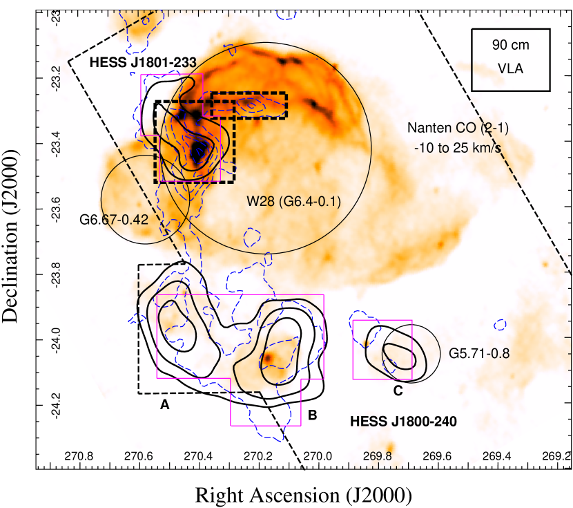
Figure 1: An image of 90 cm continuum emission (linear 0.06-0.55 Jy beam^-1) observed with the VLA (Brogan et al., 2006). TeV gamma-ray emission significance (3-6 $\sigma$) contours (thick, black) and CO (2-1) emission contours (dashed, blue) are overlaid (Aharonian et al., 2008b; Fukui et al., 2008).The approximate boundaries of catalogued SNRs (Brogan et al., 2006; Yusef-Zadeh et al., 2000) are displayed as black thin circles.Regions from previous 12 mm mapping campaigns (including HOPS data from Walsh et al. 2008) are enclosed by a thin black dashed boundary, whereas thin, solid magenta boundaries indicated previous 7 mm mapping regions. Thick dashed black boxes indicate the mapped regions in this work.

2 Mopra Observations and Data Reduction

The observations were performed with the Mopra radio telescope in April of 2010. We have also included the earlier observations from the 2008 and 2009 seasons (Nicholas et al., 2011), as well as data from the H₂O Southern Galactic Plane survey (Walsh et al., 2008) where possible (see Figure 1). Raw data are available from the Australia Telescope National Facility data archive under the project code M519 and data products are published online. All of these observations have utilised the UNSW Mopra wide-band spectrometer (MOPS) in zoom mode. Mopra is a 22 m single-dish radio telescope located $\sim$450 km northwest of Sydney, Australia ($31^{\circ}16^{\prime}04^{\prime\prime}$ S, $149^{\circ}05^{\prime}59^{\prime\prime}$ E, 866m a.s.l.). The 12 mm receiver operates in the 16-27.5 GHz frequency range. The spectrometer, MOPS, allows an instantaneous 8 GHz bandwidth. MOPS can record 16 different 137.5 MHz-wide windows simultaneously when in ‘zoom’-mode. Each of these 16 windows contains 4096 channels in each of two polarisations. At 12 mm this gives MOPS an effective bandwidth of $\sim$1800 km s^-1 with a resolution of $\sim$0.4 km s^-1. Across the whole 12 mm band, the beam FWHM varies from 2.4^′ (19 GHz) to 1.7^′ (27 GHz) (Urquhart et al., 2010).

We use the MOPS frequency band set-up outlined in Nicholas et al. (2011) to target the TeV source HESS J1801$-$233. We completed an additional thirty two passes towards the NE cloud, building on the previous four passes from 2008 and 2009 (making a total of 36 passes). The scanning direction was alternated between right ascension-aligned and declination-aligned to reduce the incidence of scanning artefacts.

In addition to the HESS J1801$-$233 field, two new passes were carried out towards a second shocked cloud north of W28 also containing a cluster of 1720 MHz OH masers (see Figure 1), but these yielded no new detections (see north-west maser clump in Figure 2), so are not addressed directly in this report.

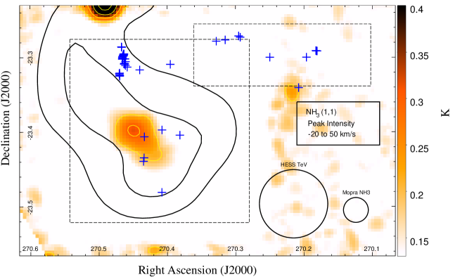
Figure 2: Peak NH₃ (1,1) intensity map of the 2 regions (black dashed boxes) in this study. Thick black contours represent the H.E.S.S. TeV statistical significance (4 and 5 $\sigma$ levels) and yellow contours represent NH₃ (1,1) intensity (T${}_{A}^{*}$) in increments of 0.1 K starting from 0.2 K. OH masers are represented by blue crosses. The exposure time varies over across the displayed field.

Data were reduced using the standard ATNF packages Livedata, Gridzilla (Gooch, 1996) and Miriad (Saul et al., 1995). For mapping data, Livedata was used to perform a bandpass calibration for each row, using the preceding off-scan as a reference, and apply a linear fit to the baseline. Gridzilla re-gridded and combined all data from all mapping scans into a single data cube, with pixels ($\Delta\,x,\Delta\,y,\Delta\,z$)=(15^′′, 15^′′, 0.4 km s^-1). The mapping data were also T_SYS-weighted, smoothed with a Gaussian of FWHM equal to the Mopra beam (2^′) and a cut-off radius of 5^′.

The antenna temperature, T${}_{\rm A}^{*}$, (corrected for atmospheric attenuation and rearward loss) was converted to the main beam brightness temperature, T_mb = T${}_{\rm A}^{*}$/$\eta_{\rm xb}$ where $\eta_{\rm xb}$ is the Mopra extended beam efficiency, which ranged from 0.68 to 0.74 for the NH₃ bands (Urquhart et al., 2010).

Across the bandpass, the standard deviation in T_xb achieved from these mapping observations is $\sim$0.03 K channel^-1.

Images of velocity-integrated intensity, position velocity (PV) and velocity dispersion, $v_{\rm RMS}$, were produced using Miriad software. In integrated emission images, minimum contour levels were set based on the integrated significance of the emission, which was determined on an image by image basis.

Velocity dispersion (Miriad moment 2), $v_{\rm RMS}$, maps were calculated for pixels above a reasonable threshold ($\sim 3.5$ T_RMS) using the same method as (Nicholas et al., 2011, Section 4.3).

3 Analysis and Results Overview

The primary targets of the survey were the NH₃(1,1) to (4,4), (6,6) and (9,9) transitions, with the goal of determining the location of hot, dense molecular gas. The spectrometer (MOPS) was also tuned to receive the NH₃(2-1), (3-2), (4-1), (7-5), (8-6), (9-7) and (11-9) transitions (see Nicholas et al. 2012 for line frequencies). Previously, the NH₃ (1,1), (2,2), (3,3) and (6,6) transitions were detected from the NE cloud. This recent survey has recorded the NH₃(4,4) inversion transition, in addition to these. We note that the (5,5) transition was not included in the spectrometer sampling range.

In addition to the NH₃ transitions, a 22 GHz H₂O maser was detected, but other spectral lines included within the MOPS bandpass, including class II CH₃OH masers, HC₃N(3-2) and the recombination lines H65 $\alpha$ and H69 $\alpha$, were not detected

Integrated intensity maps of detected NH₃ transitions are presented in Figure 4. The peak of the NH₃ velocity-integrated emission is positionally consistent for the five detected inversion transitions. The NH₃ features highlighted in Nicholas et al. (2011) are consistent with those in these new images, but now, our deeper mapping reveals weaker features which were not previously seen (at a significant level).

We detect a larger dense component of the NE cloud ($270.45^{\circ},-23.4^{\circ}$), including an extension of the dense gas protruding south in all detected NH₃ transitions, following the general distribution of the gas seen by the Nanten telescope in CO(2-1) emission (Nicholas et al., 2011), as seen in Figure 3 (Fukui et al., 2008). This NH₃ emission region is also coincident with CS(1-0) emission seen by Nicholas et al. (2012) and it follows that a significant proportion of the NE cloud is composed of dense, $\sim 10^{4}$ cm^-3 gas or higher (i.e. similar to the critical density for NH₃(1,1) emission).

An additional dense clump separated from the main NH₃ cloud is detected at an integrated intensity equivalent to a 3 to 4 $\sigma$ level ($270.30^{\circ},-23.48^{\circ}$) in the NH₃ (1,1) to (4,4) inversion transitions (Figure 4). It lies to the south west, outside the 3 $\sigma$ TeV contour, at a different velocity (V_LSR $\sim$15 km s^-1) to that of the majority of the dense gas mass in the region (V_LSR $\sim$7 km s^-1), as evidenced in Figure 5.

‘Postage stamp plots’ for the detected NH₃ lines are presented in Figure 5. In this figure, the background integrated intensity images are the same as presented in Figure 4, but with a modified colour scale (now white displays stronger emission) and fewer contour levels (now cyan). The mapped area is divided into a 6$\times$6 grid and the average line profile from all pixels within that grid box is displayed. These postage stamp plots display additional trends for the NH₃ line emission across the dense cloud component. Generally, the line profiles are broader towards the W28 side of cloud (south-west side of Figure 5). Here, the line profiles indicate the shocked cloud structure with broad line widths (FWHM $>$ 10 km s^-1) and blending of the NH₃ (1,1) satellite components. Additionally, a strong detection of NH₃ (3,3) ($270.39^{\circ},-23.43^{\circ}$), with a peak intensity $\sim 2\times$ larger than the NH₃ (1,1) line, and peaks in the NH₃(4,4) and (6,6) lines are seen towards the W28 side (south-west) of the cloud. Further west, towards W28, the line profiles are broad and weak, indicating that a shock may be coming from this direction. Towards the NE of the dense cloud, the line profiles are more ‘typical’ of a cold quiescent cloud. The characteristic satellite lines of NH₃ (1,1) are resolved and the peak intensity of the emission decreases in the higher-excited (2,2) and (3,3) states of NH₃.

The distribution of the NH₃ (1,1) and SiO (1-0) emission from the NE cloud is displayed in Figure 3, revealing the position and extent of the shocked and disrupted gas in the dense cloud component. In addition to intense SiO(1-0) emission coincident with the NH₃ (1,1) peak, SiO(1-0) was detected towards the northern OH maser clusters (see Nicholas et al., 2012, for details), coincident with the boundary between the shocked and quiescent gas, as indicated by CO emissions (Arikawa et al., 1999). This subregion also corresponds to a brightening of the X-ray shell in the 1-10 keV energy band (Ueno et al., 2003; Nicholas et al., 2012). As can be seen from Figures 4 and 5, emission from NH₃ (1,1) to (4,4) is seen here, and the broadness (6-13 km s^-1) of the NH₃ (3,3) and (4,4) spectral lines indicate the presence of gas with high temperature and disruption, in agreement with indications from the previous shocked gas tracers (SiO, OH).

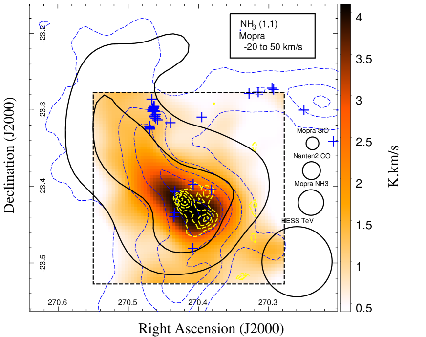
Figure 3: NH₃ (1,1) integrated intensity emission image (-20 to 50 km s^-1) with H.E.S.S. TeV significance contours (thick solid black, 4 and 5 $\sigma$ levels), SiO (1-0) integrated emission contours (yellow dashed, $\sim$2 to 5 $\sigma$ levels) from Nicholas et al. 2012 and Nanten2 CO(2-1) integrated emission contours (blue dashed). Positions of 1720 MHz OH masers from Frail et al. (1994); Claussen et al. (1997) are indicated by the blue crosses ($+$).

Figure 4: Integrated NH₃ emission intensity images (T_mb) towards the NE cloud. HESS TeV gamma-ray emission is indicated by thick, black contours (4 and 5 $\sigma$ levels). The black dashed box illustrates the region of deep mapping (this campaign). The blue crosses ($+$) indicate the positions of the 1720 MHz OH masers (Claussen et al., 1997). Yellow contours are used to show significant emission from each map. The minimum contour level on all images is 3 $\sigma$ and increments are in +2 $\sigma$ levels. The minimum contour levels are 0.51 K km s^-1 for NH₃ (1,1), 0.51 K km s^-1 for NH₃ (2,2), 0.45 K km s^-1 for NH₃ (3,3), 0.42 K km s^-1 for NH₃(4,4) and 0.3 K km s^-1 for NH₃(6,6). The integration velocity-range is larger for NH₃(1,1) emission to encompass prominent satellite emission lines. All images have been corrected for beam efficiency.

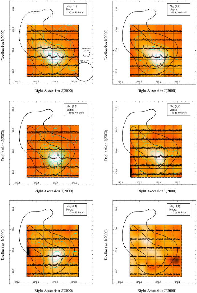
Figure 5: Postage stamp plot of the NH₃ emission lines towards the NE cloud of W28. The colour integrated-intensity images represent the same data as in Figure 4, but with modified colour scale and fewer contour levels (cyan). The average molecular line profile for all pixels within that grid box is provided. The spectral grid limits are the same for all 36 spectra within each emission line image. The velocity axes limits are $-$50 to 50 km s^-1. A red dashed line indicates the zero line. For all spectral panels the ordinate lower limit is $-$0.1 K, whereas the ordinate upper limits are 0.3, 0.3, 0.4, 0.2, 0.2, 0.2 K for NH₃ (1,1), NH₃ (2,2), NH₃ (3,3), NH₃(4,4), NH₃(6,6) and NH₃(9,9), respectively. HESS TeV gamma-ray emission is indicated by thick, black contours (4 and 5 $\sigma$ levels).

3.1 Velocity Dispersion

Previously, Nicholas et al. (2011) used a velocity dispersion profile map to illustrate that the western side of NE cloud was experiencing greater disruption than the east. Additionally, the greatest level of dispersion, in both physical area and magnitude, was seen in the NH₃ (3,3) line.

Figure 6 presents four velocity dispersion (intensity-weighted FWHM, see moment 2 in Saul et al. 1995) images generated using our sensitive NH₃ transition data. This series of images has similar features to those in Nicholas et al. (2011), although one new structure is observed. The deeper NH₃ (1,1) data now reveals two peaks or a long finger of broad gas in the dispersion map (compared to only one in Nicholas et al. 2011). One peak is towards the centre-east of the cloud core ([$\alpha$,$\delta$]$\sim$[270.44,-23.42]), which was previously observed, whereas a second, slightly stronger peak is detected towards the western side of the cloud([$\alpha$,$\delta$]$\sim$[270.37,-23.42]). The former peak in (1,1) velocity dispersion also appears to correspond to an eastern extension in the (4,4) dispersion image.

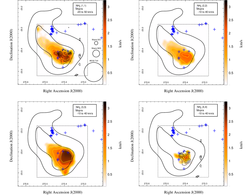
Figure 6: Velocity dispersion, $v_{\rm RMS}$ (km s^-1), maps for the NE cloud. These images are the updated equivalents from Nicholas et al. (2011, Figure 9). In all panels thick black contours are the H.E.S.S. TeV statistical significance (4 and 5 $\sigma$ levels) and OH masers are represented by blue crosses. The NH₃ (1,1), NH₃ (2,2), NH₃ (3,3) and NH₃(4,4) dispersions are calculated for pixels with $\mbox{T${}_{\rm mb}$}\geq 3.5$ $\sigma$ ($\sim$0.11 K) within a V_LSR range of 5 to 15 km s^-1. In 2 images, black dashed contours represent SiO (1-0) emission integrated between V_LSR $=-$5 and 20 km s^-1 ($\sim$3 to 5 $\sigma$ levels, see Nicholas et al. 2012). We note that the largest region of dispersion is apparent in the NH₃ (3,3) line.

We note that Nicholas et al. (2012) showed shock-tracing SiO(1-0) emission towards the western side of the cloud, but this new NH₃(1,1) velocity dispersion peak lies even further west, as illustrated in Figure 6. Furthermore, the peak of NH₃(4,4) velocity dispersion appears spatially better-matched to the SiO(1-0) emission (with a FWHM a factor 2 less than that of NH3(1,1) emission), suggesting that this is the most disturbed part of the cloud. Six 1720 MHz OH masers lie around the periphery of this region, suggesting that conditions conducive to the generation of 1720 MHz OH masers directed towards the Earth are not present in the densest, most-energetic region of the north-east cloud, but are instead offset from the position of peak NH₃(4,4) emission.

Another indication of a disruption occurring from the south-west side of the cloud can be seen in images of peak intensity ratios in Figure 7. The raw values of these images are a product of several inter-related parameters, hence are difficult to directly interpret. The gradients in these images indicate a general trend towards a greater intensity of higher-energy inversion transitions towards the south-west compared to NH₃(1,1). This trend is particularly prominent for the NH₃(3,3) inversion line, unclear from the NH₃(6,6) and less prominent for the NH₃(2,2) and (4,4) lines. On examining the NH₃(3,3)/NH₃(1,1) gradient, it is clear that a temperature gradient is present, although we can’t immediately discount the possibility of effects caused by differences in ortho and para-NH₃ abundances in a shocked/energetic region (e.g. Umemoto et al. 1999). This issue is considered in Section 3.3. Certainly the NH₃(3,3) emission does exhibit another unique feature - a southern lobe present in the (3,3) dispersion image (Figure 6), but not in the (1,1) or (2,2) images. This extension is also seen in CO(3-2) emission (Arikawa et al., 1999), so a hot component may be seen to extend towards this same location.

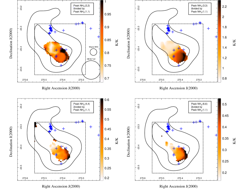
Figure 7: Images of the peak intensity of NH₃(n,n) emission divided by the peak intensity of NH₃(1,1) emission, where n=2,3,4 and 6. All non-zero pixels had both the constituent peak intensity pixel values exceed a threshold chosen by eye - 0.15, 0.15, 0.13, 0.08 and 0.07 K for the (1,1), (2,2), (3,3), (4,4) and (6,6) transitions, respectively. OH masers are represented by blue crosses.

3.2 LTE Parameter Calculation Prescription

The greater sensitivity achieved from deep 12 mm mapping has allowed us to parametrise the NH₃ satellite lines on a pixel-by-pixel (PbP) basis. An NH₃ analysis could thus be performed on arcminute scales. This includes the calculation of NH₃ (1,1) main line optical depth (Barrett et al., 1977, Equation 2), NH₃ energetic state column densities (Goldsmith & Langer, 1999, Equation 9), the rotation temperature (via rotation diagrams) and the total NH₃ column density. A summary of the formulae employed can be found in section B1 of Maxted et al. (2012), but the method presented here is adjusted to account for higher temperatures.

Our PbP procedure considered each pixel in the NH₃ (1,1), (2,2), (3,3), (4,4) and (6,6) data cubes separately, and does not attempt to use low signal-noise NH₃(9,9) emission. Five Gaussian functions were fitted to the 5 satellite components of NH₃ (1,1) emission, and pixels that had a peak main line intensity $\leq 0.13$ K ($\sim 4$ T_RMS) were discarded (set equal to zero). This threshold was decided after the examination of a sample of spectral fits, ensuring that only high-quality spectral parameters were used in our analyses. The optical depth was calculated, and the NH₃ (2,2) spectra were fit by single Gaussian functions (satellite lines were generally not resolved for NH₃ (2,2) emission). The NH₃ (1,1), (2,2), (3,3), (4,4) and (6,6) column densities (Goldsmith & Langer, 1999) were then calculated for all pixels with an integrated emission threshold above 0.5 K.km.s^-1 ($\sim$3 $\sigma$). Emission from energetic states (J,K)$=$(3,3) and above were assumed to be optically thin.

Rotation temperatures $T_{12}$ and $T_{36}$ were calculated using a line of best fit for degeneracy-normalised column density versus transition temperature (e.g. Umemoto et al. 1999), where the subscripts refer to the rotational quantum numbers (J) of the inversion transitions used to derive the temperature. Figure 8 illustrates the difference between the two rotational temperatures attributable to a pixel that is representative of the region with detections of all measured NH₃ lines. We attribute this to the existence of ‘cold’ and ‘hot’ components, with the (1,1) and (2,2) transitions being dominated by the more extensive cold component. The region where NH₃(6,6), (4,4) and (3,3) emission was observed was treated as a hot component and the ortho-para-ratio was calculated by finding the ratio between the observed NH₃(4,4) column density and that inferred from a trend line between the points corresponding to the (3,3) and (6,6) on the rotational diagram. In doing this, we interpolate that $T_{45}=T_{36}$, which is a valid assumption if all the NH₃(3,3)-(6,6) emission originates from the same region. Cold and hot component column densities were calculated using the NH₃ partition function (see Nicholas et al., 2011) assuming temperatures of $T_{12}$ and $T_{36}$, respectively. The calculated OPR was applied in the hot component analysis, but was assumed to be unity for the cold component where the calculation of an OPR was not possible.

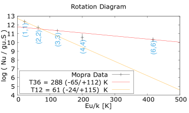
Figure 8: An example of a rotational diagram of NH₃ inversion transition data towards a pixel representative of the regions with detectable NH₃ (1,1), (2,2), (3,3), (4,4) and (5,5) lines. The y-axis is the column density divided by the statistical weight ($g_{u}$ is rotational degeneracy and $S$ is the spin degeneracy), and the x-axis is the measured NH₃ inversion transition energy in kelvin. Two best-fit linear lines are displayed, representing the cold component LTE rotational temperature (orange) and the hot component LTE rotational temperature (red), respectively.

The final results were assembled into 2D arrays of optical depths, temperatures and column densities, which were converted into fits files. Fits-file ‘header’ information was copied from the input NH₃ (1,1) fits cube to recreate the axes of the output fits files. The resultant parameter maps are displayed in Figures 9 and 10.

3.3 Gas Parameters towards HESS J1801$-$233

Five images are shown in Figure 9: NH₃ (1,1) main line optical depth, NH₃ (2,2) optical depth, the NH₃(3,3)/NH₃(6,6) rotational temperature and the estimated ortho to para-NH₃ ratio (OPR). Figure 10 displays the column densities of the (1,1), (2,2), (3,3), (4,4), (6,6) NH₃ states, and the total hot + cold component NH₃ column density calculated from the method outlined in Section 3.2. In all images, a lower threshold was imposed to ensure the quality of results (see Section 3.2), thus pixels with a value of zero do not represent a value of zero but rather an undefined value.

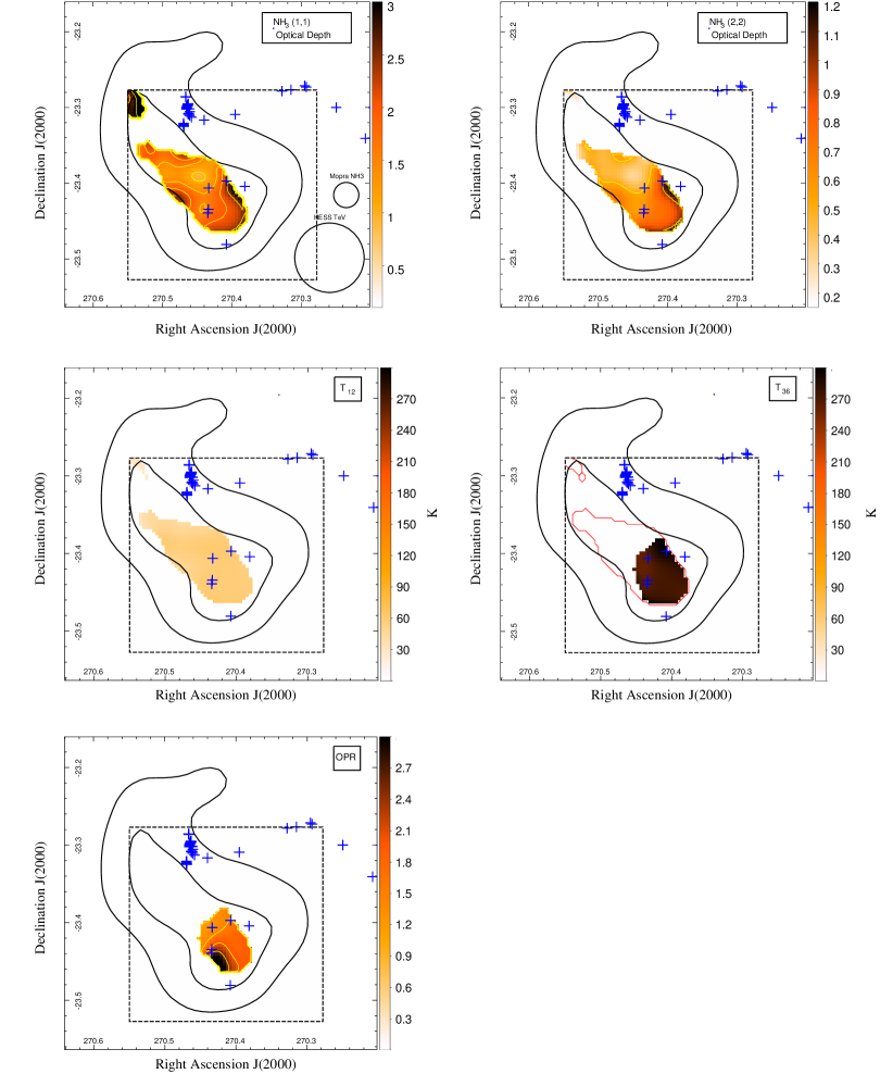
Figure 9: Images of NH₃(1,1) and (2,2) optical depth (top left and right, respectively), the NH₃(1,1)/NH₃(2,2) rotational temperature, T₁₂(middle left), NH₃(3,3)/NH₃(6,6) rotational temperature, T₃₆(middle right), and the ortho-para-NH₃ ratio, the OPR (bottom right). Optical depth images have contours in increments of 0.5 from 0. The ortho-para ratio map (OPR, bottom, right) has contours of 1 to 2.5 in increments of 0.5. OH masers are represented by blue (or white, where necessary) crosses in all maps. Maps of the error associated with all of these values are displayed in Figure 11.

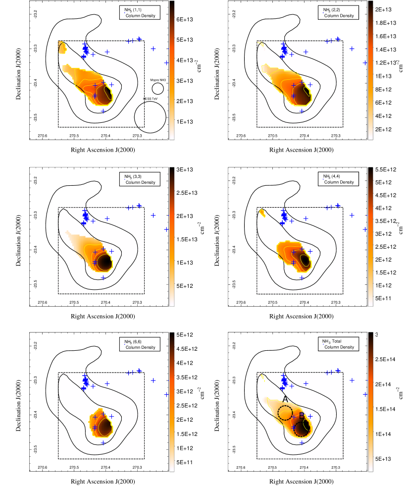
Figure 10: Column densities of the (1,1), (2,2), (3,3), (4,4), (6,6) NH₃ states and the total NH₃ column density. The total NH₃ column density image has been additionally smoothed by a 2D gaussian function with width equal to the Mopra NH₃(1,1) beam width, and contains 2 circular regions which were exploited for non-LTE cross-checks (see Section 3.3.2). OH masers are represented by blue crosses. NH₃(1,1) and total column density error maps are displayed in Figure 11 and 12, respectively.

3.3.1 Optical Depth

The NH₃(1,1) optical depth map (Figure 9) reveals an optically thick ($\tau\sim$0.9-3) region corresponding to the peak of NH₃ (1,1) emission (Figure 4). Some variation is observed on a scale larger than the Mopra NH₃(1,1) beam and this may reflect internal clumpiness in the dense gas. At declination$\sim\,-23.38^{\circ}$, a region of NH₃(1,1) optical depth, $\tau\sim$1, transitions into a region of NH₃(1,1) optical depth, $\tau\sim$2, towards the southern part of the cloud at declination$\sim-23.45^{\circ}$. Towards the edges are some regions with optical depths which tend towards $\tau\sim$3. These features are smaller than the NH₃(1,1) beam and possibly artefacts introduced by the gaussian function fitting process, when the main emission line intensity becomes more comparable to noise. Towards the western side of the dense cloud (as seen in the integrated NH3 (1,1) emission image, Figure 4), where NH3 (1,1) profiles become broad and the satellite lines blend, optical depths could not be calculated as the sensitivity was not sufficient.

We note the existence of a relatively optically thick (optical depth $\tau\sim$3$\pm$1) gas component in the north-east corner of the map (Figure 9, top left). Upon examination of the corresponding NH₃ (1,1) spectra (see Figure 5), this feature appears to be from a real emission line, but we cannot rule out the high optical depth value being an artefact of the analysis. The flux falls below the threshold limit around this region, so the extent of the feature cannot be determined. On examination of the corresponding NH₃(2,2) optical depth map (Figure 9), the feature is present with an optical depth of $\sim$0.2, otherwise the (2,2) optical depth is generally 30-50% of that of the (1,1) optical depth throughout the main cloud component, where the (2,2) optical depth follows the same general trend as the (1,1) optical depth.

3.3.2 Temperature and the ortho-para-NH₃ ratio

Figure 10 displays the column densities of the (1,1), (2,2), (3,3), (4,4), (6,6) NH₃ states and the total NH₃ column density. The column density of each rotational state and the total NH₃ column density peaks towards the south-west region of the cloud and decreases steadily towards the north-east. This column density gradient may indicate a region of dense gas or shock-compression triggered by the W28 SNR, a scenario consistent with the detection of higher-energetic state NH₃ transitions.

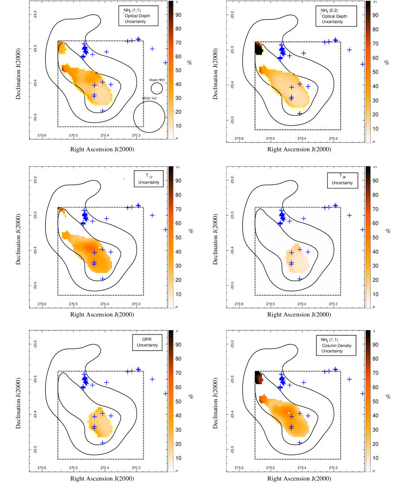
Figure 11: Images of the uncertainty in NH₃(1,1) and (2,2) optical depth (top left and right, respectively), rotational temperatures (middle, left and right), the OPR (bottom left) and NH₃(1,1) column density (bottom, right). OH masers are represented by blue crosses in all maps.

Towards the main cloud dense component, the calculated rotational temperatures (see Figure 9) were relatively spatially constant ($T_{12}\sim$40-60$\pm$(10-40) K and T${}_{36}\sim$260-295$\pm$(20-65) K). A non-LTE statistical equilibrium anlaysis of the same data (see below) yields a kinetic temperature consisitent with T₁₂, disfavouring T₃₆ as reliable measure of kinetic temperature. Within uncertainties, no spatial rotational temperature gradient is observed within either single rotational temperature map. The typical uncertainty was 10-20% for T₃₆, but 30-60% for T₁₂ towards the cloud. These errors lead to a hot component LTE column density with an error of 3-10% and a cold component LTE column density with an error of 25-70% (disregarding results for the component at the north-east corner, which has an error exceeding 100%). After adding hot and cold components, the total column density had an error in the range 30-75%. Percentage uncertainty maps for 7 key parameters calculated in this analysis are shown in Figure 11 and 12.

The ortho-para-NH₃ ratio (see Figure 9) was observed to vary between 1 and 3.4, with a statistical uncertainty of $\sim$18-40%. A high OPR ($>$2) is thought to indicate that the observed NH₃ originally formed on the surface of dust grains before being freed by heat or shock-collisions (Umemoto et al., 1999). Upcoming work by de Wilt et al. (2015 in prep.) will focus on NH₃ emission and the OPR values towards a population of gamma-ray sources, including W28-north, so we leave further investigation of this phenomenon as future work.

We performed non-LTE statistical equilibrium modelling to test the validity of our LTE analysis for 2 test regions, A and B, within the W28 NE cloud (see Figure 10). The RADEX statistical modeling software (van der Tak et al., 2007) was employed to cycle through density and temperature parameter spaces to retrieve the best-fit (single component) values consistent with measured NH₃ inversion line observations via a $\chi^{2}$-minimisation method. Parameter solutions were found for ortho and para-NH₃ emission lines in joint (ortho$+$para lines) analyses, using observed column density constraints, line intensities and NH₃(1,1) optical depths as inputs. An OPR of 2.3$\pm$0.5 was imposed for Region B, consistent with observations, but the OPR was assumed to be unity for Region A, where the OPR could not be calculated. The density-space between $10$ cm^-3 and $10^{10}$ cm^-3, and the temperature-space between 10 and 400 K were tested. Molecular H₂ was assumed to be the only collision partner in our simulations.

NH₃ non-LTE analyses yielded temperature solutions consistent with T₁₂ in a $\chi^{2}$ minimisation process for both Regions A and B, with temperatures of $\sim$55-70 and $\sim$35 K, respectively. These analyses also suggest that the emitting clumps within Region A have a density of $\sim 2\times 10^{5}$-$2\times 10^{6}$ cm^-3. Non-LTE analyses also yielded a degenerate solution for the density of Region B of $\sim 10^{4}$ and $>10^{8}$ cm^-3, perhaps demonstrating a limit of single-component non-LTE modelling for this region. The former solution is the approximate critical density of NH₃(1,1), so is consiedered to be the most likely solution for Region B. This density information is revisited in the following section.

3.4 Column density, Filling Factor and NH₃ Abundance

In Nicholas et al. (2011), the dense gas component of the NE cloud was investigated using NH₃ (1,1) emission data less sensitive to those used here. The mass and density were calculated to be 1600 M_⊙ and $\sim 800$ cm^-3 respectively, and further radiative transfer modelling with MOLLIE software suggested that the NE cloud had a mass $>1300$ M_⊙, however this value was calculated under the assumption that [NH₃]/[H₂]$\sim 2\times 10^{-8}$. In this paper, the variation in Galactic NH₃ abundance is considered instead, and the reverse process is employed, i.e. a mass is used to calculate the abundance of Ammonia in the W28 NE cloud.

Observations of the CS(1-0) transition, which has a similar critical density to NH₃(1,1), found that the mass of the dense gas component of the NE cloud is $\sim$5.6$\times 10^{4}$ M_⊙ (Nicholas et al., 2012), in agreement with previous CO-derived mass estimates (Aharonian et al., 2008b). CS(1-0) emission covers a region 30% larger than the area that passed the quality checks in this NH₃ analysis. The average CS-derived H₂ column density towards the NH₃-traced region highlighted in Figures 9-10 is $\sim$10²³ cm^-2. This value is supported by the implied optical extinction of $\sim$50 (e.g. Guver & Ozel, 2009), which is consistent with the extinction value of 57 derived from infrared emission using a visual extinction to reddening ratio of 3.1 (Schlafly & Finkbeiner, 2011). The average NH₃ column density within the region is (1.5$\pm$0.6)$\times$10¹⁴ cm^-2, leading to an estimated NH₃ abundance of [NH₃]/[H₂]$\sim(1.2\pm 0.5)\times 10^{-9}$.

NH₃ abundance is observed to vary in different Galactic environments, with NH₃ molecules being released from dust-grains in warm environments, while being vulnerable to photo-dissociation in ionising UV and CR radiation fields. Typical NH₃ abundance values inside infrared-dark clouds are of the order 10^-8 (Flower et al., 2004; Stahler & Palla, 2005; Rizzo et al., 2014), with hot ($>$100 K) regions sublimating enough NH₃ from dust grain mantles (e.g Tafalla et al. 2004) to make the gas-phase abundance increase, sometimes as high as $\sim$10^-6 (Osorio et al., 2009). Such behaviour is also observed towards some shocks to various levels, e.g. [NH₃]/[H₂]$\sim$10^-6 in the bipolar outflow L1152 (Tafalla et al., 1995) and $\sim$10^-8 in the Wolf-Rayet nebula NGC 2359 (Rizzo et al., 2001). Photo-dissociation can have the opposite effect on NH₃ abundance, like near the intense UV field of the luminous blue variable star G79.29+0.476 (Rizzo et al., 2014). Cosmic ray (CR) dissociation can also play a role according to modelling of the chemistry in CR-dominated regions, with ionisation rates above 10^-16 s^-1 resulting in a significant decrease in NH₃ abundance (Bayet et al., 2011). Although the average ionisation rate inside dense clouds might be as low as 10^-18-10^-17 s^-1 (e.g. Padovani et al., 2014), direct measurements in the far north of the NE cloud suggest ionisation rates on the order of 10^-15 s^-1 (Vaupre et al., 2014).

The W28 NE cloud is likely a clumpy region and this can be investigated by by estimating the filling factor, $f$. By assuming a spherical clump of density, $n_{H2}$, and line-of-sight thickness, $L$, within the Mopra beam area, the column density can be expressed as $N_{H2}=f.n_{H2}.L$. The filling factor in this case would be the ratio of the cross-sectional area of the emitting clump, $\pi.(L/2)^{2}$, and the beam area, $\pi.(D/2)^{2}$, leading to $f=\left(L/D\right)^{2}$. Combining the column density and filling factor equations then allows an estimation of the filling factor,

$$f=\left(\frac{N_{H2}}{n_{H2}.D}\right)^{\frac{2}{3}}~{}=~{}\left(\frac{N_{NH3}}{\chi.n_{H2}.D}\right)^{\frac{2}{3}}$$ (1)

where $\chi$ is the NH₃ abundance with respect to molecular hydrogen. D$\sim$1.2 pc corresponds to the Mopra beam FWHM at 2 kpc. From the non-LTE analyses, Regions A and B were estimated to have densities of $\sim 2\times 10^{5}$-$2\times 10^{6}$ and $\sim 10^{4}$ cm^-3, respectively (see Section 3.3.2). Inserting these values into Equation 1 yields filling factors of $\sim 0.05$-$0.25$ and $\sim$2 for Regions A and B, respectively These estimates suggest that emitting NH$3$ clumps are distributed on scales from 0.2^′ to scales comparable to the beam FWHM (2^′). Interferometric NH₃ observations of finer angular resolution may be able to resolve such structure within the Mopra beam. Indeed, SiO(1-0) observations already show features on a 1^′-scales (see Figure 3 and Nicholas et al. 2012).

Given the complexity of this region, the estimated NH₃ abundance of $(1.2\pm 0.5)\times 10^{-9}$ from the LTE analysis presented in this paper may be the result of a balancing between NH₃-release from dust grains and NH₃-destruction pathways resulting from radiation and CRs. An elevated OPR, like that observed in Region B, suggests that NH₃ has been released from dust grains (Umemoto et al., 1999). On the other hand, there is no indication that an accompanying NH₃ abundance increase has occurred. In fact, the NH₃ abundance may be an order of magnitude below that of a typical infrared-dark cloud, despite the high temperature and shocked environment (see Section 3.1). This low abundance may suggest that an NH₃ destruction mechanism is playing a significant role. Through this line of reasoning, a high-OPR/low-abundance combination may indeed be another piece of evidence to show that the NE cloud is heavily influenced by the W28 SNR, both directly through shock collision and shock heating, and indirectly from an enhanced ionisation rate. Such a scenario would require modelling of gas-phase NH₃ production and destruction beyond the scope of this work. We note that in our calculations, the NH₃ abundance is proportional to the CS abundance assumed by Nicholas et al. (2012), thus an alternative interpretation for our data towards this cloud is that the CS abundance is enhanced by a factor of $\sim$10 in the region, while the NH₃ abundance remains average ($\sim 2\times 10^{-8}$). Certainly CS abundance can fluctuate due to freeze-out onto grains (e.g. Tafalla et al., 2004).

4 Summary, Conclusions and Future Work

We reported on deep mapping observations towards the shocked molecular cloud north-east of W28, with a focus on detecting multiple NH₃ inversion transitions. The NE cloud has a remarkable spatial match with the gamma-ray source HESS J1801-233, so constraints on the mass distribution are important for hadronic gamma-ray production models of the region, while the observed chemistry serves as an observational constraint on CR ionisation and propagation. Spectral line observations are steps towards parameter constraints associated with the NE cloud of W28.

These observations revealed that the dense component of the NE cloud is much more extended than previously reported. This is the case for all the detected inversion transitions. Towards the cloud, strong NH₃ (3,3), NH₃(4,4) and NH₃(6,6) emission suggest this is a region of high gas temperature. Furthermore, new evidence for shocked gas is provided by NH₃ (1,1)  -NH₃ (3,3) velocity dispersion maps that resolve a new NH₃ component on the W28 side of the NE cloud.

Gas parameter maps were derived from NH₃ emission via a method that assumes Local Thermodynamic Equilibrium (LTE) and were checked against non-LTE statistical equilibrium models. NH₃ column densities on the order of 10¹⁴ cm^-2 and temperatures in the range 35-60 K were observed within the NE cloud of W28.

The ortho-para-NH₃ ratio (OPR) was investigated, revealing a subregion with an elevated OPR ($>$2), characteristic of regions where NH₃ is liberated from dust-grain mantles. Comparing our measurements with a previously-published CS-derived mass estimate, no corresponding NH₃ abundance enhancement was observed ([NH₃ ]/[H₂]$\sim(1.2\pm 0.5)\times 10^{-9}$), possibly suggesting the existence of an NH₃ destruction mechanism. More detailed modelling of gas-phase NH₃ production and destruction may be required to investigate this result.

Future work to improve the angular resolution and sensitivity of TeV gamma-ray images will allow a detailed comparison of the gamma-ray emission and cosmic ray target material (the gas), while considering the time-dependent effect cosmic ray propagation may also allow the analysis of features in the GeV to TeV gamma-ray spectrum towards SNRs (e.g. Gabici & Aharonian, 2007; Maxted et al., 2012).

Appendix A Uncertainties of key parameters

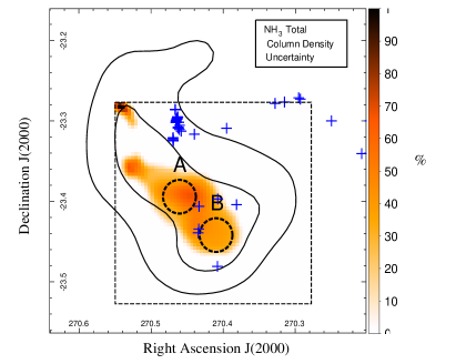
Figure 12: Image of the uncertainty of the total NH₃ column density. OH masers are represented by blue crosses and Regions A and B, which were used for non-LTE cross checks (see Section 3.3.2) are displayed.

References

- Abdo et al. (2010) Abdo A. A., et al. (Fermi Collab.), 2010, ApJ 718, 348
- Aharonian et al. (2008b) Aharonian F., et al. (H.E.S.S. Collab.), 2008b, A&A, 481, 401
- Arikawa et al. (1999) Arikawa Y., Tatematsu K., Sekimoto Y. & Takahashi T., 1999, PASJ, 51, L7
- Barrett et al. (1977) Barrett A. H., Ho P. T. P. & Myers P. C., 1977, ApJ, 211, L39
- Bayet et al. (2011) Bayet E., Williams D. A., Hartquist T. W. & Viti S., 2011, MNRAS, 414, 1583
- Becker et al. (2011) Becker J. K., Black J. H., Safarzadeh M. & Schuppan F., 2011, ApJ, 739, L43
- Brogan et al. (2006) Brogan C. L., Gelfand J. D., Gaensler B. M., Kassim N. E. & Lazio T. J. W., 2006, ApJ, 639, L25
- Claussen et al. (1997) Claussen M. J., Frail D. A., Goss W. M. & Gaume R. A., 1997, ApJ, 489, 143
- DeNoyer et al. (1983) DeNoyer L. K., 1983, ApJ, 264, 141
- Dubner et al. (2000) Dubner G. M., Velázquez P. F., Goss W. M., Holdaway M. A., 2000, AJ, 120, 1933
- Faure et al. (2013) Faure, A., Hily-Blant, P., Le Gal, R., Rist, C., & Pineau des Forets G., 2013, 770, L2
- Schlafly & Finkbeiner (2011) Schlafly E. & Finkbeiner D., 2011, ApJ, 737, 103
- Flower et al. (2004) Flower D. R., Pineau des Forets G., and Walmsley C. M., A&A, 427, 887
- Frail et al. (1994) Frail D. A., Goss W. M. & Slysh V. I., 1994, ApJ, 424, L111
- Fukui et al. (2008) Fukui Y. et al. (Nanten Collab.), 2008, AIP Conf. Proc., 1085, 104
- Gabici & Aharonian (2007) Gabici, S. & Aharonian, F., 2007, Ap&SS, 309, 365
- Goldsmith & Langer (1999) Goldsmith, P. F. & Langer W. D., 1999, ApJ, 517, 209
- Gooch (1996) Gooch, R.E., 1996, PASA, 14, 106
- Goudis (1976) Goudis C., 1976, Ap&SS, 40, 91
- Giuliani et al. (2010) Giuliani A., et al. (AGILE Collab.), 2010, A&A 516, L11
- Guver & Ozel (2009) Guver T. & Ozel F., 2009, MNRAS, 400, 2050
- Hewitt & Yusef-Zadeh (2009) Hewitt J. W., Yusef-Zadeh F., 2009, ApJ, 694, L16
- Ho & Townes (1983) Ho P. T. P. & Townes C. H., ARA&A, 21, 239
- Kaspi et al. (1993) Kaspi V. M., Lyne A. G., Manchester R. N., Johnston S., D’Amico N. & Shemar S. L., 1993, ApJ, 409, L57
- Keto (1990) Keto E., 1990, ApJ, 355, 190
- Lozinskaya (1981) Lozinskaya T. A., 1981, Sov. Astron. Lett., 7, 17
- Maxted et al. (2012) Maxted, N., Rowell G., Dawson, B., Burton, M., Kawamura, A., Walsh, A., Sano, H., 2012, MNRAS, 422, 2230-2245
- Maxted et al. (2013a) Maxted, N., Rowell, G., Dawson, B., Burton, M., Kawamura, Fukui, Y., A., Walsh, A., Sano, H., et al., 2013a, MNRAS, 434, 2188
- Maxted et al. (2013b) Maxted, N., Rowell, G., Dawson, B., Burton, M., Fukui, Y., Lazendic, J., Kawamura, A., Horachi, H., et al., 2013b, PASA, 30, e055
- Motogi et al. (2010) Motogi K., Sorai K., Habe A., Honma M., Kobayashi H. & Sato K., 2011, PASJ, 63, 31
- Nakamura et al. (2014) Nakamura R., Bamba A., Ishida M., Yamazaki R., Tatematsu K., Kohri K., Puhlhofer G., Wagner S. J. & Sawada M., 2014, PASJ, 66, 62
- Nicholas et al. (2011) Nicholas B., Rowell G., Burton M. G., Walsh A., Fukui Y., Kawamura A., Longmore S. & Keto E., 2011, MNRAS, 411, 1367
- Nicholas et al. (2012) Nicholas B. P., Rowell G., Burton M. G., Walsh A. J., Fukui Y., Kawamura A., Maxted N. I. 2012, MNRAS, 419, 251-266
- Osorio et al. (2009) Osorio M., Anglada G., Lizano S. & D’Alessio P., 2009, ApJ, 694, 29
- Padovani et al. (2014) Padovani M., Hennebelle P. & Galli D., 2014, ASTRP, 1, 23
- Pihlstrom et al. (2014) Pihlstrom Y. M., Sjouwerman L. O., Frail D. A., Claussen M. J., Mesler R. A. & McEwen B. C., 2014, ApJ, 147, 73
- Reach et al. (2005) Reach W. T., Rho J., Jarrett T. H., 2005, ApJ 618, 297
- Rho & Borkowski (2002) Rho J. & Borkowski K. J., 2002, ApJ, 575, 201
- Rizzo et al. (2001) Rizzo J. R., Martin-Pintado J. & Henkel C., 2001, 553, L181
- Rizzo et al. (2014) Rizzo J. R., Palau A., Jimenez-Esteban F. & Henkel C., 2014, A&A 564, A21
- Rosolowsky et al. (2010) Rosolowsky E., Dunham M. K., Ginsburg A., Bradley E. T., Aguirre J., Bally J., Battersby C., Cyganowski C., et al., 2010, ApJSS, 188, 123
- Saul et al. (1995) Sault R.J., Teuben P.J., & Wright M.C.H., 1995, In Astronomical Data Analysis Software and Systems IV, ed. R. Shaw, H.E. Payne, J.J.E. Hayes, ASP Conference Series, 77, 433-436
- Schuppan et al. (2012) Schuppan F., Becker J. K., Black J. H. & Casanova S., A&A, 541, A126
- Stahler & Palla (2005) Stahler S. & Palla F., 2005, The Formation of Stars., Wiley, New York
- Tafalla et al. (1995) Tafalla M. & Bachiller R., 1995, ApJ, 443, 37
- Tafalla et al. (2004) Tafalla M., Myers P. C., Caselli P. & Walmsley C. M., 2004, A&A, 416, 191
- van der Tak et al. (2007) van der Tak F., Black J., Schoier F., Jansen D. & van Dishoeck E., 2007, A&A 468, 627-635
- Torres et al. (2003) Torres D. F., Romero G. E., Dame T. M., Combi J. A. & Butt Y. M., 2003, Phys. Rep. 382, 303
- Ueno et al. (2003) Ueno M., Bamba A. & Koyama K., 2003, proc. 28th ICRC, 2401
- Umemoto et al. (1999) Umemoto T., Mikami H., Yamamoto S. & Hirano N., 1999, ApJ, 525, L105
- Ungerechts et al. (1986) Ungerechts H., Walmsley C. M. & Winnewisser G., 1986, A&A, 157, 207
- Urquhart et al. (2010) Urquhart J. S., Hoare M. G., Purcell C. R., Brooks K. J., Voronkov M. A., Indermuehle B. T., Burton M. G., Tothill N. F. H. & Edwards P. G., 2010, PASA, 27, 321
- van der Tak et al. (2007) van der Tak F., Black J., Schoier F., Jansen D. & van Dishoeck E., 2007, A&A, 468, 627-635
- Vaupre et al. (2014) Vaupre S., Hily-Blant P., Ceccarelli C., Dubus G., Gabici S. & Montmerle T., 2014, A&A, 568, A50
- Walsh et al. (2008) Walsh A., Lo N., Burton M. G., White G. L., Purcell C. R., Longmore S. N., Phillips C. J. & Brooks K. J., 2008, PASA, 25, 105
- de Wilt et al. (2015 in prep.) de Wilt P., Rowell G., Walsh A., Burton M., Rathborne J., Fukui Y., Dawson B., Kawamura A., Aharonian F., Submitted(2016), MNRAS
- Walmsley & Ungerechts (1983) Walmsley C. M. & Ungerechts H., 1983 A&A, 122, 164
- Yusef-Zadeh et al. (2000) Yusef-Zadeh F., Shure M., Wardle M. & Kassim N., 2000, ApJ, 540, 842