Abstract

Motivated by holographic models of (pseudo)conformal Universe, we carry out complete analysis of linearized metric perturbations in the time-dependent two-brane setup of the Lykken-Randall type. We present the equations of motion for the scalar, vector and tensor perturbations and identify light modes in the spectrum, which are scalar radion and transverse-traceless graviton. We show that there are no other modes in the discrete part of the spectrum. We pay special attention to properties of light modes and show, in particular, that the radion has red power spectrum at late times, as anticipated on holographic grounds. Unlike the graviton, the radion survives in the single-brane limit, when one of the branes is sent to the adS boundary. These properties imply that potentially observable features characteristic of the 4d (pseudo)conformal cosmology, such as statistical anisotropy and specific shapes of non-Gaussianity, are inherent also in holographic conformal models as well as in brane world inflation.

1 Introduction

Some time ago it has been pointed out that conformal symmetry $SO(4,2)$ broken down to de Sitter $SO(4,1)$ in the early Universe may be responsible for the generation of the (nearly) flat spectrum of scalar cosmological perturbations [1, 2, 3, 4] (see Ref. [5] for a review). The main ingredient of the (pseudo)conformal scenarios is the expectation value of a scalar operator $\mathcal{O}$ of non-zero conformal weight $\triangle$ which depends on time $\tau$ and gives rise to symmetry breaking,

$$\langle\mathcal{O}\rangle\propto\frac{1}{(-\tau)^{\triangle}}\,,$$ (1)

where $\tau<0$. It is assumed also that: (i) space-time is effectively Minkowskian during the rolling stage (1); (ii) there is another scalar field of zero effective conformal weight in this background, whose perturbations automatically have flat power spectrum; (iii) the perturbations of the latter field are converted into the adiabatic scalar perturbations at some later stage.

A peculiarity inherent in the (pseudo)conformal mechanism is that the perturbations of $\mathcal{O}$ have red power spectrum,

$$\mathcal{P}_{\delta\mathcal{O}}\propto p^{-2}\;.$$ (2)

This feature leads to potentially observable predictions, such as specific shapes of non-Gaussianity [7, 8, 9] and statistical anisotropy [7, 8, 10, 11]. It is worth emphasizing that many of these properties are direct consequences of the symmetry breaking pattern $SO(4,2)\to SO(4,1)$ [8, 12].

Further development of the (pseudo)conformal scenario involves holography. It has been pointed out that conformal rolling (1) in the boundary theory is dual to motion of a domain wall in the adS₅ background [13, 14]. This motion corresponds to spatially homogeneous transition from a false vacuum to a true one. One generalizes this construction further and considers nucleation and subsequent growth, in adS₅, of a bubble of the true scalar field vacuum surrounded by the false vacuum. From the viewpoint of the boundary CFT, this process corresponds to the (spatially inhomogeneous) Fubini–Lipatov tunneling transition and subsequent real-time development of an instability of a conformally invariant vacuum [15]. In the holographic approach the position of the moving domain wall plays the role of the operator $\mathcal{O}$ whose perturbations again have red power spectrum (2).

It is worth noting that the analysis of perturbations in these holographic constructions has not included so far the effects of dynamical 5d gravity: the back reaction of the domain wall perturbations on the background adS₅ has been neglected. Clearly, it is of interest to understand whether or not the power spectrum (2) gets modified by the effects of dynamical 5d gravity; this is one of the issues we address in this paper (within the thin brane approximation).

In fact, various brane-gravity systems in adS₅ background have been studied in the context of brane-world models with large and infinite extra dimensions (for a review see, e.g., Ref. [16]). In particular, the linearized metric perturbations have been analyzed in the framework of the static Randall-Sundrum I (RS1) model with $S^{1}/\mathbb{Z}_{2}$ orbifold extra dimension and two 3-branes (one with positive and another with negative tension) residing at its boundaries [17]. It has been shown [18] that apart from massless four-dimensional graviton (whose wave function is peaked at the positive tension brane) and the corresponding Kaluza-Klein tower, the perturbations contain a massless four-dimensional scalar field, radion, which corresponds to the relative motion of the branes. The radion wave function is peaked at the negative tension brane. In Ref. [19] the metric perturbations have been studied in a more general static setup [20] where the assumption of the $\mathbb{Z}_{2}$ symmetry across the visible brane has been dropped. It has been shown that the radion becomes a ghost in some region of the parameter space which, in particular, includes the setup of Refs. [18, 21] where graviton is quasi-localized due to the warped geometry of the bulk. Similar results were obtained in Ref. [22] where effects of the induced Einstein term on the brane(s) have been considered.

It is worth recalling that the static brane world setups are possible only if certain fine tuning relation(s) between the bulk cosmological constant(s) and the brane tension(s) are satisfied. If these conditions are not met, the background in general depends on time. In the simple one-brane setup in a frame where an observer is at rest with respect to the bulk, the bulk geometry is (locally) static and anti de Sitter while the brane moves along the extra dimension, and the brane induced metric corresponds to de Sitter space [23, 24, 25, 26, 27, 28]. On the other hand, from the viewpoint of an observer located on the brane, the induced geometry of the brane is still de Sitter, while the bulk metric becomes time-dependent.

The above discussion suggests that in the dynamical background, the radion (which is a massless scalar field in the case of the static background) becomes a scalar field with red power spectrum (2). The radion in the RS1 setup with a slice of adS₅ bound by two dS₄ branes (one with positive tension and another with negative tension) was studied in Refs. [29, 30, 31, 32] (see also Ref. [33]) with the result that the radion perturbations have red power spectrum indeed.

In this paper we consider the linearized metric perturbations in a more general spatially homogeneous thin-brane setup of the Lykken-Randall type [20] with the relaxed fine tuning conditions, and hence with time-dependent background. Although we consider for completeness the case when one of the branes has negative tension, our primary interest is the model with both branes having positive tensions. This setup is more reminiscent of the holographic description of the conformal vacuum decay, albeit it is spatially homogeneous and does not involve a scalar field in the bulk. We will pay special attention to the radion and show that its equation of motion indeed leads to red power spectrum which has precisely the form (2). Importantly, there are no other scalar modes bound to any of the branes: all other modes belong to continuous spectrum. Similar situation occurs in the tensor sector, which contains one mode bound to the UV brane (which is essentially the Randall–Sundrum graviton) and modes from continuum. One of our main purposes is to see what happens in a model with a single brane, that generalizes the model of Ref. [14] in the sense that it includes effects of the 5d gravity. In this context, the Lykken–Randall UV brane is viewed as a regularization tool, so we send it to the adS₅ boundary in the end. We find that the radion perturbations do not decouple in this limit and still have the power spectrum (2). Thus, the potentially observable features of the (pseudo)conformal universe [5] hold for the de Sitter brane moving in the 5d bulk.

This paper is organized as follows. In Sec. 2 we describe the two-brane setup. In Sec. 3 we consider general metric perturbations and fix the gauge. We also identify a radion mode which corresponds to relative brane fluctuation. In Secs. 4 and 5 we present the linearized Einstein equations and Israel junction conditions. In Sec. 6 we solve the full set of equations in scalar, vector and tensor sectors of the metric perturbations. In Sec. 7 we construct effective actions for light modes, radion and graviton. We discuss the properties of the radion and show that its perturbations have red power spectrum. We consider the single brane limit and show that the radion does not decouple and that the spectrum of its perturbations remains red. We conclude in Sec. 8.

2 Setup and background

We consider the $(d+2)$-dimensional background with the metric

$$ds^{2}=\frac{1}{k_{\pm}^{2}\mathfrak{s}^{2}_{\pm}}\left(\frac{\eta_{\mu\nu}}{\tau^{2}}dx^{\mu}d{x^{\nu}}-d\xi^{2}\right)\,,$$ (3)

where $k_{\pm}$ and $\xi_{\pm}$ are constants, $\tau\equiv x^{0}<0$, and hereafter we use the notations

$$\mathfrak{s}_{\pm}=\sinh(\xi+\xi_{\pm})\,,\ \ \ \ \mathfrak{c}_{\pm}=\cosh(\xi+\xi_{\pm})\,.$$

This metric is a solution of the $(d+2)$-dimensional gravity with two thin $d$-brane sources,

$$S=-M^{d}\int\limits d^{d+2}X\sqrt{|g|}R-\Lambda\int\limits d^{d+2}X\sqrt{|g|}-\sum\limits_{i=1}^{2}\lambda_{i}\int\limits d^{d+2}X\sqrt{|\gamma^{(i)}|}\delta(\xi-\xi_{i}),$$ (4)

where $g_{AB}$ is the bulk metric and $\gamma_{\mu\nu}^{(i)}$ is the metric induced on the $i$-th brane. The (negative) $(d+2)$-dimensional cosmological constants may be different in different domains of the bulk space, separated by $d$-branes. We consider the model of the Lykken-Randall type with two branes [20]. The first (“hidden”, or UV) brane is placed at the fixed point $\xi=-\xi_{h}$ of the $\mathbb{Z}_{2}$ orbifold symmetry $\xi\to-2\xi_{h}-\xi$. The second (“visible”) brane separating two domains with different $\Lambda_{\pm}$ is at $\xi=\xi_{v}=0$. We will relate the parameters $k_{\pm}$, $\xi_{\pm}$ of the solution to the parameters of the action in due course. In what follows the domain between two branes $-\xi_{h}<\xi<0$ is referred to as “$-$” region while the domain $\xi>0$ is “$+$” region, see Fig. 1.

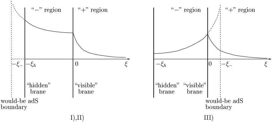
Figure 1: Two-brane setup. Solid line shows the warp factor $(k\mathfrak{s})^{-1}$. Left and right panels correspond to the cases I), II) ($k_{\pm}>0$) and III) ($k_{+}>0\,\ k_{-}<0$), see the text after eq. (18).

As a side remark, it is instructive to consider the reference frame in which the bulk geometry is (locally) static. The coordinates in this frame, $t$ and $r$, are related to $\tau$ and $\xi$ as follows:

$$t = \tau\frac{\mathfrak{c}_{\pm}}{\mathrm{c}_{\pm}}<0\,,$$

$$r = -\tau k_{\pm}\mathfrak{s}_{\pm}\,.$$

Hereafter

$$\mathrm{s}_{\pm}=\sinh\xi_{\pm}\,,\ \ \ \ \mathrm{c}_{\pm}=\cosh\xi_{\pm}\,.$$

Due to one of the Israel junction conditions, one has $k_{-}\mathrm{s_{-}}=k_{+}\mathrm{s}_{+}\equiv H$ (see below), where $H$ is the Hubble parameter on the visible brane given by (16). So, the coordinates $t$, $r$ are continuous across the visible brane. In these coordinates the bulk geometry is described by

$$ds^{2}=\frac{1}{k_{\pm}^{2}r^{2}}(\mathrm{c}_{\pm}^{2}k_{\pm}^{2}dt^{2}-k_{\pm}^{2}d\mathbf{x}^{2}-dr^{2})\,,$$ (5)

which is the Poincaré metric in the two patches of adS_d+2 with different cosmological constants. In this frame the branes are moving. Their positions are given by

$$r_{v}(t)=-Ht\,,\ \ \ \ r_{h}(t)=-Ht\frac{\mathrm{c_{-}}}{\mathrm{s_{-}}}\cdot\frac{\mathrm{s_{h}}}{\mathrm{c}_{h}}\,,$$

where

$$\mathrm{s}_{h}=\sinh(\xi_{-}-\xi_{h})\,,\ \ \ \ \mathrm{c}_{h}=\cosh(\xi_{-}-\xi_{h})\;.$$

Thus, our setup is similar to Refs. [13, 14], where the domain wall moves along $r/t=\mbox{const}$ in the Poincaré coordinates. We do not use the coordinates $r$, $t$ in what follows.

The components of the unperturbed Ricci tensor, calculated with the metric (3), are (hereafter we skip (sub-)superscript “$\pm$” where this does not lead to an ambiguity),

$$R_{\mu\nu}=\frac{(d+1)}{\tau^{2}\mathfrak{s}^{2}}\eta_{\mu\nu}\,,\ \ \ \ R_{\mu\xi}=0\,,\ \ \ \ R_{\xi\xi}=-\frac{d+1}{\mathfrak{s}^{2}}\,,$$

and satisfy the Einstein equations in the bulk

$$R_{AB}=-\frac{\Lambda_{\pm}}{2M^{d}}\cdot\frac{2}{d}\cdot g_{AB},$$ (6)

provided that the values of the inverse adS radii $k_{\pm}$ are related to the cosmological constants,

$$|k_{\pm}|=\sqrt{-\frac{\Lambda_{\pm}}{M^{d}d(d+1)}}.$$ (7)

We take $k_{+}$ positive (without loss of generality) and assume that there is no boundary at $\xi>0$, which implies

$$\xi_{+}>0\;,\;\;\;\;k_{+}>0\;.$$ (8)

Other sign conventions are that in the case $k_{-}>0$ the hidden brane screens the adS boundary at $\xi\to-\xi_{-}$, while for $k_{-}<0$ one can push the hidden brane to infinity. Hence, the two options are

$$\xi_{-}>0\;,\;\;\;\;k_{-}>0\;\;\;\;\mbox{(and}\;\;\xi_{h}<\xi_{-})\;,$$ (9a)

$$\xi_{-}<0\;,\;\;\;\;k_{-}<0\;.$$ (9b)

To proceed, we make use of the Israel junction conditions [34] to determine the boundary conditions on the branes. It is worth recalling the definition of the extrinsic curvature $K_{\mu\nu}$ and the induced metric on the branes (see, e.g., Ref. [35]). Let $F(X^{A})=0$ be the equation of time-like hypersurface $\Sigma$ and $y^{\mu}$ be coordinates on it. We introduce tangent vectors to $\Sigma$

$$e^{A}_{\mu}=\frac{\partial X^{A}}{\partial y^{\mu}}\Bigg{|}_{\Sigma}\,,$$

and the normal unit outer vector

$$n_{A}=-\frac{\partial_{A}F}{\sqrt{|\partial_{B}F\partial^{B}F}|}\,,$$

which is space-like. Then the induced metric and the extrinsic curvature are given by

$$\gamma_{\mu\nu} = e_{\mu}^{A}e_{\nu}^{B}g_{AB}\Big{|}_{\Sigma}\,,$$

$$K_{\mu\nu} = e^{A}_{\mu}e^{B}_{\nu}D_{A}n_{B}\Big{|}_{\Sigma}\,.$$

The Israel junction conditions at each of the branes are

$$\triangle\gamma_{\mu\nu}^{(i)} = 0\,,$$

$$\triangle K_{\mu\nu}^{(i)} = -\frac{\lambda^{(i)}}{2dM^{d}}\gamma_{\mu\nu}^{(i)}\,.$$

Hereafter $\triangle$ denotes a jump of the corresponding quantity across the brane from $\xi>\xi^{(i)}$ to $\xi<\xi^{(i)}$.

Due to $\mathbb{Z}_{2}$ symmetry, the continuity of the induced metric

$$\gamma_{\mu\nu}^{(h)}=\frac{1}{k_{-}^{2}\mathrm{s}_{h}^{2}\tau^{2}}\eta_{\mu\nu}\,,$$

on the hidden brane $(\xi=-\xi_{h})$ is trivially satisfied. The jump of the extrinsic curvature is given by

$$\triangle\gamma^{\nu\rho}_{(h)}K_{\rho\mu}^{(h)}=-2k_{-}\mathrm{c}_{h}\delta^{\nu}_{\mu}=-\frac{\lambda^{(h)}}{2dM^{d}}\delta_{\mu}^{\nu}\,.$$ (10)

Eq. (10) yields a relation between the hidden brane tension and its position:

$$\lambda^{(h)}=4dM^{d}k_{-}\mathrm{c}_{h}\,.$$ (11)

On the visible brane the induced metric and the extrinsic curvature are

$$\gamma_{\mu\nu}^{(v),\pm} = \frac{1}{k^{2}_{\pm}\tau^{2}\mathrm{s_{\pm}}^{2}}\eta_{\mu\nu}\,,$$ (12)

$$\gamma^{\nu\rho}_{(v),\pm}K_{\rho\mu}^{(v),\pm} = -k_{\pm}\mathrm{c_{\pm}}\delta_{\mu}^{\nu}\,.$$ (13)

Then the Israel junction conditions become (using the sign conventions (8) and (9))

$$k_{-}\mathrm{s_{-}}=k_{+}\mathrm{s}_{+}\equiv H\,,$$ (14)

$$k_{+}\mathrm{c_{+}}-k_{-}\mathrm{c_{-}}=\sigma\,,$$ (15)

where

$$\sigma=\frac{\lambda^{(v)}}{2dM^{d}}\;.$$

By solving these equations one gets a relation between the Hubble constant $H$ and the parameters $k_{\pm}$ and $\sigma$,

$$H^{2}=k^{2}\mathrm{s}^{2}=\frac{\left((k_{+}+k_{-})^{2}-\sigma^{2}\right)\left((k_{+}-k_{-})^{2}-\sigma^{2}\right)}{4\sigma^{2}}\,,$$ (16)

and finds

$$\xi_{\pm}=\mathrm{arcsinh}\frac{H}{k_{\pm}}\,.$$ (17)

Three remarks are in order. First, the fact that the solutions (17) exist confirms that the metric (3) with constant $\xi_{\pm}$ is a solution to the Einstein equations and Israel junction conditions. Second, as it follows from (12), the brane is in the de Sitter regime with the Hubble parameter $H\geq 0$ given by (16). Our primary interest in the case $\tau<0$ which corresponds to expanding branes. Most of our formulas, however, are valid also for contracting branes, $\tau>0$. Third, substituting (16), (17) into eq.(15) one gets,

$$\mathrm{sign}(k_{+})|k_{+}^{2}-k_{-}^{2}+\sigma^{2}|-\mathrm{sign}(k_{-})|k_{+}^{2}-k_{-}^{2}-\sigma^{2}|=2|\sigma|\sigma\,.$$ (18)

For $k_{+}>0$ this equation together with the condition $H\geq 0$ leads, in general, to the following three cases:

• $k_{+}>0$, $k_{-}>0$, $\sigma>0$   $\Longrightarrow$    $k_{+}\geq k_{-}+\sigma$,     $\xi_{+},\xi_{-}>0$;

• $k_{+}>0$, $k_{-}>0$, $\sigma<0$   $\Longrightarrow$   $0<k_{+}\leq k_{-}-|\sigma|$,     $\xi_{+},\xi_{-}>0$

• $k_{+}>0$, $k_{-}<0$, $\sigma>0$   $\Longrightarrow$   $0<k_{+}\leq\sigma-|k_{-}|$,     $\xi_{+}>0$, $\xi_{-}<0$  ,

which is consistent with our sign convention (8), (9).

To conclude this section let us consider the static limit $H\to 0$. To this end we require that the resulting background metric takes the form (5) with $\mathrm{c}_{\pm}\to 1$, and that the visible brane is located at $r_{v}=1$ while the hidden one is at $r_{h}$. In all three cases I)-III) discussed above the limit $H\to 0$ is approached in the following regime (see (15), (17)):

$$\xi_{\pm}\simeq\frac{H}{k_{\pm}}\to 0\,,\ \ \ k_{+}-k_{-}\to\sigma\,,\ \ \ H|\tau|\to 1\,,\ \ \ \xi_{-}-\xi_{h}\to\xi_{-}r_{h}\,.$$ (19)

In the limit (19) the relations between the brane tensions and their positions, eqs. (11) and (16), (17), reduce to the well-known fine tuning conditions between the brane tensions and the bulk cosmological constants, $\lambda^{(h)}=4dM^{d}k_{-}$, $\lambda^{(v)}=2dM^{d}(k_{+}-k_{-})$.

3 Perturbations and gauge

Let us consider small perturbations of the metric (3)

$$g_{AB}\to\left\{\begin{array}[]{l}g_{\mu\nu}+\displaystyle\frac{\hat{h}_{\mu\nu}}{k_{\pm}^{2}\mathfrak{s}^{2}_{\pm}\tau^{2}}\\ \\ g_{\xi A}+\hat{h}_{\xi A}\,,\end{array}\right.$$

and begin with the coordinate frame $(\hat{x}^{\mu},\hat{\xi})$ in which the visible brane is placed at $\hat{\xi}=b(\hat{x})$ while the hidden brane is still at $\hat{\xi}=-\xi_{h}$. We do not assume that $\hat{h}_{AB}$ is continuous across the brane but the induced metric

$$\hat{\gamma}_{\mu\nu}=\frac{1}{k_{\pm}^{2}\hat{\tau}^{2}\mathrm{s}^{2}_{\pm}}\left(\eta_{\mu\nu}\left(1-2\frac{\mathrm{c}_{\pm}}{\mathrm{s}_{\pm}}b\right)+\hat{h}_{\mu\nu}\right)\,,$$

should be continuous (the first Israel junction condition). Note that due to the condition (14), the coordinates $(\hat{x}^{\mu},\hat{\xi})$ continuously cover the whole space.

As an intermediate step, let us demonstrate that there is a gauge in which the new coordinates $(\tilde{x}^{\mu},\tilde{\xi})$ cover the whole space, the visible brane is straight and placed at $\tilde{\xi}=0$, the hidden brane is at $\tilde{\xi}=-\xi_{h}$, and $\tilde{h}_{AB}$ is continuous. The linear gauge transformation $\delta h_{AB}(\tilde{X})=\tilde{h}_{AB}(\tilde{X})-\hat{h}_{AB}(\tilde{X})$ of the metric perturbation under coordinate transformation $\tilde{X}^{A}=\hat{X}^{A}+\zeta^{A}$ is

$$\delta h_{\xi\xi} = -\frac{2}{\mathfrak{s}}(\mathfrak{s}\zeta_{\xi})^{\prime}\,,$$ (20a)

$$\delta h_{\xi\mu} = -\partial_{\mu}\zeta_{\xi}-\frac{1}{\mathfrak{s}^{2}k^{2}\tau^{2}}\zeta_{\mu}^{\prime}\,,$$ (20b)

$$\delta h_{\mu\nu} = -\partial_{(\mu}\zeta_{\nu)}+\frac{2}{\tau}\zeta_{0}\eta_{\mu\nu}-2k^{2}\mathfrak{c}\mathfrak{s}\zeta_{\xi}\eta_{\mu\nu}\,.$$

Hereafter $(d+1)$-dimensional indices are lowered and raised by $\eta_{\mu\nu}$, $\xi$-index is lowered and raised by $g_{AB}$, e.g., $\zeta_{\xi}=g_{\xi\xi}\zeta^{\xi}=-\zeta^{\xi}/k^{2}\mathfrak{s}^{2}$, prime denotes the derivative with respect to $\xi$, and $a_{(\mu}b_{\nu)}=a_{\mu}b_{\nu}+a_{\nu}b_{\mu}$.

Let us make the following continuous coordinate transformations:

$$\tilde{\xi} = \hat{\xi}-b\cdot\chi(\tilde{\xi})\,,$$

$$\tilde{x}^{\mu} = \hat{x}^{\mu}+\zeta^{\mu}\,,$$

where $\chi(\tilde{\xi})$ is yet an arbitrary continuous function satisfying the conditions

$$\chi(-\xi_{h})=0\,,\ \ \ \ \chi(0)=1.$$

Then the visible brane is placed at

$$\tilde{\xi}=0\,,$$

while the coordinate of the hidden brane is left intact $\tilde{\xi}=-\xi_{h}$.

In this coordinate frame the jumps of $\tilde{h}_{A\xi}$ across the visible brane are

$$\triangle\tilde{h}_{\xi\xi}(\tilde{x},\tilde{\xi}) = \triangle\hat{h}_{\xi\xi}(\tilde{x},\tilde{\xi})-2b\triangle\frac{1}{k^{2}\mathfrak{s}}\left(\frac{\chi}{\mathfrak{s}}\right)^{\prime}\bigg{|}_{\tilde{\xi}=0}\,,$$

$$\triangle\tilde{h}_{\mu\xi}(\tilde{x},\tilde{\xi}) = \triangle\hat{h}_{\mu\xi}(\tilde{x},\tilde{\xi})-\frac{1}{k^{2}\mathrm{s}^{2}\tau^{2}}\triangle\zeta_{\mu}^{\prime}\bigg{|}_{\tilde{\xi}=0}\,.$$

We see that the zero jump equations $\triangle\tilde{h}_{A\xi}=0$ can be satisfied by an appropriate choice of derivatives $\zeta_{\mu}^{\prime}$ and $\chi^{\prime}$ on the brane. Then one has $\triangle\tilde{h}_{\mu\nu}=0$ automatically, due to the first junction condition.

$h_{A\xi}=0$ gauge.

As a final step, we make the second continuous gauge transformation which gets rid of $h_{A\xi}$ in the whole space. We write

$$\xi=\tilde{\xi}+\zeta^{\xi}\,,\ \ \ \ x^{\mu}=\tilde{x}^{\mu}+\zeta^{\mu}\,,$$ (21)

and require $h_{A\xi}=0$. Then, by making use of eq. (20a), one finds from the condition $h_{\xi\xi}=0$ that

$$\zeta_{\xi}=\frac{1}{2\mathfrak{s}}\int\limits_{0}^{\xi}\mathfrak{s}\tilde{h}_{\xi\xi}d\xi+\frac{\varepsilon_{\xi}(x)}{\mathfrak{s}}\equiv\zeta_{\xi}^{(I)}+\frac{\varepsilon_{\xi}(x)}{\mathfrak{s}}\,,$$

where $\varepsilon_{\xi}(x)$ is in general different in the different regions. In the “$-$” region, $\varepsilon_{\xi}^{-}$ cannot vanish and is determined by the requirement that the hidden brane is left intact: $\zeta^{\xi}(-\xi_{h})=0$, that is

$$\varepsilon^{-}_{\xi}(x)=\frac{1}{2}\int\limits_{-\xi_{h}}^{0}\mathfrak{s}\tilde{h}_{\xi\xi}d\xi.$$ (22)

The function $\varepsilon_{\xi}^{+}(x)$ is determined by the continuity of $\zeta^{\xi}$ across the visible brane,

$$k_{-}\varepsilon_{\xi}^{-}=k_{+}\varepsilon_{\xi}^{+}\,.$$ (23)

The condition $h_{\mu\xi}=0$ and eq. (20b) give

$$\zeta_{\mu}=k^{2}\tau^{2}\int\limits_{0}^{\xi}(\tilde{h}_{\mu\xi}-\partial_{\mu}\zeta^{(I)}_{\xi})\mathfrak{s}^{2}d\xi+k^{2}\tau^{2}\partial_{\mu}\varepsilon_{\xi}\cdot(\mathrm{c}-\mathfrak{c})+\varepsilon_{\mu}(x)\,.$$

The continuity of $\zeta^{\mu}$ requires that $\varepsilon_{\mu}(x)$ is continuous.

Two remarks are in order. First, we note that $\varepsilon_{\mu}(x)$ can be regarded as a residual gauge transformation,

$$h_{\mu\nu}\to h_{\mu\nu}-\partial_{(\mu}\varepsilon_{\nu)}+\frac{2}{\tau}\varepsilon_{0}\eta_{\mu\nu}\,,$$ (24)

which does not touch the branes and is consistent with the gauge $h_{A\xi}=0$.

Second, arbitrary functions $\varepsilon_{\xi}^{\pm}(x)$ (which do not necessarily satisfy the conditions (22), (23)) can be considered as a gauge transformation,

$$h_{\mu\nu}\to h_{\mu\nu}-(\mathrm{c}-\mathfrak{c})\cdot(2k^{2}\tau^{2}\partial_{\mu}\partial_{\nu}\varepsilon_{\xi}+2k^{2}\tau\delta_{(\mu 0}\partial_{\nu)}\varepsilon_{\xi}-2k^{2}\tau\eta_{\mu\nu}\partial_{\tau}\varepsilon_{\xi})-2k^{2}\mathfrak{c}\eta_{\mu\nu}\varepsilon_{\xi}\,,$$ (25)

which is consistent with the gauge $h_{A\xi}=0$. So, the Einstein equations in the bulk, being written in the gauge $h_{A\xi}=0$, are invariant under this transformation. However, these gauge transformations in general shift the branes. In particular, with the transformations (22), (23) the hidden brane is left intact while the new position of the visible brane is determined at $\xi^{(v)}=\zeta^{\xi}(x,0)$ or

$$\xi^{(v)}=f(x)\,,$$ (26)

where

$$f(x)=-k^{2}\mathrm{s}\varepsilon_{\xi}$$

is nothing but the radion. It follows from its definition that the radion should be continuous across the brane (and it is indeed continuous due to (14) and (23)).

In what follows we use continuous coordinates $(x^{\mu},\xi)$ (see (21)), work in the gauge $h_{A\xi}=0$, and place the hidden brane at $\xi=-\xi_{h}$, while the position of the visible brane is given by (26). Our purpose is to derive equation of motion for the radion and study its properties. To this end we need to find solutions to the perturbed bulk Einstein equations and Israel junction conditions.

4 Einstein equations

Taking into account (7) we write the bulk Einstein equations (6) in the form

$$\mathcal{E}_{AB}\equiv R_{AB}-k^{2}(d+1)g_{AB}=0\,.$$ (27)

In what follows we use the standard helicity decomposition of the metric perturbation,

$$h_{00} = 2\Phi\,,$$

$$h_{0i} = \partial_{i}Z+Z_{i}\,,$$

$$h_{ij} = -2\Psi\delta_{ij}+2\partial_{i}\partial_{j}E+\partial_{(i}W_{j)}+h_{ij}^{TT}\,,$$

where $Z_{i}$, $W_{i}$ are transverse and $h_{ij}^{TT}$ is transverse and traceless

$$\partial_{i}Z_{i}=\partial_{i}W_{i}=\partial_{i}h_{ij}^{TT}=h_{ii}^{TT}=0\,.$$

In terms of these functions the linearized Einstain equations (27) are

$$\delta\mathcal{E}_{00} = \partial^{2}\Phi-\frac{d\dot{\Phi}}{\tau}+\frac{2d\Phi}{\tau^{2}}-d\ddot{\Psi}+\frac{d\dot{\Psi}}{\tau}+\partial^{2}\ddot{E}-\frac{\partial^{2}\dot{E}}{\tau}-\partial^{2}\dot{Z}+\frac{\partial^{2}Z}{\tau}$$ (28a)

$$+\frac{\hat{O}_{\xi}\Phi}{\tau^{2}}-\frac{\mathfrak{c}}{2\tau^{2}\mathfrak{s}}h^{\prime}\,,$$

$$\delta\mathcal{E}_{0i} = \partial_{i}\left(-\frac{d-1}{\tau}\Phi-(d-1)\dot{\Psi}+\frac{1}{2\tau^{2}}\hat{O}_{\xi}Z\right)+\frac{1}{2}\partial^{2}(Z_{i}-\dot{W}_{i})+\frac{1}{2\tau^{2}}\hat{O}_{\xi}Z_{i}\,,$$ (28b)

$$\delta\mathcal{E}_{ij} = \delta_{ij}\left(\Box\Psi-\frac{(2d-1)}{\tau}\dot{\Psi}+\frac{1}{\tau^{2}}\partial^{2}(\dot{E}-Z)+\frac{\dot{\Phi}}{\tau}-\frac{2d\Phi}{\tau^{2}}-\frac{\hat{O}_{\xi}\Psi}{\tau^{2}}+\frac{\mathfrak{c}}{2\tau^{2}\mathfrak{s}}h^{\prime}\right)$$ (28e)

$$+\partial_{i}\partial_{j}\left(\dot{Z}-\frac{(d-1)Z}{\tau}-(d-2)\Psi-\Phi-\ddot{E}+\frac{(d-1)\dot{E}}{\tau}+\frac{\hat{O}_{\xi}E}{\tau^{2}}\right)$$

$$+\frac{1}{2}\left(\partial_{(i}\dot{Z}_{j)}-\frac{(d-1)\partial_{(i}Z_{j)}}{\tau}-\partial_{(i}\ddot{W}_{j)}+\frac{(d-1)\partial_{(i}\dot{W}_{j)}}{\tau}+\frac{\hat{O}_{\xi}\partial_{(i}W_{j)}}{\tau^{2}}\right)$$

$$-\frac{1}{2}\left(\Box h_{ij}^{TT}-\frac{(d-1)\dot{h}_{ij}^{TT}}{\tau}-\frac{\hat{O}_{\xi}h_{ij}^{TT}}{\tau^{2}}\right)\,,$$

$$\delta\mathcal{E}_{0\xi} = \left(\partial^{2}\dot{E}-\frac{\partial^{2}E}{\tau}-\frac{\partial^{2}Z}{2}-\frac{d\Phi}{\tau}-d\dot{\Psi}+\frac{d\Psi}{\tau}\right)^{\prime}\,,$$ (28f)

$$\delta\mathcal{E}_{i\xi} = \partial_{i}\left(\frac{\dot{Z}}{2}-\frac{(d+1)Z}{2\tau}-\Phi-(d-1)\Psi\right)^{\prime}+\frac{1}{2}\left(\dot{Z}_{i}-\frac{(d+1)Z_{i}}{\tau}-\partial^{2}W_{i}\right)^{\prime}\,,$$ (28g)

$$\delta\mathcal{E}_{\xi\xi} = -\mathfrak{s}\left(\frac{h^{\prime}}{2\mathfrak{s}}\right)^{\prime}\,.$$ (28h)

Hereafter we use the following notations,

$$h=h_{\mu}^{\mu}=2\Phi+2d\Psi-2\partial^{2}E\,,\ \ \ \partial^{2}=\partial_{i}\partial_{i}\,,\ \ \ \Box=\partial^{\mu}\partial_{\mu}=\partial_{0}^{2}-\partial^{2}\,,$$

$$\hat{O}_{\xi}=\partial_{\xi}^{2}-d\frac{\mathfrak{c}}{\mathfrak{s}}\partial_{\xi}=\mathfrak{s}^{d}\partial_{\xi}\frac{1}{\mathfrak{s}^{d}}\partial_{\xi}\,,$$

and dot denotes derivative with respect to $\tau$.

Scalars.

The scalar part of eqs. (28) can be significantly simplified by using variables which are invariant under the residual gauge transformations (24). Let us set $\varepsilon_{i}=\partial_{i}\varepsilon$, then the scalar functions transform as follows,

$$\delta_{\varepsilon}\Phi=-\tau\partial_{\tau}\left(\frac{\varepsilon_{0}}{\tau}\right)\,,\ \ \ \delta_{\varepsilon}\Psi=\frac{\varepsilon_{0}}{\tau}\,,\ \ \ \delta_{\varepsilon}E=-\varepsilon\,,\ \ \ \delta_{\varepsilon}Z=-\varepsilon_{0}-\dot{\varepsilon}\,.$$

There are two independent gauge-invariant variables. It is convenient to use the following pair:

$$A=\frac{Z-\dot{E}}{\tau}+\Psi\,,\ \ \ \ B=\dot{Z}-\ddot{E}+\Psi-\Phi\,.$$

Let us introduce the combination,

$$\frac{U}{2\tau^{2}}=d\hat{O}_{\tau}A+\partial^{2}B-\frac{d\dot{B}}{\tau}+\frac{d(d+1)B}{\tau^{2}}\,,$$

where

$$\hat{O}_{\tau}=\Box-\frac{(d-1)\partial_{\tau}}{\tau}-\frac{(d+1)}{\tau^{2}}\,.$$

In terms of these variables, the linearized Einstein equations in the scalar sector take the form

$$\delta\mathcal{E}_{00}: \partial^{2}A-d\ddot{A}+\frac{2dA}{\tau^{2}}+\frac{d\dot{B}}{\tau}-\frac{2dB}{\tau^{2}}=-\frac{\hat{O}_{\xi}\Phi}{\tau^{2}}+\frac{\mathfrak{c}}{2\tau^{2}\mathfrak{s}}h^{\prime}\,,$$ (29a)

$$\delta\mathcal{E}_{0i}: -\frac{(d-1)}{\tau}(\tau\dot{A}+A-B)=-\frac{\hat{O}_{\xi}Z}{2\tau^{2}}\,,$$ (29b)

$$\delta\mathcal{E}_{ij}(\delta_{ij}): \Box A-\frac{2(d-1)\dot{A}}{\tau}-\frac{2dA}{\tau^{2}}-\frac{\dot{B}}{\tau}+\frac{2dB}{\tau^{2}}=\frac{\hat{O}_{\xi}\Psi}{\tau^{2}}-\frac{\mathfrak{c}}{2\tau^{2}\mathfrak{s}}h^{\prime}\,,$$ (29c)

$$\delta\mathcal{E}_{ij}(\partial_{i}\partial_{j}): -(d-1)A+B=-\frac{\hat{O}_{\xi}E}{\tau^{2}}\,,$$ (29d)

$$\tau^{d-1}\partial_{\mu}\frac{\delta\mathcal{E}_{\xi}^{\mu}}{\tau^{d-1}}: \frac{1}{2\tau^{2}}(U+dh)^{\prime}=0\,,$$ (29e)

$$\delta\mathcal{E}_{\mu}^{\mu}: \frac{U}{\tau^{2}}=\frac{\hat{O}_{\xi}h}{2\tau^{2}}-\frac{\mathfrak{c}(d+1)}{2\tau^{2}\mathfrak{s}}h^{\prime}\,.$$ (29f)

Eqs. (28h), (29e), (29f) yield

$$U=-d\frac{\mathfrak{c}}{\mathfrak{s}}h^{\prime}\,.$$ (30)

Combining eqs. (29a) – (29d) and their time derivatives and taking into account (30) we finaly obtain the following set of equations for $A$ and $B$:

$$\hat{O}_{\tau}B+\frac{4\dot{B}}{\tau}+\frac{4B}{\tau^{2}} = \frac{1}{\tau^{2}}(\hat{O}_{\xi}+d-1)B\,,$$ (31a)

$$\frac{\dot{B}}{\tau}-\frac{(d-3)B}{\tau^{2}}-\frac{\partial^{2}B}{d} = \frac{1}{\tau^{2}}(\hat{O}_{\xi}+d-1)A\,.$$ (31b)

5 Linearized Israel junction conditions

5.1 Boundary conditions at $\xi=-\xi_{h}$

Due to $\mathbb{Z}_{2}$ symmetry, the continuity of the induced metric at the hidden brane

$$\gamma_{\mu\nu}^{(h)}=\frac{1}{k_{-}^{2}\mathrm{s}_{h}^{2}\tau^{2}}(\eta_{\mu\nu}+h_{\mu\nu}(-\xi_{h}))\,,$$

is trivially satisfied. The jump of the perturbed extrinsic curvature is given by

$$-\triangle\delta[\gamma^{\nu\rho}_{(h)}K_{\rho\mu}^{(h)}]=-k_{-}\mathrm{s}_{h}h^{\nu^{\prime}}_{\mu}=0\,.$$

Thus, one has

$$h_{\mu\nu}^{\prime}\big{|}_{\xi=-\xi_{h}}=0\,.$$ (32)

This means, in particular, that $h^{\prime}\big{|}_{\xi=-\xi_{h}}=0$. Together with eq. (28h) this yields

$$h^{\prime}=0\ \ \mbox{at}\ \ -\xi_{h}\leq\xi\leq 0\,.$$ (33)

5.2 Junction equations at the visible brane

The Israel junction conditions at the visible brane have the form

$$\triangle\gamma_{\mu\nu}^{(v)} = 0\,,$$ (34a)

$$\triangle K_{\mu\nu}^{(v)} = -\sigma\gamma_{\mu\nu}^{(v)}\,.$$ (34b)

The perturbed induced metric on the brane (at $\xi=f(x)$) is given by

$$\gamma_{\mu\nu}^{(v),\pm}=\frac{1}{k_{\pm}^{2}\tau^{2}\mathrm{s_{\pm}}^{2}}\left(\eta_{\mu\nu}\left(1-2\frac{\mathrm{c}_{\pm}}{\mathrm{s}_{\pm}}f\right)+h_{\mu\nu}^{\pm}\right)\,,$$

and the extrinsic curvature is

$$\gamma^{\nu\rho}_{(v)}K_{\rho\mu}^{(v)}=-k\mathrm{c}\delta_{\mu}^{\nu}+k\mathrm{s}\left(\tau^{2}\partial_{\mu}\partial^{\nu}f-\tau(\delta_{\mu}^{\nu}\dot{f}-\delta_{(\mu 0}\partial^{\nu)}f)-\delta_{\mu}^{\nu}f+\frac{h_{\mu}^{\nu^{\prime}}}{2}\right)\,.$$

The junction conditions (34), are satisfied for the unperturbed background. Hence, for the linearized part we have

$$\triangle\delta\gamma_{\mu\nu}^{(v)} = 0\,,$$

$$\triangle\delta[\gamma^{\nu\rho}_{(v)}K_{\rho\mu}^{(v)}] = 0\,.$$ (35)

Calculating the trace $K=\gamma^{\mu\rho}_{(v)}K_{\mu\rho}^{(v)}$ we get

$$K=-k\mathrm{c}(d+1)+k\mathrm{s}\tau^{2}\left(\hat{O}_{\tau}f+\frac{h^{\prime}}{2\tau^{2}}\right)\,.$$ (36)

By making use the Gauss-Codazzi relation

$$2G_{AB}n^{A}n^{B}=k_{\pm}^{2}d(d+1)=^{(d+1)}R-(K_{\mu\nu}^{\pm(v)}K_{\pm(v)}^{\mu\nu}-K_{\pm}^{2})\,,$$ (37)

where $G_{AB}$ is the Einstein tensor, ${}^{(d+1)}R$ is the curvature scalar on the brane, and $K^{\mu\nu}_{(v)}\equiv\gamma^{\mu\rho}_{(v)}\gamma^{\nu\lambda}_{(v)}K_{\rho\lambda}^{(v)}$, one finds

$$\triangle\delta(K_{\mu\nu}^{(v)}K^{\mu\nu}_{(v)}-K^{2})=0\,.$$ (38)

Due to the fact that the background extrinsic curvature is proportional to $\eta_{\mu\nu}$ (cf. (13)), it is straightforward to check that eq. (38) takes the form

$$-\triangle\left[2dk\mathrm{c}\cdot\delta K\right]=0\,.$$

Together with eq. (35) this leads to the equation

$$\delta K_{\pm}=0\,,$$

and, therefore,

$$\hat{O}_{\tau}f=0\,,$$ (39)

where we have used (33). This is the desired radion equation of motion.

Besides that, the junction conditions yield

$$\triangle h_{\mu\nu} = 2\triangle\frac{\mathrm{c}}{\mathrm{s}}\eta_{\mu\nu}f=2\frac{\sigma}{H}\eta_{\mu\nu}f\,,$$ (40)

$$\triangle h_{\mu\nu}^{\prime} = 0\,.$$

From the latter equation and eqs. (28h), (29f), (33) we find

$$h^{\prime}=0\,,\ \ \ \ U=0$$ (41)

in the whole space.

The condition (40) translates into

$$\triangle\Phi=\triangle\Psi=\triangle A=\frac{\sigma}{H}f\,,$$ (42)

while other functions characterizing the metric perturbations, as well as all first derivatives of $h_{\mu\nu}$ with respect to $\xi$ are continuous across the brane.

6 Solutions

6.1 Scalar sector

Now we are ready to solve the linearized Einstein equations. We begin with eq. (31a). The variables separate, so the modes have the form

$$B_{\kappa}(x,\xi)=b_{\kappa}(x)\beta_{\kappa}(\xi)\,,$$

where $\beta_{\kappa}$ are normalizable (since $B$ is gauge invariant),

$$\int\limits_{-\xi_{h}}^{\infty}\frac{d\xi}{(k\mathfrak{s})^{d}}|\beta_{\kappa}|^{2}<\infty\,,$$

and continuous together with their derivatives across the brane (see eq. (42)):

$$\triangle\beta_{\kappa}(0)=\triangle\beta_{\kappa}^{\prime}(0)=0\,.$$

They are solutions to the eigenvalue equation

$$(\hat{O}_{\xi}+d-1)\beta_{\kappa}=-\nu\beta_{\kappa}\,.$$ (43)

Explicitly,

$$\mathfrak{s}^{d}\frac{\partial}{\partial\xi}\frac{1}{\mathfrak{s}^{d}}\frac{\partial}{\partial\xi}\beta_{\kappa}+\left(\frac{d^{2}}{4}-\kappa^{2}\right)\beta_{\kappa}=0$$ (44)

with

$$\kappa=\frac{\sqrt{(d-2)^{2}-4\nu}}{2}\;.$$

We show in Appendix A that there is one constant discrete mode in the spectrum with $\kappa=d/2$ ($\nu=1-d$),

$$\beta_{\frac{d}{2}}(\xi)=\mathrm{const}\,.$$ (45)

For $k_{-}>0$ it is localized near the hidden brane. However, as we discuss later on, this mode does not generate a solution to the complete set of the Einstein equations (29), so the corresponding metric perturbations are, in fact, absent. The rest of the spectrum is continuous and starts from zero: $\kappa^{2}\leq 0$ ($\nu\geq(d-2)^{2}/4$). The $x^{\mu}$-dependent parts

$$b_{\kappa}(x)=b_{\kappa}(\tau,\mathbf{p})\mathrm{e}^{i\mathbf{px}}\,,$$

satisfy the following equation,

$$\left(\partial_{\tau}^{2}+p^{2}-\frac{(d-5)\partial_{\tau}}{\tau}-\frac{(d-3-\nu)}{\tau^{2}}\right)b_{\kappa}(\tau,\mathbf{p})=0\,.$$ (46)

Let us now consider eq. (31b). For non-vanishing left hand side this equation immediately yields

$$A_{\kappa}(\tau,\mathbf{p},\xi)=a_{\kappa}(\tau,\mathbf{p})\beta_{\kappa}(\xi)\,,$$ (47)

with

$$a_{\kappa}(\tau,\mathbf{p})=\frac{1}{d\nu}\left(d(d-3)-d\tau\partial_{\tau}-p^{2}\right)b_{\kappa}(\tau,\mathbf{p})\,.$$ (48)

There is an imporant subtlety here. The modes (47) are continuous across the visible brane and hence contribute to the continuous part of the function $A$ only. This continuous part of $A$ satisfies eq. (42) with vanishing right hand side. To satisfy eq. (42) with non vanishing right hand side, we note that the operator $\hat{O}_{\xi}+d-1$ has yet another zero mode (in addition to (45)) when it acts in the space of discontinuous functions. In that case both sides of eq. (31b) are equal to zero, and hence the relations (47), (48) are no longer valid.

Thus, we search for the solution of the form

$$A_{\frac{d-2}{2}}(x,\xi)=f(x)\beta_{\frac{d-2}{2}}(\xi)\,,\ \ \ \ B_{\frac{d-2}{2}}(x,\xi)=0\,,$$ (49)

where the second equality follows from the fact that eqs. (31) do not admit non-trivial solution for $B$ in the case of vanishing right hand side of eq. (31b). The function $\beta_{\frac{d-2}{2}}(\xi)$ must obey eq. (43) in both “+” and “-” regions and has the jump at the visible brane

$$\triangle\beta_{\frac{d-2}{2}}=\frac{\sigma}{H}\;.$$ (50)

The boundary condition at the hidden brane follows from (32):

$$\beta^{\prime}_{\frac{d-2}{2}}(-\xi_{h})=0\;.$$ (51)

To construct the new zero mode we note that two linear independent solutions to eq. (44) with $\kappa=(d-2)/2$ ($\nu=0$) are

$$\beta_{\frac{d-2}{2}}^{(1)} = \mathfrak{c}^{d-1}\left(\frac{\mathfrak{s}}{\mathfrak{c}}\right)^{d+1}F\left(1,\frac{3}{2};\frac{d+3}{2};\frac{\mathfrak{s}^{2}}{\mathfrak{c}^{2}}\right)\,,$$ (52a)

$$\beta_{\frac{d-2}{2}}^{>} = \mathfrak{c}\;,$$ (52b)

where $F$ is the hypergeometric function. At large $\xi$, $\beta_{\frac{d-2}{2}}^{(1)}$ grows as $\mathrm{e}^{(d-1)\xi}$ and hence it cannot be used in the “+” region. In contrast, the second solution $\beta_{\frac{d-2}{2}}^{>}$ is sutable at large $\xi$. In the “$-$” region the following linear combination of (52) satisfies (51):

$$\beta_{\frac{d-2}{2}}^{<}(\xi)=\beta_{\frac{d-2}{2}}^{(1)}(\xi)-\mathfrak{c}_{-}\frac{\beta_{\frac{d-2}{2}}^{(1)^{\prime}}(-\xi_{h})}{\mathrm{s}_{h}}\;.$$ (53)

By making use of the boundary condition (50) at $\xi=0$ we finaly obtain

$$\beta_{\frac{d-2}{2}}(\xi)=\left\{\begin{array}[]{l}\displaystyle{\frac{\sigma}{H}\left(\mathrm{s}_{+}\left[\frac{\mathrm{c_{+}}}{\mathrm{s_{+}}}-\frac{\beta_{\frac{d-2}{2}}^{<}(0)}{\beta_{\frac{d-2}{2}}^{<^{\prime}}(0)}\right]\right)^{-1}\mathfrak{c}_{+}}\ \ ~{}~{}\mbox{at}\ \ \xi>0\,,\\ \\ \displaystyle{\frac{\sigma}{H}\left(\beta_{\frac{d-2}{2}}^{<^{\prime}}(0)\left[\frac{\mathrm{c_{+}}}{\mathrm{s_{+}}}-\frac{\beta_{\frac{d-2}{2}}^{<}(0)}{\beta_{\frac{d-2}{2}}^{<^{\prime}}(0)}\right]\right)^{-1}\beta_{\frac{d-2}{2}}^{<}(\xi)}\ \ ~{}~{}\mbox{at}\ \ \xi<0\,,\end{array}\right.$$ (54)

In both of these formulas, $\beta_{\frac{d-2}{2}}^{<}(0)$ and $\beta_{\frac{d-2}{2}}^{<^{\prime}}(0)$ are the limiting values in the “-” region. To end up with the analysis of the zero mode, we note that the Wronskian $\mathcal{W}(f_{1},f_{2})=f_{1}f_{2}^{\prime}-f_{1}^{\prime}f_{2}$ of the functions (52) is

$$\mathcal{W}(\mathfrak{c},\beta_{\frac{d-2}{2}}^{(1)})=\mathcal{W}(\mathfrak{c},\beta_{\frac{d-2}{2}}^{<})=(d+1)\mathfrak{s}^{d}\,.$$ (55)

Note also that the terms proportional to $\mathfrak{c}_{\pm}$ in (54) correspond to the gauge transformation that preserves $h_{\xi\xi}=0$ (cf. eq. (25)). In particular, the radion is pure gauge in the “+” region outside the visible brane, i.e., the non-trivial part of its wave function is concentrated on and between the branes.

Let us now come back to the constant mode (45) and consider eqs. (29b), (29d). These equations can be viewed as inhomogeneous equations for $Z$ and $E$, respectively. Recall that the operator $\hat{O}_{\xi}$ has exactly one zero mode $\beta_{d/2}$. The necessary condition for the existence of solutions to eqs. (29b), (29d) is the orthogonality of the inhomogeneity to this mode, and it cannot be satisfied if $A$ and/or $B$ contain contributions proportional to $\beta_{d/2}$. Thus, we are forced to conclude that $B$ contains the continuous part of the spectrum of (43) only. On the contrary, the (discontinuous) zero mode $\beta_{\frac{d-2}{2}}$, contributing to $A$, is orthogonal to $\beta_{d/2}$. Indeed, by making use of (43), (45), integrating by parts and taking into account the boundary conditions at $-\xi_{h}$ and at infinity, we write

$$\langle\beta_{\frac{d}{2}}|\beta_{\frac{d-2}{2}}\rangle=\beta_{\frac{d}{2}}\cdot\int\limits_{-\xi_{h}}^{\infty}\frac{d\xi}{(k\mathfrak{s})^{d}}\frac{\hat{O}_{\xi}\beta_{\frac{d-2}{2}}}{1-d}=\beta_{\frac{d}{2}}\cdot\frac{\triangle\beta_{\frac{d-2}{2}}^{\prime}(0)}{k\mathrm{s}(d-1)}=0\,.$$

The last point to check is that $U$ and $h^{\prime}$ vanish, eq. (41). Using eqs. (46), (48) one directly finds that eq. (41) indeed holds for the modes with $\nu\neq 0$. For the zero mode (49), eq. (41) is satisfied due to the radion equation of motion (39).

Explicit expressions for the metric components induced by the radion can be found by making use eqs. (29a) – (29d). Let $Q(\xi)$ be a continuous solution to the equation

$$\hat{O}_{\xi}Q=\beta_{\frac{d-2}{2}}(\xi)$$

with boundary conditions

$$Q^{\prime}(-\xi_{h})=0\,,\ \ \ \frac{Q(\xi)}{\mathfrak{s}_{+}^{d/2}}\bigg{|}_{\xi\to\infty}\to 0\,.$$

Explicitly,

$$Q(\xi)=\frac{\beta_{\frac{d-2}{2}}(\xi)}{1-d}+\Theta(-\xi)\frac{\sigma}{H(1-d)}+\mbox{const}\,,$$

where $\Theta$ is the step function; the last constant term cannot be fixed and corresponds to the residual gauge transformation (24). Then

$$\Phi = f\beta_{\frac{d-2}{2}}+(d-1)(\tau^{2}\ddot{f}+\tau\dot{f})\cdot Q\,,$$

$$\Psi = f\beta_{\frac{d-2}{2}}-(d-1)\tau\dot{f}\cdot Q\,,$$

$$E = (d-1)\tau^{2}f\cdot Q\,,$$

$$Z = 2(d-1)(\tau^{2}\dot{f}+\tau f)\cdot Q\,.$$

6.2 Vector sector

Let us introduce the following gauge invariant variable:

$$V_{i}=Z_{i}-\dot{W}_{i}\,.$$

Then the Einstein equations in the vector sector are

$$\Box V_{i}-\frac{(d-3)\dot{V}_{i}}{\tau}=\frac{1}{\tau^{2}}(\hat{O}_{\xi}+d-1)V_{i}\,,$$ (56a)

$$\partial^{2}V_{i}=-\frac{\hat{O}_{\xi}Z_{i}}{\tau^{2}}\,,$$ (56b)

$$\left(\dot{Z}_{i}-\frac{(d+1)Z_{i}}{\tau}-\partial^{2}W_{i}\right)^{\prime}=0\,.$$ (56c)

The situation is reminiscent of that in the scalar sector. Any solution to eq. (56a) can be decomposed in eigenfunctions $\beta_{\kappa}(\xi)$. However, the contribution from the localized mode $\beta_{d/2}$ vanishes due to the second equation (56b): $V_{i}$ should be orthogonal to $\beta_{d/2}$. Then the validity of the third equation (56c) can be directly verified. Thus, all vector modes belong to the continuous part of the spectrum of the operator (43), and hence they are delocalized.

6.3 Tensor sector

The only equation in the tensor sector is

$$\Box h_{ij}^{TT}-\frac{(d-1)\dot{h}_{ij}^{TT}}{\tau}+\frac{(d-1)h_{ij}^{TT}}{\tau^{2}}=\frac{1}{\tau^{2}}(\hat{O}_{\xi}+d-1)h_{ij}^{TT}\,.$$

Therefore, there are no conditions eliminating the discrete mode $\beta_{d/2}$ which in the case $k_{-}>0$ is localized near the hidden brane. By writing

$$h_{(\kappa)ij}^{TT}(X)=\beta_{\kappa}(\xi)\cdot e_{ij}\cdot\mathcal{H}_{\kappa}(\tau,\mathbf{p})\mathrm{e}^{i\mathbf{px}}\,,$$

where $e_{ij}$ is constant transverse-traceless polarization tensor, one finds the equation for $\mathcal{H}_{d/2}$:

$$\left(\partial^{2}_{\tau}+p^{2}-\frac{(d-1)\partial_{\tau}}{\tau}\right)\mathcal{H}_{\frac{d}{2}}=0\,,$$

which is precisely the equation for the graviton perturbations in the de Sitter $(d+1)$-dimensional Universe. The negative frequency solution to this equation at $\tau<0$ is

$$\mathcal{H}_{\frac{d}{2}}=(-p\tau)^{d/2}H_{\frac{d}{2}}^{(1)}(-p\tau)\,,$$

where $H_{\kappa}^{(1)}$ is the Hankel function. This solution leads to the flat power spectrum for the tensor modes.

7 Effective action for the light modes

7.1 Effective action for the radion

In this section we calculate the quadratic effective action for the radion and the graviton zero mode. To this end, we make use of the first variation of the action (4). We begin with the radion. A subtlety is that in our gauge the action depends on the radion not only through the metric components but also through the visible brane position $\xi=f(x)$. To get around this difficulty we perform a gauge transformation that puts the visible brane at the origin, straightens it, but does not touch the hidden brane:

$$\xi\to\xi-f(x)\chi(\xi)\,,\ \ \ \ \chi(0)=1\,,\ \ \ \chi(-\xi_{h})=0\,,$$

where $\chi$ is continuous together with its first derivative at $\xi=0$. This gauge transformation leads to nonvanishing components $\tilde{h}_{\xi A}$, in particular,

$$\tilde{h}_{\xi\xi}=-\frac{2f}{k^{2}\mathfrak{s}}\left(\frac{\chi}{\mathfrak{s}}\right)^{\prime}\,.$$ (57)

On the other hand, one can keep the conditions $\tilde{h}_{\xi\mu}=0$ by making another gauge transformation $x^{\mu}\to x^{\mu}+\zeta^{\mu}$ with

$$\zeta_{\mu}=-\tau^{2}\partial_{\mu}f\int\limits^{\xi}\chi d\xi\,.$$

Then the $(\mu\nu)$-components of the metric perturbations become

$$\tilde{h}_{\mu\nu}=h_{\mu\nu}+2(\tau^{2}\partial_{\mu}\partial_{\nu}f+\tau\delta_{(\mu 0}\partial_{\nu)}f-2\tau\dot{f}\eta_{\mu\nu})\int\limits^{\xi}\chi d\xi-2\frac{\mathfrak{c}}{\mathfrak{s}}f\chi\eta_{\mu\nu}\,.$$

It worth noting that $\tilde{h}_{\mu\nu}$ is continuous across the visible brane while the jump of its derivative is

$$\triangle\tilde{h}_{\mu\nu}^{\prime}=2\frac{k^{2}_{+}-k^{2}_{-}}{H^{2}}f\,.$$

Now, the quadratic action for the radion is

$$S_{f}=-\frac{1}{2}\int\limits dX^{d+2}\sqrt{g}\tilde{h}_{(f)}^{AB}\delta E_{AB}[\tilde{h}_{(f)}]\,,$$ (58)

where the subscript $(f)$ means that we take into account only the part of perturbations depending on the (off-shell) radion, and the tensor $\delta E_{AB}$ is the linear part of the variation of the action (4),

$$\delta E_{AB}=M^{d}\delta\left(R_{AB}-\frac{1}{2}g_{AB}R+k^{2}d(d+1)g_{AB}\right)\;.$$

As in the static case [19, 22], the only non-vanishing component is

$$\delta E_{\xi\xi}=M^{d}\frac{d}{d-1}\mathfrak{s}\left(\frac{\beta_{\frac{d-2}{2}}^{\prime}}{\mathfrak{s}}\right)^{\prime}\tau^{2}\hat{O}_{\tau}f=M^{d}\frac{d}{\mathfrak{s}}\mathcal{W}(\mathfrak{c},\beta_{\frac{d-2}{2}})\tau^{2}\hat{O}_{\tau}f\,,$$ (59)

where we have used eq. (43) to obtain the last equality.

Due to eq. (55), upon substituting eqs. (57) and (59) into (58), we find that the $\xi$-dependent part of the integrand of (58) is total derivative:

$$\frac{1}{|k^{d}\mathfrak{s}^{d-2}|}\left(\frac{\beta_{\frac{d-2}{2}}^{\prime}}{\mathfrak{s}}\right)^{\prime}\left(\frac{\chi}{\mathfrak{s}}\right)^{\prime}=\Theta(-\xi)(d-1)\left(\frac{\chi}{\mathfrak{s}_{-}}\frac{\mathcal{W}(\mathfrak{c}_{-},\beta_{\frac{d-2}{2}})}{|k_{-}\mathfrak{s}_{-}|^{d}}\right)^{\prime}\,.$$

Taking into account that we work on the full $\xi$ axis with $\mathbb{Z}_{2}$ identification, and introducing a new field

$$\phi=\frac{\sqrt{|\mathcal{P}|}f(x)}{|H\tau|^{\frac{d-1}{2}}}\,,$$ (60)

where

$$\mathcal{P}=4d(d+1)\frac{M^{d}}{H}\left((d+1)\frac{k_{+}\mathrm{c}_{+}H}{k_{-}\mathrm{c}_{-}\sigma}+\frac{\beta_{\frac{d-2}{2}}^{<}(0)}{\mathrm{c}_{-}\mathrm{s}_{-}^{d-2}}\right)^{-1}\;,$$ (61)

we finaly arrive at the radion effective action

$$S_{f}=\mbox{sign}(\mathcal{P})\int\limits d^{d+1}x\left(\frac{1}{2}(\partial_{\mu}\phi)^{2}+\frac{(d+1)(d+3)}{8\tau^{2}}\phi^{2}\right)\,.$$ (62)

The normalization factor (61) is obtained by making use of eqs. (54), (55). It worth noting that the radion is a ghost at $\sigma<0$ (see Fig. 2).

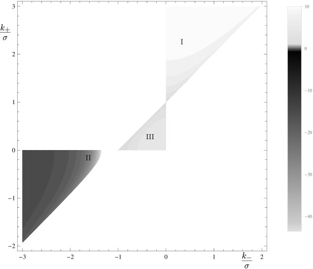
Figure 2: Contour plot of $\mathcal{P}H^{2}/(|\sigma|M^{d})$ as a function of $k_{-}/\sigma$, $k_{+}/\sigma$ at $\xi_{h}=0.3$. The regions I–III correspond to the allowed regions in the parameter space discussed in Sec. 2. In the region II (more dark), which corresponds to the negative visible brane tension, the radion is a ghost.

In the static limit (19) one has

$$\mathcal{P}=4dM^{d}\frac{k_{-}}{H^{2}r_{h}^{d-1}}\left(\frac{k_{+}}{r_{h}^{d-1}\triangle k}-1\right)^{-1}\,,$$

which, modulo notations, coincides with the result of Refs. [19, 22].

Up to the sign of $\mathcal{P}$, the action (62) coincides with the action for perturbations about a time-dependent background in a $(d+1)$-dimensional classical conformal theory. The latter theory is described by the action

$$S_{\varphi} = \int\limits d^{d+1}x\sqrt{-\gamma}\left[\frac{1}{2}\gamma^{\mu\nu}\partial_{\mu}\varphi\partial_{\nu}\varphi+\frac{{}^{(d+1)}R(d-1)}{8d}\varphi^{2}-\frac{(-\lambda^{2})}{2}\varphi^{\frac{2(d+1)}{d-1}}\right]$$ (63)

$$= \int\limits d^{d+1}x\left[\frac{1}{2}(\partial_{\mu}\tilde{\varphi})^{2}-\frac{(-\lambda^{2})}{2}\tilde{\varphi}^{\frac{2(d+1)}{d-1}}\right]\,,$$

with $\gamma_{\mu\nu}=a^{2}\eta_{\mu\nu}$, $\tilde{\varphi}=a^{\frac{d-1}{2}}\varphi$, while the background time-dependent solution is, at $\tau<0$,

$$\tilde{\varphi}_{c}=\left(\frac{d-1}{2\lambda}\right)^{\frac{d-1}{2}}\frac{1}{(-\tau)^{\frac{d-1}{2}}}\;.$$

Modulo the replacement of the real field $\varphi$ by complex one, eq. (63) is precisely the action considered in the context of (pseudo)conformal Universe model [1, 5].

The equation of motion for the canonicaly normalized radion $\phi$ obtained from the action (62), is

$$\Box\phi-\frac{(d+1)(d+3)}{4\tau^{2}}\phi=0\,.$$

Its negative frequency solution that tends to properly normalized mode of free quantum field as $p\tau\to-\infty$ is

$$\phi=\frac{\sqrt{-\tau}}{2^{\frac{d+2}{2}}\pi^{\frac{d-1}{2}}}\mathrm{e}^{\frac{i\pi}{4}(d-5)}H^{(1)}_{\frac{d+2}{2}}(-p\tau)\mathrm{e}^{i\mathbf{px}}\,.$$

At late times, when $-p\tau\ll 1$, one has

$$\phi=\mathrm{e}^{i\mathbf{kx}}\cdot\mathrm{e}^{\frac{i\pi}{4}(d+1)}\Gamma\left(\frac{d+2}{2}\right)\frac{1}{\pi^{\frac{d+1}{2}}p^{\frac{d+2}{2}}(-\tau)^{\frac{d+1}{2}}}\,,$$

what leads to the red power spectrum (2).

7.2 Radion-matter coupling

Let $T_{AB}^{\pm}$ and $\mathcal{T}_{\mu\nu}$ be the energy-momentum tensors of matter residing in the bulk and on the visible brane, respectively. $T_{AB}^{\pm}$ does not include contributions from the bulk cosmological constants and can be, in general, different in the different regions, while $\mathcal{T}_{\mu\nu}$ does not include the brane tension. We assume that the matter energy-momentum tensors are small and treat them as perturbations. For simplicity we also assume that there is no matter residing on the hidden brane. To derive the radion equation of motion in the presence of matter we note that in this case eqs. (37) and (34b) take the form

$${}^{(d+1)}R-(K_{\mu\nu}^{\pm(v)}K_{\pm(v)}^{\mu\nu}-K_{\pm}^{2})-k_{\pm}^{2}d(d+1)-\frac{n_{A}n_{B}T^{AB}_{\pm}}{M^{d}}=0\,,$$

$$\triangle K_{\mu\nu}^{(v)}=-\sigma\gamma_{\mu\nu}^{(v)}+\frac{1}{2M^{d}}\left(\mathcal{T}_{\mu\nu}-\frac{\gamma_{\mu\nu}\gamma^{\lambda\rho}\mathcal{T}_{\lambda\rho}}{d}\right)\,.$$

To the leading order in perturbations about the source-free background, one has from these equations

$${}^{(d+1)}R+d(d+1)\mathrm{s}_{\pm}^{2}k^{2}_{\pm}-2d\mathrm{c}_{\pm}k_{\pm}\delta K_{\pm}-\frac{H^{2}T_{\xi\xi}^{\pm}}{M^{d}}=0\,,$$

$$\triangle\delta K=-\frac{H^{2}\tau^{2}\mathcal{T}}{2dM^{2}}\,,$$

where $\mathcal{T}\equiv\eta^{\mu\nu}\mathcal{T}_{\mu\nu}$. We actually have three equations, which can be used to find the induced scalar curvature ${}^{(d+1)}R$ and the values of $\delta K_{\pm}$ on both sides of the visible brane. The result for $\delta K_{\pm}$ is

$$\delta K_{\pm}=\frac{1}{2dM^{d}\sigma}\left(\mathrm{c}_{\mp}k_{\mp}H^{2}\tau^{2}\mathcal{T}-H^{2}\triangle T_{\xi\xi}\right)\,.$$ (64)

To proceed, we make use of eq. (36). The quantity $h^{\prime}(0)$ entering that equation can be found by using eq. (28h) which takes the following form in the presence of matter:

$$-\mathfrak{s}\left(\frac{h^{\prime}}{\mathfrak{s}}\right)^{\prime}=\frac{1}{M^{d}}\left(T_{\xi\xi}+\frac{T}{dk^{2}\mathfrak{s}^{2}}\right)\,,$$

where $T\equiv g^{AB}T_{AB}$. Integrating this equation with the boundary condition (32) and plugging the result into eq. (36) and then into eq. (64), one finally arrives at the desired equation of motion for the canonically normalized radion (60),

$$\Box\phi-\frac{(d+1)(d+3)}{4\tau^{2}}\phi=$$

$$\sqrt{\frac{{|\mathcal{P}|H^{2}}}{4M^{2d}|H\tau|^{d-1}}}\left[\frac{1}{d\sigma}\left(\mathrm{c}_{+}k_{+}\mathcal{T}-\frac{\triangle T_{\xi\xi}}{\tau^{2}}\right)+\frac{1}{\tau^{2}}\int\limits_{-\xi_{h}}^{0}\frac{d\xi}{\mathfrak{s}_{-}k_{-}}\left(T_{\xi\xi}^{-}+\frac{T^{-}}{dk_{-}^{2}\mathfrak{s}_{-}^{2}}\right)\right]\,.$$ (65)

This reiterates that the radion has unsuppressed coupling to matter residing on the visible brane. Equation (65) shows also that the radion does not interact with matter residing in the “+” region outside the visible brane. The latter property is consistent with the fact that the non-trivial part of the radion wave function is concentrated on and between the branes, see the discussion after eq. (55).

7.3 Graviton effective action

In the same way one gets the graviton effective action

$$S_{TT}=\frac{M_{\mathrm{Pl}}^{d-1}}{4}\int\limits dx^{d+1}\frac{(\partial_{\mu}h_{(d/2)ij}^{TT})^{2}}{|H\tau|^{d-1}}\,,$$

with $(d+1)$-dimensional Planck mass

$$M_{\mathrm{Pl}}^{d-1}=2M^{d}H^{d-1}\int\limits_{-\xi_{h}}^{\infty}\frac{d\xi}{k^{d}\mathfrak{s}^{d}}\,,$$ (66)

where we have set $\beta_{\frac{d}{2}}^{2}=1$ which is appropriate from the viewpoint of a $(d+1)$-dimensional observer localized on the visible brane (see the discussion in Ref. [17]). In the static limit (19), the $(d+1)$-dimensional Planck mass is

$$M_{\mathrm{Pl}}^{d-1}=\frac{1}{r_{h}^{d-1}k_{-}(d-1)}\left(1-r_{h}^{d-1}\frac{\triangle k}{k_{+}}\right)\,.$$

This agrees with Ref. [20].

7.4 Limit of single visible brane

7.4.1 $k_{-}>0$

In the case $k_{-}>0$, the adS boundary is located at $-\xi_{-}<-\xi_{h}<0$ and the hidden brane can be pushed to it, $\xi_{h}\to\xi_{-}$. In this limit one has

$$\mathcal{P}=4d(d+1)\frac{M^{d}}{H}\left((d+1)\frac{k_{+}\mathrm{c_{+}}}{k_{-}\mathrm{c}_{-}}\frac{H}{\sigma}+\left(\frac{\mathrm{s_{-}}}{\mathrm{c_{-}}}\right)^{3}F\left(1,\frac{3}{2};\frac{d+3}{2};\frac{\mathrm{s}_{-}^{2}}{\mathrm{c}_{-}^{2}}\right)\right)^{-1}\,.$$

This is finite and, therefore, the radion does not decouple from the physical spectrum. The radion-matter coupling (65) is finite as well. On the other hand, the integral (66) that yields the effective Planck mass, diverges and hence the graviton does not interact with matter and decouples.

7.4.2 $k_{-}<0$

In the opposite case $k_{-}<0$ the adS boundary is absent ($\xi_{-}<0$) and the single brane limit corresponds to $\xi_{h}\to\infty$. In that case only the last term in the expression for the radion wave function in the “$-$” domain (53) survives. The radion becomes pure gauge, and hence unphysical, in both domains. One can also see that in the limit $\xi_{h}\to\infty$, $\mathcal{P}$ vanishes. So, the radion does not couple to matter, as it should be.

On the contrary, the effective Planck mass (66) is finite and graviton is the only light physical degree of freedom.

8 Conclusion

To conclude, in this paper we have performed the analysis of the linearized metric perturbations in the dynamical Lykken-Randall type model. We have derived equations of motion for the scalar, vector and tensor modes and have shown that, in general, the radion and graviton are the only light modes. However, in the single brane regime, depending on the behaviour of the warp factor in the “$-$” region, graviton or radion decouples from the physical spectrum: if the warp factor grows outward the visible brane ($k_{-}>0$) and there is the adS boundary, only the radion is present in the physical spectrum while the graviton decouples, and vise versa in the opposite case. We have also shown that if the visible brane has negative tension, the radion is a ghost. Although these features of the metric perturbations are interesting by themselves, we think our main result is the radion equation of motion. This equation leads to the red power spectrum, as one could have anticiated from the holographic picture. This means that the potentially observable features of the (pseudo)conformal Universe  [5] hold also for the de Sitter brane moving in the adS background.

Appendix A Spectrum of the operator (44)

Let us find the spectrum of eigenvalues $\kappa^{2}$ in eq. (44). The eigenfunctions $\beta_{\kappa}$ and their first derivatives must be continuous across the visible brane and obey $\beta_{\kappa}^{\prime}(-\xi_{h})=0$ at the hidden brane.

We multiply eq. (44) by $\beta_{\kappa}^{*}$, integrate the result with the measure $1/(k\mathfrak{s})^{d}$, and, taking into account the boundary conditions, obtain

$$\int\limits_{-\xi_{h}}^{\infty}\frac{d\xi}{(k\mathfrak{s})^{d}}|\beta_{\kappa}^{\prime}|^{2}=\int\limits_{-\xi_{h}}^{\infty}\frac{d\xi}{(k\mathfrak{s})^{d}}\left(\frac{d^{2}}{4}-\kappa^{2}\right)|\beta_{\kappa}|^{2}\,,$$

which shows that $\kappa^{2}\leq d^{2}/4$. As we will see, the spectrum is continuous at $\kappa^{2}\leq 0$. At $\kappa=d/2$, there is the constant mode (45). We will argue that the latter mode disappears for $k_{-}>0$ and $\xi_{h}\to\xi_{-}$, that is, when the hidden brane is pushed to the adS boundary.

There may exist solutions with

$$d^{2}/4>\kappa^{2}>0\,.$$

Our main purpose here is to demonstrate that, in fact, there are no such solutions. To this end we introduce the wave function

$$\tilde{\beta}_{\kappa}(\xi)=\beta_{\kappa}(\xi)(k\mathfrak{s})^{-d/2}$$

and cast eq. (44) into the form of the Schrödinger equation

$$-\partial_{\xi}^{2}\tilde{\beta}_{\kappa}+\left(\frac{d(d+2)}{4\mathfrak{s}^{2}}-\frac{d\sigma}{2H}\delta(\xi)\right)\tilde{\beta}_{\kappa}=-\kappa^{2}\tilde{\beta}_{\kappa}\,,$$ (67)

where the appearance of $\delta(\xi)$ is due to the continuous matching conditions for $\beta_{\kappa}$ on the visible brane which translates to the following conditions for $\tilde{\beta}_{\kappa}$,

$$\triangle\tilde{\beta}_{\kappa}=0\,,\ \ \ \ \triangle\tilde{\beta}^{\prime}_{\kappa}=-\frac{d\sigma}{2H}\tilde{\beta}_{\kappa}\,.$$ (68)

The boundary condition on the hidden brane (32) takes the following form,

$$\tilde{\beta}^{\prime}_{\kappa}+\frac{d\mathrm{c}_{h}}{2\mathrm{s}_{h}}\tilde{\beta}_{\kappa}=0\,,$$ (69)

and $\tilde{\beta}_{\kappa}$ should be normalizable with unit measure:

$$\int\limits_{-\xi_{h}}^{\infty}d\xi\tilde{\beta}_{\kappa^{\prime}}^{*}\tilde{\beta}_{\kappa}=\delta_{\kappa^{\prime},\kappa}\,,$$ (70)

where $\delta_{\kappa^{\prime},\kappa}=\delta(\kappa^{\prime}-\kappa)$ for the modes belonging to the continuous part of the spectrum.

To warm up, let us demonstrate that at $\kappa^{2}<0$ the spectrum is continuous. In general, in the “$-$” region, there always exist two linear independent solutions to eq. (67), and hence one can construct unique solution (up to an overall constant) $\tilde{\beta}_{\kappa}^{<}$ to eq. (67) satisfying the boundary condition (69) on the hidden brane. At large $\xi>0$, the potential term in eq. (67) can be neglected and at $\kappa^{2}<0$ there are two oscillating solutions $\sim\mathrm{e}^{\pm i|\kappa|\xi}$. A linear combination of them can be chosen to satisfy eq. (68) (at any $\kappa^{2}<0$) and to match $\tilde{\beta}_{\kappa}^{<}$. Thus, the spectrum is indeed continuous at $\kappa^{2}<0$. This argument does not apply to the special case $\kappa=0$ when the asymptotic behaviour of the two solutions at $\xi\to\infty$ is $\mathrm{const}\neq 0$ and $\xi$, since only the first one is suitable. In any case, if $\tilde{\beta}_{0}$ exists then it belongs to the continuous part of the spectrum.

To see that the boundary value problem (67) – (70) has only one discrete solution, we note that the first term in parenthesis in eq. (67) is always positive $V\propto 1/\mathfrak{s}^{2}>0$. Let us turn off this term. Then we deal with a particle in the $\delta$-function well. It is straightforward to check that the spectrum in that case consists of one negative discrete level and continuous part starting from zero. Switching on $V$ in (67) can only lead to a non-negative addition to each eigenvalue. Since the continuous parts coincide in both cases (vanishing and nonvanishing $V$) this means that non-zero potential may lead to the disappearance of the negative discrete level, but it cannot lead to the appearance of the second negative discrete level. Therefore, the boundary value problem (67) – (70) can have only one discrete level and, indeed, it has the level with $\kappa=d/2$.

Let us consider the case of the single visible brane. In general, there are two different cases: $k_{-}\leq 0$ ($\xi_{-}\leq 0$) and $k_{-}>0$ ($\xi_{-}>0$). In the first case the boundary condition on the hidden brane (69) is replaced by the normalization condition (70) with $\xi_{h}\to-\infty$. It is straightforward to see that all above arguments are still in force in that case. So, the spectrum consists of the discrete level with $\kappa=d/2$ and continuous part starting from zero.

In the case $k_{-}>0$ one replaces $\xi_{h}\to\xi_{-}$ and the boundary condition (69) becomes

$$\tilde{\beta}_{\kappa}(-\xi_{-})=0\,,$$

that is, the wave functions vanish at the adS boundary, and the above arguments do not work. Let us argue that there are no discrete levels in this case.

Suppose that there exists a discrete level. The corresponding wave function, being the wave function of the ground state, has no nodes and can be chosen to be positive everywhere. Then, integrating eq. (67) and taking into account the boundary and matching conditions, one obtains the following inequality,

$$\frac{d\sigma}{2H}\tilde{\beta}_{\kappa}(0)=\int\limits_{-\xi_{-}}^{\infty}d\xi\left(\frac{d(d+2)}{4\mathfrak{s}^{2}}+\kappa^{2}\right)\tilde{\beta}_{\kappa}>\int\limits_{0}^{\infty}d\xi\frac{d(d+2)}{4\mathfrak{s}^{2}_{+}}\tilde{\beta}_{\kappa}\,.$$ (71)

Let us consider two extreme cases: a) $\xi_{+}\ll 1$ and b) $\xi_{+}\gg 1$. The first case (see (17)) corresponds to slowly expanding brane, $H/k_{+}\ll 1$, and hence $\xi_{+}\simeq H/k_{+}$. In that case the integral in the right hand side of eq. (71) is saturated near the origin and is proportional to $1/\xi_{+}$:

$$\frac{d\sigma}{2H}\tilde{\beta}_{\kappa}(0)>\frac{d(d+2)}{4}\frac{1}{\xi_{+}}\tilde{\beta}_{\kappa}(0)=\frac{d(d+2)}{4}\frac{k_{+}}{H}\tilde{\beta}_{\kappa}(0)\,,$$

or

$$1>\frac{(d+2)}{2}\frac{k_{+}}{\sigma}\,.$$

This contradicts the relation $k_{+}>\sigma$ which follows from (15). Hence, there is no discrete level in that case.

The opposite case $\xi_{-}>\xi_{+}\gg 1$ corresponds to rapidly expanding brane, $H\gg k_{\pm},\sigma$. In that case

$$\xi_{\pm}\simeq\log\left(\frac{2H}{k_{\pm}}\right)\,,$$ (72)

and the first term in parenthesis in eq. (67) can be neglected. Indeed, in the “$+$” region this approximation is valid at all $\xi$, while in the “$-$” region the approximation may only decrease the value of $\kappa^{2}$. Then, solving eqs. (67), (68) with vanishing potential, one finds

$$\kappa=\frac{d\sigma}{4H}\left(1-\mathrm{e}^{-2\xi_{-}\kappa}\right)\simeq\frac{d\sigma}{4H}\ll 1\,,$$

$$\tilde{\beta}_{\kappa}(\xi>0)=\tilde{\beta}_{\kappa}(0)\mathrm{e}^{-\kappa\xi}\,.$$ (73)

By substituting (72), (73) into (71) one obtains

$$1>\frac{(d+2)}{2}\frac{k_{+}^{2}}{H\sigma(2+\kappa)}\simeq\frac{(d+2)}{4}\frac{k_{+}^{2}}{H\sigma}>\frac{d+2}{2}\,,$$

where we have used (16) and inequality

$$((k_{+}+k_{-})^{2}-\sigma^{2})((k_{+}-k_{-})^{2}-\sigma^{2})<(k_{+}+k_{-})^{2}(k_{+}-k_{-})^{2}\leq k_{+}^{4}\,.$$

Thus, we again come to contradiction and the discrete level is absent.

Another way to see that the discrete level is absent is to consider what happens with the mode $\kappa=d/2$ in the limit $\xi_{h}\to-\xi_{-}$. In this limit the normalized mode has the form,

$$\tilde{\beta}_{\frac{d}{2}}(\xi)=\sqrt{d-1}(\xi_{-}-\xi_{h})^{\frac{d-1}{2}}\frac{k_{-}^{\frac{d}{2}}}{(k\mathfrak{s})^{\frac{d}{2}}}\,,$$ (74)

where we have used the fact that the corresponding normalization integral is saturated at $\xi\to\xi_{h}$:

$$\int\limits_{-\xi_{h}\to-\xi_{-}}^{\infty}\frac{d\xi}{(k\mathfrak{s})^{d}}\simeq\frac{1}{(d-1)k_{-}^{d}(\xi_{-}-\xi_{h})^{d-1}}\,.$$

As we have discussed above at any $\xi_{h}\neq\xi_{-}$ the mode (74) is the only discrete mode in the spectrum. It follows from (74) that at any given $\xi>\xi_{-}$ this mode tends to zero in the limit $\xi_{h}\to\xi_{-}$ and, therefore, does not contribute to any observable in the whole space except for an infinitesimal region near the adS boundary.

To summarize, we have seen that the spectrum of the operator (44) defined on the class of continuous functions in the case of two branes as well as in the case of single brane and $k_{-}\leq 0$ consits of one discrete level with $\kappa=d/2$ ($\nu=1-d$) and continuous part starting from $\kappa=0$, $\nu=(d-2)^{2}/4$. In the case of single brane and $k_{-}>0$ the discrete level is absent, the spectrum is continuous and starts from $\kappa=0$, $\nu=(d-2)^{2}/4$.

References

- [1] V. A. Rubakov, JCAP 0909 (2009) 030 [arXiv:0906.3693 [hep-th]].
- [2] P. Creminelli, A. Nicolis and E. Trincherini, JCAP 1011 (2010) 021 [arXiv:1007.0027 [hep-th]].
- [3] K. Hinterbichler and J. Khoury, JCAP 1204 (2012) 023 [arXiv:1106.1428 [hep-th]].
- [4] K. Hinterbichler, A. Joyce, J. Khoury and G. E. J. Miller, JCAP 1212 (2012) 030 [arXiv:1209.5742 [hep-th]].
- [5] M. Libanov, V. Rubakov and G. Rubtsov, JETP Lett. 102 (2015) 561 [arXiv:1508.07728 [hep-th]].
- [6] M. Osipov and V. Rubakov, JETP Lett. 93 (2011) 52 [arXiv:1007.3417 [hep-th]].
- [7] M. Libanov, S. Ramazanov and V. Rubakov, JCAP 1106 (2011) 010 [arXiv:1102.1390 [hep-th]].
- [8] P. Creminelli, A. Joyce, J. Khoury and M. Simonovic, JCAP 1304 (2013) 020 [arXiv:1212.3329].
-
[9]
M. Libanov, S. Mironov and V. Rubakov,
Phys. Rev. D 84 (2011) 083502
[arXiv:1105.6230 [astro-ph.CO]];
M. Libanov, S. Mironov and V. Rubakov, Prog. Theor. Phys. Suppl. 190 (2011) 120 [arXiv:1012.5737 [hep-th]];
S. A. Mironov, S. R. Ramazanov and V. A. Rubakov, JCAP 1404 (2014) 015 [arXiv:1312.7808 [astro-ph.CO]]. -
[10]
M. Libanov and V. Rubakov,
JCAP 1011 (2010) 045
[arXiv:1007.4949 [hep-th]];
M. V. Libanov and V. A. Rubakov, Theor. Math. Phys. 170 (2012) 151 [Teor. Mat. Fiz. 170 (2012) 188]. -
[11]
S. R. Ramazanov and G. I. Rubtsov,
JCAP 1205 (2012) 033
[arXiv:1202.4357 [astro-ph.CO]];
S. R. Ramazanov and G. Rubtsov, Phys. Rev. D 89 (2014) no.4, 043517 [arXiv:1311.3272 [astro-ph.CO]];
G. I. Rubtsov and S. R. Ramazanov, Phys. Rev. D 91 (2015) 043514 [arXiv:1406.7722 [astro-ph.CO]]. - [12] K. Hinterbichler, A. Joyce and J. Khoury, JCAP 1206 (2012) 043 [arXiv:1202.6056 [hep-th]].
- [13] K. Hinterbichler, J. Stokes and M. Trodden, JHEP 1501 (2015) 090 [arXiv:1408.1955 [hep-th]].
- [14] M. Libanov, V. Rubakov and S. Sibiryakov, Phys. Lett. B 741 (2015) 239 [arXiv:1409.4363 [hep-th]].
- [15] M. Libanov and V. Rubakov, Phys. Rev. D 91 (2015) 103515 [arXiv:1502.05897 [hep-th]].
- [16] V. A. Rubakov, Phys. Usp. 44 (2001) 871 [Usp. Fiz. Nauk 171 (2001) 913] [hep-ph/0104152].
- [17] L. Randall and R. Sundrum, Phys. Rev. Lett. 83 (1999) 3370 [hep-ph/9905221].
- [18] C. Charmousis, R. Gregory and V. A. Rubakov, Phys. Rev. D 62 (2000) 067505 [hep-th/9912160].
- [19] L. Pilo, R. Rattazzi and A. Zaffaroni, JHEP 0007 (2000) 056 [hep-th/0004028].
- [20] J. Lykken and L. Randall, JHEP 06 (2000) 014 [hep-th/9908076].
- [21] R. Gregory, V. A. Rubakov and S. M. Sibiryakov, Phys. Rev. Lett. 84 (2000) 5928 [hep-th/0002072].
- [22] S. L. Dubovsky and M. V. Libanov, JHEP 0311 (2003) 038 [hep-th/0309131].
- [23] P. Kraus, JHEP 9912 (1999) 011 [hep-th/9910149].
- [24] D. Ida, JHEP 0009 (2000) 014 [gr-qc/9912002].
- [25] M. Cvetic and J. Wang, Phys. Rev. D 61 (2000) 124020 [hep-th/9912187].
- [26] S. Mukohyama, T. Shiromizu and K. i. Maeda, Phys. Rev. D 62 (2000) 024028 Erratum: Phys. Rev. D 63 (2001) 029901 [hep-th/9912287].
- [27] P. Bowcock, C. Charmousis and R. Gregory, Class. Quant. Grav. 17 (2000) 4745 [hep-th/0007177].
- [28] D. S. Gorbunov, V. A. Rubakov and S. M. Sibiryakov, JHEP 0110 (2001) 015 [hep-th/0108017].
- [29] U. Gen and M. Sasaki, Prog. Theor. Phys. 105 (2001) 591 [gr-qc/0011078].
- [30] P. Binetruy, C. Deffayet and D. Langlois, Nucl. Phys. B 615 (2001) 219 [hep-th/0101234].
- [31] Z. Chacko and P. J. Fox, Phys. Rev. D 64 (2001) 024015 [hep-th/0102023].
- [32] U. Gen and M. Sasaki, Prog. Theor. Phys. 108 (2002) 471 [gr-qc/0201031].
- [33] T. Chiba, Phys. Rev. D 62 (2000) 021502 doi:10.1103/PhysRevD.62.021502 [gr-qc/0001029].
- [34] W. Israel, Nuovo Cim. B 44S10 (1966) 1 [Nuovo Cim. B 44 (1966) 1] Erratum: Nuovo Cim. B 48 (1967) 463.
- [35] V. A. Berezin, V. A. Kuzmin and I. I. Tkachev, Phys. Rev. D 36 (1987) 2919.