Relating information entropy and mass variance to measure bias and non-Gaussianity

Abstract

We relate the information entropy and the mass variance of any distribution in the regime of small fluctuations. We use a set of Monte Carlo simulations of different homogeneous and inhomogeneous distributions to verify the relation and also test it in a set of cosmological N-body simulations. We find that the relation is in excellent agreement with the simulations and is independent of number density and the nature of the distributions. We show that the relation between information entropy and mass variance can be used to determine the linear bias on large scales and detect the signatures of non-Gaussianity on small scales in galaxy distributions.

1 Introduction

Understanding the formation and evolution of the large scale structures in the Universe is one of the most complex issues in cosmology. The galaxies are the basic building blocks of the large scale structures and their spatial distribution reveals how the luminous matter is distributed in the Universe. The study of the distribution of galaxies is one of the most direct probe of the large scale structures. The modern galaxy redshift surveys like the Sloan Digital Sky Survey (SDSS) (York et al., 2000) has now mapped the distribution of more than a million galaxies and quasars which provides the most detailed three-dimensional maps of the Universe ever made in the history of mankind. The maps reveal that the galaxies are distributed in an interconnected complex filamentary network namely the cosmic web. The cosmic web emerges naturally from the gravitational amplifications of the primordial density fluctuations seeded in the early universe. The distribution of galaxies in the cosmic web encodes a wealth of information about the formation and evolution of the large scale structures. A large number of statistical tools have been developed so far to quantify the galaxy distribution and unravel the large scale structures. The correlation functions (Peebles, 1980) characterize the statistical properties of the galaxy distributions. The two-point correlation function and its Fourier space counterpart, the power spectrum remain some of the most popular measure of galaxy clustering todate. These statistics provide a complete description for the primordial density perturbations which are assumed to be Gaussian in the linear regime. But in subsequent stages of non-linear gravitational evolution, the phase coupling of the Fourier modes produces non-vanishing higher-order correlation functions and polyspectra. In principle a full hierarchy of N-point statistics is required to provide a complete description of the distribution. The void probability function (White, 1979) provides a characterization of voidness that combine many higher moments of the distribution. Other methods to quantify the cosmic web includes the percolation analysis (Shandarin & Zeldovich, 1983; Einasto et al., 1984), the genus statistics (Gott, Dickinson, & Melott, 1986), the minimal spanning tree (Barrow et al., 1985)), the Voronoi tessellation (Icke & van de Weygaert, 1987; van de Weygaert & Icke, 1989), the Minkowski functionals (Mecke et al., 1994; Schmalzing & Buchert, 1997), the Shapefinders (Sahni, Sathyaprakash,& Shandarin, 1998), the critical point statistics (Colombi, Pogosyan & Souradeep, 2000), the marked point process (Stoica et al., 2005), the multiscale morphology filter (Aragón-Calvo et al., 2007), the skeleton formalism (Sousbie et al., 2008) and the local dimension (Sarkar & Bharadwaj, 2009).

The popularity of the two-point correlation function and the power spectrum lies in the fact that they can be easily measured and related to the theories of structure formation whereas it is hard to do so for most of the other statistics. The variance of the mass distribution smoothed with a sphere of radius $r$ is a simple and powerful statistical measure which is directly related to the power spectrum. Information entropy is a statistical measure which can help us to study the formation and evolution of structures from an information theoretic viewpoint. Recently information entropy has been used as a measure of homogeneity (Pandey, 2013; Pandey & Sarkar, 2015, 2016) and isotropy (Pandey, 2016) of the Universe. Both the information entropy and the mass variance can be used as a measure of the non-uniformity of a probability distribution. The entropy uses more information about the probability distribution as it is related to the higher order moments of a distribution. The variance can be treated as an equivalent measure only when the probability distribution is fully described by the first two moments such as in a Gaussian distribution. However a highly tailed distribution is not uniquely determined even by its all the higher order moments (Patel, Kapadia & Owen, 1976; Romano & Siegel, 1986; Carron, 2011; Carron & Neyrinck, 2012).

Different statistical tools have been designed to explore different aspects of the galaxy distribution and when possible it is important to relate these statistical measures for a better interpretation of different cosmological observations. In future, Information theory can find many potential applications in cosmology. It would be highly desirable to relate the information entropy to the other conventional measures such as the mass variance and the power spectrum. In this paper we particularly explore the relation between the discrete Shannon entropy and the mass variance of a distribution and test it using N-body simulations and the Monte Carlo simulations of different distributions.

We also explore a few possible applications of this relation in cosmology particularly to constrain the large-scale linear bias and non-Gaussianity in galaxy redshift surveys. Galaxies are known to be a biased tracer of the underlying dark matter distribution. Currently there exist several methods to determine the large scale linear bias. The bias can be directly determined from the two-point correlation function and power spectrum (Norberg et al., 2001; Tegmark et al., 2004; Zehavi et al., 2011), the three-point correlation function and bispectrum (Feldman et al., 2001; Verde et al., 2002; Gaztañaga et al., 2005), the redshift space distortion parameter $\beta=\Omega_{m}^{0.6}/b$ (Hawkins et al., 2003; Tegmark et al., 2004) and the filamentarity of the galaxy distribution (Bharadwaj & Pandey, 2004; Pandey & Bharadwaj, 2007). We employ the information entropy-mass variance relation to propose a new method which can be used to determine the large scale linear bias from galaxy redshift surveys.

Non-Gaussianity of the cosmic density field is one of the most interesting issues in cosmology. In the current paradigm, the primordial density fluctuations are assumed to be Gaussian and signatures of non-Gaussianities in these fluctuations can be used to constrain different inflationary models in cosmology (Bartolo et al., 2004). As the density fluctuations grow, the probability distribution function of the cosmic density field develope extended tails in the overdense regions and gets truncated in the underdense regions. These non-Gaussianities induced by the structure formation are much stronger and dominates any primordial non-Gaussianities from the early Universe. In the present work we do not address the primordial non-Gaussianities but the non-Gaussianties introduced by the nonlinear evolution of the cosmic density field. We investigate if the information entropy-mass variance relation can be used to detect the signatures of non-Gaussianity in the galaxy distribution.

A brief outline of the paper follows. In section 2 we describe the relation between information entropy and mass variance followed by a discussion on some possible applications of this relation in section 3. We describe the data in section 4 and finally present the results and conclusions in section 5.

2 Information entropy and cosmological mass variance

Information entropy (Shannon, 1948) is a measure in Information theory which quantify the amount of information required to describe a random variable. According to Shannon, the information contained in any outcome of a probabilistic process is given by $I(p(x_{i}))=\log\frac{1}{p(x_{i})}$ where $p(x_{i})$ is the probability of that particular outcome. If there are $n$ outcomes of the random variable $x$ given by $\{x_{i}:i=1,....n\}$ and $N$ observations are made then we expect $N\,p(x_{i})$ occurrences for each of the outcome $x_{i}$. The average information required to describe the discrete random variable $x$ is then given by the information entropy $H(x)$ defined as,

$$H(x) = \frac{1}{N}\sum^{n}_{i=1}N\,p(x_{i})\,\log\frac{1}{p(x_{i})}$$

$$= -\sum^{n}_{i=1}\,p(x_{i})\,\log\,p(x_{i})$$

We consider a three dimensional distribution of $N$ points in a finite region of space. We place a measuring sphere of radius $r$ centered at each point in the distribution and count the number of other points $n_{i}(<r)$ within the sphere. Only the centers for which the measuring spheres lie completely within the spatial boundary of the region are considered. To ensure this, we discard all the centers which reside within a distance $r$ from the boundary. Evidently the number of centers $M(r)$ available at radius $r$, would decrease with increasing $r$ for any finite volume. We consider the subset of all the points which are residing in the $M(r)$ spheres available at any particular radius $r$. If a point is randomly drawn out of this subset the random point is expected to reside in one or multiple of these spheres with different probabilities each given by, $f_{i,r}=\frac{\rho_{i,r}}{\sum^{M(r)}_{i=1}\,\rho_{i,r}}$ with the constraint $\sum^{M(r)}_{i=1}\,f_{i,r}=1$. Here $\rho_{i,r}=\frac{n_{i}(<r)}{\frac{4}{3}\pi r^{3}}$ is the density at the $i^{th}$ center. We consider this experiment at each radius $r$ and label the outcome with a random variable $x_{r}$ for radius $r$.

The random variable $x_{r}$ has the information entropy,

$$H_{r} = -\sum^{M(r)}_{i=1}\,f_{i,r}\,\log\,f_{i,r}$$ (2)

$$= \log(\sum^{M(r)}_{i=1}n_{i}(<r))-\frac{\sum^{M(r)}_{i=1}\,n_{i}(<r)\,\log(n_{i}(<r))}{\sum^{M(r)}_{i=1}\,n_{i}(<r)}$$

where the base of the logarithm is $10$. It may be noted here that the choice of the base is arbitrary and different choices would only result in different units for entropy.

The values of $f_{i,r}$ become $\frac{1}{M(r)}$ for all the centres when the randomly drawn point has the same probability to appear in any of the $M(r)$ spheres. This maximizes the entropy of $x_{r}$ to $(H_{r})_{max}=\log\,M(r)$. The maximum entropy corresponds to maximum uncertainty in the location of the randomly drawn point. The quantity $(H_{r})_{max}-H_{r}$ at any $r$ quantifies the deviation of the entropy from its maximum value. We are interested to relate this statistical measure to other conventional measures of large scale structures. We calculate $(H_{r})_{max}-H_{r}$ for a distribution with small fluctuations in the number density. We write the number counts in Equation 2 as $n_{i}(<r)=n_{0}(<r)+\delta n_{i}(<r)$, where $n_{0}(<r)$ is the mean number counts in spheres of radius $r$ and $\delta n_{i}(<r)$ is the fluctuations around the mean. We expand the $\log(1+\frac{\delta n_{i}(<r)}{n_{0}(<r)})$ terms in Taylor series as $\frac{\delta n_{i}(<r)}{n_{0}(<r)}<1$. Keeping terms upto third order and simplifying the expression we get,

$$(H_{r})_{max}-H_{r}\,=\,\frac{1}{2\,M(r)\,n_{0}(<r)^{2}}\sum^{M(r)}_{i=1}\delta n_{i}^{2}(<r)$$

$$-\frac{1}{6\,M(r)\,n_{0}(<r)^{3}}\sum^{M(r)}_{i=1}\delta n_{i}^{3}(<r)$$

$$+\frac{1}{3\,M(r)\,n_{0}(<r)^{4}}\sum^{M(r)}_{i=1}\delta n_{i}^{4}(<r)-...$$ (3)

The variance is a conventional measure of the non-uniformity present in a distribution and it is widely used in cosmology. For example one can estimate the mass variance of the smoothed density field from the power spectrum of the density field.

$$\sigma_{r}^{2}\,=\,\frac{1}{(2\,\pi)^{2}}\,\int_{0}^{\infty}k^{2}P(k){W(kr)}^{2}dk$$ (4)

where, $r$ is the size of the spherical top hat filter, $P(k)$ is the power spectrum and $W(kr)=3\frac{\sin(kr)-kr\cos(kr)}{(kr)^{3}}$ is the Fourier transform of the top-hat window function.

Alternatively one can also estimate the normalized mass variance of the 3D distribution by simply using the number counts and assuming equal mass for all the particles. The normalized mass variance in this case is given by,

$$\sigma_{r}^{2}=\frac{\overline{n^{2}(<r)}-(\bar{n}(<r))^{2}}{(\bar{n}(<r))^{2}}$$ (5)

Here the bars denote average of the respective quantities over the $M(r)$ spheres available at radius $r$.

Rewriting the number counts in Equation 5 as $n_{i}(<r)=n_{0}(<r)+\delta n_{i}(<r)$ and simplifying we get,

$$\sigma_{r}^{2}\,=\,\frac{1}{\,M(r)\,n_{0}(<r)^{2}}\sum^{M(r)}_{i=1}\delta n_{i}^{2}(<r)$$ (6)

We see from Equation 3 and Equation 6 that there is no direct relationship between the entropy and the mass variance. However in the limit of small fluctuations i.e. when $\frac{\delta n_{i}(<r)}{n_{0}(<r)}<<1$, one can drop the higher order terms in Equation 3 to relate entropy with variance as,

$$(H_{r})_{max}-H_{r}\,=\,\frac{\sigma_{r}^{2}}{2}$$ (7)

It may be noted here that in the numerical calculations of entropy using Equation 2 we chose the base of the logarithm to be $10$ whereas the analytical expression obtained in Equation 3 is based on the natural logarithm. So a factor of $\frac{1}{\log_{e}10}$ should be multiplied to the right hand side of Equation 3 and Equation 7 while comparing them with the numerical results from simulations.

The maximum entropy $(H_{r})_{max}$ at scale $r$ is not the same for different distributions as $M(r)$ varies differently with $r$ for different distributions. In the present scheme $M(r)$ can be written as,

$$M(r)=n_{0}\,\int_{0}^{R-r}(1+\xi(y))\,d^{3}y$$

$$=n_{0}\,V+4\pi n_{0}\int_{0}^{R-r}y^{2}\,\xi(y)\,dy$$ (8)

which is just the average number of points in a sphere of radius $R-r$. Here $R$ is the radius of the entire spherical sampling volume, $n_{0}$ is the mean density of the distribution, $\xi(y)$ is the two point correlation function and $V=\frac{4}{3}\pi(R-r)^{3}$ is the volume of the sphere hosting all the centers of the spheres having a radius $r$. Behaviour of $\xi(y)$ would be different for different distributions. Further Equation 8 would underestimate $M(r)$ if the higher order correlation functions are non-zero.

We numerically compute the information entropy for different distributions using Equation 2 and the mass variance for the same distributions using Equation 5 and compare them to test the validity of the relation given by Equation 7.

3 Bias and non-Gaussianity from the information entropy-mass variance relation

Using the information entropy-mass variance relation described in the previous section we propose a method for determining the large-scale linear bias of galaxy distributions from galaxy surveys. On large scales one can define the linear bias of galaxies by the ratio $b=\frac{\delta_{g}}{\delta_{m}}$, where $\delta_{g}$ and $\delta_{m}$ are the smoothed density contrast of galaxies and dark matter respectively. The power spectrum $P(k)$ is given by, $\langle\delta(\vec{k})\delta(\vec{k^{\prime}})\rangle=(2\pi)^{3}\delta_{D}^{3}(\vec{k}-\vec{k^{\prime}})\,P(k)$. So the power spectrum $P_{g}(k)$ of the galaxies would be $b^{2}$ times the power spectrum $P_{m}(k)$ of the dark matter on large scales. According to Equation 4, the mass variance of the galaxy distribution is also expected to be $b^{2}$ times the mass variance of the dark matter distribution on large scales. This immediately suggests that one can use the information entropy-mass variance relation (Equation 7) to determine the linear bias parameter on large scales. One needs simply the ratios of $(H_{r})_{max}-H_{r}$ for the galaxy distribution and dark matter distribution to determine the linear bias given by,

$$b=\sqrt{\frac{((H_{r})_{max}-H_{r})_{g}}{((H_{r})_{max}-H_{r})_{m}}}$$ (9)

The Equation 9 involves only the measurement of the information entropy from the galaxy distributions and the N-body simulations of the $\Lambda$CDM model. It may be noted here that in this method one can completely bypass the measurements of the power spectrum $P(k)$, the two-point correlation function $\xi(r)$ and the mass variance $\sigma_{r}^{2}$ of the associated distributions. The information entropy is relatively straightforward to compute compared to the power spectrum or the two-point correlation function. This provides a simple alternative method to determine the large-scale linear bias parameter from the measurements of information entropy alone.

Further the relation can be also used to study the evolution of clustering in the galaxy distribution by comparing the $(H_{r})_{max}-H_{r}$ measures at different redshifts. The shape of the power spectrum is preserved on large scales and its amplitude grows proportional to $D^{2}(t)$ and $b^{2}(t)$ where $D(t)$ is the growing mode of density fluctuations and $b(t)$ is the time dependent bias parameter. Measuring $(H_{r})_{max}-H_{r}$ at different redshifts may also allow us to constrain $D(t)$ or $b(t)$ provided one of them is known from other measurements.

One can also detect the signatures of non-Gaussianity in the galaxy distribution from the measurements of information entropy and variance. The Gaussian probability distribution function (PDF) is perfectly symmetrical and it is well known that for a Gaussian PDF all the odd moments are zero and the $n^{th}$ even moments can be written in terms of $\sigma^{2n}$ where $\sigma$ is the variance of the distribution. The Equation 3 suggests that a condition such as $(H_{r})_{max}-H_{r}-\frac{\sigma_{r}^{2}}{2}<0$ can occur only in a non-Gaussian distribution. It may be noted that all the terms with a negative sign in the expression for $(H_{r})_{max}-H_{r}-\frac{\sigma_{r}^{2}}{2}$ contain only the odd moments. So this measure can be negative only if the odd moments are non-zero and contribution from all the odd moments dominates that from all the even moments. However the converse is not true because vanishing of all the odd moments of a probability distribution function does not always ensure that the probability distribution function is even (Romano & Siegel, 1986). So a condition such as $(H_{r})_{max}-H_{r}-\frac{\sigma_{r}^{2}}{2}>0$ does not necessarily imply that the distribution is not non-Gaussian. The quantity $(H_{r})_{max}-H_{r}-\frac{\sigma_{r}^{2}}{2}$ thus provide us some important information on the signatures of non-Gaussianity in the galaxy distribution.

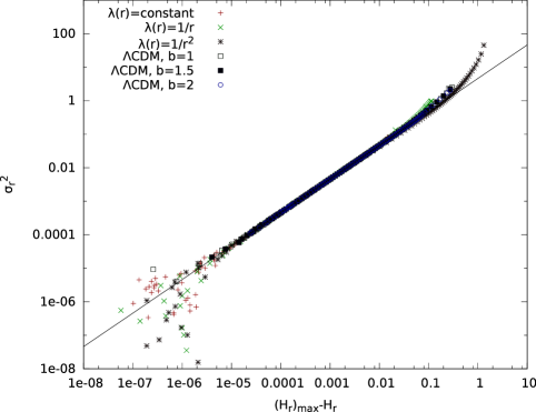
Figure 1: This shows $\sigma_{r}^{2}$ as a function of $(H_{r})_{max}-H_{r}$ for the different distributions considered here. The solid straight line corresponds to the relation $(H_{r})_{max}-H_{r}=\frac{\sigma_{r}^{2}}{4.6}$. Here the factor $\frac{1}{4.6}$ comes from multiplying the factor $\frac{1}{2}$ in Equation 7 with $\frac{1}{\log_{e}10}$.

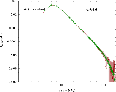
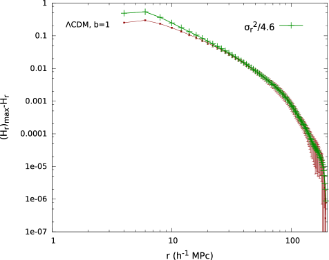
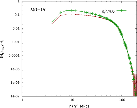
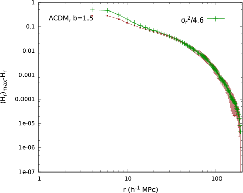
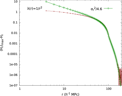
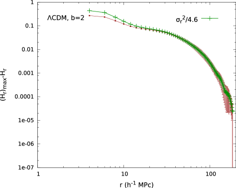
Figure 2: This shows $(H_{r})_{max}-H_{r}$ and $\frac{\sigma_{r}^{2}}{4.6}$ as a function of $r$ for different distributions as indicated in each panel. In each case we have shown only the $1-\sigma$ errorbars for $(H_{r})_{max}-H_{r}$ for clarity.

4 DATA

We use a set of Monte Carlo simulations and N-body simulations to verify the relation between the information entropy and mass variance. We use the same data sets to investigate some possible applications of the information entropy-mass variance relation in cosmology.

4.1 Monte Carlo simulations of homogeneous and inhomogeneous distributions

We generate a set of three dimensional distributions of some homogeneous and inhomogeneous distributions using Monte Carlo simulations. We consider a set of radial density distributions $\rho(r)=K\,\lambda(r)$ where $K$ is a normalization constant. The nature of the distribution is governed by the function $\lambda(r)$ and we consider $3$ different forms for $\lambda(r)$: (i) $\lambda(r)=1$, (ii) $\lambda(r)=\frac{1}{r}$ and (iii) $\lambda(r)=\frac{1}{r^{2}}$. The distribution (i) is a homogeneous and isotropic Poisson point process with same density everywhere whereas the distributions (ii) and (iii) are inhomogeneous Poisson point process. We employ a Monte Carlo dartboard technique to simulate these distributions. The detail of the method can be found in Pandey (2013). Each of the distributions is simulated with $N=10^{5}$ points distributed in a spherical region of radius $R=200{\,h^{-1}\,{\rm Mpc}}$. We generate $10$ such realizations for each of the above distributions.

4.2 N-body simulations

We use data from a set of N-body simulations of the $\Lambda$CDM model carried out using a Particle-Mesh (PM) N-body code (Pandey, 2013). The simulations were run using $256^{3}$ particles on a $512^{3}$ mesh. The simulations cover a comoving volume of $[921.6h^{-1}{\rm Mpc}]^{3}$. We used a $\Lambda$CDM power spectrum with spectral index $n_{s}=0.96$ and normalization $\sigma_{8}=0.812$ (Komatsu et al. 2009) with cosmological parameters $\Omega_{m0}=0.27$, $\Omega_{\Lambda 0}=0.73$ and $h=0.71$. The simulations were run for three different realizations of the initial density fluctuations. We obtain three different realizations of the dark matter distribution at $z=0$ from these simulations. In the current paradigm of structure formation galaxies form at the location of the peaks of the density field. We use a biasing scheme (Cole, Hatton & Weinberg, 1998) where a sharp cutoff is applied to the smoothed density field allowing the galaxies to form only in regions where the overdensity exceeds a certain threshold. Consequently the resulting distributions become biased relative to the dark matter distributions. We determine the linear bias parameter $b$ of each simulated biased sample using the ratio,

$$b=\sqrt{\frac{\xi_{g}(r)}{\xi_{m}(r)}}$$ (10)

where $\xi_{g}(r)$ and $\xi_{m}(r)$ are the two-point correlation functions for the biased distribution and dark matter distribution respectively. We generate biased distributions for three different values of the linear bias $b=1.5$, $b=2$ and $b=2.5$. For each of the biased and unbiased distributions we consider three non-overlapping spherical regions of radius $R=200\,h^{-1}{\rm Mpc}$. We randomly extract $N=10^{5}$ particles from each of these spherical regions. This provides us total nine samples for each bias values.

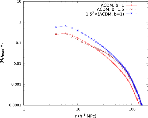
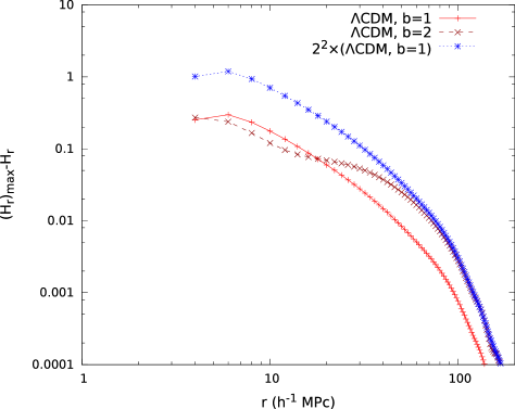
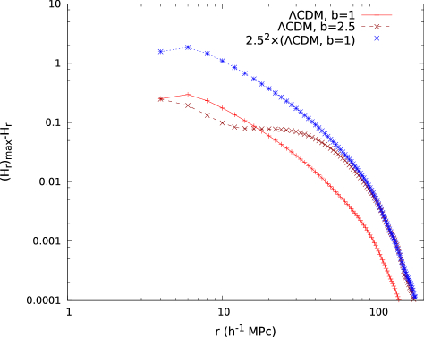
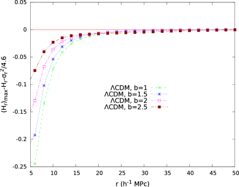
Figure 3: The top left, top right and bottom left panels show that scaling the $(H_{r})_{max}-H_{r}$ values for the unbiased $\Lambda$CDM model with $b^{2}$ exactly reproduce the $(H_{r})_{max}-H_{r}$ values for the different biased $\Lambda$CDM model on large scales. This shows that on large scales the ratio of $(H_{r})_{max}-H_{r}$ values of the galaxy distributions and dark matter distributions from the N-body simulations of the $\Lambda$CDM model can be used to determine the linear bias parameter. The bottom right panel shows the $(H_{r})_{max}-H_{r}-\frac{\sigma_{r}^{2}}{4.6}$ as a function of length scales for the unbiased and biased distributions from the N-body simulations of the $\Lambda$CDM model. The values of $H_{r}$, $(H_{r})_{max}$ and $\sigma_{r}^{2}$ used here are the average values estimated from the $9$ samples for each distributions.

5 Results and Conclusions

We first investigate the relationship between the information entropy and the mass variance for all the distributions described in section 4. We find that in all the distributions though entropy and $\log\sigma_{r}$ show some correlations it is difficult to find any general relation between them. But when we study the relation between the deviation of entropy from its maximum value i.e. $(H_{r})_{max}-H_{r}$ and the mass variance $\sigma_{r}^{2}$ for the same distributions, interestingly we find that they are very tightly correlated (Figure 1). In Figure 1 we find that for a wide range in their values, the relation between these two quantities in all these distributions can be described by a straight line of the form $(H_{r})_{max}-H_{r}=\frac{\sigma_{r}^{2}}{a}$ where $a$ is a constant to be determined. We determine the value of $a$ for each of these distributions by fitting the data with this straight line. We find that the best fit value of $a=4.65\pm 0.03$ is the same for all the distributions when the data is fitted over $(H_{r})_{max}-H_{r}$ in the range $10^{-5}-10^{-1}$. Some deviations from this relation are noticed beyond this range. It is interesting to note that in this regime the relation is exactly described by the relation given in Equation 7. The relation is found to be independent of the nature of the distribution as predicted by the Equation 7. Further we carry out analysis with different sampling rates to find that the relation also does not depend on the number density of the distributions in the appropriate regime as predicted by the same relation.

In Figure 2 we show $(H_{r})_{max}-H_{r}$ and $\frac{\sigma_{r}^{2}}{4.6}$ for different distributions as a function of length scale $r$. In the top left panel we show the results for a homogeneous and isotropic Poisson point process. We find that for this distribution the relation holds very well for nearly the entire length scale range. This is related to the fact that for a homogeneous and isotropic Poisson distribution the only source of fluctuations are shot noise which is only important on small scales. We show the results for the radially inhomogeneous distributions with $\lambda(r)=\frac{1}{r}$ in the middle left panel and $\lambda(r)=\frac{1}{r^{2}}$ in the bottom left panel. Here we find that there are significant deviations from this relation on scales $r\leq 40{\,h^{-1}\,{\rm Mpc}}$. Interestingly the differences decrease with increasing length scales and the results are in excellent agreement with the relation for these distributions beyond the length scales of $r>50{\,h^{-1}\,{\rm Mpc}}$. In the top right, middle right and bottom right panels of Figure 2 we show the results for the $\Lambda$CDM model with different linear bias values as indicated in each panel. We find small departures from the relation in each of these distributions on smaller length scales $r\leq 20{\,h^{-1}\,{\rm Mpc}}$ but the relation holds astonishingly well on length scales of $r>20{\,h^{-1}\,{\rm Mpc}}$. It may be noted in different panels of Figure 2 that the shape of the $(H_{r})_{max}-H_{r}$ curves are quite different from each other which are the characteristics of the respective distributions. But the relation given in Equation 7 holds quite well irrespective of the nature of the distributions. The deviations of the results from Equation 7 in all these distributions originate from the presence of larger fluctuations on those length scales. This retains the non-vanishing higher order terms in Equation 3 giving rise to those differences. But the higher order terms become negligible in the small fluctuation regime where Equation 7 becomes exact. Therefore deviation from the Equation 3 provides the degree of non-linearities present and the length scales where the non-linearities become important in a distribution.

We now investigate if the information entropy-mass variance relation can be used to determine the linear bias and characterize the non-Gaussianities. In the top left panel of Figure 3 we show the $(H_{r})_{max}-H_{r}$ values as a function of length scales for the unbiased ($b=1$) $\Lambda$CDM simulation and its biased counterpart with the bias value $b=1.5$. We see that when the $(H_{r})_{max}-H_{r}$ values for the unbiased distributions are scaled by a factor of $1.5^{2}$, it exactly reproduces the $(H_{r})_{max}-H_{r}$ values for the biased distributions on scales $r>30{\,h^{-1}\,{\rm Mpc}}$. The top right and bottom left panels of Figure 3 similarly show that on scales $r>30{\,h^{-1}\,{\rm Mpc}}$ the $(H_{r})_{max}-H_{r}$ values for the biased distributions with $b=2$ and $b=2.5$ are simply $2^{2}$ and $2.5^{2}$ times the $(H_{r})_{max}-H_{r}$ values of the unbiased distributions on those scales. However it can be clearly seen in all these panels that this simple scaling does not work on smaller scales. The assumption of the scale independent linear bias does not hold on small scales where the non-linearities play an important role. The particles are distributed in diverse environments in an unbiased distribution whereas they are preferentially selected from the density peaks in a biased distribution. In a biased distribution the measuring spheres centered on the particles would encompass regions with similar densities at smaller radii. But the measuring spheres would encompass varying degrees of empty regions beyond the characteristic scales of the density peaks leading to non-uniformity in the measurements with increasing radii. On the other hand, in an unbiased distribution, the measuring spheres would pick up regions of diverse densities at smaller radii reflecting a less uniform behaviour on those scales. The unbiased distribution would be more uniform at larger radii when the measuring spheres would encompass statistically similar number of sites from different environments. This explains why the biased distributions appear to be more uniform on smaller scales and less uniform on larger scales as compared to the unbiased distributions. These characteristic behaviours of the biased distributions give rise to the observed differences from the Equation 9 on smaller scales. Despite these differences it is clear that one can use the ratios of $(H_{r})_{max}-H_{r}$ values of different distributions on large scales to determine their relative bias parameters. The method can be also used to determine the linear bias for galaxies with different physical properties. In future we plan to study the luminosity-bias relation for the galaxies in the SDSS using this method.

In the bottom right panel of Figure 3 we show $(H_{r})_{max}-H_{r}-\frac{\sigma_{r}^{2}}{4.6}$ as a function of length scales for the biased and the unbiased distributions considered here. We find that $(H_{r})_{max}-H_{r}-\frac{\sigma_{r}^{2}}{4.6}<0$ for all the distributions upto a length scales of $\sim 40{\,h^{-1}\,{\rm Mpc}}$ suggesting that all of them are non-Gaussian. We see that it is more negative in the unbiased distributions as compared to the biased distributions. It may be also noted that the measure becomes less negative with increasing bias. This behaviour is possibly related to the fact that a biased distribution becomes more uniform on small scales with increasing bias. However as this measure is a combination of different odd and event moments with alternating signs, it is difficult in general to absolutely compare the degree of non-Gaussianity present in these distributions.

In this work we present a relation between the information entropy and the mass variance and show that on large scales the relation can be used to determine the linear bias from galaxy surveys. The relation may be also employed to constrain the growth rate of density fluctuations and time evolution of linear bias on large scales. On small scales one can use the relation to characterize the non-Gaussianities present in the galaxy distribution. Finally we note that the present analysis suggests that the information entropy can serve as an important tool for the study of large scale structures in the Universe.

6 Acknowledgement

I sincerely thank an anonymous referee for constructive comments and suggestions which helped me to significantly improve the draft. The author would like to acknowledge IUCAA, Pune and CTS, IIT Kharagpur for the use of its facilities for the present work. The author would also like to thank Shreekantha Sil for useful comments and discussions.

References

- Aragón-Calvo et al. (2007) Aragón-Calvo, M. A., van de Weygaert, R., Jones, B. J. T., & van der Hulst, J. M. 2007, ApJ Letters, 655, L5
- Barrow et al. (1985) Barrow, J. D., Bhavsar, S. P., & Sonoda, D. H. 1985, MNRAS, 216, 17
- Bartolo et al. (2004) Bartolo, N., Komatsu, E., Matarrese, S., & Riotto, A. 2004, Physics Reports, 402, 103
- Benoist et al. (1996) Benoist, C., Maurogordato, S., da Costa, L.N., Cappi, A., & Schaeffer, R., 1996, ApJ, 472, 452
- Bharadwaj & Pandey (2004) Bharadwaj, S., & Pandey, B. 2004, ApJ, 615, 1
- Carron & Neyrinck (2012) Carron, J., & Neyrinck, M. C. 2012, ApJ, 750, 28
- Carron (2011) Carron, J. 2011, ApJ, 738, 86
- Cole, Hatton & Weinberg (1998) Cole, S., Hatton, S., Weinberg, D. H., & Frenk, C. S. 1998, MNRAS, 300, 945
- Colombi, Pogosyan & Souradeep (2000) Colombi, S., Pogosyan, D., & Souradeep, T. 2000, Physical Review Letters, 85, 5515
- Einasto et al. (1984) Einasto, J., Klypin, A. A., Saar, E., & Shandarin, S. F. 1984, MNRAS, 206, 529
- Feldman et al. (2001) Feldman, H. A., Frieman, J. A., Fry, J. N., & Scoccimarro, R. 2001, Physical Review Letters, 86, 1434
- Gaztañaga et al. (2005) Gaztañaga, E., Norberg, P., Baugh, C. M., & Croton, D. J. 2005, MNRAS, 364, 620
- Gott, Dickinson, & Melott (1986) Gott, J. R., Dickinson, M., & Melott, A. L. 1986, ApJ, 306, 341
- Hawkins et al. (2003) Hawkins, E., et al.2003, MNRAS,346,78
- Icke & van de Weygaert (1987) Icke, V., & van de Weygaert, R. 1987, A&A, 184, 16
- Komatsu et al. (2009) Komatsu, E., et al. 2009, ApJS, 180, 330
- Mecke et al. (1994) Mecke, K. R., Buchert, T., & Wagner, H. 1994, A&A, 288, 697
- Norberg et al. (2001) Norberg, P., et al. 2001, MNRAS, 328, 64
- Patel, Kapadia & Owen (1976) Patel, J.K., Kapadia, C.H., Owen, D.B. 1976, Handbook of Statistical Distributions, 1976, Marcel Dekker,Inc, New York and Basel
- Pandey & Bharadwaj (2007) Pandey, B., & Bharadwaj, S. 2007, MNRAS, 377, L15
- Pandey (2013) Pandey, B. 2013, MNRAS, 430, 3376
- Pandey & Sarkar (2015) Pandey, B. & Sarkar, S. 2015, MNRAS, 454, 2647
- Pandey & Sarkar (2016) Pandey, B., & Sarkar, S. 2016, MNRAS, 460, 1519
- Pandey (2016) Pandey, B. 2016, MNRAS, 462, 1630
- Peebles (1993) Peebles, P. J. E. 1993, Principles of Physical Cosmology. Princeton, N.J., Princeton University Press, 1993
- Peebles (1980) Peebles, P. J. E. 1980, The large scale structure of the Universe. Princeton, N.J., Princeton University Press, 1980, 435 p.,
- Romano & Siegel (1986) Romano, J.P. & Siegel, A.F. 1986, Counterexamples in Probability And Statistics. ,Boca Raton:Chapman and Hall/CRC, 49 p.,
- Sahni, Sathyaprakash,& Shandarin (1998) Sahni, V., Sathyaprakash, B. S., & Shandarin, S. F. 1998, ApJ Letters, 495, L5
- Sarkar & Bharadwaj (2009) Sarkar, P., & Bharadwaj, S. 2009, MNRAS, 394, L66
- Schmalzing & Buchert (1997) Schmalzing, J., & Buchert, T. 1997, ApJ Letters, 482, L1
- Shandarin & Zeldovich (1983) Shandarin, S. F. & Zeldovich, I. B. 1983, Comments on Astrophysics, 10, 33
- Shannon (1948) Shannon, C. E. 1948, Bell System Technical Journal, 27, 379-423, 623-656
- Stoica et al. (2005) Stoica, R. S., Martínez, V. J., Mateu, J., & Saar, E. 2005, A&A, 434, 423
- Sousbie et al. (2008) Sousbie, T., Pichon, C., Colombi, S., Novikov, D., & Pogosyan, D. 2008, MNRAS, 383, 1655
- Tegmark et al. (2004) Tegmark, M., et al. 2004, ApJ, 606, 702
- van de Weygaert & Icke (1989) van de Weygaert, R., & Icke, V. 1989, A&A, 213, 1
- Verde et al. (2002) Verde, L., Heavens, A. F., Percival, W. J., et al. 2002, MNRAS, 335, 432
- White (1979) White, S. D. M. 1979, MNRAS, 186, 145
- York et al. (2000) York, D. G., et al. 2000, AJ, 120, 1579
- Zehavi et al. (2011) Zehavi, I., Zheng, Z., Weinberg, D. H., et al. 2011, ApJ, 736, 59