Practical stabilization of perturbed integrator chains with unknown bounds

Abstract

In this paper, we present Lyapunov-based adaptive controllers for the practical (or real) stabilization of a perturbed chain of integrators with bounded uncertainties. We refer to such controllers as Adaptive Higher Order Sliding Mode (AHOSM) controllers since they are designed for nonlinear SISO systems with bounded uncertainties such that the uncertainty bounds are unknown. Our main result states that, given any neighborhood $\displaystyle\cal{N}$ of the origin, we determine a controller insuring, for every uncertainty bounds, that every trajectory of the corresponding closed loop system enters $\displaystyle\cal{N}$ and eventually remains there. The effectiveness of these controllers is illustrated through simulations.

I Introduction

Parametric uncertainty in nonlinear dynamic physical systems arises from varying operating conditions and external perturbations that affect the physical characteristics of such systems. The variation limits or the bounds of this uncertainty might be known or unknown. This needs to be considered during control design so that the controller counteracts the effect of variations and guarantees performance under different operating conditions. Sliding mode control (SMC) [1, 2] is a well-known method for control of nonlinear systems, renowned for its insensitivity to parametric uncertainty and external disturbance. This technique is based on applying discontinuous control on a system which ensures convergence of the output function (sliding variable) in finite time to a manifold of the state-space, called the sliding manifold [3]. In practice, SMC suffers from chattering; the phenomenon of finite-frequency, finite-amplitude oscillations in the output which appear because the high-frequency switching excites unmodeled dynamics of the closed loop system [4]. Higher Order Sliding Mode Control (HOSMC) is an effective method for chattering attenuation [5]. In this method the discontinuous control is applied on a higher time derivative of the sliding variable, such that not only the sliding variable converges to the origin, but also its higher time derivatives. As the discontinuous control does not act upon the system input directly, chattering is automatically reduced.

Many HOSMC algorithms exist in contemporary literature for control of uncertain nonlinear systems, where the bounds on uncertainty are known. These are robust because they preserve the insensitivity of classical sliding mode, and maintain the performance characteristics of the closed loop system as long as it remains inside the defined uncertainty bounds. Levant for example, has presented a method of designing arbitrary order sliding mode controllers for Single Input Single Output (SISO) systems in [6]. In his recent works [7, 8], homogeneity approach has been used to demonstrate finite time stabilization of the proposed method. Laghrouche et al. [9] have proposed a two part integral sliding mode based control to deal with the finite time stabilization problem and uncertainty rejection problem separately. Dinuzzo et al. have proposed another method in [10], where the problem of HOSM has been treated as Robust Fuller’s problem. Defoort et al. [11] have developed a robust Multi Input Multi Output (MIMO) HOSM controller, using a constructive algorithm with geometric homogeneity based finite time stabilization of a chain of integrators. Harmouche et al. have also presented their homogeneous controller in [12] based on the work of Hong [13].

The case where the bounds on uncertainty exist, but are unknown, is an interesting problem in the field of arbitrary HOSMC. In this problem, a good control strategy is expected to have two essential properties: (a) no use of the uncertainty bounds in the stabilizing controller design; (b) avoidance of gain overestimation [14]. In recent years, adaptive sliding mode controllers have attracted the interest of many researchers for this case[15, 16, 17, 18]. Adaptive gains have been used with success in the past for chattering suppression. For example, Bartolini et al. [19] have extended Utkin’s concept of equivalent control for second order sliding mode control gain adaptation, to suppress residual oscillations due to digital controllers with time delay. Similarly, an equivalent control based adaptive controller is described in [20], in which the equivalent control estimation is improved, using double low pass filters. A concise survey of these methods can be found in [21]. Huang et al. [22] were the first to use dynamic gain adaptation in SMC for the problem of unknown uncertainty bounds. They presented an adaptation law for first order SMC, which depends directly upon the sliding variable; the control gains increase until sliding mode is achieved, and afterwards the gains become constant. This method works without a-priori knowledge of uncertainty bounds, however it does not solve the gain overestimation problem as the gains stabilize at unnecessarily large values. Plestan et al. [14, 23] have overcome this problem by slowly decreasing the gains once sliding mode is achieved. This method establishes real sliding mode (convergence to a neighborhood of the sliding surface). However it does not guarantee that the states would remain inside the neighborhood after convergence; the state actually overshoots in a region around the neighborhood depending on the uncertainties bounds, which is therefore not known. In the field of HOSMC, Shtessel et al. [24] have presented a Second Order adaptive gain SMC for non-overestimation of the control gains, based on a supertwisting algorithm. An adaptive version of the twisting algorithm is proposed in [25], and applied for pneumatic actuator control. The state overshoots in the cases of [24] and [25] as well. However, unlike [14], the magnitude is unknown. A Lyapunov-based variable gains super twisting algorithm has also been presented in [26]. Glumineau et al. [27] have presented a different approach, based on impulsive sliding mode adaptive control of a double integrator system. The gain of the impulsive control is adapted to minimize the convergence time of the double integrator dynamics. In [28] and [29] continuous AHOSM control algorithms are studied. They are based on reconstruction of equivalent control. All these works insure sliding set convergence to a bounded zone whose size and convergence time depend upon the upper bounds of the perturbations or their derivatives. In particular, if these upper bounds are not a priori known, one cannot prescribe in advance the size of the convergence zone.

It can be noted that all research works avoiding gain overestimation, discussed so far, have yielded real sliding mode. In fact, real sliding mode is the only possibility when the uncertainty bounds are unknown, as the gain dynamics cannot respond immediately to sudden changes in system parameters.

In this paper, we present Lyapunov-based adaptive controllers for the finite time stabilization of a perturbed chain of integrators with bounded uncertainties. Through a minor extension of the definition (as explained in the next section), we refer to such controllers as Adaptive Higher Order Sliding Mode controllers (AHOSM controllers or AHOSMC). The proposed adaptive controller guarantees finite time convergence to an adjustable arbitrary neighborhood of origin whose size does not depends upon the upper bounds of the perturbations or their derivatives, i.e., it establishes real HOSM. The advantage of this adaptive controller design, compared to other controllers mentioned before, is that this controller can be extended to arbitrary order and the adaptation rates are fast in both directions. In addition, the state is confined inside the neighborhood after convergence and cannot escape. As a result, there is no state overshoot and no gain overestimation in this controller; and the neighborhood of convergence can be chosen as small as possible independently of the upper bounds of the perturbations or their derivatives.

The paper is organized as follows: problem formulation and adaptive controllers are presented in Section 2, simulation results are shown in Section 3. Some concluding remarks are given in Section 4.

II Higher Order Sliding Mode Controllers

If $\displaystyle r$ is a positive integer, the perturbed chain of integrators of length $\displaystyle r$ corresponds to the (uncertain) control system given by

$$\begin{array}[]{lcl}\dot{z}_{r}=\varphi(t)+\gamma(t)u,\end{array}$$ (1)

where $\displaystyle z=[z_{1}\ z_{2}\ ...z_{r}]^{T}\in\mathbb{R}^{r}$, $\displaystyle u\in\mathbb{R}$ and the functions $\displaystyle\varphi$ and $\displaystyle\gamma$ are any measurable functions defined almost everywhere (a.e. for short) on $\displaystyle\mathbb{R}_{+}$ and bounded by positive constants $\displaystyle\bar{\varphi}$, $\displaystyle\gamma_{m}$ and $\displaystyle\gamma_{M}$, such that, for a.e. $\displaystyle t\geq 0$,

$$\begin{array}[]{lcl}\left|\varphi(t)\right|\leq\bar{\varphi},\quad 0<\gamma_{m}\leq\gamma(t)\leq\gamma_{M}.\end{array}$$ (2)

One can equivalently define a perturbed chain of integrators of length $\displaystyle r$ as the differential inclusion $\displaystyle\dot{z}_{r}\in I_{\bar{\varphi}}+uI_{\gamma}$ where $\displaystyle I_{\bar{\varphi}}=\left[-\bar{\varphi},\bar{\varphi}\right]$ and $\displaystyle I_{\gamma}=\left[\gamma_{m},\gamma_{M}\right]$.

The usual objective regarding System (1) consists of stabilizing it with respect to the origin in finite time, i.e., determining feedback laws $\displaystyle u=U(z)$ so that the trajectories of the corresponding closed-loop system converge to the origin in finite time. Note that, in general, the controllers $\displaystyle U(\cdot)$ are discontinuous and then, solutions of (1) need to be understood here in Filippov’s sense [30], i.e., the right-hand vector set is enlarged at the discontinuity points of the differential inclusion to the convex hull of the set of velocity vectors obtained by approaching $\displaystyle z$ from all directions in $\displaystyle\mathbb{R}^{r}$, while avoiding zero-measure sets. Several solutions for this problem exist [31, 32, 8, 9, 33] under the hypothesis that the bounds $\displaystyle\gamma_{m},\gamma_{M}$ and $\displaystyle\bar{\varphi}$ are known.

In case the bounds $\displaystyle\gamma_{m},\gamma_{M}$ and $\displaystyle\bar{\varphi}$ are unknown (one only assumes their existence) then it is obvious to see that finite time stabilization is not possible by a mere state feedback and therefore, one possible alternate objective consists in achieving practical stabilization. This is the goal of this paper to establish such a result for System (1) and we provide next a precise definition of practical stabilization.

Definition 1.

We say that $\displaystyle\dot{z}=f(z,u)$ is practically stabilizable, if for every $\displaystyle\varepsilon>0$, there exists a controller $\displaystyle u=U_{\varepsilon}(\cdot,t)$ such that every trajectory of the closed-loop system $\displaystyle\dot{z}=f(z,U_{\varepsilon}(\cdot,t))$ enters the open ball of radius $\displaystyle\varepsilon$ centered at the origin and eventually remains there.

The main result of that paper consists of designing controllers which practically stabilize System (1) independently of the positive bounds $\displaystyle\bar{\varphi}$, $\displaystyle\gamma_{m}$ and $\displaystyle\gamma_{M}$, i.e., for every $\displaystyle\varepsilon>0$, the controllers $\displaystyle u=U_{\varepsilon}(\cdot,t)$ which practically stabilize System (1) does not depend on the bounds $\displaystyle\bar{\varphi}$, $\displaystyle\gamma_{m}$ and $\displaystyle\gamma_{M}$.

We next recall the following definition needed in the sequel.

Definition 2.

(Homogeneity. cf. [32].) If $\displaystyle r,m$ are positive integers, a function $\displaystyle f:\mathbb{R}^{r}\rightarrow\mathbb{R}^{m}$ (or a differential inclusion $\displaystyle F:\mathbb{R}^{r}\rightrightarrows\mathbb{R}^{m}$ respectively) is said to be homogeneous of degree $\displaystyle q\in\mathbb{R}$ with respect to the family of dilations $\displaystyle\delta_{\varepsilon}(z)$, $\displaystyle\varepsilon>0$, defined by

$$\delta_{\varepsilon}(z)=(z_{1},\cdots,z_{r})\mapsto(\varepsilon^{p_{1}}z_{1},\cdots,\varepsilon^{p_{r}}z_{r}),$$

where $\displaystyle p_{1}\cdots,p_{r}$ are positive real numbers (the weights), if for every positive $\displaystyle\varepsilon$ and $\displaystyle z\in\mathbb{R}^{r}$, one has $\displaystyle f(\delta_{\varepsilon}(z))=\varepsilon^{q}f(z)$ $\displaystyle\big{(}F(\delta_{\varepsilon}(z))=\varepsilon^{q}\delta_{\varepsilon}(F(z))\ respectively\big{)}$.

The following notations will be used throughout the paper. We define the function $\displaystyle sgn$ as the multivalued function defined on $\displaystyle\mathbb{R}$ by $\displaystyle sgn(x)=\frac{x}{|x|}$ for $\displaystyle x\neq 0$ and $\displaystyle sgn(0)=[-1,1]$. Similarly, for every $\displaystyle a\geq 0$ and $\displaystyle x\in\mathbb{R}$, we use $\displaystyle\left\lfloor x\right\rceil^{a}$ to denote $\displaystyle\left|x\right|^{a}\text{sgn}(x)$. Note that $\displaystyle\left\lfloor\cdot\right\rceil^{a}$ is a continuous function for $\displaystyle a>0$ and of class $\displaystyle C^{1}$ with derivative equal to $\displaystyle a\left|\cdot\right|^{a-1}$ for $\displaystyle a\geq 1$. Moreover, for every positive integer $\displaystyle r$, we use $\displaystyle J_{r}$ to denote the $\displaystyle r$-th Jordan block, i.e., the $\displaystyle r\times r$ matrix whose $\displaystyle(i,j)$-coefficient is equal to $\displaystyle 1$ if $\displaystyle i=j-1$ and zero otherwise.

II-A Adaptive Higher Order Sliding Mode Controller

We first define the system under study and provide parameters used later on.

Definition 3.

Let $\displaystyle r$ be a positive integer. The $\displaystyle r$-th order chain of integrator $\displaystyle(CI)_{r}$ is the single-input control system given by

$$\begin{array}[]{lcl}(CI)_{r}\ \ \ \dot{z}=J_{r}z+ue_{r},\end{array}$$ (3)

with $\displaystyle z=(z_{1},\cdots,z_{r})^{T}\in\mathbb{R}^{r}$ and $\displaystyle u\in\mathbb{R}$. For $\displaystyle\kappa<0$ and $\displaystyle p>0$ with $\displaystyle p+(r+1)\kappa\in[0,1)$, set $\displaystyle p_{i}:=p+(i-1)\kappa,\ 1\leq i\leq r+2$. For $\displaystyle\varepsilon>0$, let $\displaystyle\delta_{\varepsilon}:\mathbb{R}^{r}\rightarrow\mathbb{R}^{r}$ be the family of dilations associated with $\displaystyle\left(p_{1},\cdots,p_{r}\right)$.

In the spirit of [33, 34], we put forwards geometric conditions on certain stabilizing feedbacks $\displaystyle u_{0}(\cdot)$ for $\displaystyle(CI)_{r}$ and corresponding Lyapunov functions $\displaystyle V_{1}$. These conditions will be instrumental for the latter developments.

Our construction of the feedback for practical stabilization relies on the following result.

Theorem 1.

Let $\displaystyle r$ be a positive integer. There exists a feedback law $\displaystyle u_{0}:\mathbb{R}^{r}\rightarrow\mathbb{R}$ homogeneous with respect to $\displaystyle(\delta_{\varepsilon})_{\varepsilon>0}$ such that the closed-loop system $\displaystyle\dot{z}=J_{r}z+u_{0}(z)e_{r}$ is finite time globally asymptotically stable with respect to the origin and the following conditions hold true:

$\displaystyle(i)$

the function $\displaystyle z\mapsto J_{r}z+u_{0}(z)e_{r}$ is homogeneous of degree $\displaystyle\kappa$ with respect to $\displaystyle(\delta_{\varepsilon})_{\varepsilon>0}$ and there exists a continuous positive definite function $\displaystyle V_{1}:\mathbb{R}^{r}\rightarrow\mathbb{R}_{+}$, $\displaystyle C^{1}$ except at the origin, homogeneous with respect to $\displaystyle(\delta_{\varepsilon})_{\varepsilon>0}$ such that there exists $\displaystyle c>0$ and $\displaystyle\alpha\in(0,1)$ for which the time derivative of $\displaystyle V_{1}$ along non trivial trajectories of $\displaystyle\dot{z}=J_{r}z+u_{0}(z)e_{r}$ verifies

$$\begin{array}[]{lcl}\dot{V}_{1}\leq-cV_{1}^{\alpha};\end{array}$$ (4)

$\displaystyle(ii)$

the function $\displaystyle z\mapsto u_{0}(z)\partial_{r}V_{1}(z)$ is non positive over $\displaystyle\mathbb{R}^{r}$ and, for every non zero $\displaystyle z\in\mathbb{R}^{r}$ verifying $\displaystyle u_{0}(z)=0$, one has $\displaystyle\partial_{r}V_{1}(z)=0$. As a consequence function $\displaystyle z\mapsto sgn(u_{0}(z))\partial_{r}V_{1}(z)$ is well-defined over $\displaystyle\mathbb{R}^{r}$ and non positive.

Remark 1.

Item $\displaystyle(i)$ of the above theorem is classical, see for instance [13, 35, 36, 37]. Item $\displaystyle(ii)$ considers a geometric condition on controllers verifying Item $\displaystyle(i)$, which was introduced in [34] and used in [33, 38]. This geometric condition is indeed satisfied, for instance by Hong’s controller, see [38] for other examples.

Regarding our problem, we consider, for every $\displaystyle\varepsilon>0$ the following controller:

$$\begin{array}[]{lcl}u_{\varepsilon}(z,t)=g(|u_{0}(z)|)u_{0}(z)+k\,\hbox{sgn}\big{(}u_{0}(z))\hat{\varphi}_{\varepsilon}(t,V_{1}(z)\big{)},\end{array}$$ (5)

where $\displaystyle u_{0}$ and $\displaystyle V_{1}$ are provided by Theorem 1, $\displaystyle g:\mathbb{R}_{+}\rightarrow\mathbb{R}_{+}^{*}$ is an increasing $\displaystyle C^{1}$ function with $\displaystyle\lim_{x\rightarrow+\infty}g(x)=+\infty$ and the adaptive function $\displaystyle\hat{\varphi}_{\varepsilon}$ is defined as

$$\begin{array}[]{lcl}\hat{\varphi}_{\varepsilon}(t,x)&=&\left\{\begin{array}[]{ccc}\min\big{(}t,F_{\varepsilon}(x)\big{)},&\text{ if }0\leq x<\varepsilon,&\\ t,&\text{ if }x\geq\varepsilon,&\end{array}\right.\end{array}$$ (6)

with $\displaystyle F_{\varepsilon}(x)=\frac{\varepsilon}{\varepsilon-x}$ for $\displaystyle x\in[0,\varepsilon)$. Here the positive function $\displaystyle g$ and the positive constant $\displaystyle k$ are gain parameters whereas $\displaystyle\varepsilon>0$ will be used to define the arbitrarily small neighborhood where trajectories of (1) with feedback control law (5) will eventually end up.

The following theorem provides the main result for the adaptive controller $\displaystyle u_{\varepsilon}$.

Theorem 2.

Let $\displaystyle r$ be a positive integer and System (1) be the perturbed $\displaystyle r$-chain of integrators with unknown bounds $\displaystyle\gamma_{m},\gamma_{M}$ and $\displaystyle\bar{\varphi}$. Let $\displaystyle\varepsilon>0$ and $\displaystyle u_{0},V_{1}:\mathbb{R}^{r}\rightarrow\mathbb{R}_{+}$ be the feedback law and the continuous positive definite function defined respectively in Theorem 1. Then, for every trajectory $\displaystyle z(\cdot)$ of the closed-loop system (1) under the feedback control law (5), one has

$$\begin{array}[]{lcl}\limsup_{t\rightarrow\infty}V_{1}(z(t))\leq\max\big{(}0,\overline{V}_{1}\big{)},\end{array}$$ (7)

where $\displaystyle\overline{V}_{1}:=\varepsilon(1-\frac{1}{\bar{\Phi}})$, with $\displaystyle\bar{\Phi}:=\frac{1}{k\gamma_{m}}\left(\bar{\varphi}-h_{m}\right)$, where $\displaystyle h_{m}=\min\big{(}0,\min_{x\geq 0}(\gamma_{m}g(x)-1)x\big{)}$.

II-B Proof of Theorem 2

We refer to $\displaystyle(S)$ as the closed-loop system defined by (1) and (5). The first issue we address is the existence of trajectories of $\displaystyle(S)$ starting at any initial condition $\displaystyle z_{0}\in\mathbb{R}^{r}$. Such an existence follows from the fact that the application $\displaystyle\mathbb{R}_{+}\times\mathbb{R}^{r}\rightarrow\mathbb{R}$, $\displaystyle(t,z)\mapsto\hat{\varphi}_{\varepsilon}(t,V_{1}(z))$ is continuous.

We next show that every trajectory of $\displaystyle(S)$ is defined for all positive times. For that purpose, consider a non trivial trajectory $\displaystyle z(\cdot)$ and let $\displaystyle I_{z(\cdot)}$ be its (non trivial) domain of definition. We obtain the following inequality for the time derivative of $\displaystyle V_{1}(z(\cdot))$ on $\displaystyle I_{z(\cdot)}$ by using Items $\displaystyle(i)$ and $\displaystyle(ii)$ of Theorem 1. For a.e. $\displaystyle t\in I_{z(\cdot)}$, one gets

$$\begin{array}[]{lcl}\dot{V}_{1}&=&\frac{\partial V_{1}}{\partial z_{1}}z_{2}+...+\frac{\partial V_{1}}{\partial z_{r}}\left(\gamma\left[g(|u_{0}|)u_{0}+k\,\text{sgn}(u_{0})\hat{\varphi}_{\varepsilon}\right]+\varphi\right),\\ &\leq&-cV_{1}^{\alpha}\!-\!\!\left|\frac{\partial V_{1}}{\partial z_{r}}\right|\!\!\Big{(}\!(\gamma_{m}g(|u_{0}|)-1)|u_{0}|\!+\!k\gamma_{m}\hat{\varphi}_{\varepsilon}\!-\!\bar{\varphi}\Big{)},\\ &\leq&-cV_{1}^{\alpha}-k\gamma_{m}\left|\frac{\partial V_{1}}{\partial z_{r}}\right|\left(\hat{\varphi}_{\varepsilon}-\bar{\Phi}\right).\end{array}$$ (8)

We thus have the differential inequality a.e. for $\displaystyle t\in I_{z(\cdot)}$

$$\begin{array}[]{lcl}\dot{V}_{1}\leq-cV_{1}^{\alpha}+C_{1}V_{1}^{p_{r+2}},\end{array}$$ (9)

where $\displaystyle C_{1}$ is a positive constant independent of the trajectory $\displaystyle z(\cdot)$. Since $\displaystyle p_{r+2}\in[0,1)$, it is therefore immediate to deduce that there is no blow-up in finite time and thus $\displaystyle I_{z(\cdot)}=\mathbb{R}_{+}$.

We now prove that Eq. (7) holds true for any trajectory $\displaystyle z(\cdot)$ of $\displaystyle(S)$. Assume first that $\displaystyle 1\geq\bar{\Phi}$. Then, for $\displaystyle t>\bar{\Phi}$, one has that $\displaystyle\hat{\varphi}_{\varepsilon}(t)\geq\bar{\Phi}$ since $\displaystyle F_{\varepsilon}$ takes values larger than $\displaystyle 1$. It implies that $\displaystyle\dot{V}_{1}\leq-cV_{1}^{\alpha}$ and thus one gets convergence to zero in finite time. Assume next that $\displaystyle 1<\bar{\Phi}$. Set $\displaystyle\overline{V}_{1}:=\varepsilon(1-\frac{1}{\bar{\Phi}})$ and notice that $\displaystyle F_{\varepsilon}(\overline{V}_{1})=\bar{\Phi}$. In that case, for $\displaystyle t>\bar{\Phi}$, Eq. (8) can be written

$$\begin{array}[]{lcl}\dot{V}_{1}\leq-cV_{1}^{\alpha}-k\gamma_{m}\left|\frac{\partial V_{1}}{\partial z_{r}}\right|\min(0,F_{\varepsilon}(V_{1}(z))-F_{\varepsilon}(\overline{V}_{1})).\end{array}$$ (10)

Taking into account the fact that $\displaystyle F_{\varepsilon}$ is an increasing function on $\displaystyle[0,\varepsilon)$, one deduces that there exists at most one time $\displaystyle\bar{t}>1$ such that $\displaystyle V_{1}(z(\bar{t}))=\overline{V}_{1}$ (since $\displaystyle\dot{V}_{1}(\bar{t})\leq-c\overline{V_{1}}^{\alpha}<0$) and if it exists, then $\displaystyle V_{1}(z(t))<\overline{V_{1}}$ for $\displaystyle t>\bar{t}$. If such a time $\displaystyle\bar{t}$ does not exists, then one has necessarily $\displaystyle V_{1}(z(t))<\overline{V_{1}}$ for $\displaystyle t>\bar{\Phi}$ since the other alternative would yield convergence in finite time and thus a contradiction.

Remark 2.

In case the controller $\displaystyle u_{0}$ is bounded, one can remove the assumption that $\displaystyle\lim_{x\rightarrow+\infty}g(x)=+\infty$.

II-C Asymptotic bounds for the controller $\displaystyle u$ and the convergence time to the neighborhood $\displaystyle{\cal{V}}_{\varepsilon}$

One deduces from Theorem 2 the following two results. The first one is immediate and provides an asymptotic upper bound for the controller $\displaystyle u$.

Lemma 1.

For $\displaystyle\varepsilon>0$, the controller $\displaystyle u_{\varepsilon}$ defined in (5) verifies the following asymptotic upper bound, which is uniform with respect to trajectories of the closed-loop system $\displaystyle(S)$: if $\displaystyle 1\geq\bar{\Phi}$, then $\displaystyle\lim_{t\rightarrow\infty}{|u_{\varepsilon}|}=1$ and if $\displaystyle 1<\bar{\Phi}$, then

$$\begin{array}[]{lcl}\limsup_{t\rightarrow\infty}{|u_{\varepsilon}|}\leq U_{0}(\overline{V}_{1})g(U_{0}(\overline{V}_{1}))+k\bar{\Phi},\end{array}$$ (11)

where $\displaystyle U_{0}(\xi):=\max_{\{z\,|\,V_{1}(z)\leq\xi\}}|u_{0}(z)|$ for $\displaystyle\xi\geq 0$.

For $\displaystyle\varepsilon>0$, define the open neighborhood $\displaystyle{\cal{V}}_{\varepsilon}$ of the origin as the set of points $\displaystyle z\in\mathbb{R}^{r}$ such that $\displaystyle V_{1}(z)<\varepsilon$. Our second result provides an asymptotic upper bound for the time needed by any trajectory of the closed-loop system $\displaystyle(S)$ to eventually enter $\displaystyle{\cal{V}}_{\varepsilon}$ and remain inside.

Proposition 1.

For $\displaystyle z_{0}\in\mathbb{R}^{r}$, the convergence time $\displaystyle T_{z_{0}}$ needed to reach the open neighborhood $\displaystyle{\cal{V}}_{\varepsilon}$ of the origin and stay inside verifies the following bound:

$$\begin{array}[]{lcl}T_{z_{0}}\leq\bar{\Phi}+\frac{\Big{(}V_{1}^{1-p_{r+2}}(z_{0})+(1-p_{r+2})C_{1}\bar{\Phi}\Big{)}^{\frac{1-\alpha}{1-p_{r+2}}}}{c(1-\alpha)},\end{array}$$ (12)

where the constants $\displaystyle c,\alpha$ are provided by Theorem 1 and the constants $\displaystyle\beta,C_{1}$ are defined in Eq. (9).

Proof.

For $\displaystyle t\leq\bar{\Phi}$, one deduces from Eq. (9) the upper bound

$$V_{1}(z(\Phi))\leq\Big{(}V_{1}^{1-p_{r+2}}(z_{0})+(1-p_{r+2})C_{1}\bar{\Phi}\Big{)}^{\frac{1}{1-p_{r+2}}}.$$

For $\displaystyle t\geq\bar{\Phi}$, $\displaystyle V_{1}$ verifies either Eq. (4) or Eq. (10), which reduces to Eq. (4) if $\displaystyle z(t)\notin{\cal{V}}_{\varepsilon}$. It is then clear that the right-hand side of Eq. (12) is an upper bound for $\displaystyle T_{z_{0}}$. ∎

III Simulation Results

The performances of the proposed control law are studied next through simulation. In this section we will perform simulations for uncertain systems of order one and three.

III-A Simulation for first order system

Consider the first order system

$$\displaystyle\dot{z}_{1}=\varphi+\gamma u,$$

where $\displaystyle\gamma$ and $\displaystyle\varphi$ are discontinuous bounded uncertainties defined as

$$\begin{array}[]{lcl}\varphi=5\text{sgn}(cos(t))-10\sin(2t),\gamma=3+2\text{sgn}(\sin(3t)).\end{array}$$ (13)

One can see that

$$\displaystyle 0<1\leq\gamma\leq 5,\ |\varphi|\leq 15.$$

The candidate $\displaystyle u_{0}$ and its related Lyapunov function are given next as:

$$\displaystyle u_{0}=-\text{sgn}(z_{1}),\quad V_{1}=|z_{1}|.$$

The control objective consists to force $\displaystyle z_{1}$ to the neighborhood of zero defined by $\displaystyle V_{1}:=|z_{1}|\leq\epsilon:=0.1$. Based on the given $\displaystyle u_{0}$ with simple computation, the controller $\displaystyle u$ can be defined as

$$\begin{array}[]{lcl}u=-\left(1+\varphi_{\varepsilon}(t)\right)\text{sgn}(z_{1}).\end{array}$$ (14)

The performance of the proposed controller with respect to the uncertainties is presented in Figure 1. On can see in Figure 1(b), the convergence of the state $\displaystyle z_{1}$ the predefined neighborhood of zero. The control objective is satisfied without overestimation of the controller as seen in Figure 1(a).

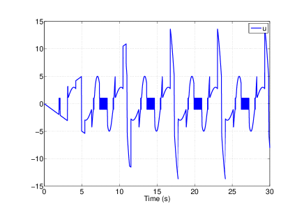
(a) Control law $\displaystyle u$

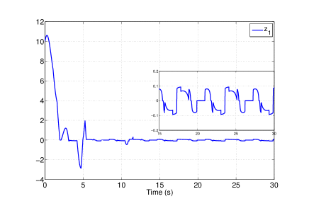
(b) State $\displaystyle z_{1}$

Figure 1: Simulation for order 1

III-B Simulation for third order system

For arbitrary order, we can refer to Hong’s controller [39] as candidate for the controller $\displaystyle u_{0}$ defined as follows. Let $\displaystyle\kappa<0$ and $\displaystyle l_{1},\cdots,l_{r}$ positive real numbers. For $\displaystyle z=(z_{1},\cdots,z_{r})$, we define for $\displaystyle i=0,...,r-1$:

$$\begin{array}[]{lcl}p_{i}=1+(i-1)\kappa,\\ v_{0}=0,\,v_{i+1}=-l_{i+1}\lfloor\lfloor z_{i+1}\rceil^{\beta_{i}}-\lfloor v_{i}\rceil^{\beta_{i}}\rceil^{(\alpha_{i+1}/(\beta_{i})},\\ u_{0}=v_{r},\end{array}$$ (15)

where $\displaystyle\alpha_{i}=\frac{p_{i+1}}{p_{i}}$.
The Lyapunov Function candidate $\displaystyle V_{1}$ is defined in the following form:

$$\begin{array}[]{lcl}{V_{1}}=\sum\limits_{j=1}^{r}\int\limits_{{v_{j-1}}}^{{z_{j}}}{{{\left\lfloor s\right\rceil}^{{\beta_{j-1}}}}-{{\left\lfloor{{v_{j-1}}}\right\rceil}^{{\beta_{j-1}}}}ds}.\end{array}$$ (16)

In this section, we consider the following third order system

$$\displaystyle\dot{z}_{1} \displaystyle= \displaystyle z_{2},$$

$$\displaystyle\dot{z}_{2} \displaystyle= \displaystyle z_{3},$$

$$\displaystyle\dot{z}_{3} \displaystyle= \displaystyle\varphi+\gamma u,$$

with the same uncertainty as given in previous simulations. In this simulation, the control parameters of $\displaystyle u_{0}$ have been tuned to the following values

$$\begin{array}[]{lcl}l_{1}=1,\ l_{2}=2,\ l_{3}=5,\ \kappa=-1/4.\end{array}$$ (17)

The function $\displaystyle g(u_{0})$ has been taken as

$$\begin{array}[]{lcl}g(u_{0})=1+\log(1+|u_{0}|).\end{array}$$ (18)

The control objective consists to force the states $\displaystyle z_{1},\ z_{2},\ z_{3}$ to a neighborhood of zero defined by $\displaystyle\left\{z=(z_{1},z_{2},z_{3}):V_{1}(z_{1},z_{2},z_{3})\leq 0.01\right\}$. In Figure 2(b), one can see the practical convergence of $\displaystyle z_{1}$, $\displaystyle z_{2}$ and $\displaystyle z_{3}$. The control objective is achieved as seen in Figure 2(d), where $\displaystyle LLV1:=\log(1+V_{1})$. The controller and the adaptive gain are presented in Figure 2(a) and Figure 2(c) respectively.

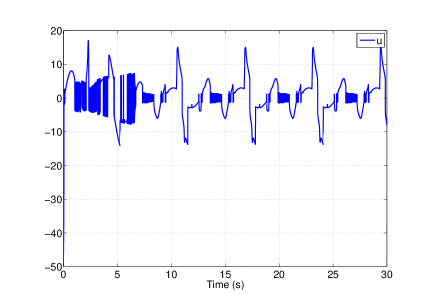
(a) Control law $\displaystyle u$

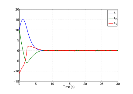
(b) State $\displaystyle z_{1}$

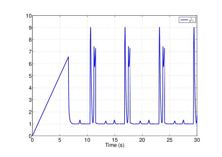
(c) Adaptive gain $\displaystyle\hat{\varphi}_{\varepsilon}$

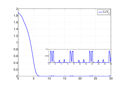
(d) Lyapunov Function

Figure 2: Simulation for order 3

IV Conclusions

This paper has proposed a new Lyapunov-based adaptive scheme for higher-order sliding mode controller with bounded unknown uncertainties. The proposed adaptive controller guarantees finite time convergence to an adjustable arbitrary neighborhood of origin. The advantage of this adaptive controller, compared to others, is that this controller can be extended to any arbitrary order. In addition, the state is confined inside the neighborhood after convergence and cannot escape. As a result, there is no state overshoot and no gain overestimation in this controller; and the neighborhood of convergence can be chosen as small as possible.

References

- [1] V. I. Utkin. Sliding Mode Control and Optimization. Springer Verlag, Berlin, 1992.
- [2] J.J. Slotine. Sliding mode controller design for non-linear systems. International Journal of Control, 40:421 – 434, 1984.
- [3] K.D. Young, V.I. Utkin, and U. Ozguner. A control engineer’s guide to sliding mode control. IEEE Transactions on Control System Technology, 7(3):328–342, 1999.
- [4] V. I. Utkin, J. Guldner, and J. Shi. Sliding mode in control in electromechanical systems. London: Taylor and Francis, 1999.
- [5] S.V. Emel’yanov, S.K. Korovin, and A. Levant. High-order sliding modes in control systems. Computational Mathematics and Modeling, 7(3):294–318, 1996.
- [6] A. Levant. Universal Single-Inupte Single-Output (SISO) Sliding-Mode Controllers With Finite-Time Convergence. IEEE Transactions on Automatic Control, 46(9):1447 – 1451, 2001.
- [7] A. Levant. Higher-order sliding modes, differentiation and output-feedback control. International Journal of Control, 76(9/10):924 – 941, 2003.
- [8] A. Levant. Homogeneity approach to high-order sliding mode design. Automatica, 41(5):823 – 830, 2005.
- [9] S. Laghrouche, F. Plestan, and A. Glumineau. Higher order sliding mode control based on integral sliding mode. Automatica, 43:531–537, March 2007.
- [10] F. Dinuzzo and A. Ferrara. Higher Order Sliding Mode Controllers with Optimal Reaching. IEEE Transactions on Automatic Control, 54(9):2126–2136, 2009.
- [11] M. Defoort, T. Floquet, A. Kokosy, and W. Perruquetti. A novel higher order sliding mode control scheme. Systems and Control Letters, 58(2):102 – 108, 2009.
- [12] M. Harmouche, S. Laghrouche, and M. El Bagdouri. Robust homogeneous higher order sliding mode control. In IEEE Conference on Decisison and Control, 2011.
- [13] Y. Hong. Finite-time stabilization and stabilizability of a class of controllable systems. Systems and Control Letters, 46(4):231–236, 2002.
- [14] F. Plestan, Y. Shtessel, V. Bregeault, and A. Poznyak. New methodologies for adaptive sliding mode control. International Journal of Control, 83:1907 – 1919, 2010.
- [15] A. Ferreira, F. J. Bejarano, and L. Fridman. Robust control with exact uncertainties compensation: With or without chattering? Control Systems Technology, IEEE Transactions on, 19(5):969–975, 2011.
- [16] D. Efimov and L. Fridman. Global sliding-mode observer with adjusted gains for locally lipschitz systems. Automatica, 47(3):565–570, 2011.
- [17] G. Bartolini, A. Levant, F. Plestan, M. Taleb, and E. Punta. Adaptation of sliding modes. IMA Journal of Mathematical Control and Information, 30:885–300, 2013.
- [18] J. A. Moreno, D. Y. Negrete, V. Torres-Gonz lez, and Leonid Fridman. Adaptive continuous twisting algorithm. International Journal of Control, page DOI: 10.1080/00207179.2015.1116713, 2016.
- [19] G. Bartolini, A. Ferrara, A. Pisano, and E. Usai. Adaptive reduction of the control effort in chattering free sliding mode control of uncertain nonlinear systems. Journal of Applied Mathematics and Computer science, 8(1):51–71, 1998.
- [20] J.X. Xu, Y.J. Pan, and T.H. Lee. Sliding mode control with closed-loop filtering architecture for a class of nonlinear systems. IEEE Transactions on Circuits and Systems II: Express Briefs, 51(4):168 – 173, 2004.
- [21] H. Lee and V.I. Utkin. Chattering suppression methods in sliding mode control systems. Annual Reviews in Control, 31(2):179–188, 2007.
- [22] Y.J. Huang, T.C. Kuo, and S.H. Chang. Adaptive sliding-mode control for nonlinear systems with uncertain parameters. IEEE Transactions on Automatic Control, 38:534–539, 2008.
- [23] F. Plestan, Y. Shtessel, V. Bregeault, and A. Poznyak. Sliding mode control with gain adaptation-application to an electropneumatic actuator. Control Engineering Practice, 21(5):679 – 688, 2013.
- [24] Y. Shtessel, M. Taleb, and F. Plestan. A novel adaptive-gain super-twisting sliding mode controller: methodology and application. Automatica, 48(5):.759–769, 2012.
- [25] M. Taleb, A. Levant, and F. Plestan. Pneumatic actuator control: Solution based on adaptive twisting and experimentation. Control Engineering Practice, 21(5):727 – 736, 2013.
- [26] A. Davila, J. Moreno, and L. Fridman. Variable gains super-twisting algorithm, a lyapunov based design. In America Control Conference, Baltimore, USA,, 2010.
- [27] A. Glumineau, Y. Shtessel, and F. Plestan. Impulsive sliding mode adaptive control of second order system. 18th IFAC World Conference, Milano Italy, 2011.
- [28] C. Edwards and Y. Shtessel. Adaptive continuous higher order sliding mode control. Automatica, 65:183–190, 2016.
- [29] Y. Shtessel, J. Kochalummoottil, C. Edwards, and S. Spurgeon. Continuous adaptive finite reaching time control and second order sliding modes. IMA Journal of Mathematical Control and Information, 30(1):97–113, 2013.
- [30] A.F. Filippov. Differential Equations with Discontinuous Right-Hand Side. Kluwer, Dordrecht, The Netherlands, 1988.
- [31] A Levant. Sliding order and sliding accuracy in sliding mode control. International Journal of Control, 58:1247–1263, 1993.
- [32] A. Levant. Finite-Time Stability and High Relative Degrees in Sliding-Mode Control. Lecture Notes in Control and Information Sciences, 412:59 – 92, 2001.
- [33] S. Laghrouche, M. Harmouche, and Y. Chitour. Control of PEMFC Air-Feed System Using Lyapunov-Based Robust and Adaptive Higher Order Sliding Mode Control. Control Systems Technology, IEEE Transactions on, DOI: 10.1109/TCST.2014.2371826, 2015.
- [34] M. Harmouche, S. Laghrouche, and Y. Chitour. Robust and adaptive higher order sliding mode controllers. In Decision and Control (CDC), 2012 IEEE 51st Annual Conference on, pages 6436–6441, 2012.
- [35] X. Huang, W. Lin, and B. Yang. Global finite-time stabilization of a class of uncertain nonlinear systems. Automatica, 41:881–888, 2005.
- [36] E. Cruz-Zavala and J. A. Moreno. A new class of fast finite-time discontinuous controllers. In 2014 13th International Workshop on Variable Structure Systems (VSS), pages 1–6, June 2014.
- [37] S. Laghrouge, M. Harmouche, and Y. Chitour. Stabilization of perturbed integrator chains using lyapunov-based homogeneous controllers. Optimization and Control (math.OC), arXiv:1303.5330v3, 2013.
- [38] Y. Chitour, M. Harmouche, and S. Laghrouche. Continuous higher order supertwisting algorithm for perturbed chains of integrators of arbitrary order. preprint arXiv, 2015.
- [39] Y. Hong, J. Wang, and Z. Xi. Stabilization of uncertain chained form systems within finite settling time. IEEE Transactions on Automatic Control, 50(9):1379–1384, 2005.