Quantum stability of non-linear wave type solutions
with intrinsic mass parameter in QCD

Abstract

The problem of existence of a stable vacuum field in a pure quantum chromodynamics (QCD) is revised. Our approach is based on using classical stationary non-linear wave type solutions with intrinsic mass scale parameter. Such solutions can be treated as quantum mechanical wave functions describing massive spinless states in quantum theory. We verify whether non-linear wave type solutions can form a stable vacuum field background within the framework of effective action formalism. We demonstrate that there is a special class of stationary generalized Wu-Yang monopole solutions which are stable against quantum gluon fluctuations.

I Introduction

The origin of the quark/color confinement and mass gap in quantum chromodynamics represents the most principal problem in foundations of the theory of strong interactions colorconft . One of the most attractive mechanisms of the quark confinement is based on the dual Meissner effect in color superconductor by means of monopole condensation nambu74 ; mandelstam76 ; polyakov77 ; thooft81 . If such a stable monopole condensate is generated, it will immediately imply the confinement ezawa82 ; suzuki80 ; suganuma95 which has been confirmed in lattice simulations kronfeld87 ; suzuki90 ; stack94 ; shiba94 ; bali96 . Theoretical foundation of the confinement mechanism with the dual Meissner effect encounters several obstacles. Among them, the realization of physical monopole solutions in the standard QCD and quantum stability of monopole condensation represent a long-standing problem since late 1970s when the Savvidy-Nielsen-Olesen vacuum instability was found savv ; N-O . So far, neither a regular monopole solution nor a strict construction of a stable color magnetic condensate has been known in the framework of the basic standard theory of QCD. This causes serious doubts that the known Copenhagen “spaghetti” vacuum and other models of QCD vacuum can provide rigorous microscopic description of the vacuum structure niel-nino ; niel-oles ; amb-oles1 ; amb-oles2 ; bordag ; pak05 .

In the present paper we elaborate an idea that classical stationary non-linear wave type solutions can be treated in a quantum mechanical sense and describe physical states in quantum theory. The idea that stationary non-solitonic wave solutions correspond to particles or quasi-particles was sounded long time ago derr ; jackiw77 ; jackiwRMP . Our goal is to find a proper regular stationary solution which will be stable against quantum gluon fluctuations within the formalism of the effective action in one-loop aproximation. Such a stable field configuration can serve as a structure element in further construction of a true QCD vacuum. There is a wide class of known stationary non-linear wave solutions mat1 ; lahno95 ; smilga ; frasca09 ; tsap ; p1 which possess non-trivial features: the presence of mass scale parameters, non-vanishing longitudinal components of color fields along the propagation direction, color magnetic charge and vanishing classical spin density operator. This gives a hint that some of such classical solutions describe quantum states corresponding to massive spinless quasi-particles which might lead to formation of a stable vacuum condensate. Surprisingly, we show that there is a special class of stationary spherically symmetric monopole solutions which possesses quantum stability.

The paper is organized as follows; in Section II we overview the main critical points in the vacuum stability problem and outline possible ways towards construction of a stable vacuum field configuration. Quantum stability of non-linear plane wave solutions is considered in Section III. A careful analysis shows that in spite of several attractive properties of such solutions the non-linear plane waves are unstable against vacuum gluon fluctuations. In Section IV we consider quantum stability of a recently proposed stationary monopole solution p1 which represents a system of a static Wu-Yang monopole interacting to off-diagonal components of the gluon field. We have proved that such a generalized monopole solution provides a stable vacuum field background in the effective action of QCD in one-loop approximation. Conclusions and discussion of our results are presented in the last section. An additional qualitative analysis of quantum stability of the stationary monopole field is given in Appendix.

II Vacuum stability problem

Let us consider the structure of the QCD effective action in the presence of constant homogeneous classical fields and expose the critical issues of vacuum instability for that simple case. In order to study the vacuum structure in quantum field theory it is suitable to apply a quantization scheme based on the functional integral formalism and calculate the quantum effective action with a properly chosen classical background field. The background field satisfying the classical equations of motion corresponds to a vacuum averaged value of the quantum field operator in the presence of a source or in the adiabatic limit when the external source vanishes at time $t\to+\infty$. A non-trivial vacuum structure can be retrieved from the behavior of the effective potential and from the structure of the effective action. In general the effective potential admits several local minima, and only the lowest and stable one determines a true physical vacuum. Moreover, the symmetry properties of the vacuum state determine fundamental properties of the theory such as the type of symmetry breaking, possible phase transitions, etc. The knowledge of the analytic structure of the effective action represents an important step which verifies whether a non-trivial classical vacuum in the theory corresponds to a physical vacuum at quantum level. As usual, the presence of an imaginary part of the effective action indicates vacuum instability.

We concentrate mainly on the structure of the effective action in the case of a pure $SU(2)$ QCD. For the case of constant homogeneous classical background field the effective action can be calculated in a complete form in one loop approximation. We start with a classical Lagrangian of Yang-Mills theory

$${\mathscr{L}}_{0} = -\dfrac{1}{4}F_{\mu\nu}^{a}F^{\mu\nu}_{a},$$ (1)

with

$$F_{\mu\nu}^{a}=\partial_{\mu}A_{\nu}^{a}-\partial_{\nu}A_{\mu}^{a}+g\epsilon^{abc}A_{\mu}^{b}A_{\nu}^{c}.$$

The space-time indices $\mu,\nu$ and those for colors $a,b,c$ run through $0,1,2,3$ and $1,2,3$, respectively. We work with the convention $g_{\mu\nu}={\rm diag}(-1,1,1,1)$ and $\epsilon^{123}=1$.

An initial gauge potential $A_{\mu}^{a}$ is split into a classical, $\mathscr{B}_{\mu}^{a}$, and a quantum, $Q_{\mu}^{a}$, parts

$$A_{\mu}^{a}=\mathscr{B}_{\mu}^{a}+Q_{\mu}^{a}.$$ (2)

One should stress that the classical gauge potential $\mathscr{B}_{\mu}^{a}$ must be a solution to classical Euler-Lagrange equations of motion. Only in that case the external classical field $\mathscr{B}_{\mu}^{a}$ can be treated as a vacuum averaged value of the quantum operator $A_{\mu}^{a}$ in a consistent manner with the effective action formalism. One should note that a static homogeneous classical gauge potential $\mathscr{B}_{\mu}^{a}$ can not provide a constant field strength unless the gauge symmetry is broken. The field $\mathscr{B}_{\mu}^{a}$ is defined as a vacuum averaged value of the quantum operator $A_{\mu}^{a}$ in the limit of vanishing source $J_{\mu}^{a}\to 0$ during the time evolution ($t\to+\infty$)

$$\mathscr{B}_{\mu}^{a} = \langle 0|A_{\mu}^{a}|0\rangle_{J\to 0},$$ (3)

where $|0\rangle$ is a vacuum state. It is clear that due to the gauge and Lorentz invariances the vacuum averaged value of the gauge potential must be identically zero, i.e.  $\mathscr{B}_{\mu}^{a}\equiv 0$. A partial solution to this problem was suggested by proposing the “spaghetti” vacuum model where the vacuum is represented by a statistical ensemble of vortex domains which leads to a zero mean value of the gauge field. However, in such cases one encounters two principal obstacles: (i) the statistical field ensemble does not represent an exact solution to the classical equations of motion, and (ii) at the microscopic scale each domain or a single vortex causes instability due to non-vanishing contribution to the imaginary part of the effective action. So that a statistical ensemble does not provide a microscopic theory of the vacuum structure on a firm basis of the standard quantum field theory.

With these preliminaries let us write down the main equations which allow to retrieve the analytic structure of the effective action for arbitrary background gauge field configuration. It is convenient to choose a covariant Lorenz gauge fixing condition for the quantum gauge potential

$${(\mathscr{D}}_{\mu}Q^{\mu})^{a}=0,$$ (4)

where ${\mathscr{D}}_{\mu}^{ab}=\delta^{ab}\partial_{\mu}+g\epsilon^{acb}\mathscr{B}_{\mu c}$ is a covariant derivative including the background gauge field potential $\mathscr{B}_{\mu}^{a}$. Applying a standard functional technique, one can express the one-loop correction to the classical action in terms of functional determinants

$$S^{\rm 1\,loop}_{\rm eff} = -\dfrac{i}{2}\ln{\rm Det}[K_{\mu\nu}^{ab}]+i\ln{\rm Det}[M_{\rm FP}^{ab}],$$ (5)

$$K_{\mu\nu}^{ab} = -g_{\mu\nu}({\mathscr{D}}^{\rho}{\mathscr{D}}_{\rho})^{ab}-2\epsilon^{acb}{\mathscr{F}}_{\mu\nu}^{c},$$

$$M_{\rm FP}^{ab} = -({\mathscr{D}}^{\rho}{\mathscr{D}}_{\rho})^{ab},$$

where ${\mathscr{F}}_{\mu\nu}^{a}$ is a background field strength and the operators $K_{\mu\nu}^{ab},~{}M_{\rm FP}^{ab}$ correspond to one-loop contributions of gluons and Faddeev-Popov ghosts. One should stress that expression (5) represents an exact one-loop result for arbitrary configuration of the background gauge field $\mathscr{B}_{\mu}^{a}$. One can obtain similar expressions for the one-loop functional determinants in the case of using an initial temporal gauge for the quantum gauge potential and an additional Coulomb type gauge condition which fixes the residual symmetry.

1 A constant Abelian magnetic field

Let us consider first a simple case of the Savvidy vacuum savv based on a classical solution for the constant homogeneous magnetic field of Abelian type defined by the gauge potential ${\mathscr{B}}_{\mu}^{a}=g_{\mu 2}\delta^{a3}xH$. The gauge field strength ${\mathscr{F}}_{\mu\nu}^{a}$ has only one non-vanishing magnetic component ${\mathscr{F}}_{12}^{3}=H$. In that case the expression for the one-loop correction to the effective action (5) can be simplified to a form

$$S_{\rm eff}^{\rm 1\,loop} = i\!\sum_{S_{z}=\pm 1}2\,{\rm Tr}\ln[-{\mathscr{D}}^{\mu}{\mathscr{D}}_{\mu}+2gHS_{z}],$$ (6)

where $S_{z}=\pm 1$ is a spin projection onto the $z$-axis of the gluon which is treated as a massless vector particle in the Nielsen-Olesen approach N-O . It is clear that the operator inside the logarithmic function is not positively defined for $S_{z}=-1$. This causes an imaginary part of the effective action and implies the Nielsen-Olesen unstable “tachyon” mode N-O . An important issue is that the origin of the vacuum instability is due to a specific interaction structure of the non-Abelian gauge theory; namely, due to the anomalous magnetic moment interaction of the vector gluon with the magnetic field $H$. Note that the contribution of the Faddeev-Popov ghosts does not induce any imaginary part since the interaction of spin zero ghost fields with the magnetic field has no such an anomalous magnetic moment interaction. The functional determinants in (6) can be calculated using the Schwinger proper time method. With this the effective Lagrangian can be expressed in a compact integral form yildiz80 ; claudson80 ; adler81 ; dittrich83 ; flory83 ; blau91 ; reuter97 ; chopakPRD

$${\mathscr{L}}_{\rm eff}^{\rm 1\,loop}\!\!\! = \!\!\!\dfrac{1}{16\pi^{2}}\!\!\int_{0}^{\infty}\!\!\!\!\!\dfrac{{\rm d}s}{s^{(2-\varepsilon)}}\dfrac{gH/\mu^{2}}{\sinh(gHs/\mu^{2})}\big{(}\,{\rm e}^{-\frac{2gHs}{\mu^{2}}}+{\rm e}^{\frac{2gHs}{\mu^{2}}}\big{)},$$

where $\varepsilon$ is the ultra-violet cut-off parameter and $\mu^{2}$ is a mass scale parameter corresponding to the subtraction point. The second exponential term in the last equation leads to a severe infra-red divergence which is reflection of the same anomalous magnetic moment interaction term in (6). One can perform an infra-red regularization by changing the proper time variable to a pure imaginary one, $s\rightarrow it$, chopakPRD

$${\mathscr{L}}_{\rm eff}^{\rm 1\,loop}\!\!\! = -\dfrac{1}{8\pi^{2}}\!\!\int_{0}^{\infty}\!\!\!\!\!\dfrac{{\rm d}t}{t^{(2-\varepsilon)}}\dfrac{gH/\mu^{2}}{\sin(gHt/\mu^{2})}\cos(2gHt/\mu^{2}).$$

(8)

This removes the infra-red divergence, but now one encounters an ambiguity in choosing contours of the integral due to appearance of infinite number of poles at $t=\pi k\mu^{2}/gH$, $(k=0,1,2,...)$. We define the integration path $t=0-i\delta$ with an infinitesimal number factor $\delta$. One can verify that a total residue contribution from the poles reproduces exactly the Nielsen-Olesen imaginary part of the effective Lagrangian N-O

$$\rm{Im}{\mathscr{L}} = \dfrac{1}{8\pi}g^{2}H^{2}.$$ (9)

Note that a color electric field causes the vacuum instability due to the Schwinger’s mechanism of charged particle-antiparticle pair creation in the external electric field. Moreover, in a pure gluodynamics it has been shown that a homogeneous chromoelectric field $E$ leads to a negative imaginary part of the effective one-loop Lagrangian schan82

$$\rm{Im}{\mathscr{L}} = -\dfrac{11}{96\pi}g^{2}E^{2}.$$ (10)

One concludes that a constant homogeneous color magnetic and electric field of Abelian type is unstable. A physical meaning of such instability is the gluon pair creation in the chromomagnetic field and the gluon pair annihilation in the case of the chromoelectric background field schan82 .

2 Non-Abelian constant field configuration

It has been established that $SU(N)$ Yang-Mills theory admits two types of constant homogeneous field configurations leutwyler . The first type is represented by Abelian type gauge potentials which correspond to the Cartan subalgebra of the Lie algebra $\mathfrak{su}(N)$. The constant homogeneous fields of the second type originate from the non-Abelian structure of the gauge field strength due to non-commutativity of the Lie algebra valued gauge potentials leutwyler

$$\vec{F}_{\mu\nu}=\vec{A}_{\mu}\times\vec{A}_{\nu}.$$ (11)

Contrary to the case of Abelian constant color magnetic fields, the non-Abelian magnetic field admits a spherically symmetric configuration. It was observed that symmetrization of the Hamiltonian of QCD might help to cure the Nielsen-Olesen instability ragiadakos . After the discovery of Savvidy-Nielsen-Olesen vacuum instability, some attempts have been undertaken to construct a stable vacuum made of constant non-abelian gauge fields. The results of studies of such a vacuum lead to the vacuum instability due to the same origin, i.e.  the presence of the anomalous magnetic moment interaction parth ; huang .

Let us overview shortly the known results with a purpose to find out a way towards resolving the problem of vacuum stability. We consider the following isotropic homogeneous field configuration of non-Abelian type defined by the classical gauge potential

$$\mathscr{B}_{0}^{a} = 0,~{}~{}~{}~{}\mathscr{B}_{m}^{a}=\phi(t)\delta_{m}^{a}.$$ (12)

Throughout this paper, we use Latin indices $m,n$ as those for the space components of the four vectors. The function $\phi(t)$ may have time dependence to include the case with non-vanishing constant color electric field as well.

We will find eigenvalues of the operators $K_{\mu\nu}^{ab},~{}M^{ab}_{\rm FP}$ in the weak field approximation assuming that $\phi(t)$ is a slowly varying function. In the momentum space representation one has

$$\begin{array}[]{rcl}K_{mn}^{ab}&=&\delta_{mn}\big{(}\delta^{ab}(k^{2}+2\phi^{2})-2i\phi\epsilon^{acb}k_{c}\big{)}\\ &&-2\phi^{2}(\delta_{m}^{b}\delta_{n}^{a}-\delta_{m}^{a}\delta_{n}^{b}),\\ K_{0n}^{ab}&=&2\epsilon^{ab}{}_{n}b,\\ M_{\rm FP}^{ab}&=&\delta^{ab}(k^{2}+2\phi^{2})-2i\phi\epsilon^{acb}k_{c}=-K_{00}^{ab},\end{array}$$ (13)

where the time derivative term $b\equiv\partial_{0}\phi$ corresponds to components of a color electric field in the temporal gauge $\mathscr{B}_{0}^{a}=0$. In the weak field approximation the fields $\phi$ and $b$ are treated as constant fields. To find the eigenvalues of the operators $K^{ab}_{\mu\nu},\ M_{\rm FP}^{ab}$, let us first calculate the corresponding matrix determinants with respect to Lorentz and color indices. After some calculations one obtains

$$\begin{array}[]{rcl}\det K_{\mu\nu}^{ab}&=&L_{1}L_{2}L_{3}L_{4},\\ \det M_{\rm FP}^{ab}&=&(2\phi^{2}+k^{2})((2\phi^{2}+k^{2})^{2}-4\phi^{2}\vec{k}^{2}),\end{array}$$ (14)

with

$$L_{1} = k^{4}-4\phi^{2}\vec{k}^{2},$$

$$L_{2} = (2\phi^{2}+k^{2})\Big{(}k^{2}(4\phi^{2}+k^{2})(6\phi^{2}+k^{2})$$

$$-4\phi^{2}(2\phi^{2}+k^{2})\vec{k}^{2}\Big{)}+8k^{2}(6\phi^{2}+k^{2})b^{2},$$

$$L_{3} = 2\phi^{2}(k^{2}-2\phi|\vec{k}|)(3k^{2}-2\phi|\vec{k}|)+8\phi^{4}(k^{2}-\phi|\vec{k}|)$$

$$+k^{2}(k^{2}-2\phi|\vec{k}|)^{2}+8(k^{2}-\phi|\vec{k}|)b^{2},$$

$$L_{4} = 2\phi^{2}(k^{2}+2\phi|\vec{k}|)(3k^{2}+2\phi|\vec{k}|)+8\phi^{4}(k^{2}+\phi|\vec{k}|)$$

$$+k^{2}(k^{2}+2\phi|\vec{k}|)^{2}+8(k^{2}+\phi|\vec{k}|)b^{2}.$$

In the particular case with a constant pure magnetic field background, $b=0$, our result reduces exactly to the known expressions obtained earlier in parth , where it has been shown that all eigenvalues corresponding to the operators $L_{i}$ are real. Explicit expressions for all twelve eigenvalues of the operators $L_{i}$ in the case of pure magnetic background field $b=0$ were obtained in parth .

The operator $L_{1}$ is decomposed into the product of two eigenvalues

$$\lambda_{1,2} = k^{2}\pm 2\phi|\vec{k}|.$$ (15)

It is easy to verify that the expression for the $L_{2}$ is non-negative for any values of $\phi,b,\vec{k}$ and $k$. The operator $L_{3}$ has one real and two complex eigenvalues, and $L_{4}$ has eigenvalues which are complex conjugate to the eigenvalues of the operator $L_{3}$. In general the complex and negative eigenvalues of the operators $L_{1},L_{3}$ and $L_{4}$ cause vacuum instability.

One may observe that Eq. (15) implies negative eigenvalues for small momentum $\vec{k}$ of the virtual gluon inside the loop. Remind that the Nielsen-Olesen unstable mode originates from the anomalous magnetic moment interaction term $gHS_{z}$ in (6) which does not depend on the internal momentum $\vec{k}$. So, in the case of symmetric field configuration one has no instability in the limit of zero momentum $\vec{k}$. So, the symmetric non-Abelian magnetic field configuration makes the instability problem more soft, even though the source of appearance of the negative eigenvalues remains the same as for the Nielsen-Olesen unstable mode.

The presence of instability of the vacuum made from the non-Abelian gauge field is somewhat puzzling since one expects that the dynamics of non-Abelian gauge field should provide a consistent quantum vacuum in a pure QCD. In this connection one should observe one essential weak point in the above consideration: the constant non-Abelian gauge field does not represent a classical solution. Due to this the standard method based on the formalism of functional integration can not be applied self-consistently to derivation of the one-loop effective action. This raises a question of whether non-Abelian type magnetic field can be realized as a strict solution, and, if so, whether such a solution can provide a stable vacuum. Note that to find a stable physical vacuum one should go beyond one-loop approximation since at one loop level a quartic self-interaction term in the initial Yang-Mills Lagrangian is omitted and does not affect a final result. However, the confinement phenomenon is certainly provided by self-interaction of gluons. So, the quartic interaction term should be important as an essential part of non-perturbative dynamics. The evaluation of an exact two-loop effective action in QCD represents a hard unresolved problem. To go beyond one-loop approximation one can implement non-perturbative effects in the structure of the classical solution used as a background field in the effective action. We conclude that one should look for a proper non-perturbative and essentially non-Abelian solution of the classical equations of motion which can lead to a consistent description of the stable vacuum.

III Quantum instability of non-linear plane waves

Stationary non-linear wave type solutions can be treated as quantum mechanical wave functions which describe possible states in quantum theory. In particular, we are interested in such a classical solution which are stable against quantum gluon fluctuations. A known class of non-linear plane wave solutions with a mass scale and zero spin mat1 ; lahno95 ; smilga ; frasca09 ; tsap ; p1 is of primary interest in our search of possible stable vacuum fields since one expects that a system of massive spinless particles can form a stable condensate in the classical theory. The presence of spinless states can help in removing the Nielsen-Olesen instability. We consider a special plane wave solution in $SU(2)$ Yang-Mills theory which possesses a spherically symmetric configuration in the rest frame mat1 ; lahno95 ; smilga ; frasca09 ; tsap ; p1 . A simple ansatz for non-vanishing components of the gauge potential reads

$${\mathscr{B}}_{m}^{a} = \delta_{m}^{a}\phi(u),$$ (16)

where $u\equiv k_{0}t$. Substituting the ansatz into the Yang-Mills equations, we obtain an ordinary differential equation

$$k_{0}^{2}\dfrac{{\rm d}^{2}\phi}{{\rm d}u^{2}}+2g^{2}\phi^{3}=0.$$ (17)

One has the following non-vanishing components for the color electric and magnetic fields

$$\begin{array}[]{rcl}F^{1}_{10}&=&F^{2}_{20}=F^{3}_{30}=-\partial_{t}\phi,\\ F_{mn}^{a}&=&g\epsilon_{mn}{}^{a}\phi^{2}.\end{array}$$ (18)

The solution to the equation (17) is given by the Jacobi elliptic function

$$\phi(u) = \dfrac{M}{g}\,{\rm sn}[Mt,-1],$$ (19)

which is a double periodic analytic function with a periodicity $T_{0}=4K[-1]\simeq 5.244...$, ($M=1$), and $K[-1]$ is a complete elliptic integral of the first kind. The solution contains a mass scale parameter $M$ due to the conformal invariance of the equations of motion.

The one-loop effective potential in a constant color electric and magnetic field possesses a local minimum for a non-zero value of the magnetic field and for the vanishing electric field. The presence of the electric field in the solution (18) can lead to instability of the vacuum due to the Schwinger pair creation effect. However, since the electric field of the solution is represented by a periodic function, the time dependence may change the stability properties of the vacuum field. Another advantage of treating the stationary plane wave solutions as a quantum mechanical wave function describing the vacuum state is that the time averaging leads naturally to vanishing of the vacuum expectation value of the gauge potential, $\langle 0|A_{\mu}^{a}|0\rangle=0$, whereas the averaged magnetic field remains non-zero.

Now we can study the structure of the functional determinants in (13). It turns out that the matrix operator $K_{mn}^{ab}$ gains complex eigenvalues. The presence of complex eigenvalues makes the analysis of the structure of the effective action complicate since in that case one needs to know the analytic structure of the full effective action in the presence of color magnetic and electric fields chopakTMU . Due to this we consider the structure of the one-loop effective action in the temporal gauge, $Q_{0}^{a}=0$ (the background gauge field satisfies the temporal condition due to the structure of the ansatz (16)), which simplifies significantly the analysis of possible unstable modes. In the temporal gauge one has a known residual gauge symmetry under the gauge transformations only with space dependent gauge parameters. To fix this symmetry one can impose an additional Coulomb constraint, $\partial^{m}Q_{m}^{a}=0$. Therefore, the calculation of the Faddeev-Popov ghost determinant becomes more difficult since one should introduce secondary ghosts. However, since all ghost fields correspond to interaction of spinless particles with the magnetic field, they do not cause vacuum instability, and we do not need to calculate ghost contributions in studying the imaginary part of the effective action. With this one can perform functional integration over the quantum field $Q_{\mu}^{a}$ and obtain the following expression for the matrix operator $K_{mn}^{ab}$

$$K_{mn}^{ab} = \delta_{mn}\delta^{ab}\big{(}\partial^{2}_{t}-\partial_{l}^{2}+2g^{2}\phi^{2}(t)\big{)}+2\epsilon^{ab}{}_{c}{\mathscr{F}}_{mn}^{c}$$ (20)

$$-g\phi(t)\big{(}\epsilon^{ab}{}_{m}\partial_{n}+\epsilon^{ab}{}_{n}\partial_{m}+2\epsilon^{acb}\delta_{mn}\partial_{c}\big{)}.\qquad$$

Since the field $\phi(t)$ does not depend on space coordinates, one can easily perform Fourier transformation with respect to the space coordinates. After performing the Wick rotation $t\rightarrow i\tau$, one arrives at the following expression for the operator $K_{mn}^{ab}$ in the momentum space representation

$$K_{mn}^{ab} = \delta_{mn}\delta^{ab}(-\partial_{\tau}^{2})+\delta^{ab}\delta_{mn}(\vec{k}^{2}+2\phi^{2})$$ (21)

$$+\epsilon^{ab}{}_{c}(2\phi^{2}\epsilon^{c}_{~{}mn}+2\phi\delta_{mn}i\vec{k}^{c}-\phi\delta_{m}^{c}i\vec{k}_{n}+\phi\delta_{n}^{c}i\vec{k}_{m})$$

$$\equiv \delta_{mn}\delta^{ab}(-\partial_{\tau}^{2})+\hat{K}^{ab}_{mn}.$$

One can find the eigenvalues $\hat{L}_{i}$ of the matrix operator $\hat{K}_{mn}^{ab}$ since the field $\phi$ does not depend on the space components of the momentum

$$\hat{L}_{1} = \vec{k}^{2}$$

$$\hat{L}_{2,3} = \vec{k}^{2}+4\phi^{2}\pm\phi|\vec{k}|$$

$$\hat{L}_{4,5} = \vec{k}^{2}+5\phi^{2}\pm\sqrt{\phi^{4}+6\phi^{2}\vec{k}^{2}},$$ (22)

$$\hat{L}_{6,7} = \vec{k}^{2}\pm\phi|\vec{k}|,$$

$$\hat{L}_{8,9} = \vec{k}^{2}\pm 2\phi|\vec{k}|.$$

With this one has finally nine ordinary second order differential equations for eigenfunctions of the initial kinetic operator $K_{mn}^{ab}$

$$(-\dfrac{{\rm d}^{2}}{{\rm d}\tau^{2}}+\hat{L}_{q})\psi_{q}=\lambda_{q}\psi_{q},\quad(q=1,2,\cdots,9).\quad$$ (23)

The differential equations containing the operators $\hat{L}_{q}$, $(q=6,7,8,9)$ might have negative eigenvalues since the respective differential operators are not positively defined at small momenta $\vec{k}$. Let us rewrite the equation (23) in the case $q=6,7,8,9$ in the following form

$$-\dfrac{{\rm d}^{2}\psi}{{\rm d}\tau^{2}}+(k^{2}+\alpha k\phi(\tau))\psi=\lambda\psi,$$ (24)

where $k\equiv|\vec{k}|$ and $\alpha=\pm 1,\pm 2$. Note that the classical solution $\phi(\tau)$ is identical to the original solution $\phi(t)$ in (19), since by definition the classical field $\mathscr{B}_{m}^{a}$ corresponds to a vacuum averaged value of the quantum operator $A_{\mu}^{a}$ in the real Minkowski space-time. We remind that Wick rotation $t\rightarrow i\tau$ provides a causal structure of the Green function, and it does not mean that one should treat the classical field $\mathscr{B}_{m}^{a}$ as a solution of the equations of motion in the Euclidean space-time.

The equation (24) includes the momentum $k$ as a free positive parameter, and the quantum vacuum stability of the classical solution will occur if all eigenvalues of the Eq.(24) are non-negative for all values of “$k$” and for $\alpha=\pm 1,\pm 2$. It is convenient to rewrite the equation (24) as follows

$$-\dfrac{{\rm d}^{2}\psi}{{\rm d}\tau^{2}}+V_{0}(1-\phi(\tau))\psi=E\psi,$$ (25)

with $V_{0}\equiv\alpha k,~{}~{}E\equiv\lambda-k^{2}+\alpha k$. The equation represents a Schrödinger type equation for a quantum mechanical problem in one dimensional space parametrized by $\tau\geq 0$, and $\psi(\tau)$ is a wave function describing quantum fluctuations of the virtual gluon. One can make another analogy that the equation (25) describes behavior of the electron in the one-dimensional crystal with a periodic potential. It is known that such an electron in the crystal is not localized and can move freely in the whole crystal volume. The electron wave function is expressed by the periodic Bloch function and the energy spectrum forms a band structure (see, for ex., landau9 ). To check whether the equation (25) has negative eigenvalues it is enough to estimate a lowest energy bound in the first energy band. For qualitative estimation we consider first a Schrödinger equation with a periodic rectangular potential

$$V(\tau) = \left\{\begin{array}[]{lcll}+1,&&nT\leq\tau\leq(2n+1)\dfrac{T}{2},\\ -1,&&(2n-1)\dfrac{T}{2}\leq\tau\leq nT,\end{array}\right.$$ (28)

where $n=0,\pm 1,\pm 2,\cdots$. Analityc expressions for a solution of the Schrödinger equation with the potential $V(\tau)$ and the dispersion relation can be obtained by solving the equation on a finite interval $(0\leq\tau\leq T)$ landau9 . Taking the shift in the potential height into account and setting $T=1$ one can find an eigenvalue corresponding to the lowest energy level in the first band which turns out to be negative, $E_{\rm lowest}\simeq-0.04$.

The numeric analysis of Eq.(25) shows that for $\alpha=1$ there is no negative eigenvalues for any momentum $k$, and the eigenvalue $\lambda$ approaches zero from the positive values when $k\rightarrow 0$. For the case $\alpha=\pm 2$ the numeric solutions of the equation (25) implies negative eigenvalues for the momentum $k$ in the range $(0\leq k\leq 0.733)$ with the lowest eigenvalue $\lambda_{\rm lowest}=-0.0361$ at $k_{0}=0.482$. Note that the scale parameter $M$ in the non-linear plane wave solution $\phi(x)=M{\rm sn}[Mx,-1]$ leads to rescaling of the eigenvalue $\lambda$ and does not affect the stability properties as it should be due to conformal invariance of the original classical Yang-Mills theory. We conclude that despite several attractive properties the non-linear plane wave solutions can not provide a stable vacuum field configuration.

IV A stable spherically symetric monopole field background

Let us first describe the main properties of the stationary spherically symmetric monopole solution p1 . Due to conformal invariance of the Yang-Mills theory the static soliton solutions do not exist in agreement with the known Derrick’s theorem. It is somewhat unexpected that a pure QCD admits a regular stationary monopole like solution p1 . The solution is described by a simple ansatz which generalizes the static Wu-Yang monopole solution (in spherical coordinates $(r,\theta,\varphi)$)

$$A_{\varphi}^{1}=-\psi(r,t)\sin\theta,\quad A_{\theta}^{2}=\psi(r,t),\quad A_{\varphi}^{3}=\dfrac{1}{g}\cos\theta,$$ (29)

where $\psi(r,t)$ is an arbitrary function and all other components of the gauge potential vanish. In the case of $\psi(r,t)=0$ the ansatz describes a Wu-Yang monopole solution which is singular at the origin $r=0$. The case $\psi(r,t)=1$ corresponds to a pure gauge field configuration. For a non-trivial function $\psi(r,t)$ the ansatz (29) describes a system of a static Wu-Yang monopole dressed in off-diagonal gluon field. Substituting the ansatz into the equations of motion, we obtain a single partial differential equation

$$\partial^{2}_{t}\psi-\partial^{2}_{r}\psi+\dfrac{1}{r^{2}}\psi(g^{2}\psi^{2}-1)=0.$$ (30)

The equation (30) was obtained in past by using a spherically-symmetric “hedgehog” ansatz describing generalized $SU(2)$ Wu-Yang monopole field configurations ($a=1,2,3$)

$$A_{m}^{a}=-\epsilon^{abc}\hat{n}^{b}\partial_{m}\hat{n}^{c}\Big{(}\dfrac{1}{g}-\psi(t,r)\Big{)},$$ (31)

where $\hat{n}=\vec{r}/r$ p14 ; p15 ; p16 ; p17 ; p18 . Note, the “hedgehog” ansatz (31) is related to the ansatz (29) by an appropriate singular gauge transformation choprd80 . We prefer to use the ansatz (29) in the so-called Abelian gauge choprd80 since such a representation allows to inteprete the our monopole solution as a static Wu-Yang monopole interacting to dynamic off-diagonal gluons presented by the filed $\psi(r,t)$. Note, that the ansatz in the Abelian gauge admits generalization to the case of $SU(N)$ stationary Wu-Yang monopole solutions and it is suitable for description of a stationary system of monopoles and antimonopoles located at different points.

It had been shown that the equation (30) admits a wide class of time dependent solutions including non-stationary solitonic propagating solutions in the effective two-dimensional space-time $(r,t)$ p14 ; p15 ; p16 ; p17 ; p18 . Surprisingly, a stationary regular Wu-Yang type monopole solution with a finite energy density everywhere was missed in previous studies. We will show that such a solution provides a stable vacuum configuration in a pure $SU(2)$ QCD.

Let us consider a classical Hamiltonian written in terms of the field $\psi(r,t)$

$$H = \!\int\!{\rm d}r\,{\rm d}\theta\,{\rm d}\varphi\,\sin\theta\Big{(}(\partial_{t}\psi)^{2}+(\partial_{r}\psi)^{2}+$$ (32)

$$\dfrac{1}{2g^{2}r^{2}}(g^{2}\psi^{2}-1)^{2}\Big{)}\equiv 4\pi\!\int\!{\rm d}r\,{\cal E}(r,t),$$

where ${\cal E}$ is an effective energy density in one-dimensional space. One has the following non-vanishing field strength components

$$F_{r\theta}^{2} = \partial_{r}\psi,~{}~{}~{}~{}~{}~{}~{}F_{r\varphi}^{1}=-\partial_{r}\psi\sin\theta,$$

$$F_{\theta\varphi}^{3} = g^{2}(\psi^{2}-\dfrac{1}{g^{2}})\sin\theta,$$ (33)

$$F_{t\theta}^{2} = \partial_{t}\psi,~{}~{}~{}~{}~{}~{}~{}F_{t\varphi}^{1}=-\partial_{t}\psi\sin\theta,$$

where the radial component of the field strength $F_{\theta\varphi}^{3}$ describes spherically symmetric monopole configuration with a non-vanishing color magnetic flux through a sphere with a center at the origin $r=0$ p1 . A color magnetic charge of the monopole depends on time and radius of the sphere.

One can find an asymptotic behavior of the stationary solution which approaches a standing spherical wave in the leading order of the Fourier series expansion

$$\psi(r,t) \simeq a_{0}+A_{0}\cos(Mr)\sin(Mt)+{\mathscr{O}}\left(\dfrac{1}{r}\right),\quad$$ (34)

where $a_{0}$ and $A_{0}$ are parameters characterizing the mean value and amplitude of the standing spherical wave in asymptotic region. The mass scale parameter $M$ corresponds to the conformal symmetry of the original Yang-Mills equations.

A local solution near the origin $r=0$ is given by the Taylor series expansion

$$\psi = \dfrac{1}{g}+\sum_{k=1}c_{2k}(t)r^{2k},$$ (35)

where all coefficient functions $c_{2k>2}(t)$ are expressed in terms of one arbitrary function $c_{2}(t)$ defining the initial conditions. The presence of the first term $1/g$ indicates a non-perturbative origin of the solution. One can verify that such a term regularizes the singularity of the Wu-Yang monopole and provides a finite energy density. To find a stationary solution one can impose initial conditions by choosing the function $c_{2}(t)$ in a simplest form, $c_{2}(t)=\tilde{c}_{0}+\tilde{c}_{20}\sin(Mt)$. We will choose the initial profile function $c_{2}(t)$ in terms of the Jacobi elliptic function, (19),

$$c_{2}(t) = c_{0}+c_{20}\text{sn}[Mt,-1],$$ (36)

where a set of the parameters $c_{0},c_{20}$ and $M$ provides a uniqueness of the general solution within a consistent Cauchy problem for the differential equation (30). The choice of the initial profile function $c_{2}(t)$, (36), provides an additional control of the consistence of numeric calculation to verify that the numeric solution matches the asymptotic solution (34) given precisely by the ordinary sine function $\sin(Mt)$ (in the leading order of the Fourier series decomposition). A subclass of stationary solutions is classified by one independent parameter, $c_{0}$ or $c_{20}$.

A simple dimensional analysis implies that the energy corresponding to the the Hamiltonian (32) is proportional to the scale parameter $M$. Due to this the energy vanishes in the limit $M\rightarrow 0$. This might cause some doubts on existence of a solution. However, one should stress that standard arguments on existence of solitonic solutions based on the Derrick’s theorem derr can not be applied to the case of stationary solutions which satisfy a variational principle of extremal value of the classical action, not the energy functional. In addition, in the case of a pure Yang-Mills theory the action is invariant under conformal transformations, and its first variational derivative with respect to the scale parameter $M$ equals zero identically. So the parameter $M$ represents a moduli space parameter of solutions related by conformal transformations (dilatations) $r\rightarrow Mr,t\rightarrow Mt$. Without loss of generality one can fix the value of $M$ to an arbitrary number which determines the unit of the space-time coordinates.

In order to solve the equation (30) numerically we choose special values for the parameters, $g=1,\,M=T_{0}/(2\pi)$ and $c_{0}=-0.251$. The parameter $c_{20}$ is fixed by the requirement that a numeric solution should match the asymptotic solution (34). The mean value $a_{0}$ and amplitude $A_{0}$ of the oscillating asymptotic solution are extracted from the numeric solution which is depicted in Fig.1.

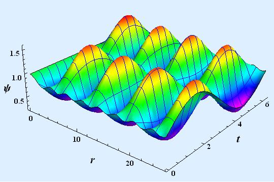
Figure 1: Stationary spherically symmetric monopole solution in the numeric domain $(0\leq r\leq 8\pi,~{}0\leq t\leq 2\pi)$, $c_{0}=-0.251$, $a_{0}=0.84175$, $A_{0}=0.6405$.

Note that at far distance $r_{f}$ after space-time averaging over the ring $(r_{f}\leq r\leq r_{f}+2\pi,0\leq t\leq 2\pi)$ one gains a partial screening effect for the monopole charge. The obtained numeric solution implies an averaged monopole charge at distance $r_{f}=30$

$$g_{\rm m} = \dfrac{1}{4\pi}\int{\rm d}\theta\,{\rm d}\varphi\,H_{\theta\varphi}=\dfrac{1}{4\pi}\int{\rm d}\theta\,{\rm d}\varphi\,\big{(}\langle\psi^{2}\rangle-1\big{)}\sin\theta$$ (37)

$$= 0.195\cdots,$$

with

$$\langle\psi^{2}\rangle = \dfrac{1}{4\pi^{2}}\int_{r_{f}}^{{r_{f}}+2\pi}{\rm d}r\int_{0}^{2\pi}{\rm d}t\,\psi^{2}(r,t).$$

The space-time averaged magnetic flux of the radial color magnetic field $H_{\theta\varphi}^{3}$ through a sphere does not vanish in general and depends on the radius of the sphere. There is a special non-trivial solution with the parameters $a_{0}=0.1\cdots,\,A_{0}=1.989\cdots$ which corresponds to a totally screened averaged monopole charge.

With a given numeric monopole solution one can verify the quantum stability of the monopole field in a similar manner as we considered in the previous section. One should solve the following Schrödinger type eigenvalue equation for possible unstable modes (the space indices $(m,n=1,2,3)$ correspond to the spherical coordinates $(r,\theta,\varphi)$ respectively)

$$K_{mn}^{ab}\Psi_{n}^{b}(r,\theta,\varphi,t)=\lambda\Psi_{m}^{a}(r,\theta,\varphi,t),$$ (38)

where $\Psi_{n}^{b}(r,\theta,\varphi,t)$ are the wave functions describing the quantum gluon fluctuations, and $K_{mn}^{ab}$ is a differential matrix operator corresponding to one-loop gluon contribution to the effective action in the temporal gauge

$$K_{mn}^{ab} = -\delta^{ab}g_{mn}\partial_{t}^{2}-g_{mn}({\mathscr{D}}_{n}{\mathscr{D}}_{n})^{ab}+2\epsilon^{ab}{}_{c}\mathscr{F}_{mn}^{c}.\qquad$$ (39)

The Schrödinger type equation (38) represents a system of nine non-linear partial differential equations which should be solved on three-dimensional numeric domain with sufficiently high numeric accuracy. An additional technical difficulty in numeric calculation is that one must solve the equations with changing the size of the numeric domain in radial direction in the limit $r\rightarrow\infty$ to verify that all eigenvalues remain positive. Fortunately, the numeric analysis of the solutions corresponding to the lowest eigenvalue is simplified drastically due to factorization property of the original equation (38) and special feature of the class of ground state solutions as we will see below.

The equation (38) in component form admits factorization, it can be written as two decoupled systems of partial differential equations as follows (for brevity of notation we set $g=1$ since the coupling constant can be absorbed by the monopole function $\psi$)

$$(I): (\hat{\Delta}\Psi)_{2}^{2}-\dfrac{2}{r^{2}}\partial_{\theta}\Psi_{1}^{2}+\dfrac{1}{r^{2}}\Big{(}(\psi^{2}-1)\Psi_{2}^{2}-2\psi^{2}\Psi_{3}^{1}+2\csc^{2}\theta(\Psi_{2}^{2}+\Psi_{3}^{1})+2\cot\theta\psi\Psi_{3}^{3}\Big{)}=\lambda\Psi_{2}^{2},$$ (40)

$$(\hat{\Delta}\Psi)_{3}^{1}-\dfrac{2}{r^{2}}\psi\partial_{\theta}\Psi_{3}^{3}+\dfrac{1}{r^{2}}\Big{(}\psi^{2}(-2\Psi_{2}^{2}+\Psi_{3}^{1})-\Psi_{3}^{1}+2\csc^{2}\theta(\Psi_{2}^{2}+\Psi_{3}^{1})+2\cot\theta\Psi_{1}^{2}\Big{)}=\lambda\Psi_{3}^{1},$$

$$(\hat{\Delta}\Psi)_{1}^{2}+\dfrac{2}{r^{2}}\partial_{\theta}\Psi_{2}^{2}+\dfrac{1}{r^{2}}\Big{(}(\cot^{2}\theta+\psi^{2})\Psi_{1}^{2}+2\cot\theta(\Psi_{2}^{2}+\Psi_{3}^{1})+2\psi\Psi_{3}^{3}+2\Psi_{1}^{2}\Big{)}-\dfrac{2}{r}\partial_{r}\psi\Psi_{3}^{3}=\lambda\Psi_{1}^{2},$$

$$(\hat{\Delta}\Psi)_{3}^{3}+\dfrac{2}{r^{2}}\psi\partial_{\theta}\Psi_{3}^{1}+\dfrac{1}{r^{2}}\Big{(}2\psi\Psi_{1}^{2}+2\cot\theta\psi(\Psi_{2}^{2}+\Psi_{3}^{1})+2\psi^{2}\Psi_{3}^{3}+\csc^{2}\theta\Psi_{3}^{3}\Big{)}-\dfrac{2}{r}\partial_{r}\psi\Psi_{1}^{2}=\lambda\Psi_{3}^{3},$$

$$(II): (\hat{\Delta}\Psi)_{1}^{1}+\dfrac{2}{r^{2}}\partial_{\theta}\Psi_{2}^{1}-\dfrac{2}{r^{2}}\psi\partial_{\theta}\Psi_{1}^{3}+\dfrac{1}{r^{2}}\Big{(}(2+\cot^{2}\theta+\psi^{2})\Psi_{1}^{1}+2\psi\Psi_{2}^{3}-2\cot\theta(\Psi_{3}^{2}-\Psi_{2}^{1})\Big{)}$$ (41)

$$-\dfrac{2}{r}\partial_{r}\psi\Psi_{2}^{3}=\lambda\Psi_{1}^{1},$$

$$(\hat{\Delta}\Psi)_{2}^{3}-\dfrac{2}{r^{2}}\partial_{\theta}\Psi_{1}^{3}+\dfrac{2}{r^{2}}\psi\partial_{\theta}\Psi_{2}^{1}+\dfrac{1}{r^{2}}\Big{(}2\psi\Psi_{1}^{1}+2\cot\theta\psi(\Psi_{2}^{1}-\Psi_{3}^{2})+(2\psi^{2}+\csc^{2}\theta)\Psi_{2}^{3}\Big{)}$$

$$-\dfrac{2}{r}\partial_{r}\psi\Psi_{1}^{1}=\lambda\Psi_{2}^{3},$$

$$(\hat{\Delta}\Psi)_{2}^{1}-\dfrac{2}{r^{2}}\partial_{\theta}\Psi_{1}^{1}-\dfrac{2}{r^{2}}\psi\partial_{\theta}\Psi_{2}^{3}+\dfrac{1}{r^{2}}\Big{(}-2\psi\Psi_{1}^{3}+\psi^{2}(\Psi_{2}^{1}+2\Psi_{3}^{2})+2\csc^{2}\theta(\Psi_{2}^{1}-\Psi_{3}^{2})-\Psi_{2}^{1}\Big{)}$$

$$+\dfrac{2}{r}\partial_{r}\psi\Psi_{1}^{3}=\lambda\Psi_{2}^{1},$$

$$(\hat{\Delta}\Psi)_{1}^{3}+\dfrac{2}{r^{2}}\partial_{\theta}\Psi_{2}^{3}+\dfrac{2}{r^{2}}\psi\partial_{\theta}\Psi_{1}^{1}+\dfrac{1}{r^{2}}\Big{(}2\cot\theta\psi\Psi_{1}^{1}+2(1+\psi^{2})\Psi_{1}^{3}-2\psi(\Psi_{2}^{1}+\Psi_{3}^{2})+2\cot\theta\Psi_{2}^{3}\Big{)}$$

$$+\dfrac{2}{r}\partial_{r}\psi(\Psi_{2}^{1}+\Psi_{3}^{2})=\lambda\Psi_{1}^{3},$$

$$(\hat{\Delta}\Psi)_{3}^{2}+\dfrac{1}{r^{2}}\Big{(}2\cot\theta(\psi\Psi_{2}^{3}-\Psi_{1}^{1})-2\psi\Psi_{1}^{3}+\psi^{2}(2\Psi_{2}^{1}+\Psi_{3}^{2})-2\csc^{2}\theta(\Psi_{2}^{1}-\Psi_{3}^{2})-\Psi_{3}^{2}\Big{)}$$

$$+\dfrac{2}{r}\partial_{r}\psi\Psi_{1}^{3}=\lambda\Psi_{3}^{2},$$

where

$$\hat{\Delta}\Psi_{m}^{a}\equiv-(\partial^{2}_{t}+\partial^{2}_{r}+\dfrac{2}{r}\partial_{r}+\dfrac{1}{r^{2}}\partial^{2}_{\theta}+\dfrac{\cot\theta}{r^{2}}\partial_{\theta})\Psi_{m}^{a}.$$

To solve numerically the systems of equations (I), (II), we choose a rectangular three-dimensional domain $(0\leq t\leq 2\pi,r_{0}\leq r\leq L,0\leq\theta\leq\pi)$ and use a simple interpolating function for the monopole solution $\psi(r,t)$

$$\psi^{\rm int} = 1-\dfrac{(1-a_{0})r^{2}}{1+r^{2}}$$ (42)

$$+A_{0}(1-{\rm e}^{-d_{0}r^{2}})\cos(Mr+b_{0})\sin(Mt),\quad$$

where $d_{0}$ and $b_{0}$ are fitting parameters. An obtained numeric solution to the system of equations (I), $(\ref{eqI})$, implies that the lowest eigenvalue is positive, $\lambda_{\rm I}=0.0531$, and the corresponding eigenfunctions have the following properties: the functions $\Psi_{1}^{2}$ and $\Psi_{3}^{3}$ vanish identically, and remaining two functions are related by the constraint $\Psi_{3}^{1}=-\Psi_{2}^{2}$. So that there is only one independent non-vanishing eigenfunction which can be chosen as $\Psi_{2}^{2}$. An important feature of the solution corresponding to the lowest eigenvalue is that the eigenfunction $\Psi_{2}^{2}$ does not depend on the polar angle, Fig.2.

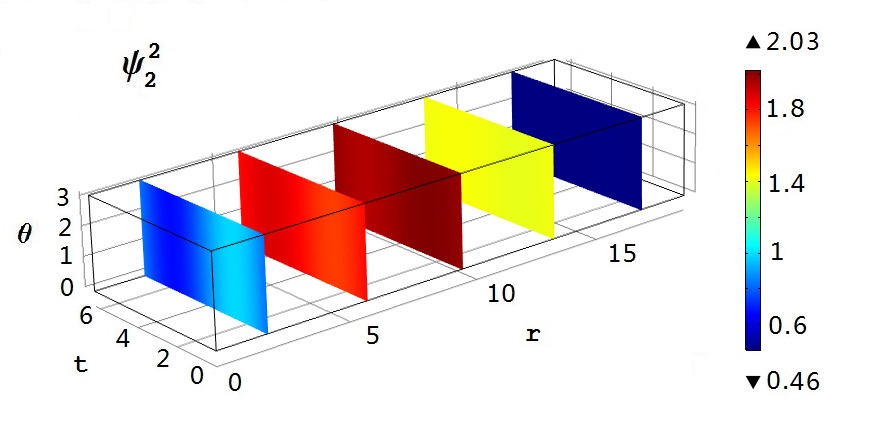
Figure 2: Eigenfunction $\Psi_{2}^{2}$ for the ground state with the lowest eigenvalue $\lambda_{I}=0.0531$, $a_{0}=0.895,~{}A_{0}=0.615$, $g=1$, $M=1$, $0\leq r\leq 6\pi$,  $0\leq t\leq 2\pi$, $0\leq\theta\leq\pi$.

This allows to simplify the system of equations (I) in the case of solutions corresponding to the lowest eigenvalues. One can easily verify that system of equations (I), (40), reduces to one partial differential equation on two-dimensional space-time

$$\Big{(}-\partial^{2}_{t}-\partial^{2}_{r}-\dfrac{2}{r}\partial_{r}+\dfrac{1}{r^{2}}(3\psi^{2}-1)\Big{)}\Psi_{2}^{2}=\lambda\Psi_{2}^{2}.$$ (43)

The last equation represents a simple Schrödinger type equation for a quantum mechanical problem. The equation does not admit negative eigenvalues if the parameter $a_{0}$ of the monopole solution satisfies the condition $a_{0}\geq 1/\sqrt{3}\simeq 0.577\cdots$ which provides a totally repulsive quantum mechanical potential in this equation.

A structure of the system of equations (II) admits similar factorization properties on the space of ground state solutions. We have solved numerically the equations (II), (41), with the same background monopole function $\psi(r,t)$ for various values of the parameters $a_{0},A_{0},M$. In a special case, $a_{0}=0.895,~{}A_{0}=0.615$, $0\leq r\leq 6\pi$ the obtained numeric solution for the ground state has a lowest eigenvalue $\lambda_{\rm II}=0.0142$ which is less than $\lambda_{\rm I}$. All components of the solution do not have dependence on the polar angle and satisfy the following relationships: $\Psi_{2}^{1}=\Psi_{3}^{2}$ and $\Psi_{1}^{1}=\Psi_{2}^{3}=0$. There are two independent non-vanishing functions which can be chosen as $\Psi_{1}^{3}$ and $\Psi_{3}^{2}$. One can check that on the space of solutions corresponding to the lowest eigenvalue the system of equations (II), (41), reduces to two coupled partial differential equations for two functions $\Psi_{1}^{3}(r,t)$ and $\Psi_{3}^{2}(r,t)$

$$(-\partial^{2}_{t}-\partial^{2}_{r}-\dfrac{2}{r}\partial_{r})\Psi_{1}^{3}+\dfrac{2}{r^{2}}\Big{(}(1+\psi^{2})\Psi_{1}^{3}-2\psi\Psi_{3}^{2}\Big{)}$$

$$+\dfrac{4}{r}\partial_{r}\psi\Psi_{3}^{2}=\lambda\Psi_{1}^{3},$$

$$(-\partial^{2}_{t}-\partial^{2}_{r}-\dfrac{2}{r}\partial_{r})\Psi_{3}^{2}+\dfrac{1}{r^{2}}\Big{(}(3\psi^{2}-1)\Psi_{3}^{2}-2\psi\Psi_{1}^{3}\Big{)}$$

$$+\dfrac{2}{r}\partial_{r}\psi\Psi_{1}^{3}=\lambda\Psi_{3}^{2}.$$ (44)

Exact numeric solution profiles for the functions $\Psi_{1}^{3},\Psi_{3}^{2}$ are shown in Fig.3.

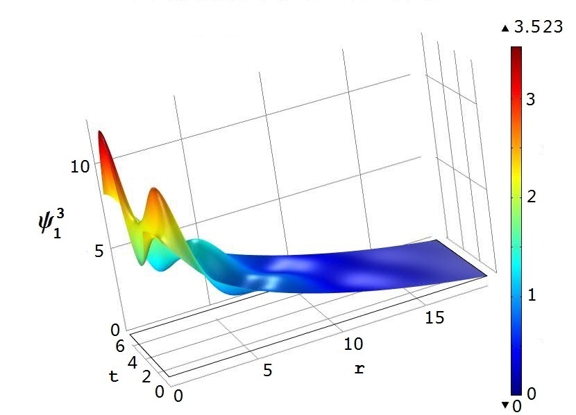
(a)   $\Psi_{1}^{3}$

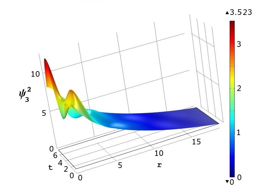
(b)   $\Psi_{3}^{2}$

Figure 3: Solutions to Eqs. (44): the functions $\Psi_{1}^{3}(r,t),~{}\Psi_{3}^{2}(r,t)$ corresponding to the eigenvalue $\lambda=0.014218$, , $a_{0}=0.895,~{}A_{0}=0.615$, $M=1$, $0\leq r\leq 6\pi$,  $0\leq t\leq 2\pi$: (a)$\Psi_{1}^{3}(r,t)$ , (b)  $\Psi_{2}^{1}(r,t)=\Psi_{3}^{2}(r,t)$.

We have obtained that the lowest eigenvalue is positive when the asymptotic monopole amplitude $A_{0}$ is less than a critical value $a_{\rm 1cr}\simeq 0.625$.

We conclude, a ground state solution with the lowest eigenvalue satisfying the original eigenvalue equation (38) can be found by solving a simple system of partial differential equations (44). Note that the numeric solving of the original eigenvalue equations (38) on a three-dimensional space-time does not provide high enough accuracy, especially in the case of large radial size of the numeric domain. This causes difficulty in studying the positiveness of the eigenvalue spectrum in the limit of infinite space when the eigenvalues become very close to zero. Solving the reduced two-dimensional partial differential equations (44) can be performed easily using standard numeric packages with a high enough numeric accuracy and convergence. The obtained numeric accuracy for the eigenvalues $\lambda(L)$ in solving the two-dimensional equations (44) is $1.0\times 10^{-5}$ which allows to construct the eigenvalue dependence on the radial size $L$ of the space-time domain in the range $6\pi\leq L\leq 64\pi$. We have proved that the lowest eigenvalue $\lambda(L)$ approaches zero with increasing $L$ from positive values, as it is shown in Fig.4.

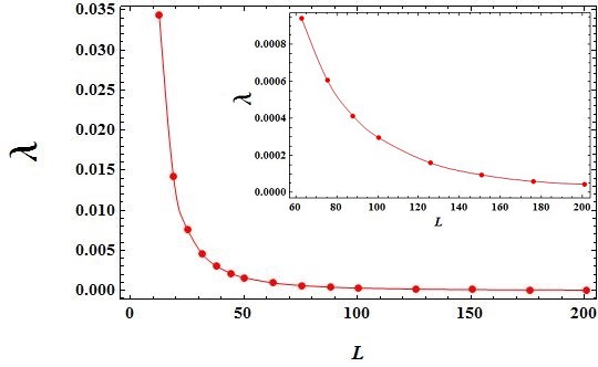
Figure 4: Lowest eigenvalue dependence, $\lambda(L)$, on the radial size $L$ of the numeric domain.

This implies that the ground state solution describes the main mode of the standing spherical wave with a wave vector proportional to the inverse of radial size of the box, $|\vec{p}|\simeq 1/L$. This completes the proof of quantum stability of the spherically symmetric stationary monopole solution.

The stationary single monopole solution represents a simple example of a spherically symmetric vacuum field which has a non-trivial intrinsic microscopic structure determined by two parameters, the amplitude $A_{0}$ and frequency $M$ of space-time oscillations of the monopole field. Quantum mechanical consideration implies that the frequency of vacuum monopole field oscillations has a finite minimal value. One can estimate a lower bound of $M$ using the condition that the characteristic length $\lambda=2\pi/M$ of the monopole field should be less than the hadron size. At macroscopic scale, when the observation time is much larger than the period of oscillations of the stationary monopole solution, the vacuum averaged value of the gauge potential, $\langle 0|A_{\mu}^{a}|0\rangle$, vanishes as it should be in the confinement phase. Contrary to this, the so-called vacuum gluon (monopole) condensate $H^{2}\equiv\langle 0|\vec{F}_{\mu\nu}^{2}|0\rangle$ does not vanish after averaging over time, and it has inhomogenious distribution inside the hadron. Calculation of an exact effective action in the case of inhomogeneous background vacuum fields represents unresolved problem. In the weak field approximation one can apply the known expression for the Savvidy renormalized one-loop effective potential savv ; yildiz80 ; claudson80 ; adler81 ; dittrich83 ; flory83 ; blau91 ; reuter97 ; chopakPRD

$$V_{\rm eff}(H)=\dfrac{1}{4}H^{2}+\dfrac{11g^{2}(\mu)}{96\pi^{2}}H^{2}\Big{(}\ln\dfrac{g(\mu)H}{\mu^{2}}-\dfrac{3}{2}\,\Big{)},$$ (45)

where $g(\mu)$ is a renormalized coupling constant defined at the subtraction point $\mu^{2}\simeq\Lambda_{\rm QCD}$ ($\alpha_{s}=g^{2}(\mu)/(4\pi)\simeq 1$). For qualitative estimates we replace the vacuum spherically symmetric monopole field $H^{2}$ with its mean value $\overline{H^{2}}$ obtained by averaging over the space and time. The potential $V_{\rm eff}(\bar{H})$ has a non-trivial minimum corresponding to a negative vacuum energy density at non-zero value of the averaged monopole field, $\bar{H}_{0}\simeq 0.138\mu^{2}$ chopakPRD . The value $\bar{H}_{0}$ is consistent with the frequency and amplitude values $(M\simeq 1,A_{0}\leq a_{1cr})$ corresponding to stable stationary monopole field configurations.

One should stress that the generation of a non-trivial vacuum originates from the magnetic moment interaction between the vacuum magnetic field and quantum gluon fluctuations. Such an interaction induces the vacuum energy decrease for sufficiently small values of the vacuum monopole condensate parameter $\bar{H}$. In the case of the spherically symmetric monopole solution our numeric analysis confirms that for large values of parameters $M,A_{0}$, i.e., for large values of $\bar{H}_{0}$, the monopole field obtains quantum instability which prevents the generation of a stable monopole condensate.

V Discussion

We have demonstrated that there is a subclass of stationary spherically symmetric monopole solutions which possesses quantum stability for restricted values of the amplitude $A_{0}$ of the asymptotic monopole solution, (34). Recently it has been found that there is another stable stationary monopole-antimonopole solution in $SU(2)$ and $SU(3)$ QCD P4 . This gives a hope that a true vacuum can be formed through condensation of such monopoles and/or monopole-antimonopole pairs.

Existence of stable monopole field configurations and possible formation of a gauge invariant vacuum monopole condensate may shed light on the origin of color confinement in QCD and give a partial answer to a simple but puzzling question: why do we have the spontaneous symmetry breaking in the electroweak theory, while in QCD the color symmetry is preserved despite the similar gauge group structure in both theories? The vanishing vacuum averaged value of the gluon field operator corresponding to the stationary monopole solution, $\langle A_{m}^{a}\rangle$, testifies that there is no spontaneous symmetry breaking in QCD in the confinement phase. One can apply the ansatz (29) to electroweak gauge potentials corresponding to the group $SU(2)\times U_{Y}(1)$ of the Weinberg-Salam model to find similar stationary electroweak monopole solutions. One considers the Higgs complex doublet $\Phi$ in the unitary gauge, and choose a simple Dirac monopole ansatz for the hypermagnetic field $\mathscr{B}_{\mu}$

$$\Phi=\left(\begin{array}[]{cc}0\\ \rho(r,t)\end{array}\right),\qquad\mathscr{B}_{\mu}=\cos\theta.$$ (48)

Direct substitution of the ansatz (29) and the last equations (48) into the equations of motion of the Weinberg-Salam model results in two equations for two functions $\psi(r,t),~{}\rho(r,t)$

$$\begin{array}[]{rcl}\partial^{2}_{t}\psi-\partial^{2}_{r}\psi+\dfrac{1}{2}\psi\rho^{2}+\dfrac{1}{r^{2}}(\psi^{2}-1)&=&0,\\ \partial_{t}^{2}\rho-\partial^{2}_{r}\rho-\dfrac{2}{r^{2}}\partial_{r}\rho+\dfrac{1}{2r^{2}}\rho\psi^{2}+\kappa\rho(\rho^{2}-1)&=&0,\end{array}$$ (49)

where $\kappa$ is the coupling constant of the Higgs potential. In a special case of static field configurations the equations (49) reduce to the ordinary differential equations describing a known Cho-Maison monopole chomaison . A simple numeric analysis of the equations (49) shows that a non-static generalization of the Cho-Maison monopole exists, however it has the same singularity at the origin $r=0$. We conclude that there is a principal difference between the Weinberg-Salam model and QCD: the absence of a regular monopole solution in the Weinberg-Salam model implies that there is no generation of a stable monopole condensation like in QCD. This leads to non-vanishing vacuum averaged values for the gauge bosons and, consequently, to the spontaneous symmetry breaking. Contrary to this, in QCD, in the confinement phase, the mean value of the monopole field $\langle 0|A_{m}^{a}|0\rangle$ averaged over the periodic space-time domain vanishes, so that the color symmetry is exact.

In conclusion, we have demonstrated that a classical stationary spherically symmetric monopole solution provides a stable vacuum field configuration in a pure $SU(2)$ QCD. Generalization of our results to the case of $SU(3)$ QCD is presented in a separate paper Pa1 . The possibility that a stationary classical solution can be related to vacuum structure is not much surprising since it was noticed in the past that color magnetic flux tubes in the “spaghetti” vacuum should be vibrating from the quantum mechanical consideration olesen81 . An unexpected result is that a stationary color monopole solution exists in a pure QCD without any matter fields, and it possesses remarkable features such as the finite energy density, total zero spin and existence of intrinsic mass scale parameter. This gives a strong indication to generation of a stable vacuum condensate in QCD.

Appendix A Variational analysis of quantum stability of the stationary monopole field

To reveal the origin of stability of our numeric solution we undertake analytic study of the eigenvalue spectrum of the Schrödinger type equation (38). Since we are interested only in the lowest eigenvalue solution, one can solve approximately the equation (38) by applying variational methods. Within the framework of the variational approach one has to minimize the following “energy” functional

$${\mathscr{H}}=\int{\rm d}r\,{\rm d}\theta\,{\rm d}\varphi\,{\rm d}t\,r^{2}\!\sin\theta\,\Psi_{m}^{a}K_{mn}^{ab}\Psi_{n}^{b}.$$ (50)

The structure of the kinetic operator $K_{mn}^{ab}$ and the finiteness condition of the functional ${\mathscr{H}}$ allow to fix the singularities along the boundaries $\theta=0$ and $\theta=\pi$ in the integral density in (50). We factorize the angle dependence of the ground state wave functions using the leading order approximation in Fourier series expansion for the functions $f_{m}^{a}$ as follows

$$\Psi_{1}^{3}(r,\theta,\varphi,t)=f_{1}^{3}(r,t),$$ (51)

and for other functions

$$\Psi_{m}^{a}(r,\theta,\varphi,t) = f_{m}^{a}(r,t)\sin\theta.$$ (52)

With this one can perform the integration in (50) over the angle variables $(\theta,\varphi)$ and obtain an effective “energy” functional

$${\mathscr{H}}^{\rm eff} = \int{\rm d}r\,{\rm d}t\,r^{2}f_{m}^{a}K_{mn}^{ab}f_{n}^{b}$$

$$= \int{\rm d}r\,{\rm d}t\,r^{2}f_{m}^{a}\big{[}g_{mn}\delta^{ab}\tilde{K}_{0}+V_{mn}^{ab}(r,t)\big{]}f_{n}^{b},$$

where $\tilde{K}_{0}=-\partial^{2}_{t}-\partial^{2}_{r}-(2/r)\partial_{r}$, and $V_{mn}^{ab}$ is an effective potential. The quadratic form

$$\langle f|V|f\rangle\equiv\sum_{m,n,a,b}f_{m}^{a}V_{mn}^{ab}f_{n}^{b}$$ (54)

contains terms with radial dependencies proportional to $(1/r^{2})$ and $(1/r)$ which correspond to the centrifugal and Coulomb like potentials, respectively. In the case of a pure Wu-Yang monopole it was shown that such a background field leads to the vacuum instability due to the appearance of the attractive potential $(-1/r^{2})$ in the respective eigenvalue equation for unstable modes pak05 . In our case, in the presence of the stationary monopole solution, one can verify that due to the structure of the local solution near $r=0$ in equation (35) the quadratic form containing the terms proportional to $(1/r^{2})$ is positively defined for any smooth fluctuating functions $f_{m}^{a}(r,t)$ satisfying the finiteness condition of the “energy” functional. This provides a non-vanishing positive centrifugal potential in the corresponding Schrödinger equation which prevents appearance of negative eigenmodes for a special class of background monopole solutions.

By variation of the functional ${\mathscr{H}}^{\rm eff}$ with respect to functions $f_{m}^{a}(r,t)$, one obtains the following effective Schrödinger type equation

$$K_{mn}^{ab}f_{n}^{b}(r,t)=\lambda f_{m}^{a}(r,t).$$ (55)

The obtained system of nine differential equations is explicitly factorized into four decoupled systems of partial differential equations

$$(I): \tilde{K}_{0}f_{2}^{2}+\dfrac{1}{r^{2}}\big{(}(5+2\psi^{2})f_{2}^{2}+(6-4\psi^{2})f_{3}^{1}\big{)}=\lambda f_{2}^{2},$$

$$\tilde{K}_{0}f_{3}^{1}+\dfrac{1}{r^{2}}\big{(}(6-4\psi^{2})f_{2}^{2}+(5+2\psi^{2})f_{3}^{1}\big{)}=\lambda f_{3}^{1},$$

$$(II): \tilde{K}_{0}f_{1}^{2}+\dfrac{1}{r^{2}}(3+\psi^{2})f_{1}^{2}+2\psi f_{3}^{3})-\dfrac{2\psi^{\prime}}{r}f_{3}^{3}=\lambda f_{1}^{2},$$

$$\tilde{K}_{0}f_{3}^{3}+\dfrac{2}{r^{2}}((1+\psi^{2})f_{3}^{2}+\psi f_{1}^{2})-\dfrac{2\psi^{\prime}}{x}f_{1}^{2}=\lambda f_{3}^{3},$$

$$(III): \tilde{K}_{0}f_{2}^{1}+\dfrac{1}{r^{2}}((10+4\psi^{2})f_{2}^{1}-(12-8\psi^{2})f_{3}^{2}$$ (58)

$$-3\pi\psi f_{1}^{3})+\dfrac{3\pi\psi^{\prime}}{r}f_{1}^{3}=\lambda f_{2}^{1},$$

$$\tilde{K}_{0}f_{1}^{3}+\dfrac{1}{2r^{2}}(4(1+\psi^{2})f_{1}^{3}-\pi\psi(f_{2}^{1}+f_{3}^{2}))$$

$$+\dfrac{\pi\psi^{\prime}}{2r}(f_{2}^{1}+f_{3}^{2})=\lambda f_{1}^{3},$$

$$\tilde{K}_{0}f_{3}^{2}+\dfrac{1}{4r^{2}}(2(5f_{3}^{2}-6f_{2}^{1})+4\psi^{2}(2f_{2}^{1}+f_{3}^{2})$$

$$-3\pi\psi f_{1}^{3})+\dfrac{3\pi\psi^{\prime}}{4r}f_{1}^{3}=\lambda f_{3}^{2}\,,$$

The remaining system (IV) of two equations for the functions $f_{1}^{1},f_{2}^{3}$ is the same as the system (II) for the functions $f_{1}^{2},f_{3}^{3}$ with the replacement $f_{1}^{2}\rightarrow f_{1}^{1}$, $f_{3}^{3}\rightarrow f_{2}^{3}$. The obtained equations represent Schrödinger type equations for a charged particle with a positive centrifugal potential and oscillating Coulomb potential. It is clear that solutions $\psi(r,t)$ with small enough parameters $a_{0},A_{0}$ will imply a positive eigenvalue spectrum since the potential with a small enough depth and asymptotic behavior, ${\mathscr{O}}(1/r^{\alpha})$ and $(\alpha\leq 1)$, does not lead to bound states in the case of space dimension $d\geq 3$.

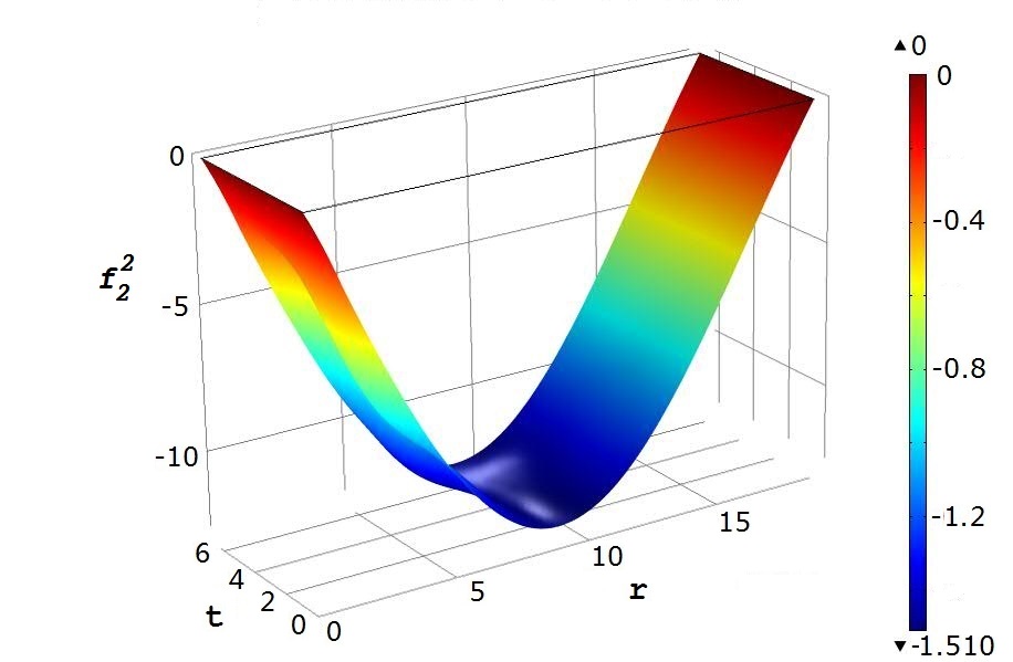
Figure 5: Solution $f_{2}^{2}$ to Eq. (I), $f_{3}^{1}(r,t)=-f_{2}^{2}(r,t)$; $\lambda_{I}=0.0586$, $0\leq r\leq 6\pi$,  $0\leq t\leq 2\pi$.

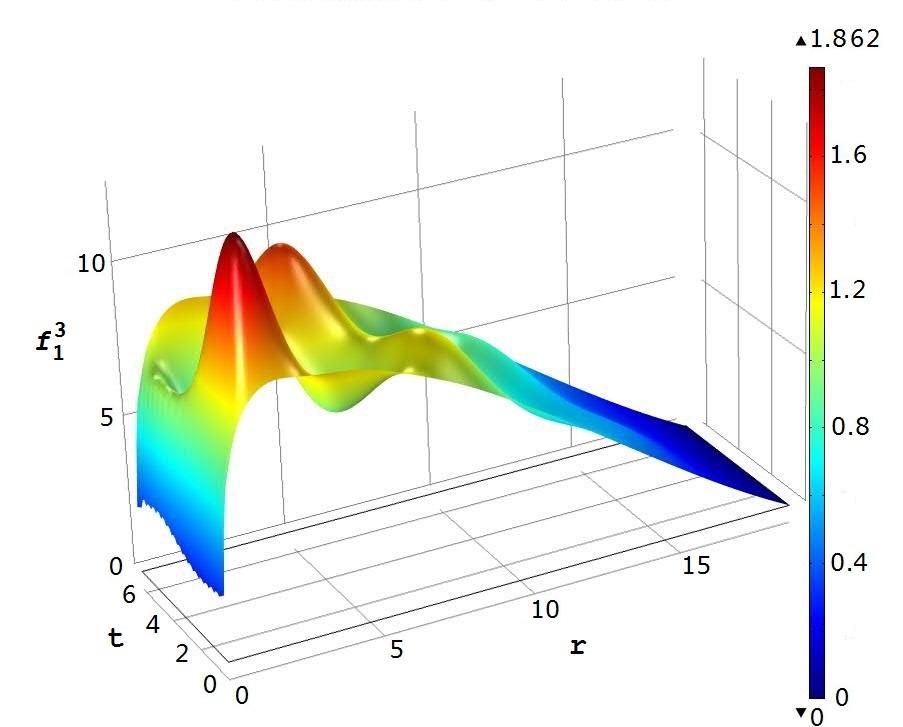
(a)  

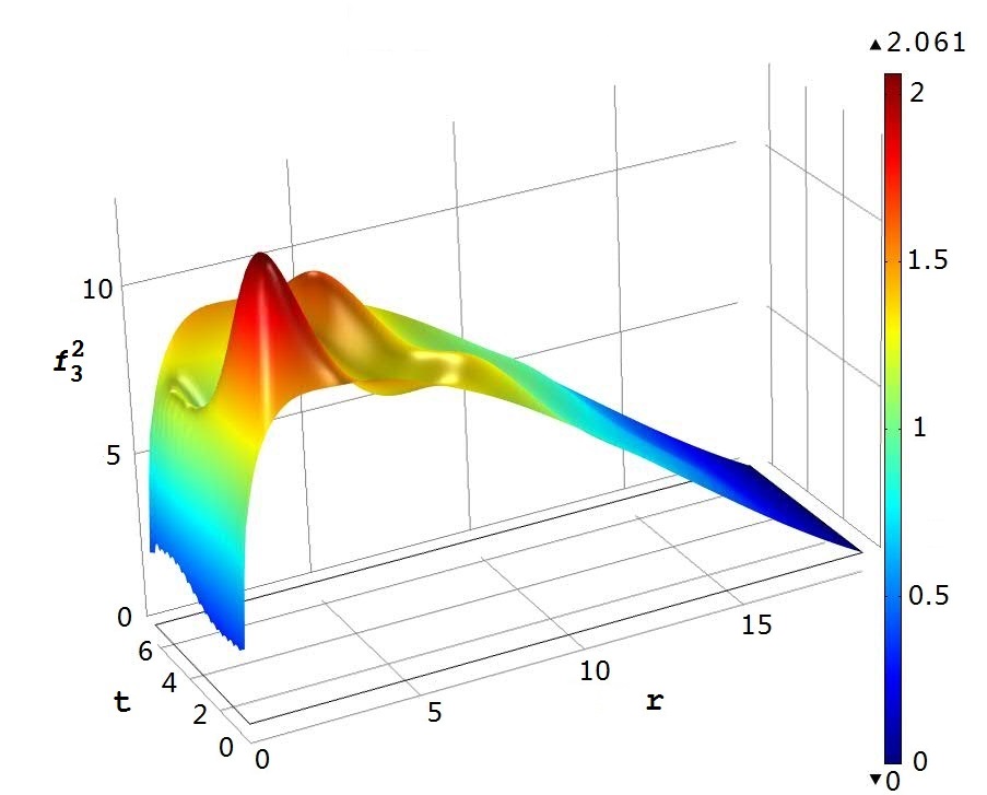
(b)  

Figure 6: Solution to Eq. (III) $\lambda=0.0293$, $0\leq r\leq 6\pi$,  $0\leq t\leq 2\pi$: (a) $f_{1}^{3}(r,t)$, (b) $f_{2}^{1}(r,t)=f_{3}^{2}(r,t)$.

Substituting the interpolating function (42) into the Schrödinger equations, one can solve them and obtain the eigenvalue spectrum. Numeric analysis shows that a complete positive eigenvalue spectrum exists for solutions $\psi(r,t)$ with parameter values of $a_{0}$ in a finite range $0.89\leq a_{0}\leq 1$. We solve the equations (I-III) for a case of a monopole background field specified by the parameters $a_{0}=0.895,~{}A_{0}=0.615$. A typical profile function for the solutions to equations (I) and (II) has weak dependence on time, Fig.5. The corresponding ground state eigenvalues are close to each other, $\lambda_{\rm I}\simeq 0.0586,~{}\lambda_{\rm II}\simeq 0.0552$. The solution to equation (III) has a lower eigenvalue $\lambda_{\rm III}\simeq 0.0293$ and manifests larger time fluctuations as it is shown in Fig.6. Note that the principal lowest eigenvalue originates from the decoupled system of equations (III) for the functions $f_{2}^{1},f_{1}^{3}$ and $f_{3}^{2}$ in qualitative agreement with the results of exact numerical solving the original eigenvalue equation presented in Section IV.

References

- (1) S.J. Brodsky, G.F. de Teramond, and H.G. Dosch, Int. J. Mod. Phys. A29, 1444013 (2014).
- (2) Y. Nambu, Phys. Rev. D10, 4262 (1974).
- (3) S. Mandelstam, Phys. Rep. 23C, 245 (1976).
- (4) A. Polyakov, Nucl. Phys. B120, 429 (1977).
- (5) G. ’t Hooft, Nucl. Phys. B190, 455 (1981).
- (6) Z. Ezawa and A. Iwazaki, Phys. Rev. D25, 2681 (1982).
- (7) T. Suzuki, Prog. Theor. Phys. 80, 929 (1988).
- (8) H. Suganuma, S. Sasaki, and H. Toki, Nucl. Phys. B435, 207 (1995).
- (9) A. Kronfeld, G. Schierholz, and U. Wiese, Nucl. Phys. B293, 461 (1987).
- (10) T. Suzuki and I. Yotsuyanagi, Phys. Rev. D42, 4257 (1990).
- (11) J. Stack, S. Neiman, and R. Wensley, Phys. Rev. D50, 3399 (1994).
- (12) H. Shiba and T. Suzuki, Phys. Lett. B333, 461 (1994).
- (13) G. Bali, V. Bornyakov, M. Müller-Preussker, and K. Schilling, Phys. Rev. D54, 2863 (1996).
- (14) G.K. Savvidy, Phys. Lett. B71, 133 (1977).
- (15) N.K. Nielsen and P. Olesen, Nucl. Phys. B144, 376 (1978).
- (16) H.B. Nielsen and M. Ninomiya, Nucl. Phys. B156, 1 (1979).
- (17) H.B. Nielsen and P. Olesen, Nucl. Phys. B160, 380 (1979).
- (18) J. Ambjørn and P. Olesen, Nucl. Phys. B170, 60 (1980).
- (19) J. Ambjørn and P. Olesen, Nucl. Phys. B170, 265 (1980).
- (20) M. Bordag, Phys. Rev. D67, 065001 (2003).
- (21) Y.M. Cho and D.G. Pak, Phys. Lett. B632, 745 (2006).
- (22) G.H. Derrick, J. Math. Phys. 5, 1252 (1964).
- (23) R. Jackiw, The Yang-Mills Vacuum as a Bloch Wave, preprint MIT-CTP-625, (MIT, LNS). Apr 1977. 12 pp.
- (24) R. Jackiw, Rev. Mod. Phys. 49, 681 (1977).
- (25) G.Z. Baseyan, S.G. Matinyan, and G.K. Savvidy, Pisma Zh. Eksp. Teor. Fiz. 29, 641 (1979); JETP Lett. 29, 587 (1979).
- (26) V. Lahno, R. Zhdanov, and W. Fushchych, J. Nonlinear Math. Phys. 2, 51 (1995).
- (27) A. V. Smilga, Lectures on Quantum Chromodynamics, [arXiv:hep-ph/9901412].
- (28) M. Frasca, Mod. Phys. Lett. A24, 2425 (2009).
- (29) A. Tsapalis, E.P. Politis, X.N. Maintas and F.K. Diakonos, Phys. Rev. D93, 085003 (2016).
- (30) B.-H. Lee, Y. Kim, D.G. Pak, T. Tsukioka, and P.M. Zhang, Int. J. Mod. Phys. A32, 1750062 (2017).
- (31) A. Yildiz and P. Cox, Phys. Rev. D21, 1095 (1980).
- (32) M. Claudson, A. Yilditz, and P. Cox, Phys. Rev. D22, 2022 (1980).
- (33) S. Adler, Phys. Rev. D23, 2905 (1981).
- (34) W. Dittrich and M. Reuter, Phys. Lett. B128, 321, (1983).
- (35) C. Flory, Phys. Rev. D28, 1425 (1983).
- (36) S.K. Blau, M. Visser, and A. Wipf, Int. J. Mod. Phys. A06, 5409 (1991).
- (37) M. Reuter, M.G. Schmidt, and C. Schubert, Ann. Phys. 259, 313 (1997).
- (38) Y.M. Cho and D.G. Pak, Phys. Rev. D65, 074027 (2002).
- (39) V. Schanbacher, Phys. Rev. D26, 489 (1982).
- (40) H. Leutwyler, Nucl. Phys. B179, 129 (1981).
- (41) C. Ragiadakos, Phys. Rev. D26, 1996 (1982); Phys. Lett. B100, 471 (1981).
- (42) R. Parthasarathy, M. Singer, and K.S. Viswanathan, Can. J. Phys. 61, 1442 (1983).
- (43) S. Huang and A.R. Levi, Phys. Rev. D49, 6849 (1994).
- (44) Y.M. Cho and D.G. Pak, Dynamical Symmetry Breaking and Magnetic Confinement in QCD, Procs. of TMU Symp., Tokyo (2000), [arXiv:hep-th/000051].
- (45) E.M. Lifshitz and L.P. Pitaevskii, Statistical Physics, Part 2: Theory of Condensed State, Vol. 9 (1st ed.), Butterworth-Heinemann (1980).
- (46) M. Luscher, Phys. Lett. B70, 321 (1977).
- (47) B. Schechter, Phys. Rev. D16, 3015 (1977).
- (48) H. Arodz, Phys. Rev. D27, 1903 (1983).
- (49) E. Farhi, V.V. Khoze, and R Singleton, Phys. Rev. D47, 5551 (1993).
- (50) A. Abouelsaood and M.H. Emam, Phys. Lett. B412, 328 (1997).
- (51) Y.M. Cho, Phys. Rev. D21, 1080 (1980).
- (52) D.G. Pak, B.-H. Lee, Y. Kim, T. Tsukioka and P.M. Zhang, [arXiv:1703.09635[hep-th]].
- (53) Y.M. Cho and D. Maison, Phys. Lett. B391, 360 (1997).
-
(54)
B.-H. Lee, Y. Kim, D.G. Pak, and T. Tsukioka,
[arXiv:1607.02083[hep-th]]. - (55) P. Olesen, Physica Scripta, 23, 1000 (1981).