Testing the running coupling $k_{T}$-factorization formula for the inclusive gluon production

Abstract

The inclusive gluon production at midrapidities is described in the Color Glass Condensate formalism using the $k_{T}$ - factorization formula, which was derived at fixed coupling constant considering the scattering of a dilute system of partons with a dense one. Recent analysis demonstrated that this approach provides a satisfactory description of the experimental data for the inclusive hadron production in $pp/pA/AA$ collisions. However, these studies are based on the fixed coupling $k_{T}$ - factorization formula, which does not take into account the running coupling corrections, which are important to set the scales present in the cross section. In this paper we consider the running coupling corrected $k_{T}$ - factorization formula conjectured some years ago and investigate the impact of the running coupling corrections on the observables. In particular, the pseudorapidity distributions and charged hadrons multiplicity are calculated considering $pp$, $dAu/pPb$ and $AuAu/PbPb$ collisions at RHIC and LHC energies. We compare the corrected running coupling predictions with those obtained using the original $k_{T}$ - factorization assuming a fixed coupling or a prescription for the inclusion of the running of the coupling. Considering the Kharzeev - Levin - Nardi unintegrated gluon distribution and a simplified model for the nuclear geometry, we demonstrate that the distinct predictions are similar for the pseudorapidity distributions in $pp/pA/AA$ collisions and for the charged hadrons multiplicity in $pp/pA$ collisions. On the other hand, the running coupling corrected $k_{T}$ - factorization formula predicts a smoother energy dependence for $dN/d\eta$ in $AA$ collisions.

I Introduction

The understanding of inclusive hadron production in hadronic collisions is an important challenge for the theory of the strong interactions, since these processes are expected to be dominated by small transverse momentum exchange. In general, nonperturbative approaches and/or phenomenological models based on soft physics (e.g. Reggeon approach) are used to study hadron production with a satisfactory description of the experimental data. However, a shortcoming of these approaches is that they are not based on quarks and gluons and have no clear connection to the Quantum Chromodynamics (QCD). The QCD dynamics at high energies and large nuclei predicts the formation of a new state of matter, called Color Glass Condensate (For a review see Refs. review1 ), characterized by the saturation scale $Q_{s}$, which is the typical momentum scale in the hadron wave function. The presence of this scale, which increases with energy and the atomic number, allows to treat hadron production on a solid theoretical basis, where perturbative methods can be applied. In the last years, the framework of the CGC approach have been used to describe with success the experimental data for the hadron production. In high energy collisions we expect to observe the transition from a linear description of the QCD dynamics, based on the DGLAP dglap and/or BFKL bfkl evolution equations, to a nonlinear description based on the Color Glass Condensate formalism hdqcd . The transition between these two regimes is determined by the saturation scale $Q_{s}$, which grows with the energy and atomic number. In the last years a comprehensive phenomenological analysis has been carried out to understand the HERA, RHIC and LHC data review1 ; hdqcd . Several theoretical studies have improved the CGC formalism by the inclusion of higher order corrections balnlo ; kovnlo ; iancunlo ; lappinlo . In particular, the running coupling corrections to the kernel of the Balitsky - Kovchegov (BK) equation bk were calculated in Refs. balnlo ; kovnlo , with the solution being able to describe several observables at HERA, RHIC and LHC. More recently, the contributions of large single and double transverse momentum logarithms have been resummed to all orders and included in the BK equation iancunlo ; lappinlo , with the resulting evolution equation being stable and generating a physically meaningful evolution of the dipole amplitude. In addition, the formalism of single inclusive hadron production in the framework of the hybrid approach proposed in Ref. dhj has been improved by the inclusion of next-to-leading order (NLO) corrections in Refs. stasto_nlo ; armesto_nlo ; watanabe , and a generalization to higher orders of the $k_{T}$ - factorization formalism for inclusive gluon production was conjectured in Ref.  Kovchegov.Horowitz . As demonstrated in Ref. watanabe , the NLO corrections of the hybrid formalism bring a better agreement of the predictions with the LHC and RHIC data on forward hadron production. In contrast, the impact of the higher order corrections in the $k_{T}$ - factorization formalism on observables is still unknown. This is the subject of the present paper.

The $k_{T}$ - factorization formalism of gluon production in the central rapidity region (where the wave functions of both colliding particles are probed in the small-x regime) has been proposed in Ref. glr and has been derived in the leading $\log(1/x)$ and fixed coupling approximations in Ref. KT , considering the scattering of a dilute parton system on a dense one (See also Ref. braun ). In a series of papers KLN , Kharzeev, Levin and Nardi (KLN) have studied particle production at midrapidities in $pp/pA/AA$ collisions in terms of the $k_{T}$ - factorization formalism. They have assumed that the main properties of hadron production, as for example the energy, rapidity and transverse momentum dependence, are determined in the initial stage of the collision by the interaction between gluons with transverse momentum of the order of the saturation scale $Q_{s}$. The presence of this scale regularizes the infrared behavior of the parton transverse momentum distributions and justifies a perturbative approach to the process. Since the basic predictions of the KLN approach have been qualitatively confirmed by RHIC and LHC data, several authors have improved the KLN formalism in order to obtain a quantitative description of these data. In particular, in Refs. amir ; albadum ; Albacete ; dumitru ; tribedy , different models of the unintegrated gluon distribution and/or distinct treatments of the nuclear geometry have been considered. Although the $k_{T}$ - factorization formula has been derived assuming that $\alpha_{s}$ is a constant, these different phenomenological studies have considered the running of the coupling constant and verified that it leads to an improvement of the agreement between theory and data. However, analysing in more detail these distinct predictions, we can observe that they were obtained using different choices of scale for the running coupling constant. Such uncertainty is expected in a leading order calculation, where the scales of the couplings are not known. Consequently, the inclusion of running coupling corrections in inclusive gluon production is an important step to obtain quantitative predictions with higher accuracy. In Ref.  Kovchegov.Horowitz , the authors have calculated the running coupling corrections for the lowest - order gluon production cross section using the scale - setting prescription due to Brodsky, Lepage and Mackenzie (BLM) blm . They found that the resulting cross section is expressed in terms of seven factors with running couplings, instead of the three present in the fixed coupling calculation. In particular, two of these running couplings run with complex - valued momentum scales, which are complex conjugates of each other, implying real production cross sections. Finally, this calculation fixes the scales of the running coupling constants appearing in the cross section. Based on these results for lowest - order gluon production, the authors have proposed a running coupling corrected $k_{T}$ - factorization formula, which is expected to be valid in the same regime as the original fixed order formula. Although the proof of this formula is still an open question, it is expected that the resulting formula may still be a good approximation for the exact answer. Such expectation motivates the phenomenological analysis performed in this paper. In what follows we will compare the predictions of the running coupling $k_{T}$ - factorization formula with those obtained assuming a fixed coupling constant and two different prescriptions for the inclusion of the running coupling in the leading order formula. In all calculations we will use the same model of the unintegrated gluon distribution and we will use the same prescription for hadronization. Moreover, we will consider a simplified treatment of the nuclear geometry. This procedure allows us to estimate more precisely the impact of the running coupling corrections on the $k_{T}$ - factorization formula. Such aspects surely can and should be improved in a quantitative comparison of the formalism with the experimental data. However, we believe that our main conclusions will not be strongly modified.

This paper is organized as follows. In the next Section we will present a brief review of the $k_{T}$ - factorization formalism and discuss the different prescriptions for the treatment of the coupling constant which will be considered in our analysis. In Section III, the KLN model of the unintegrated gluon distribution will be presented as well as the basic formulas for the calculation of the observables. Moreover, we will compute the pseudo - rapidity and energy distributions measured in hadron production in $pp/pA/AA$ collisions at RHIC and LHC energies. We will use the running coupling $k_{T}$ - factorization formula and compare its predictions with those obtained assuming a fixed coupling constant and two different prescriptions for the inclusion of the running coupling in the leading order formula. Finally, in Section IV we summarize our main conclusions.

II Inclusive gluon production in the $k_{T}$-factorization formalism

In this Section we will discuss inclusive gluon production in the $k_{T}$-factorization formalism. Before presenting the main formulas, a comment is in order. As described in the Introduction, the cross section of this process was proposed in Ref. glr and proven in Ref. KT (See also Ref. braun ) considering the scattering of a dilute partonic system on a dense one at fixed coupling constant and in leading $\log(1/x)$ approximation. Consequently, its application is well justified for gluon production at midrapidity in $pA$ collisions. On the other hand, in the case of $pp$ and $AA$ collisions at high energies, the gluon jet at midrapidities is produced by the interaction of two dense systems. In such cases, factorization breaking effects are expected to become significant raju , modifying the basic $k_{T}$-factorization formulas. However, the magnitude of these corrections is still subject of intense debate and its contribution in the kinematical range probed by the LHC is not well known. The fact that the $k_{T}$-factorization formalism allows us to obtain a very good description of the current data, suggests that these corrections are not large and that this formalism can be considered a reasonable approximation for the treatment of gluon production in $pp$ and $AA$ collisions at central rapidities. Therefore, in what follows, we will apply the $k_{T}$-factorization formalism to $pp$, $pA$ and $AA$ collisions.

Let us consider the production of a gluon with momentum $k_{T}$ at rapidity $y$ in a collision between the hadrons $h_{1}$ and $h_{2}$, with $h_{i}=p$ or $A$. In the $k_{T}$-factorization formalism, the differential cross section for this process will be given by KT

$$\frac{d^{3}\sigma}{d^{2}k_{T}\,dy}\,=\,\frac{2}{C_{F}}\,\frac{1}{{\bm{k}}^{2}}\,\int d^{2}q\,\alpha_{s}\,\phi_{h_{1}}({\bm{q}},y)\,\phi_{h_{2}}({{\bm{k}}-\bm{q}},Y-y)\,,$$ (1)

where $Y$ is the total rapidity interval of the collision, $C_{F}=(N_{c}^{2}-1)/2N_{c}$ and boldface variables denote transverse plane vectors, ${\bm{k}}=k_{T}=(k^{1},k^{2})$. Moreover, $\phi_{h_{i}}(x_{i},\bm{q})$ denotes the so-called unintegrated gluon distribution, which represents the probability to find a gluon with momentum fraction $x_{i}$ and transverse momentum $\bm{q}$ in the hadron $h_{i}$. This distribution can be expressed as follows

$$\phi_{h_{i}}({\bm{k}},y)\,=\,\frac{C_{F}}{\alpha_{s}\,(2\pi)^{3}}\,\int d^{2}b\,d^{2}r\,e^{-i{\bm{k}}\cdot{\bm{r}}}\ \nabla^{2}_{r}\,\mathcal{N}^{G}_{h_{i}}({\bm{r}},{\bm{b}},y)\,\,,$$ (2)

with $\mathcal{N}^{G}_{h_{i}}({\bm{r}},{\bm{b}},y)$ being the dipole - hadron $h_{i}$ forward scattering amplitude for a gluon dipole of transverse size $\bm{r}$ and $\bm{b}$ the impact parameter of the scattering. The behavior of $\mathcal{N}^{G}$ at large rapidities (small - $x$) is directly related to the QCD dynamics at high energies. In the general case, it will be given by the solution of the JIMWLK evolution equation cgc , but in the large-$N_{c}$ limit it can be expressed in terms of the solution of the BK equation bk for the quark dipole - hadron forward scattering amplitude. As the numerical solution of these equations including the impact parameter dependence is still very challenging levin ; stasto_biernat ; berger , in the studies of gluon production using $k_{T}$ - factorization formula the authors have introduced simplifying assumptions about the impact parameter dependence of the phenomenological models for the unintegrated gluon distributions (or about the quark dipole scattering amplitude), which are based on CGC physics and have their parameters constrained by experimental data amir ; albadum ; Albacete ; dumitru ; tribedy .

In the $k_{T}$ - factorization formula, Eq. (1), the cross section is proportional to the coupling constant $\alpha_{s}$, which was assumed to be constant in its derivation. Moreover, $\alpha_{s}$ appears also in the unintegrated gluon distribution, Eq. (2). In the last years, running coupling corrections have been calculated for the BK-JIMWLK evolution equations and this allows us to estimate the contribution of these corrections to $\mathcal{N}^{G}$. However, it is still not clear how to determine the momentum scale in $\alpha_{s}$ in Eq. (2). This has motivated the generalization of Eqs. (1) and (2) by the inclusion of running coupling constant corrections amir ; albadum ; Albacete ; dumitru ; tribedy . In general, these studies assume that the factorized expression is preserved by these corrections and that the coupling constants in Eqs. (1) and (2) depend on different momentum scales. The choice of these scales is arbitrary and we found different choices in the literature. For example, in Ref. amir , the authors assume that $\alpha_{s}=\alpha_{s}(k_{T}^{2})$ in Eq. (1) and $\alpha_{s}=\alpha_{s}(Q^{2}_{s}(x_{i}))$ in Eq. (2). On the other hand, in Ref. Albacete it is assumed that $\alpha_{s}=\alpha_{s}(Q^{2})$ in Eq. (1), with $Q^{2}=\mbox{max}\{k^{2},(k-q)^{2}\}$, and the scale of running coupling in Eq. (2) is assumed to be equal to the transverse momentum of the gluon. A common characteristic of these approaches is that they assume the leading order running coupling

$$\alpha_{s}(Q^{2})=\frac{12\pi}{\beta_{0}\ln(Q^{2}/\Lambda_{QCD}^{2})}\,;\quad\quad\quad\beta_{0}=33-2n_{f}$$ (3)

where $\Lambda_{QCD}$ is a non-perturbative scale and $n_{f}$ is the number of fermions. Moreover, very often a smooth freezing of the coupling at low scales is assumed. For example, in Ref. amir the strong coupling is taken to be $\alpha_{s}(Q^{2})=0.5$ when $Q^{2}\leq 0.8$ GeV². As pointed out in Refs. amir ; Albacete , the inclusion of running coupling corrections improves the description of the experimental data. However, as discussed in detail in Ref. Kovchegov.Horowitz , it is not clear that Eq. (1) will keep its factorized form after the inclusion of these corrections. In order to clarify this aspect, the authors of Kovchegov.Horowitz have estimated the running coupling corrections in lowest-order gluon production cross section, finding that three factors of fixed coupling in lowest-order expression should be replaced by seven running couplings, with the new structure being called the septumvirate of couplings. Two scales of the couplings are complex-valued, but given the structure of the expression, the cross section is real. Moreover, the cross section is symmetric in the parton momentum scales. In Ref. Kovchegov.Horowitz the authors have proposed a generalization of the lowest-order expression to higher-orders, which includes the small-$x$ evolution. They proposed the following expression for the running coupling corrected $k_{T}$ - factorization formula

$$\frac{d^{3}\sigma}{d^{2}k_{T}\,dy}\,=\,\frac{2\,C_{F}}{\pi^{2}}\,\frac{1}{{\bm{k}}^{2}}\,\int d^{2}q\ {\overline{\phi}}_{h_{1}}({\bm{q}},y)\,{\overline{\phi}}_{h_{2}}({\bm{k}}-{\bm{q}},Y-y)\,\frac{\alpha_{s}\left(\Lambda_{\text{coll}}^{2}\,e^{-5/3}\right)}{\alpha_{s}\left(Q^{2}\,e^{-5/3}\right)\,\alpha_{s}\left(Q^{*\,2}\,e^{-5/3}\right)}\,\,,$$ (4)

with the unintegrated gluon distribution functions defined by

$${\overline{\phi}}_{h_{i}}({\bm{k}},y)\,=\alpha_{s}\phi_{h_{i}}({\bm{k}},y)\,=\,\frac{C_{F}}{(2\pi)^{3}}\,\int d^{2}b\,d^{2}r\,e^{-i{\bm{k}}\cdot{\bm{r}}}\ \nabla^{2}_{r}\,\mathcal{N}_{h_{i}}({\bm{r}},{\bm{b}},y)\,.$$ (5)

where $\Lambda_{\text{coll}}^{2}$ is a collinear infrared cutoff and the momentum scale $Q$ is given by

$$\ln\frac{Q^{2}}{\mu_{\overline{\text{MS}}}^{2}}\, =\,\frac{1}{2}\,\ln\frac{{\bm{q}}^{2}\,({\bm{k}}-{\bm{q}})^{2}}{\mu_{\overline{\text{MS}}}^{4}}-\frac{1}{4\,{\bm{q}}^{2}\,({\bm{k}}-{\bm{q}})^{2}\,\left[({\bm{k}}-{\bm{q}})^{2}-{\bm{q}}^{2}\right]^{6}}\,\Bigg{\{}{\bm{k}}^{2}\,\left[({\bm{k}}-{\bm{q}})^{2}-{\bm{q}}^{2}\right]^{3}$$

$$\quad\;\times\,\bigg{\{}\left[\left[({\bm{k}}-{\bm{q}})^{2}\right]^{2}-\left({\bm{q}}^{2}\right)^{2}\right]\,\left[\left({\bm{k}}^{2}\right)^{2}+\left(({\bm{k}}-{\bm{q}})^{2}-{\bm{q}}^{2}\right)^{2}\right]+2\,{\bm{k}}^{2}\,\left[\left({\bm{q}}^{2}\right)^{3}-\left[({\bm{k}}-{\bm{q}})^{2}\right]^{3}\right]$$

$$\quad\;-{\bm{q}}^{2}\,({\bm{k}}-{\bm{q}})^{2}\left[2\,\left({\bm{k}}^{2}\right)^{2}+3\,\left[({\bm{k}}-{\bm{q}})^{2}-{\bm{q}}^{2}\right]^{2}-3\,{\bm{k}}^{2}\,\left[({\bm{k}}-{\bm{q}})^{2}+{\bm{q}}^{2}\right]\right]\,\ln\left(\frac{({\bm{k}}-{\bm{q}})^{2}}{{\bm{q}}^{2}}\right)\bigg{\}}$$

$$+\,i\,\left[({\bm{k}}-{\bm{q}})^{2}-{\bm{q}}^{2}\right]^{3}\,\,\bigg{\{}{\bm{k}}^{2}\,\left[({\bm{k}}-{\bm{q}})^{2}-{\bm{q}}^{2}\right]\,\left[{\bm{k}}^{2}\,\left[({\bm{k}}-{\bm{q}})^{2}+{\bm{q}}^{2}\right]-\left({\bm{q}}^{2}\right)^{2}-\left[({\bm{k}}-{\bm{q}})^{2}\right]^{2}\right]$$

$$\quad\;+{\bm{q}}^{2}\,({\bm{k}}-{\bm{q}})^{2}\,\left({\bm{k}}^{2}\,\left[({\bm{k}}-{\bm{q}})^{2}+{\bm{q}}^{2}\right]-2\,\left({\bm{k}}^{2}\right)^{2}-2\,\left[({\bm{k}}-{\bm{q}})^{2}-{\bm{q}}^{2}\right]^{2}\right)\,\ln\left(\frac{({\bm{k}}-{\bm{q}})^{2}}{{\bm{q}}^{2}}\right)\bigg{\}}$$

$$\quad\;\times\,\sqrt{2\,{\bm{q}}^{2}\,({\bm{k}}-{\bm{q}})^{2}+2\,{\bm{k}}^{2}\,({\bm{k}}-{\bm{q}})^{2}+2\,{\bm{q}}^{2}\,{\bm{k}}^{2}-\left({\bm{k}}^{2}\right)^{2}-\left({\bm{q}}^{2}\right)^{2}-\left[({\bm{k}}-{\bm{q}})^{2}\right]^{2}}\Bigg{\}}\,\,,$$ (6)

with $\mu_{\bar{MS}}^{2}$ being the renormalization scale in the $\bar{MS}$ scheme. Differently from Eq. (1), in the corrected expression all scales in the coupling constants are specified. Moreover, it has the expected behaviours for ${\bm{q}}\rightarrow 0$ and ${\bm{q}}\rightarrow{\bm{k}}$ Kovchegov.Horowitz . In Ref. Kovchegov.Horowitz the authors claim that Eq. (4), like Eq. (1), is valid both in the linear and non-linear regimes of the QCD dynamics. However, as emphasized there, only exact calculations can check the validity of this conjecture. We expect Eq. (4) to be a good approximation for the exact answer. This expectation motivates a phenomenological study using the running coupling corrected $k_{T}$ - factorization formula.

III Results

In this section we will compare the predictions of the running coupling corrected $k_{T}$ - factorization formula, given by Eq. (4) and denoted CF hereafter, with those derived using the original formula, Eq. (1). In the latter, we will calculate the inclusive gluon production cross section assuming a fixed value for the coupling constant (denoted FC), and also assuming that the couplings run according to the prescriptions proposed in Refs. Albacete and amir , denoted hereafter by RC1 and RC2, respectively. In order to clarify the impact of the running coupling corrections in the $k_{T}$ - factorization formula we will make the following approximations: (a) we will disregard the impact parameter dependence of the unintegrated gluon distributions and consider only minimum bias collisions assuming that $A_{eff}=20\,(18.5)$ for Pb (Au); (b) we will assume the validity of the principle of Local Parton - Hadron Duality (LPDH), which implies that the form of the rapidity distribution for the hadron spectrum differs from the gluon spectrum only by a numerical factor. This introduces an effective mass $m_{h}$ (it will be always equal to $0.350$ GeV) which incorporates nonperturbative effects and (c) we will use a single model of the unintegrated gluon distribution, namely the KLN model KLN , which encodes the basic aspects of the nonlinear QCD dynamics, and is given by

$$\phi_{KLN}({\bm{k}},y)\, = \frac{2C_{F}}{3\,\pi^{2}\,\alpha_{s}}\,,\quad k\leq Q_{s}$$ (7)

$$= \frac{2C_{F}}{3\,\pi^{2}\,\alpha_{s}}\frac{Q_{s}^{2}}{k^{2}}\,,\quad k>Q_{s}\,,$$ (8)

where the saturation scale is given by $Q_{s}^{2}=A_{eff}^{1/3}Q_{0}^{2}(x_{0}/x)^{\lambda}$ with $Q_{0}=1$ GeV, $x_{0}=3\times 10^{-4}$ and $\lambda=0.288$ GBW.model . As in previous works KLN ; amir , we will multiply $\phi_{KLN}$ by a factor $(1-x)^{4}$ as prescribed by quark couting rules Brodsky:1973kr ; Matveev:1973ra in order to simulate the behavior of the distribution at large $x$ ($x\rightarrow 1$). All these approximations can and should be improved in a quantitative calculation of the observables. However, we believe that our simplified analysis can help us to get an insight on how the running coupling corrections (included in the $k_{T}$ - factorization formula) change the observables. In what follows we will calculate the inclusive hadron production cross section, which is given by

$$\frac{d^{3}N}{d\eta d^{2}k_{T}}=\frac{K}{\sigma_{s}}\,h(y,k_{T},m_{h})\cdot\frac{d^{3}\sigma}{d^{2}k_{T}\,dy}\,\,,$$ (9)

where $\eta$ is the pseudorapidity and $h(y,k_{T},m_{h})$ is the Jacobian for the conversion from rapidity to pseudorapidity, which is given by

$$h(y,k_{T},m_{h})=\sqrt{1-\frac{m_{h}^{2}}{m_{T}^{2}\cosh^{2}y}}\,,$$ (10)

with $m_{T}^{2}=k_{T}^{2}+m_{h}^{2}$. The $K$-factor incorporates in an effective way the contribution of higher order corrections, of possible effects not included in the CGC formalism and also the uncertainty in the conversion of partons to hadrons. Moreover, $\sigma_{s}$ is the average interaction area. As in previous works amir , we will correct the kinematics due to the presence of the mass scale $m_{h}$, replacing $k_{T}\rightarrow\sqrt{k_{T}^{2}+m_{h}^{2}}$ in the definition of the Bjorken-$x$ variable and also in the factor $\frac{1}{{\bm{k}}^{2}}$ appearing in Eqs. (1) and (4). Moreover, we will choose $\alpha_{s}=0.25$ in the fixed coupling calculations and $(N_{c},\,n_{f},\,\Lambda_{QCD})=(3,3,0.240\,\mbox{GeV})$ in the RC1 and RC2 predictions. In the case of the corrected expression we will assume $\alpha_{s}\left(\Lambda_{\text{coll}}^{2}\,e^{-5/3}\right)=0.25$ and the value of $\mu_{\overline{\text{MS}}}$ will be fixed by requiring that $\mu_{\overline{\text{MS}}}^{2}\,e^{5/3}=\Lambda_{QCD}^{2}$. Finally, the normalization factor ${K}/{\sigma_{s}}$ will be treated as a free parameter to be fixed by the comparison with the experimental data at a given energy and/or rapidity.

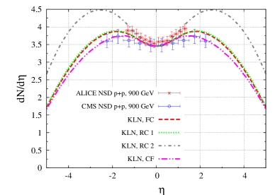
(a)

(b)

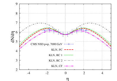
(c)

Figure 1: Pseudorapidity distributions measured in inclusive hadron production in $pp$ collisions for different values of $\sqrt{s}$: (a) $0.9$ TeV, (b) $2.36$ TeV and (c) $7$ TeV. Data are from Refs. Aamodt:2010ft ; Khachatryan:2010xs ; Khachatryan:2010us .

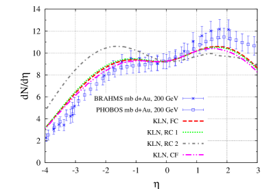
(a)

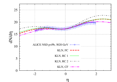
(b)

Figure 2: Pseudorapidity distributions measured in inclusive hadron production in (a) $dAu$ collisions ($\sqrt{s}=0.2$ TeV) and (b) $pPb$ collisions ($\sqrt{s}=5.02$ TeV). Data are from Refs. Arsene:2004cn ; Alver:2010ck ; ALICE:2012xs .

In Fig. 1 we present our results for the pseudorapidity distributions obtained in $pp$ collisions at different center-of-mass energies. The normalization of the different curves, given by the factor $K/\sigma_{s}$ in Eq. (9), has been fixed at each energy in order to reproduce the experimental data at $\eta=0$. The FC and RC1 predictions are very similar, differing of the other results at large $\eta$, whereas the RC2 curve exhibits the steepest rise (and fall) with the pseudorapidity. The CF formula yields a reasonable description of the $pp$ data. We have verified that the necessary change of the normalization between $\sqrt{s}=0.9$ TeV and 7 TeV is smaller than 1.0 % in the case of the CF predictions. On the other hand, for the other predictions, the change was larger than 19%.

In Fig. 2 we present our results for inclusive hadron production in $dAu$ collisions ($\sqrt{s}=0.2$ TeV) and in $pPb$ collisions ($\sqrt{s}=5.02$ TeV). The normalization of the $dAu$ results was chosen so as to describe the data on the deuteron side and in the $\eta=0$ region (within the error bars), simultaneously. On the other hand, in the $pPb$ case, we normalize our predictions in such way that they reproduce the data at $\eta=0$. As observed in our analysis of the $pp$ results, the different models predict a distinct behavior with $\eta$, with the FC and RC1 curves being similar and the RC2 one predicting a steeper dependence. The CF prediction is able to describe the experimental data in a large range of pseudorapidities. The discrepancy appearing at large $\eta$ in $dAu$ collisions can be attributed to the simplified treatment of nuclear geometry used in our calculations. Concerning the change of the normalization $K/\sigma_{s}$ necessary to fit data at different energies, we observe that the smallest change occurs for the CF predictions ($\approx 17$ %), while in the other predictions the change is of order of 40 %. A possible interpretation of this result is that the corrected formula captures important energy dependent higher - order contributions, since the same model of the unintegrated gluon distribution was used in all predictions.

In Fig. 3 we present our predictions for $AuAu$ collisions at $\sqrt{s}=0.2$ TeV and $PbPb$ collisions at $\sqrt{s}=2.76$ TeV. The normalization of the different curves has been fixed in order to reproduce the data at $\eta=0$. The $\eta$ dependence of the different curves is similar, with the CF one providing a reasonable description of the experimental data. In contrast with the $pp$ and $pPb/dAu$ cases, in heavy ion collisions the required change of the normalization, when going from one energy to another, is always large, even in the CF case $[{\cal{O}}(25\%)]$.

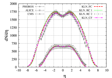
(a)

Figure 3: Pseudorapidity distributions measured in inclusive hadron production in $AuAu$ collisions at $\sqrt{s}=0.2$ TeV (lower curves) and $PbPb$ collisions at $\sqrt{s}=2.76$ TeV (upper curves). Data are from Refs. Back:2001bq ; Back:2002wb ; Abbas:2013bpa ; Chatrchyan:2011pb .

Finally, let us compare the predictions of the different models for the energy dependence of charged hadron multiplicities at $\eta=0$. We will consider $pp$, $pA$ and $AA$ collisions, with the $pA$ and $AA$ predictions being normalized by $\langle N_{\rm part}\rangle$ and $2/\langle N_{\rm part}\rangle$, respectively, where $\langle N_{\rm part}\rangle$ is the average number of participants. We use the values of $\langle N_{\rm part}\rangle$ given in Ref. ALICE:2012xs ; Back:2002uc for minimum bias $pPb$ collisions and the $3\%$ most central $AA$ collisions. As we are interested in the energy dependence of the predictions, we will fix the normalization factors using the experimental data on $dN/d\eta$ in $pp$ collisions at $\sqrt{s}=0.9$ TeV, $dAu$ collisions at $\sqrt{s}=0.2$ TeV and $AuAu$ collisions at $\sqrt{s}=0.13$ TeV. The predictions for higher energies will be parameter free. As can be seen in Fig. 4 the CF curve presents a slower growth with the energy in comparison with the predictions obtained using the original $k_{T}$ - factorization formula. One have that using a simplified model for the unintegrated gluon distribution and a crude treatment of the nuclear geometry, the corrected $k_{T}$ - factorization formula implies a satisfactory description of the $pp$ and $pA$ data. In particular, the CF predictions describe quite well the experimental data from $pp$ collisions at high and low energies, in contrast to the other approaches that using the same inputs fail to reproduce data at $\sqrt{s}<0.9$ TeV. Moreover, the corrected formula provides a prediction for the $pA$ case that is closer to the experimental data. In contrast, the CF predictions underestimate the $AA$ data for high energies, which could indicate that for such systems a more precise treatment of the unintegrated gluon distribution and nuclear geometry is fundamental to describe the data. Surely, such aspects should be investigated in the future.

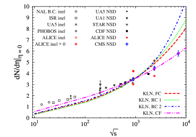
(a)

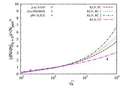
(b)

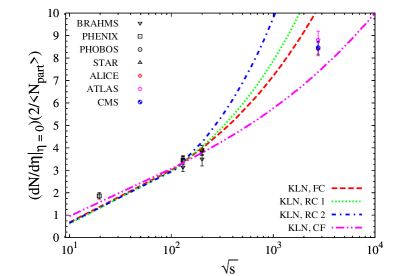
(c)

Figure 4: Energy dependence of charged hadron multiplicities in the central region of rapidity $\eta=0$. (a) $pp$, (b) $pA$ and (c) $AA$ collisions. The $pA$ and $AA$ predictions are normalized by $N_{\rm part}$ and $2/\langle N_{\rm part}\rangle$, respectively. Data are from Refs. Aamodt:2010ft ; Khachatryan:2010xs ; ALICE:2012xs ; Chatrchyan:2011pb ; Back:2002uc ; Whitmore:1973ri ; Thome:1977ky ; Alner:1986xu ; Nouicer:2004ke ; Aamodt:2010pp ; Albajar:1989an ; Abelev:2008ab ; Abe:1989td ; Bearden:2001xw ; Bearden:2001qq ; Adler:2004zn ; Aamodt:2010cz ; ATLAS:2011ag .

IV Conclusions

In the phenomenology of the CGC, the $k_{T}$ - factorization formula, is one of the most important tools. It was originally derived assuming a fixed coupling constant and a collision between a dilute and a dense system. The effect of running coupling corrections on the $k_{T}$ - factorization formula was addressed in Ref. Kovchegov.Horowitz , where a corrected expression was proposed. The study of the implications of these corrections on the observables was analysed, for the first time, in this paper. Considering simplistic assumptions for the nuclear geometry and for the unintegrated gluon distribution, we have estimated the cross section for inclusive hadron production in $pp/pA/AA$ collisions and we have compared our results with the predictions derived from the original formula, from a fixed coupling and also from two different prescriptions for the scale choice in the running coupling constant. We demonstrated that the impact of these corrections on the observables is small, with the predictions of the distinct approaches for the pseudorapidity distributions and charged hadron multiplicities being similar. In particular, we verified that the predictions of the corrected formula yield a satisfactory description of the experimental data. The main difference arises in the energy dependence of the observables, with the corrected formula predicting a weaker energy dependence. Our results motivate more robust calculations considering a realistic unintegrated gluon distribution and a precise treatment of the nuclear geometry. Surely these aspects deserve to be investigated in more detail in the future. However, we believe that the exploratory study performed in this paper shed light on the basic implications of the corrected running coupling $k_{T}$ - factorization formula and that the basic conclusions which emerge from this analysis will remain valid.

- (1) N. Armesto et al., J. Phys. G 35 (2008) 054001; C. A. Salgado et al., J. Phys. G 39, 015010 (2012); J. L. Albacete et al., Int. J. Mod. Phys. E 22, 1330007 (2013)
- (2) Yu. Dokshitzer, Sov. Phys. JETP 46, 1649 (1977); V.N. Gribov and L. N. Lipatov, Sov. Nucl. Phys. 15, 438 (1972); G. Altarelli and G. Parisi, Nucl. Phys. B126, 298 (1977).
- (3) L. N. Lipatov, Sov. J. Nucl. Phys. 23, 338 (1976); E. A. Kuraev, L. N. Lipatov and V. S. Fadin, Sov. Phys. JETP 45, 199 (1977); I. I. Balitsky and L. N. Lipatov, Sov. J. Nucl. Phys. 28, 822 (1978).
- (4) F. Gelis, E. Iancu, J. Jalilian-Marian and R. Venugopalan, Ann. Rev. Nucl. Part. Sci. 60, 463 (2010);E. Iancu and R. Venugopalan, arXiv:hep-ph/0303204; H. Weigert, Prog. Part. Nucl. Phys. 55, 461 (2005); J. Jalilian-Marian and Y. V. Kovchegov, Prog. Part. Nucl. Phys. 56, 104 (2006); J. L. Albacete and C. Marquet, Prog. Part. Nucl. Phys. 76, 1 (2014).
- (5) I. Balitsky, Phys. Rev. D 75, 014001 (2007); I. Balitsky and G. A. Chirilli, Phys. Rev. D 77, 014019 (2008).
- (6) Y. V. Kovchegov and H. Weigert, Nucl. Phys. A 784, 188 (2007); Nucl. Phys. A 789, 260 (2007); Y. V. Kovchegov, J. Kuokkanen, K. Rummukainen and H. Weigert, Nucl. Phys. A 823, 47 (2009).
- (7) E. Iancu, J. D. Madrigal, A. H. Mueller, G. Soyez and D. N. Triantafyllopoulos, Phys. Lett. B 750, 643 (2015)
- (8) T. Lappi and H. Mantysaari, Phys. Rev. D 93, 094004 (2016)
- (9) I. Balitsky, Nucl. Phys. B463, 99 (1996); Y. V. Kovchegov, Phys. Rev. D 60, 034008 (1999); ibid. 61, 074018 (2000).
- (10) A. Dumitru, A. Hayashigaki and J. Jalilian-Marian, Nucl. Phys. A 765, 464 (2006)
- (11) G. A. Chirilli, B. W. Xiao and F. Yuan, Phys. Rev. Lett. 108, 122301 (2012); A. M. Stasto, B. W. Xiao and D. Zaslavsky, Phys. Rev. Lett. 112, 012302 (2014)
- (12) T. Altinoluk, N. Armesto, G. Beuf, A. Kovner and M. Lublinsky, Phys. Rev. D 91, 094016 (2015)
- (13) K. Watanabe, B. W. Xiao, F. Yuan and D. Zaslavsky, Phys. Rev. D 92, 034026 (2015)
- (14) W. A. Horowitz and Y. V. Kovchegov, Nucl. Phys. A 849, 72 (2011).
- (15) L. V. Gribov, E. M. Levin and M. G. Ryskin, Phys. Rept. 100, 1 (1983).
- (16) Y. V. Kovchegov and K. Tuchin, Phys. Rev. D 65, 074026 (2002)
- (17) M. A. Braun, Phys. Lett. B 483, 105 (2000).
- (18) D. Kharzeev and M. Nardi, Phys. Lett. B 507, 121 (2001); D. Kharzeev and E. Levin, Phys. Lett. B 523, 79 (2001); D. Kharzeev, E. Levin and M. Nardi, Phys. Rev. C 71, 054903 (2005); Nucl. Phys. A 747, 609 (2005)
- (19) E. Levin and A. H. Rezaeian, Phys. Rev. D 82, 014022 (2010); Phys. Rev. D 82, 054003 (2010); Phys. Rev. D 83, 114001 (2011).
- (20) J. L. Albacete and A. Dumitru, arXiv:1011.5161 [hep-ph].
- (21) J. L. Albacete, A. Dumitru, H. Fujii and Y. Nara, Nucl. Phys. A 897, 1 (2013).
- (22) A. Dumitru, D. E. Kharzeev, E. M. Levin and Y. Nara, Phys. Rev. C 85, 044920 (2012).
- (23) P. Tribedy and R. Venugopalan, Nucl. Phys. A 850, 136 (2011) Erratum: [Nucl. Phys. A 859, 185 (2011)]; Phys. Lett. B 710, 125 (2012) Erratum: [Phys. Lett. B 718, 1154 (2013)]; B. Schenke, P. Tribedy and R. Venugopalan, Phys. Rev. C 89, 024901 (2014).
- (24) S. J. Brodsky, G. P. Lepage and P. B. Mackenzie, Phys. Rev. D 28, 228 (1983).
- (25) F. Gelis, T. Lappi and R. Venugopalan, Phys. Rev. D 78, 054019 (2008); Phys. Rev. D 78, 054020 (2008); Phys. Rev. D 79, 094017 (2009).
- (26) J. Jalilian-Marian, A. Kovner, L. McLerran and H. Weigert, Phys. Rev. D 55, 5414 (1997); J. Jalilian-Marian, A. Kovner and H. Weigert, Phys. Rev. D 59, 014014 (1999), ibid. 59, 014015 (1999), ibid. 59 034007 (1999); A. Kovner, J. Guilherme Milhano and H. Weigert, Phys. Rev. D 62, 114005 (2000); H. Weigert, Nucl. Phys. A703, 823 (2002); E. Iancu, A. Leonidov and L. McLerran, Nucl.Phys. A692 (2001) 583; E. Ferreiro, E. Iancu, A. Leonidov and L. McLerran, Nucl. Phys. A701, 489 (2002).
- (27) E. Gotsman, M. Kozlov, E. Levin, U. Maor and E. Naftali, Nucl. Phys. A 742, 55 (2004); A. Kormilitzin and E. Levin, Nucl. Phys. A 849, 98 (2011); C. Contreras, E. Levin and I. Potashnikova, Nucl. Phys. A 948, 1 (2016).
- (28) K. J. Golec-Biernat and A. M. Stasto, Nucl. Phys. B 668, 345 (2003).
- (29) J. Berger and A. Stasto, Phys. Rev. D 83, 034015 (2011); Phys. Rev. D 84, 094022 (2011); JHEP 1301, 001 (2013)
- (30) K. J. Golec-Biernat and M. Wusthoff, Phys. Rev. D 59, 014017 (1998).
- (31) S. J. Brodsky and G. R. Farrar, Phys. Rev. Lett. 31, 1153 (1973).
- (32) V. A. Matveev, R. M. Muradian and A. N. Tavkhelidze, Lett. Nuovo Cim. 7, 719 (1973).
- (33) K. Aamodt et al. [ALICE Collaboration], Eur. Phys. J. C 68, 89 (2010).
- (34) V. Khachatryan et al. [CMS Collaboration], JHEP 1002, 041 (2010).
- (35) V. Khachatryan et al. [CMS Collaboration], Phys. Rev. Lett. 105, 022002 (2010).
- (36) I. Arsene et al. [BRAHMS Collaboration], Phys. Rev. Lett. 94, 032301 (2005).
- (37) B. Alver et al. [PHOBOS Collaboration], Phys. Rev. C 83, 024913 (2011).
- (38) B. Abelev et al. [ALICE Collaboration], Phys. Rev. Lett. 110, no. 3, 032301 (2013).
- (39) B. B. Back et al. [PHOBOS Collaboration], Phys. Rev. Lett. 87, 102303 (2001).
- (40) B. B. Back et al., Phys. Rev. Lett. 91, 052303 (2003).
- (41) E. Abbas et al. [ALICE Collaboration], Phys. Lett. B 726, 610 (2013).
- (42) S. Chatrchyan et al. [CMS Collaboration], JHEP 1108, 141 (2011).
- (43) B. B. Back et al. [PHOBOS Collaboration], Phys. Rev. C 65, 061901 (2002).
- (44) J. Whitmore, Phys. Rept. 10, 273 (1974).
- (45) W. Thome et al. [Aachen-CERN-Heidelberg-Munich Collaboration], Nucl. Phys. B 129, 365 (1977).
- (46) G. J. Alner et al. [UA5 Collaboration], Z. Phys. C 33, 1 (1986).
- (47) R. Nouicer et al. [PHOBOS Collaboration], J. Phys. G 30, S1133 (2004).
- (48) K. Aamodt et al. [ALICE Collaboration], Eur. Phys. J. C 68, 345 (2010) doi:10.1140/epjc/s10052-010-1350-2 [arXiv:1004.3514 [hep-ex]].
- (49) C. Albajar et al. [UA1 Collaboration], Nucl. Phys. B 335, 261 (1990).
- (50) B. I. Abelev et al. [STAR Collaboration], Phys. Rev. C 79, 034909 (2009).
- (51) F. Abe et al. [CDF Collaboration], Phys. Rev. D 41, 2330 (1990).
- (52) I. G. Bearden et al. [BRAHMS Collaboration], Phys. Lett. B 523, 227 (2001).
- (53) I. G. Bearden et al. [BRAHMS Collaboration], Phys. Rev. Lett. 88, 202301 (2002).
- (54) S. S. Adler et al. [PHENIX Collaboration], Phys. Rev. C 71, 034908 (2005) Erratum: [Phys. Rev. C 71, 049901 (2005)].
- (55) K. Aamodt et al. [ALICE Collaboration], Phys. Rev. Lett. 106, 032301 (2011).
- (56) G. Aad et al. [ATLAS Collaboration], Phys. Lett. B 710, 363 (2012).